
Reducing Simulation Performance Gap in Hemp-Lime Buildings Using Fourier Filtering † †

Zero Carbon Lab, Birmingham City University, Birmingham B5 5JU, UK
†
This paper is an extended version of our conference work “A method for eliminating simulation performance gap in buildings built form natural fibrous materials”. In Proceedings of the 2014 Building Simulation and Optimization Conference, 23–24 June 2014, London, UK.
Sustainability 2016, 8(9), 864; https://doi.org/10.3390/su8090864
Submission received: 30 June 2016
/
Revised: 15 August 2016
/
Accepted: 19 August 2016
/
Published: 29 August 2016
(This article belongs to the Special Issue Advances in Post Occupancy Evaluation)
Abstract
:Mainstream dynamic simulation tools used by designers do not have a built-in capability to accurately simulate the effect of hemp-lime on building temperature and relative humidity. Due to the specific structure of hemp-lime, heat travels via a maze of solid branches whilst the capillary tubes absorb and release moisture. The resultant heat and moisture transfer cannot be fully represented in mainstream simulation tools, causing a significant performance gap between the simulation and the actual performance. The author has developed an analysis method, based on a numerical procedure for digital signal filtering using Fourier series. The paper develops and experimentally validates transfer functions that enhance simulation results and enable accurate representation of behaviour of buildings built from hemp-lime material using the results of a post-occupancy research project. As a performance gap between design simulation and actual buildings occurs in relation to all buildings, this method has a wider scope of application in reducing the performance gap.
1. Introduction
Dynamic simulation is the only building design tool that enables reasonably accurate relative comparison between different design options. Dynamic simulation is however far less accurate in predicting the absolute performance of the chosen design [1]. This inaccuracy is caused by differences between the actual building and the representation of its properties in the simulation model. Specifically, the theoretical values of heat transfer properties of building materials may not correspond to the actual properties, due to different chemical composition and moisture content; behaviour of building users in the actual building may be oversimplified in the simulation model; and the build quality of the actual building, as it often happens, may be worse than the theoretical representation of the building in the simulation model. These differences between the actual and the simulated building are the main causes of the performance gap, however, in the case of hemp-lime bio-composite material, this is exacerbated by the absence of its accurate theoretical description in the simulation model.
The existence of the performance gap caused by inaccurate simulation leads to practical problems: over-specification of the heating or cooling plant, increased capital cost, prolonged part-load operation of the plant, increased running costs, increased energy consumption, and increased carbon dioxide emissions.
In addition to the general causes of the performance gap, mainstream simulation tools used by designers, such as DesignBuilder by DesignBuilder Software Ltd. (Stroud, UK), IES Virtual Environment by Integrated Environmental Solutions, TAS by Environmental Design Solutions Ltd., TRNSYS—A Transient System Simulation Program from the Solar Energy Laboratory of the University of Wisconsin, and others, do not have a built-in capability to accurately represent the effect of hemp-lime material on building temperature and relative humidity. In the most simplified description, hemp-lime material consists of shredded hemp bonded with lime. On a macroscopic level, the resultant structure comprises of a maze of interconnected solid pieces, surrounded by capillary tubes created as result of the bonding of the pieces into porous blocks. On a microscopic level, hemp has its own capillary mechanisms for absorbing and releasing moisture. Thus, the resultant behaviour of the building material is far more complicated than that can be described in a simulation model: Heat transfer takes place through the maze of interconnected solid pieces, and moisture is absorbed and released by the macroscopic and microscopic capillary tubes. The overall behaviour of the material includes sensible and latent heat transfer, as well as moisture balancing with the environment.
To define a material in a simulation model, such as IES, the user needs to define its thermal conductivity, density and specific heat capacity. These three properties enable the simulation model to calculate thermal diffusivity of the material [2], which is subsequently used in the dynamic simulation. Moisture transfer property is specified through vapor resistivity. However, by defining the properties of the material in this way, the effect of multiple conductivity through individual pieces of hemp, the sensible and the latent heat transfer, and the moisture transfer and balance through macro and micro mechanisms in hemp-lime material do not appear to be adequately defined in the simulation model. Although recent research results contribute to an increased understanding of the hygrothermal properties of hemp-based materials [3], this has not yet been reflected in the mainstream simulation tools. Whilst elements for specifying various properties of hemp-lime material, such as sorption isotherms, water-vapour diffusivity, heat and moisture transfer exist in a Combined Heat and Moisture Transfer (HAMT) Model in EnergyPlus [4], and have been used for experimental research in this field [5], it is not yet possible to find a ready made hemp-based material within mainstream simulation tools used by designers.
The resultant heat and moisture transfer mechanisms are, therefore, far more complicated than currently represented in the mainstream dynamic simulation models, thus resulting in considerable performance gap between dynamic simulation design analysis and buildings constructed from this material.
For this reason, it was not deemed necessary to investigate the problem with other building performance simulation tools that can handle latent heat transfer, as the manufacturers of hemp-lime material only provide sensible heat transfer properties, and, therefore, no benefit would be gained by using a simulation tool that can handle both sensible and latent heat transfer.
Dynamic simulation models can be tuned to accurately represent the performance of an existing building through a process called calibration. Monitored weather and performance data are used to adjust the simulation model parameters so as to minimise the error between the simulated and the actual performance. As the concept of calibration requires a comparison between a parameter value provided by an “instrument” (in our case a simulation model) and the measured value of that parameter, calibration is applicable only to investigating the behaviour of existing buildings which can be monitored.
The attractiveness of Fourier filtering methods is that they can offer transferable features between simulation models of existing and non-existing buildings by establishing an essence of building thermal behaviour in the form of a response function, referred to as a Fourier filter in this paper. Other types of methods, such as neural networks, were also considered [6], but did not offer transferable features between simulation models, due to limitations in simulating time delayed relationships between inputs and outputs at scales that exist in building materials.
The development of a Fourier filter based upon the results of IES Virtual Environment simulation was inspired by methods from another field, namely digital signal processing of sound waves. Fourier filtering methods are routinely used in that field for noise filtering [7], but this work demonstrates that these methods can also be used for morphing of time series from building simulation into more realistic behaviour.
2. Materials and Methods
In the 19th Century, the French mathematician Fourier demonstrated that every periodic function could be represented with a combination of a series of sine and cosine waves with varying amplitudes and frequencies. The expression for a discrete Fourier transform (DFT) is as follows:
Due to computational limitations of the DFT associated with higher number of harmonics [8,9], the method reported in this paper will use the FFT—the Fast Fourier Transform [10], which has no limitations on the number of harmonics.
On this basis, a response function between monitored and simulated performance of an experimental building will be created as a ratio (de-convolution) between corresponding Fourier transforms. The response function will then be applied as a filter to a digital signal obtained from a simulation of another building. Assuming that the experimental building and the other building are of similar types, both built from hemp-lime material of similar properties, the convolution of the signal from the other building and the response function will be equivalent to the results of instrumental monitoring of that other building.
Why the use and creation of filters and the Fourier filtering Method? Fourier transform is suitable for the representation of periodic functions, with exceptional accuracy. As previously reported, the root mean squared error between an original data set of hourly annual room temperatures and its Fourier transform was found to be equal to 0.0005 °C [8]. This means that a data set of hourly room temperatures for the entire year can be represented with a single function with a very high accuracy. Establishing a relationship between two such data sets, for instance between simulated and monitored, becomes easily possible through establishing a relationship between the corresponding Fourier transforms.
The work presented in the paper will use two existing monitored buildings: measurements were performed in an experimental building named Hempod and in an existing terraced house, and the latter will represent a building on a “drawing board” (a future building) and will be used to validate the method.
The summary of design parameters of the existing terraced house is as follows: ground floor 0.15 W/(m2K); external walls 0.19 W/(m2K); roof 0.13 W/(m2K); windows 1.2 W/(m2K). The total design heat loss coefficient derived from these figures was 44.51 W/K. The design air permeability was 2.1 m3/h/m2. These design figures were considerably different from those obtained from co-heating tests and air tightness tests: 69.28 W/K for heat loss coefficient, and 3.61 m3/h/m2 for measured air permeability. Details of the measurements and the reasons for discrepancies between design and measured values are discussed in Reference [11].
The method can therefore be summarised in the following steps, customising the approach in Reference [8] for the application to hemp-lime material:
- (1)
- create a dynamic simulation model of an existing building built from hemp-lime material, which is also being monitored;
- (2)
- represent the time series of the monitored and simulated parameters, such as temperature or relative humidity, as separate Fourier transforms;
- (3)
- assume that the monitored time series is the result of a certain response function acting on the simulated time series (in other words that the monitored time series is the result of convolution between the simulated time series and the response function) and obtain the response function through de-convolution of the two corresponding Fourier transforms; this response function is named a “Fourier filter”;
- (4)
- create a dynamic simulation model of a future building built from hemp-lime material and obtain time series of its performance parameters, such as temperature or relative humidity;
- (5)
- represent the time series obtained through dynamic simulation as Fourier transforms;
- (6)
- create a convolution between the Fourier transforms from the previous step and the Fourier filter;
- (7)
- the result is a representation of a time series of a monitored parameter for the future building built from hemp-lime material (a building that is at the design stage and therefore non-existing).
This method is now specified using mathematical formalism and the definitions in the Nomenclature section of this paper. The objective is to obtain:
mi,f, 1 ≤ i ≤ K
This is done firstly by creating the Fourier filter as a de-convolution of the series Mi,e and Si,e:
Rj = Mi,e/Si,e
Having obtained the Fourier filter, the Fourier transform of the simulated time series of the future building si,f is obtained as Si,f. Subsequently, multiplication of the two Fourier transforms Si,f and Rj gives:
and the inverse Fourier transform, as explained by Press et al. [10], achieves the objective from Equation (2):
Si,f Rj = Mi,f
Mi,f ⇒ mi,f, 1 ≤ i ≤ K
2.1. Practical Application of the Method
A practical application of the method outlined in the previous section requires special handling of the filter and the signal, which will be explained in this section.
2.1.1. Creating the Filter
Time series used for the creation of filter were chosen from a period in the monitoring data in which the experimental building, named Hempod, was not exposed to any sudden external influences, such as a change from overcast to sunny weather. Data from monitoring of the Hempod, and from IES simulation of the same building were used, and the input weather data file in IES was amended to include external parameters from the monitoring.
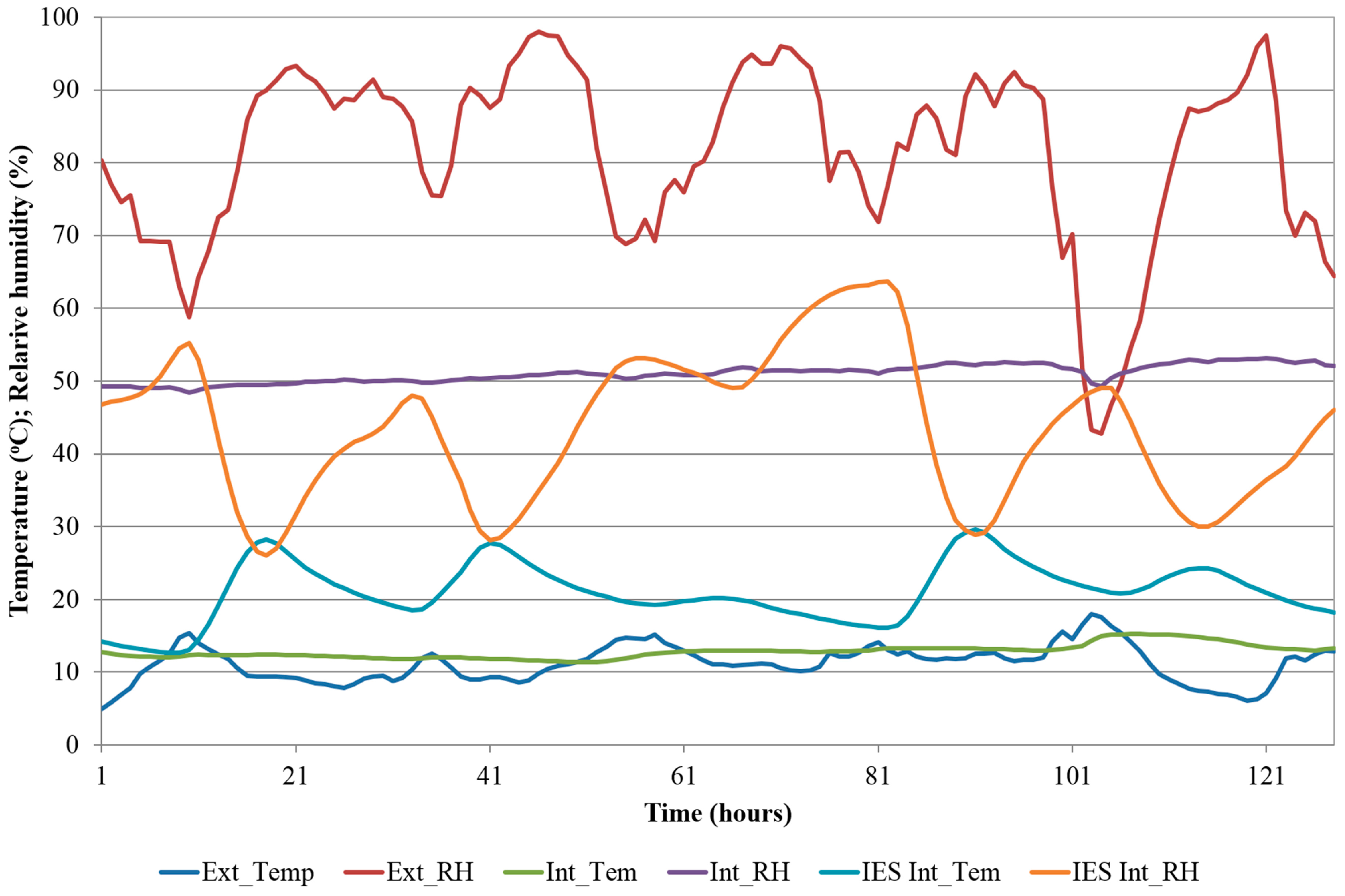
The FFT algorithm can only deal with the number of points equal to the power of two [10], so that N = 2m, where m = 1, 2, 3, …, etc. Therefore the length of the time series used for creating the filter, restricted by the number of available points, was chosen to be 27 = 128 (Figure 1).
This now enables the creation of Fourier filters for temperature and relative humidity, as de-convolutions (ratios) of Fourier transforms of the individual time series, as per Equation (3). Thus, a de-convolution between Fourier transforms of measured and simulated relative humidity will enable the application of the filter on the relative humidity simulation results of another (future) building. A de-convolution between Fourier transforms of measured and simulated temperatures will enable the application of the filter on the internal temperature simulation results of another (future) building, as per Equations (4) and (5).
The “future building” in this context is simply a building “on a drawing board”, a building that is being designed and therefore it does not physically exist and its actual performance cannot be established through instrumental monitoring.
2.1.2. Applying the Filter
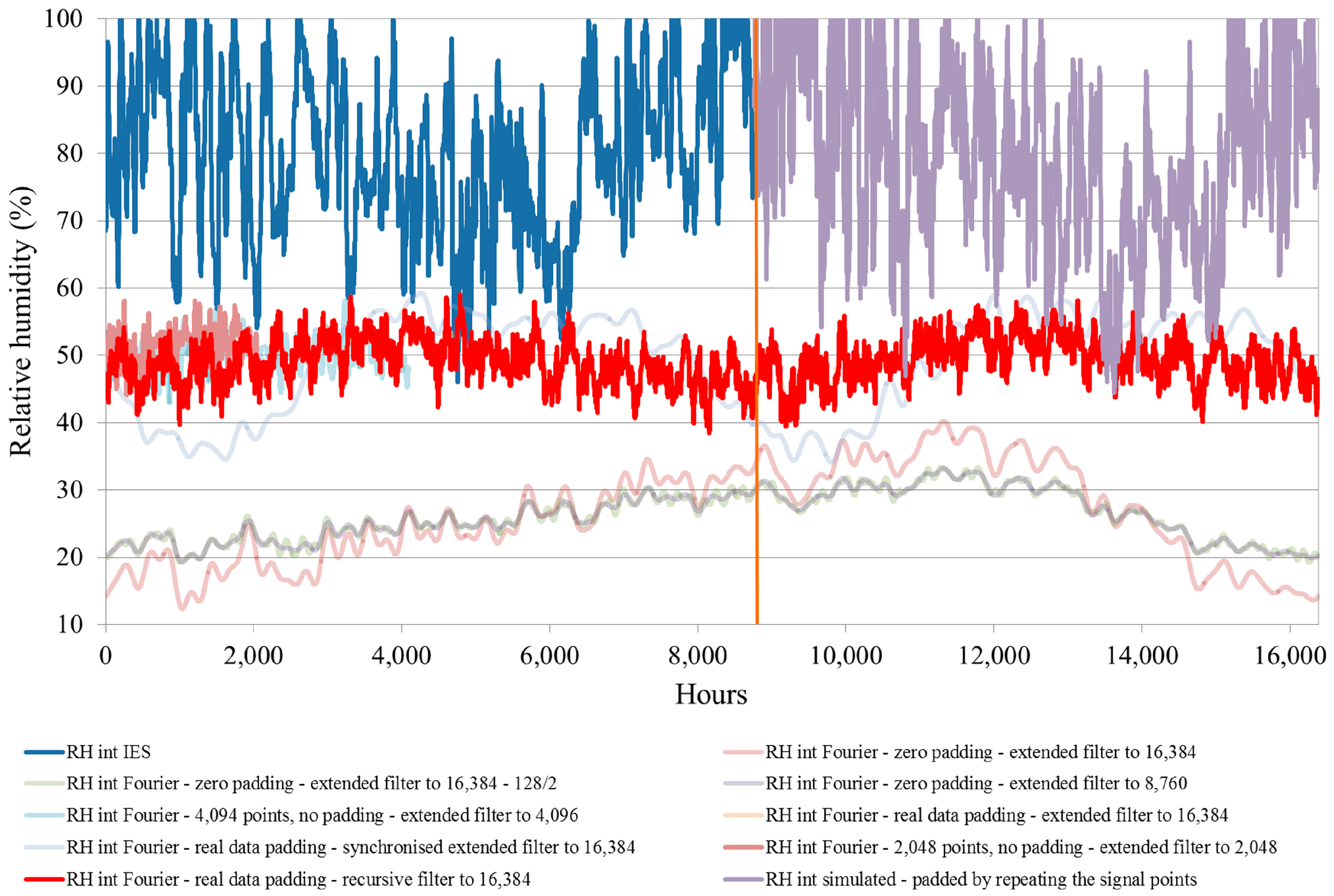
Annual simulations carried out with an hourly time step produce 8760 data points per parameter. Bearing in mind the power of two restriction for the FFT points, 8760 lies between 213 = 8192, and 214 = 16,384. The former number of points does not cover the full annual number of hours, and the latter exceeds them. We, therefore, need to use the latter number to cover the entire annual simulation of a building with an hourly time step. The remaining data points between 8761 and 16,384 need to be filled with values that do not distort the result. In order to identify the extent of potential result distortion, experiments with different data padding approaches were carried out (Figure 2).
Press et al. [10] suggest zero-padding of the points beyond those that exist in the data set. However, this approach resulted in a distortion of the result (Figure 2), and much better result was achieved by replicating the remaining data points between 8761 and 16,384 with the actual input signal data from the start, so that point 1 was copied into point 8761, point 2 into 8762, and so on until all points to 16,384 were filled.
There were similar issues with the filter, which was 128 points long and required padding to make it match 16,384 signal points. Press et al. [10] suggest splitting the filter into halves, placing the first half at the start of the time series, the second half at the end, and zero-padding between the two halves. A filter split in this way is referred to as the “extended filter” in Figure 2. A synchronised extended filter in Figure 2 is a split-filter in which the peaks of frequency in the filter data are aligned manually with the corresponding peaks in signal data. This and various other zero-padding approaches were investigated until it was found that a recursive filter, which was repeated as many times as needed in order to match the number of signal points, achieved the best result (Figure 2). As similar issues occur with temperature filtering, the choice of relative humidity as reference was of no particular significance.
3. Results
The method developed in the previous section will now be applied to an existing terraced house built from hemp-lime material. The application of the Fourier filtering method will help to determine the accuracy of this method and its implications on design of buildings that are on a “drawing board”.
The house in question was under continuous monitoring of temperature and relative humidity over a period of two years, whilst air tightness tests (Figure 3) and a co-heating test (Figure 4) were also carried out during several weeks within that period.
As explained in Reference [12], the house was unoccupied during the monitoring period, and had only a minimum heat input during the winter months, except in the first 10 days of January 2012 when a co-heating test was carried out. Thermal imaging after the co-heating test, combined with air tightness testing, revealed good consistency of the masonry construction with no thermal leaks through hemp-lime material (Figure 5a), whilst the majority of the heat losses occurred through conventional components (Figure 5b).
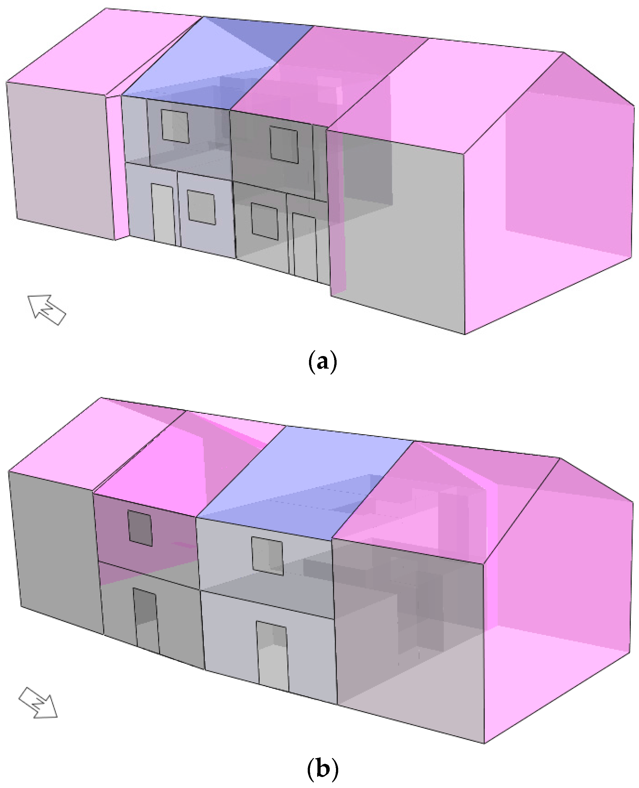
An IES simulation model of the terraced house was subsequently developed, based on drawings and technical specifications, and using the results of air tightness tests (Figure 6).
Before the simulation of the terraced house was carried out, the weather data file was partially synthesised using an EnergyPlus Weather (EPW) file for the specific location, and consulting the corresponding technical documentation [13].
Relevant parameters were replaced either with values obtained from monitoring (dry bulb temperature, relative humidity, global horizontal radiation), or with values derived from monitored data (dew point temperature, as per Reference [14], and direct normal radiation and diffuse horizontal radiation, as per Reference [15]).
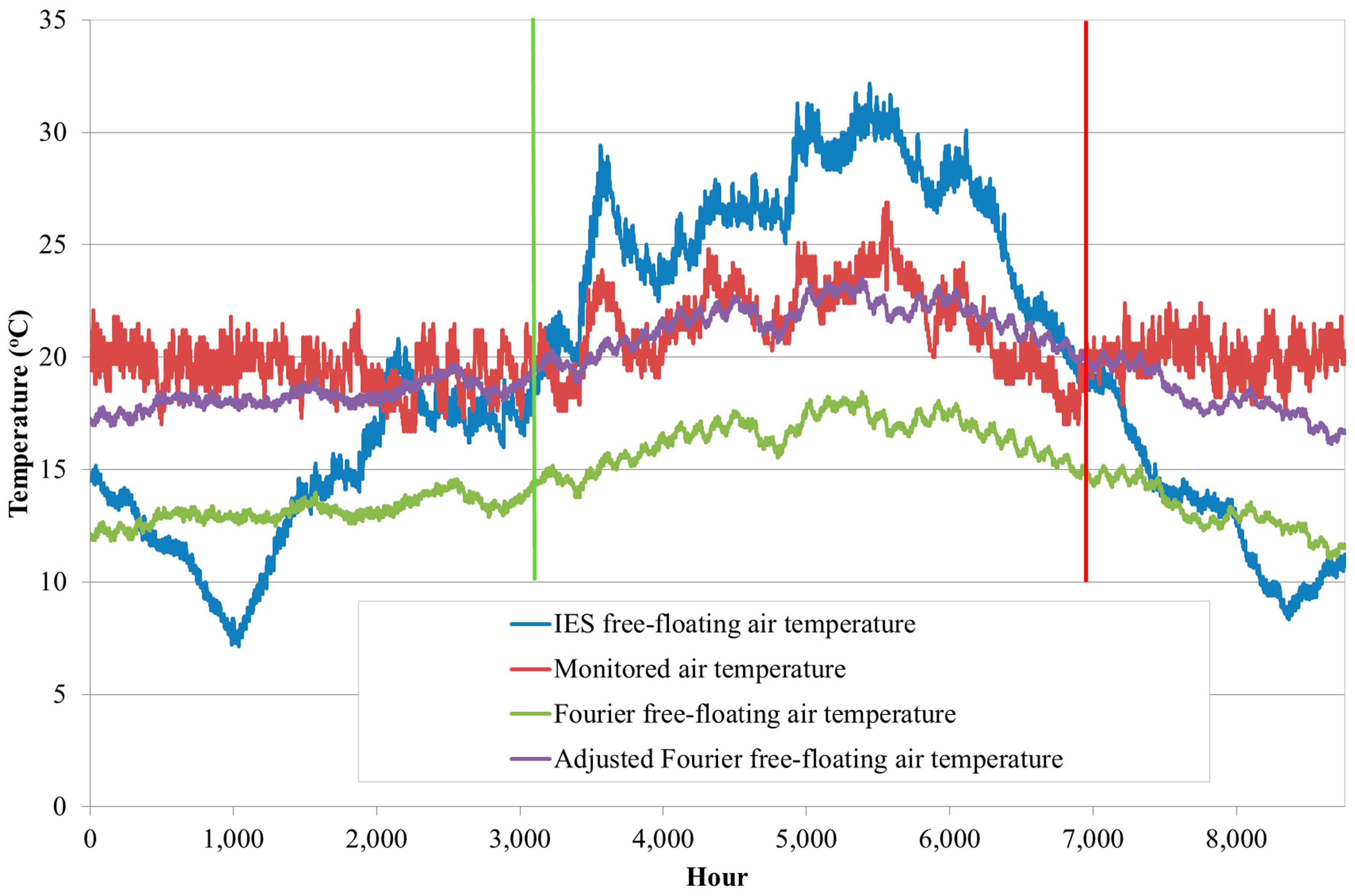
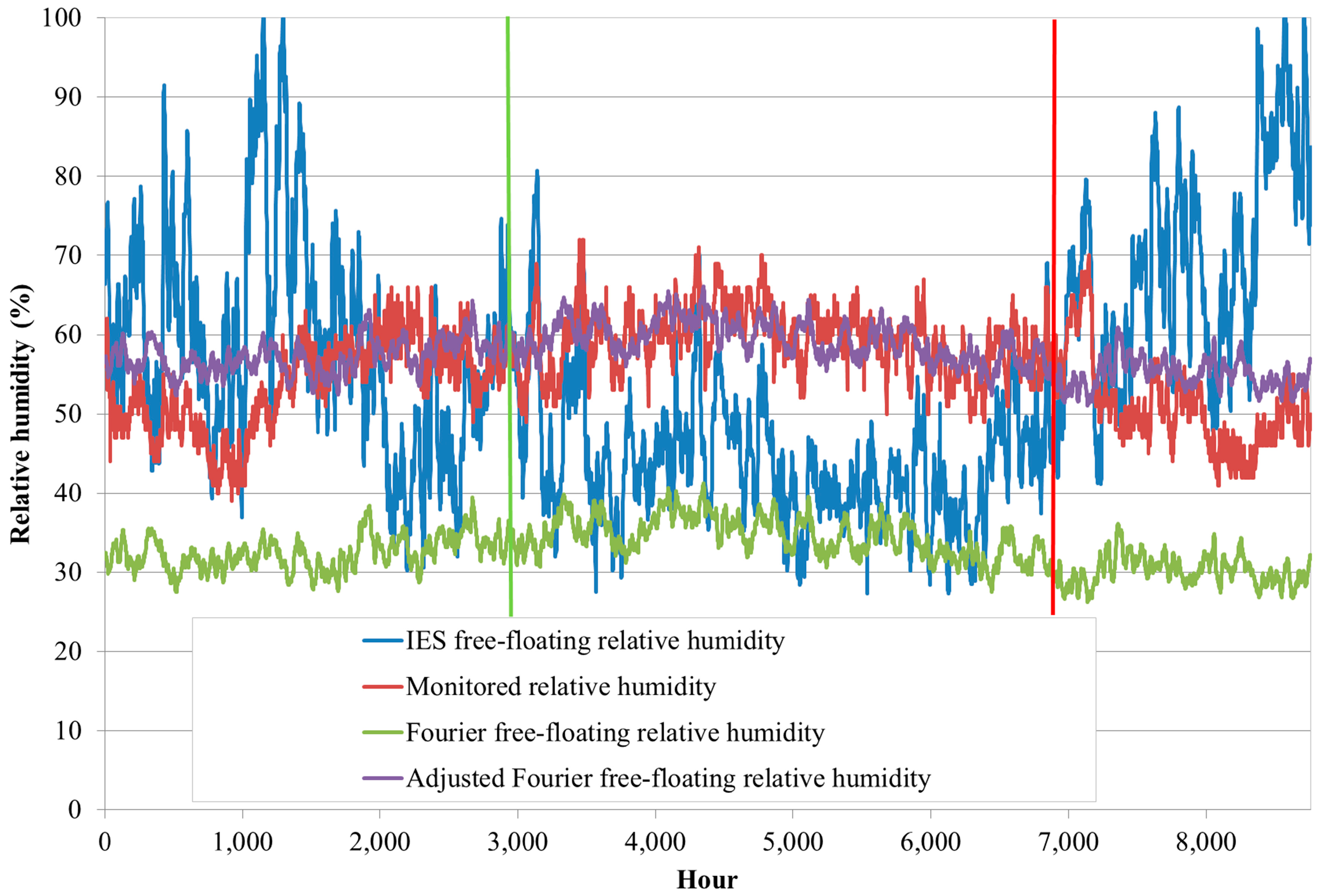
The Fourier filter was then applied to the outputs of IES simulation and the results are shown in Figure 7 and Figure 8. During the period between the vertical green and red lines in Figure 7 and Figure 8, corresponding to the period between days 136 and 287, there was no heat input into the house. As the experimental building from which the Fourier filter was derived had been unheated and therefore in a free-floating mode, the unheated period in the terraced house, shown between the green and red vertical lines in Figure 7 and Figure 8, was chosen for this analysis.
Figure 7 shows the comparison between IES temperature, Fourier filtered temperature, and monitored air temperature of the living room of the terraced house. The Fourier filtered temperature profile was adjusted so that its average during the unheated period was aligned with the average of the monitored temperature during the same period. In practice, this alignment would occur as result of heating prior to the unheated period.
In order to assess how close the results of analysis were to the monitored data, a root mean squared error (RMSE) was used, as defined in Equation (6):
The analysis of temperatures in Figure 7 shows that the RMSE between the IES simulation and the monitored temperature during the unheated period was 4.89 °C, and the RMSE between the adjusted Fourier temperature and monitored temperature was 1.48 °C. The relative magnitudes of these errors are a quantitative representation of the discrepancies shown in Figure 7: The IES simulation appears to be very inaccurate, with a considerable performance gap, and the adjusted Fourier temperature appears to have a considerably smaller performance gap.
The analysis of relative humidity is shown in Figure 8. Similarly to the alignment of temperature curves in the previous figure, the Fourier transform of the relative humidity was aligned with the monitored relative humidity by adjusting its average fluctuation to be equal to the average fluctuation of the monitored relative humidity during the unheated period. In practice this would be achieved by initial humidity regulation.
As can be seen from this figure, whilst the IES-simulated relative humidity shows considerable fluctuations and the RMSE of 16.89%, the adjusted Fourier filtered relative humidity follows the monitored relative humidity much closer, with the RMSE of 4.12%.
This analysis, therefore, demonstrates that a Fourier filter obtained from an experimental building and applied on the results of simulation of another building has considerably reduced the simulation performance gap of that other building, both in terms of air temperature and relative humidity. However, as the RMSE between the adjusted Fourier curves and the monitored curves is non-zero, the question arises as to what are the design implications of this method? This will be analysed in the next section.
4. Discussion
4.1. Design Implications
The attenuated fluctuations of temperature and relative humidity resulting from the application of the Fourier filter will inevitably result in choosing a smaller plant size with a consequence of lower capital cost and lower energy consumption, in comparison with designs made on the basis of dynamic simulation alone. But how would this reduction be estimated?
It is reasonable to assume that the reduction of the energy consumption will be proportional to the ratio between the temperature fluctuations before and after the filtering, and taking into account the RMSE, which would give the upper and lower boundary of the reduction range. Evidence from our design projects suggests that the same could be true of the installed plant capacity. This can be expressed using the positive differences between the desired value (such as the set temperature) and the fluctuating values in the case of heating, and the negative differences in the case of cooling, as shown in Equations (7) and (8).
As the internal air temperature was monitored and therefore known, the set temperature in this analysis was replaced with the actual monitored temperature. Substituting the corresponding values in Equations (7) and (8), the following results were obtained:
This means that, as result of the application of this method, the mechanical plant can be between 50% and 80% smaller in the case of heating, and between 69% and 93% smaller in the case of cooling. There will be similar reduction in energy consumption, carbon emissions and running costs. Applying the same method of calculation to relative humidity, the reduction of a humidification plant size is estimated to be 0.83 ± 0.09, and the reduction of a dehumidification plant size is estimated to be 0.48 ± 0.19. This means that the humidification plant will be between 74% and 92% smaller, and the dehumidification plant will be between 29% and 67% smaller. There will be equivalent savings on the running costs of humidification and dehumidification.
4.2. Results Overview
The method presented in this paper can be regarded as an extrapolation of monitored data from an existing building applied to another building that has not yet been built.
Although extrapolation can often lead to unexpected errors, the rigour of the method presented here gives a reasonable expectation of its accuracy and a potential to reduce the performance gap between dynamic simulation and actual building performance in buildings built from hemp-lime material.
There are no critical inputs required for the simulation model in order to perform Fourier analysis, except that the simulated building needs to be based on the same materials as the source building used for generating the filter, and the simulation needs to be carried out in a free floating mode, with no heating or cooling input.
Although the scale of estimated savings is in a relatively wide range, between 50% and 80% in the case of heating, and between 69% and 93% in the case of cooling, the bottom line is that there is at least 50% of savings on the heating plant size and running costs, and at least 69% savings on the cooling plant size and running costs.
The savings will inevitably depend on the heating and cooling set temperatures, and on the desired humidity setting in the BEMS, and therefore the above reported savings would change with these different settings. However, the RMSE would remain the same, and therefore designers can use it in Equations (7) and (8) and estimate the savings for the particular BEMS settings. For instance, for heating set temperature of 19 °C, Equation (7) gives the saving of heating energy Sh = 0.83 ± 0.12, therefore between 71% and 95%. For cooling set temperature of 24 °C, the saving of cooling energy calculated on the basis of Equation (8) is Sc = 1, therefore 100%.
4.3. Application and Constraints
To recap, why the use and creation of filters and the Fourier filtering Method? As explained in the Introduction, the Fourier transform is suitable for representation of periodic functions, and buildings are driven by periodic functions of external air temperature, solar radiation, and internal occupancy patterns. Fourier transforms are exceptionally accurate representations of data, so that the root mean squared error between the original data set of hourly annual room temperatures and its Fourier transform was found to be 0.0005 °C [8]. Once a time series of hourly simulation of room temperatures is encapsulated in a Fourier transform, it is easy to establish its relationship with a Fourier transform of the measured room temperature, and the relationship between the two, named a Fourier filter, is subsequently used for minimising the simulation performance gap.
What conditions the experimental building needs to meet in order to generate the Fourier filter and to what other kinds of buildings this can be applied? Although the analysis in this paper was based on a relationship between an experimental building and a two bedroom terraced house, it is believed that this approach is scalable to larger buildings, as both were analysed in free floating mode without any heating or cooling input in the simulation model, and the two bedroom house was much larger than the experimental building. This will need to be confirmed by further research. Different geometries, orientations, percentage of glazing and different climates need to be investigated as part of a future development of this method. The future work will also investigate the dynamic variation of the filtered temperature and relative humidity over a wider range of conditions and will aim to bring them closer to the monitored values.
What is the effect of occupancy on the performance gap? The analysis building temperatures that was used to derive the Fourier filter was based on unoccupied buildings, running in a free-floating mode. This analysis therefore deals with the passive regulation of the hemp-lime material, regardless of the influence of any additional forcing functions, including occupancy patterns. These additional forcing functions will need to be investigated through future research, however it is believed that their influence will be subjected to the same attenuation on the building temperatures as the influence of external driving functions.
Could it be that the way in which the performance gap is calculated is wrong? Or could it be that the monitoring method was incorrect and that the simulation was close to reality? On the one hand, the monitoring data comes from a calibrated system, and, therefore, it is unlikely to be inaccurate. On the other hand, the existence of the performance gap has been established through a body of independent research, and methods for its elimination are linked to post occupancy evaluation [16]. The work reported in this paper goes beyond the conventional post occupancy evaluation, by transferring POE results from an existing to a non-existing building.
4.4. Notes on Signal and Filter Padding
As shown earlier in the paper, zero-padding of the signal and the filter leads to a distorted filtered signal. Different numbers of zero-padded points will lead to different average values of the filtered signal, and thus cannot be considered as a realistic result. The approach discussed in this paper shows that replacing the zero-padding of the signal with padding using actual signal points leads to consistent average values of the filtered signal, and therefore to a more realistic result.
The zero-padding of an extended filter leads to unrealistic smoothing of the fluctuations of the filtered signal. Longer signal and filter pairs with larger number of zero-padded filter points lead to greater smoothing of the filtered signal. Thus the result of filtering which involves zero-padding is affected by the length of the data set and therefore it cannot be considered to represent the behaviour of the modelled building. Replacing the zero-padding in the filter with repeating the filter points to match the number of signal points, results in more realistic fluctuations of the filtered signal that is unaffected by the length of the data set, and it is therefore a much better candidate for accurate representation of the behaviour of the modelled building.
4.5. Notes on the Length of the Time Series Used for Creating the Filter
The length of the time series used for creating the filter was 128 h, therefore just over 5 days. Would this be enough for accurate representation of the building dynamics and would Fourier filters be the same throughout different seasons? Experimental measurement of physical parameters of buildings [9] resulted in a time constant of 44.5 h in a three-bedroom house characterised by high thermal mass construction. This result was consistent regardless of the range of heat inputs the building was exposed to during the experiment. The time constant is defined as the time required for a system response to reach just over 63% of its final value after being exposed to an external input.
As the Fourier filter captures the building dynamics, it can be argued that 128 h, being much longer than the time constant, is more than sufficient to create an accurate representation of the building thermal response, assuming that the building is exposed to a range of inputs representative of those occurring throughout the year. As evidence from Reference [9] shows that the same time constant was calculated for different magnitudes of heat inputs, the conditions considered to be representative are just the changes of weather conditions and not the magnitude of such changes, i.e., the variability changes and not the magnitude of changes. On this basis, 128 h would appear to be sufficient to capture the building dynamics regardless of the time of the year or a part of the heating season.
4.6. The Motivation for and the History of the Development of this Method
The method presented in this paper was developed in response to requirements from industry. Initially, I was approached by a client who wanted to develop a winery building using hemp-lime material and knew of another building where considerable smoothing of internal temperature fluctuations and moisture balancing was achieved by a hemp-lime biocomposite.
In order to respond to this request, I revisited some of the work on Fourier series that I did during my PhD [9], which was based on manual spreadsheet calculations of discrete Fourier transform (DFT). This was the basis for the development of the first filter based on Equation (3). As the DFT calculated in this way was time consuming even for three harmonics, I started using the FFT available in the data analysis section of Excel spreadsheet, but this had some other limitations. For instance, the maximum number of data points that could be used to apply the FFT in Excel was 4096. This meant that the entire simulation year of 8760 points could not be analysed in one go. As the FFT works with 2m points, and as 211 = 2048 was a too short time series, 212 = 4096 had to be used. The full simulation year of 8760 points had to be therefore split into three parts of 4096 points. Additionally, as the full length of 3 × 4096 = 12,288 was considerably longer than the full simulation year, there had to be an overlap between the three parts. This itself required manual handling of data in order to split the full simulation year and position the overleaping points. The additional complication was the long execution time, so that the entire process of preparation of data, the running of the FFT algorithm, and the aggregation of the results from the three parts into a single data set of 8760 points, altogether took 3–4 h for each simulation case.
Having seen the value in these outputs, which suggested much more stable internal conditions than anticipated on the basis of simulations, the client started coming back with design variations, and each of these variations was taking several hours to analyse. This approach could not be sustained much longer if the method was to be applied in many more cases.
This is when I decided to develop a bespoke FFT convolution and de-convolution software program in Java. The outcome paid off in terms of time savings. Firstly, there was no longer the need to break the full simulation year into three parts, but instead 214 = 16,384 points were used for the FFT, and the positions from 8761 onwards in the time series were padded as explained in Section 2.1.2. Secondly, the speed of FFT execution in the Java code was 545 milliseconds on a 2.6 GHz Intel Core i7 laptop, therefore less than one second, which represented a considerable time saving in comparison with several hours of the semi-manual work. This improved approach enabled the application of the method to a number of building design projects, as explained in the next section.
4.7. Types and Sizes of Buildings Designed Using this Method
The improvements in the method explained in the previous section enabled the design application in the following building types and sizes (Table 1).
Some of these buildings have been built and have been in operation for several years; some are in the design stage; and some were not built from hemp-lime material after all, as decided by respective clients for variety of reasons. In the buildings that have been built, the application of this method has typically cut the capital cost of M&E services by two thirds.
5. Conclusions
A discrepancy between design simulations and performance of an actual completed building occurs on a regular basis. This is commonly referred to as a “performance gap” and it is a major reason for building underperformance. The performance gap occurs in buildings made from well-known materials, and even more so in buildings made from new materials, such as hemp-lime material, which do not have an accurate and complete description in the mainstream simulation software programs.
A method for reducing the performance gap of buildings made from hemp-lime material has been developed using principles for digital signal processing based on Fourier series. A digital filter that captures the relationship between Fourier transforms of monitored and simulated values of a relevant result in an existing experimental building was first developed. The filter was then applied to simulation outputs of a two-bedroom terraced house, morphing the simulation results into values that are closer to the actual monitored results than those obtained from the simulation. This was validated experimentally.
The consequent reduction of heating plant size and of the corresponding energy consumption and carbon emissions was estimated to be in the range between 50% and 80% in the case of heating, and between 69% and 93% in the case of cooling. Similarly, it was found that a humidification plant would be between 74% and 92% smaller, and a dehumidification plant would be between 29% and 67% smaller, with equivalent savings on the running costs. The savings will depend on the set values for temperature and relative humidity. For instance, for the heating set temperature of 19 °C the saving of heating energy is estimated between 71% and 95%, and for the cooling set temperature of 24 °C, the saving of cooling energy is estimated to be 100%.
Therefore, this analysis confirms that the method presented in this paper works in the case of a terraced house built from hemp-lime material. It shows that the behaviour of an experimental building, captured in the form of a Fourier filter, can be used to morph the simulation results of a similar non-existing building into monitoring-equivalent results of that building.
This practically means that Fourier filtering method reported in this paper has significant design implications on buildings built from hemp-lime material, giving more confidence to designers as to the selection of the plant size, and the scale of possible energy consumption and carbon emission savings.
The analysis reported here was based on a comparison between an experimental building and a two-bedroom terraced house. Both buildings were analysed in a free-floating mode, without any heating or cooling input. The terraced house was larger in scale than the experimental building. For these two reasons, and considering the achieved reduction of the performance gap, it is believed that this approach is scalable to larger buildings. This will be investigated further as part of on-going research.
The method has already been applied to design of a range of buildings, including non-domestic and domestic, with the overall floor area of nearly 16,000 m2. Some of these buildings have been built; some are still in the design stage; and some were not built from hemp-lime material as originally intended. In the buildings that have already been built, the capital savings on the M&E services have been two thirds in comparison with similar buildings built from conventional materials.
The results of this work have a potential to enable a wider use of hemp-lime materials in building construction, and consequently to contribute to a considerable reduction of embodied and operational carbon emissions from newly constructed buildings.
Acknowledgments
Collaboration with Greencore Construction Ltd (Henley On Thames, UK); with the BRE Centre for Innovative Construction Materials, Department of Architecture & Civil Engineering, University of Bath; with the National Non-Food Crops Centre; with C-Zero Developments Limited (Birmingham, UK); and with Emission Zero R&D Ltd (Birmingham, UK), is gratefully acknowledged.
Conflicts of Interest
The author declares no conflict of interest.
Nomenclature
| a0,1,…,k | weighting factors |
| BEMS | building energy management system |
| DFT | discrete Fourier transform |
| EPW | Energy Plus Weather file extension |
| f(x) | periodic function of x |
| FFT | fast Fourier transform |
| max | maximum of the temperature difference |
| mi,e | discrete values of the monitored time series of the existing building for 1 ≤ i ≤ K |
| Mi,e | discrete Fourier transform (DFT) of the monitored time series mi,e |
| Mi,f | DFT of the representation of monitored time series mi,f of the future building |
| mi,f | representation of the monitored time series of the non-existing building for 1 ≤ i ≤ K |
| min | minimum of the temperature difference |
| n | harmonics index |
| K | total number of harmonics |
| N | number of data points/hours in the year |
| POE | post occupancy evaluation |
| Rj | the response function = the Fourier filter |
| rj | discrete values of the response function for 1 ≤ j ≤ K |
| RH | relative humidity |
| RMSE | root mean squared error |
| Sh | saving of heating energy |
| Sc | saving of cooling energy |
| Si,e | DFT of the simulated time series of the existing building si,e |
| si,e | discrete values of the simulated time series of the existing building for 1 ≤ i ≤ K |
| Si,f | DFT of the simulated time series of the future building si,f |
| si,f | discrete values of the simulated time series of the future building/the building being designed, 1 ≤ i ≤ K |
| Ti,f | Fourier filtered fluctuating temperature for i-th hour of the year |
| Ti,s | simulated fluctuating temperature for i-th hour of the year |
| Tset,h | heating set temperature |
| Tset,c | cooling set temperature |
| ε | symbol expression for RMSE |
References
- Gorse, C.; Brooke-Peat, M.; Parker, J.; Thomas, F. Building simulation and models: Closing the performance gap. In Building Sustainable Futures; Springer Science and Business Media: Berlin, Germany, 2015; pp. 209–226. [Google Scholar]
- Jankovic, L. Designing Zero Carbon Buildings Using Dynamic Simulation Methods; Routledge: London, UK; New York, NY, USA, 2012. [Google Scholar]
- Latif, E.; Tucker, S.; Ciupala, M.A.; Wijeyesekera, D.C.; Newport, D. Hygric properties of hemp bio-insulations with differing compositions. Constr. Build. Mater. 2014, 66, 702–711. [Google Scholar] [CrossRef] [Green Version]
- EnergyPlus Development Team. EnergyPlus Engineering Documentation. 2013. Available online: http://eetd.lbl.gov/sites/all/files/engineeringreference.pdf (accessed on 14 August 2016). [Google Scholar]
- Spitz, C.; Woloszyn, M.; Buhé, C.; Labat, M. Simulating Combined Heat and Moisture Transfer with Energyplus: An Uncertainty Study and Comparison with Experimental Data. 2013. Available online: http://www.ibpsa.org/proceedings/BS2013/p_2472.pdf (accessed on 14 August 2016).
- Kalogirou, S.A. Applications of artificial neural-networks for energy systems. Appl. Energy 2000, 67 (Suppl. 1–2), 17–35. [Google Scholar] [CrossRef]
- Smith, S.W. The Scientist and Engineer’s Guide to Digital Signal Processing, 2nd ed.; California Technical Publication: San Diego, CA, USA, 1999. [Google Scholar]
- Jankovic, L. A method for reducing simulation performance gap using Fourier filtering. In Proceedings of the 13th International Conference of the International Building Performance Simulation Association, Chambery, France, 25–28 August 2013.
- Jankovic, L. Solar Energy Monitoring, Control and Analysis in Buildings. Ph.D. Thesis, The University of Birmingham, Birmingham, UK, 1988. [Google Scholar]
- Press, W.H.; Teukolsky, S.A.; Vetterling, W.T.; Flannery, B.P. Numerical Recipes: The Art of Scientific Computing, 3rd ed.; Cambridge University Press: Cambridge, UK, 2007. [Google Scholar]
- Eberlin, C.; Jankovic, L. Exploring the energy performance of hemcrete in affordable housing and future implications for carbon reduction in the housing sector. In Proceedings of Zero Carbon Buildings Today and in the Future, Birmingham, UK, 11–12 September 2014; Jankovic, L., Ed.; Birmingham City University: Birmingham, UK, 2014. [Google Scholar]
- Jankovic, L. A method for eliminating simulation performance gap in buildings built form natural fibrous materials. In Proceedings of the 2014 Building Simulation and Optimization Conference, London, UK, 23–24 June 2014.
- DOE. EnergyPlus™ Version 8.5 Documentation—Auxiliary Programs. 2016. Available online: https://energyplus.net/sites/all/modules/custom/nrel_custom/pdfs/pdfs_v8.5.0/AuxiliaryPrograms.pdf (accessed on 30 June 2016).
- Vaisala. Humidity Conversion Formulas. 2013. Available online: http://www.vaisala.com/Vaisala%20Documents/Application%20notes/Humidity_Conversion_Formulas_B210973EN-F.pdf (accessed on 30 June 2016).
- Duffie, J.A.; Beckman, W.A. Solar Engineering of Thermal Processes; John Wiley & Sons: Hoboken, NJ, USA, 2006. [Google Scholar]
- Menezes, A.C.; Cripps, A.; Bouchlaghem, D.; Buswell, R. Predicted vs. actual energy performance of non-domestic buildings: Using post occupancy evaluation data to reduce the performance gap. Appl. Energy 2012, 97, 355–364. [Google Scholar] [CrossRef] [Green Version]
Figure 1.
A comparison between measured and simulated internal conditions in an experimental building built from lime-bonded hemp (monitored values courtesy of the University of Bath).
Figure 1.
A comparison between measured and simulated internal conditions in an experimental building built from lime-bonded hemp (monitored values courtesy of the University of Bath).

Figure 2.
Experiments with signal and filter padding.

Figure 3.
Air tightness test in the monitored building.
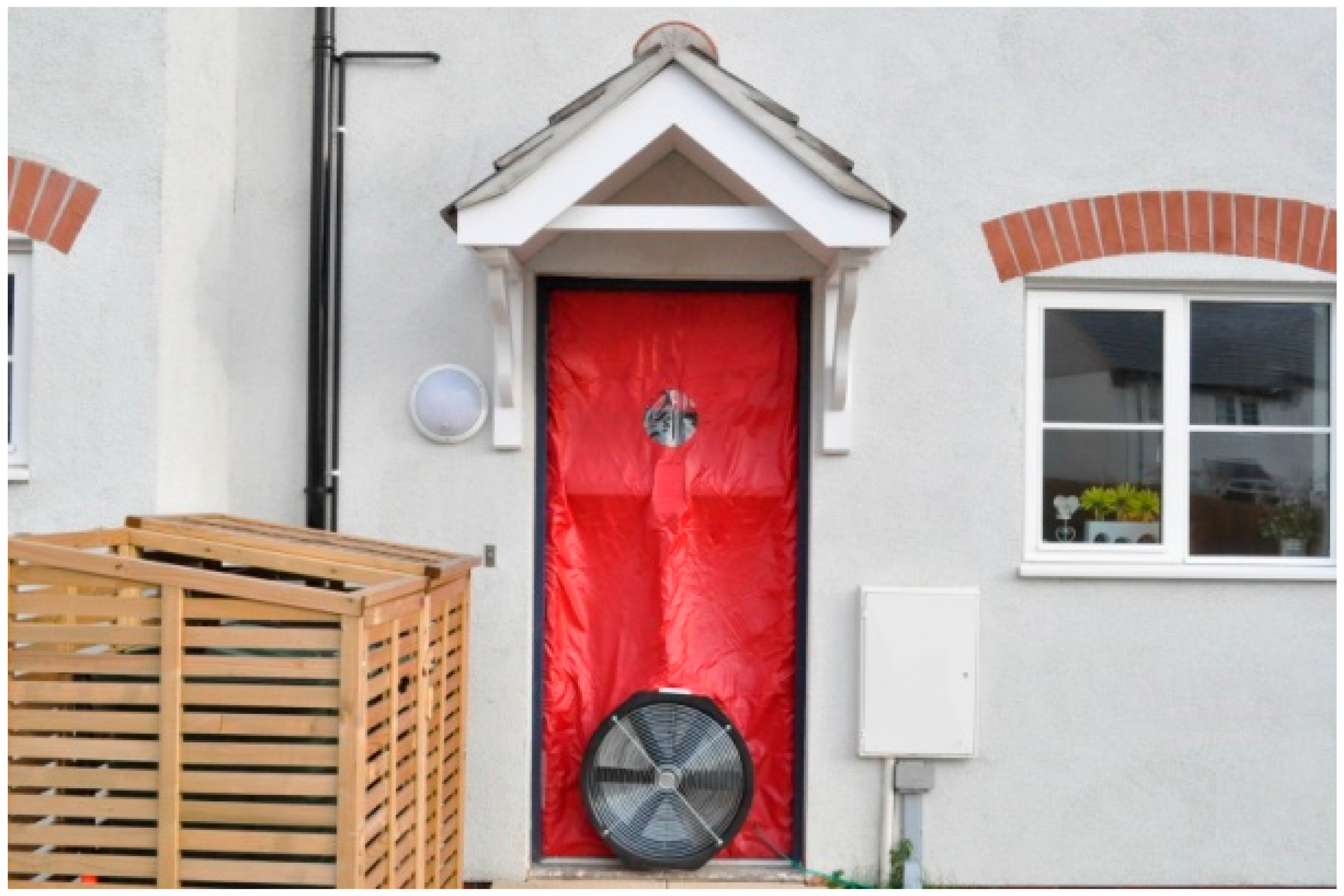
Figure 4.
Co-heating test in the monitored building.
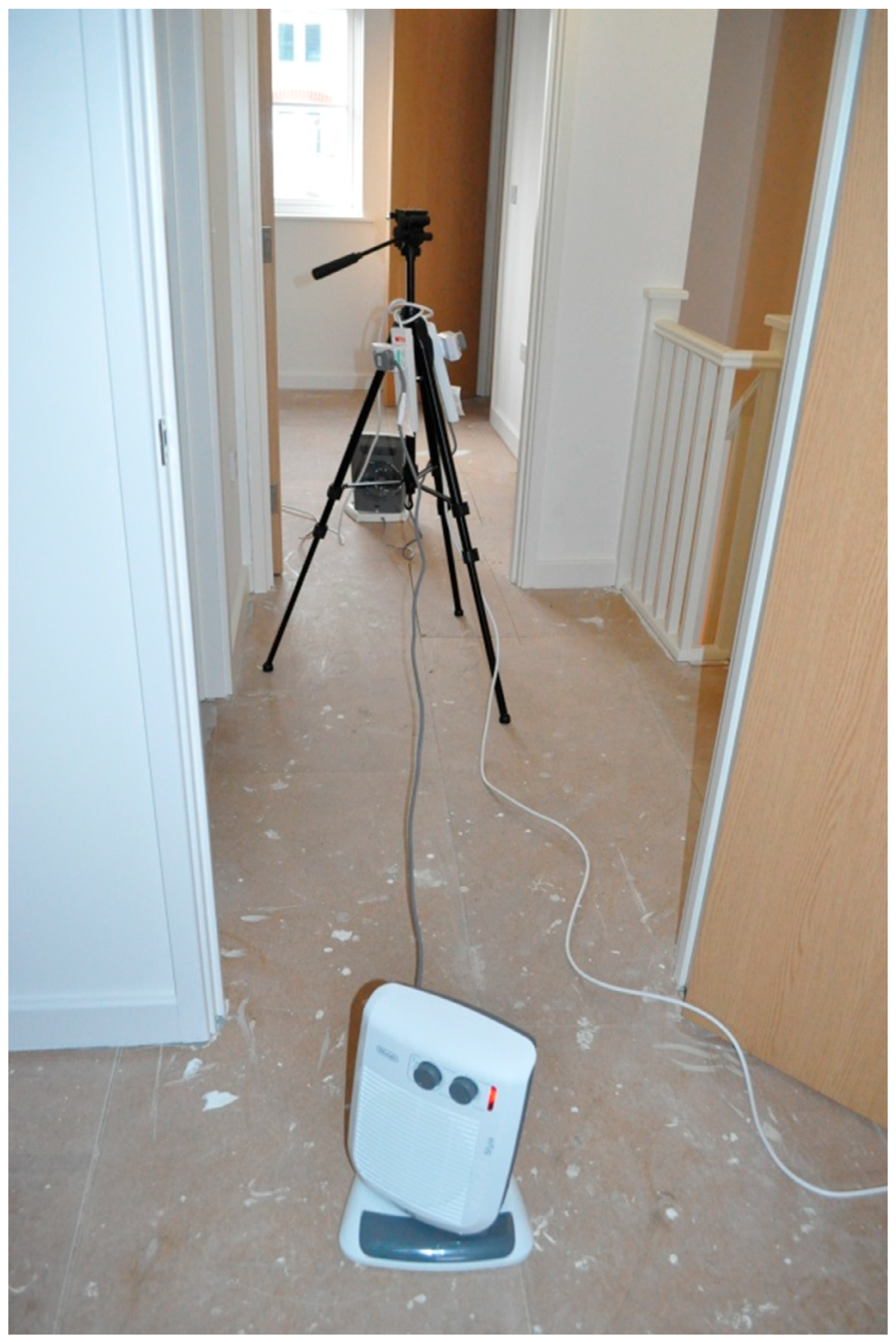
Figure 5.
Air tightness test in the monitored building. (a) External thermal images after the co-heating test—a photo montage representing the thermal image of the house using the ground and floor and first floor thermal images; (b) loft hatch leakage during air tightness test.
Figure 5.
Air tightness test in the monitored building. (a) External thermal images after the co-heating test—a photo montage representing the thermal image of the house using the ground and floor and first floor thermal images; (b) loft hatch leakage during air tightness test.
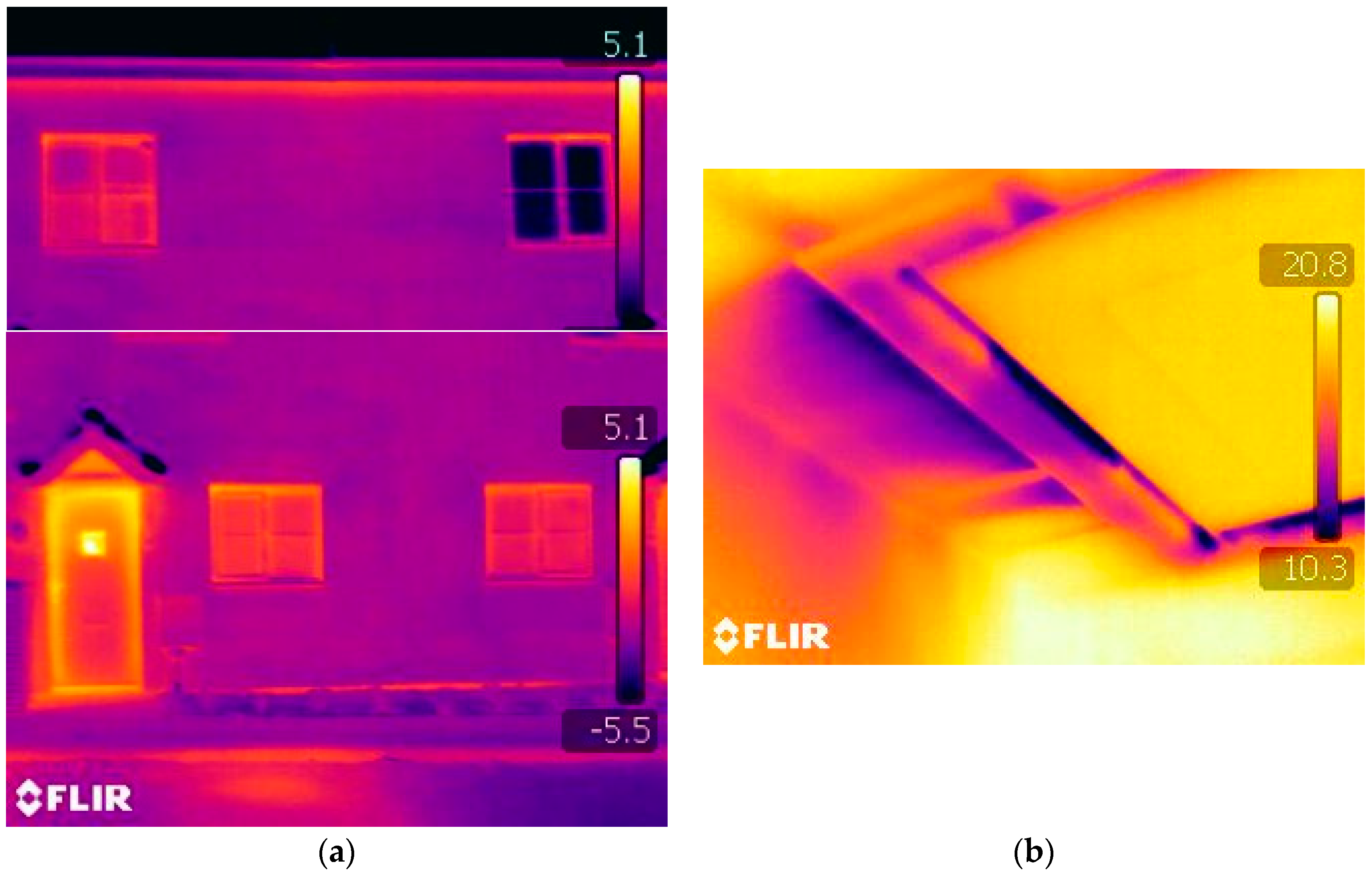
Figure 6.
IES model of the monitored house (monitored house shown in blue, adjacent houses shown in magenta). (a) front view; (b) rear view.
Figure 6.
IES model of the monitored house (monitored house shown in blue, adjacent houses shown in magenta). (a) front view; (b) rear view.

Figure 7.
Comparison between IES temperature, Fourier filtered temperature, and monitored air temperature of the living room.
Figure 7.
Comparison between IES temperature, Fourier filtered temperature, and monitored air temperature of the living room.

Figure 8.
Comparison between IES relative humidity, Fourier filtered relative humidity, and monitored relative humidity of the living room.
Figure 8.
Comparison between IES relative humidity, Fourier filtered relative humidity, and monitored relative humidity of the living room.


| Building Type | Floor Area (m2) |
|---|---|
| Winery | 770 |
| Museum store for artefacts | 870 |
| School building | 180 |
| Pharmaceutical sample storage and archive | 1190 |
| Detached house | 330 |
| Detached house | 413 |
| Warehouse | 7960 |
| Crematorium | 800 |
| Supermarket | 3320 |
| Total | 15,833 |
© 2016 by the author; licensee MDPI, Basel, Switzerland. This article is an open access article distributed under the terms and conditions of the Creative Commons Attribution (CC-BY) license (http://creativecommons.org/licenses/by/4.0/).
Share and Cite
MDPI and ACS Style
Jankovic, L. Reducing Simulation Performance Gap in Hemp-Lime Buildings Using Fourier Filtering †. Sustainability 2016, 8, 864. https://doi.org/10.3390/su8090864
AMA Style
Jankovic L. Reducing Simulation Performance Gap in Hemp-Lime Buildings Using Fourier Filtering †. Sustainability. 2016; 8(9):864. https://doi.org/10.3390/su8090864
Chicago/Turabian StyleJankovic, Ljubomir. 2016. "Reducing Simulation Performance Gap in Hemp-Lime Buildings Using Fourier Filtering †" Sustainability 8, no. 9: 864. https://doi.org/10.3390/su8090864
Note that from the first issue of 2016, this journal uses article numbers instead of page numbers. See further details here.