1. Introduction
The levels of greenhouse gases within the atmosphere have been increasing drastically since the beginning of the industrial revolution. According to the report of the Intergovernmental Panel on Climate Change (IPCC) in 2007, greenhouse gases and carbon dioxide emissions have increased by 70% and 80% from 1970–2004, respectively, with freight transport responsible for approximately one-third of global energy-related carbon emissions [
1]. The United States Environmental Protection Agency (EPA) reported that transportation accounts for approximately 27% of total U.S. greenhouse gas emissions in 2013. Similarly, road transportation produced approximately one-fifth of total carbon dioxide emission in the European Union (EU) where transportation is the only major sector in the EU with continuously rising greenhouse gas emission [
2]. Several nations that attended the 2009 United Nations Climate Change Conference negotiated the terms of carbon control programs designed to protect the environment for the prevention of further damage. The policy makers of several nations have instituted environmental regulations on carbon taxing and carbon trading, as well as imposing carbon caps [
3]. As a result of these legislative actions, a growing number of leading firms, such as Dell, Wal-Mart, LG, Intel and IBM, have engaged in carbon emissions programs. Furthermore, 59% of Financial Times and the London Stock Exchange companies have published targets for reducing greenhouse gases, including proposals for carbon and energy reductions [
4]. According to the operations management literature, environmental issues have been studied from different perspectives. Dekker et al. [
5] addressed decisions on technology selection under both emissions cap-and-trade and emissions tax regulations for a profit-maximizing firm. Benjaafar et al. [
6] analyzed various classical lot-sizing models for single and multiple firms while considering carbon emissions. Jaber et al. [
7] optimized the total cost of a two-level supply chain by including an emission tax and penalty. Absi et al. [
8] presented the extension of the lot-sizing model under different carbon regulatory policies. Nouira et al. [
9] developed an optimization model in which the demand of a product depends on its greenness. Liotta et al. [
10] introduced a carbon emission factor in a transportation optimization model. Hammami et al. [
11] developed a deterministic optimization model that incorporates carbon emissions in a multi-echelon production-inventory model with lead time constraints. Afandizadeh and Abdolmanafi [
12] considered a case study to derive a pricing scheme with environmental equity. We present a bi-objective optimization problem designed for a four-stage production-distribution system with a carbon emission constraint as opening a different perspective compared to the above citations.
The typical production-distribution system involves many stages with various processes that create significant carbon emissions. Therefore, it is important to formulate a new model to study the interactions between multi-stage production-distribution and carbon emissions due to the creation of an immense amount of the chemical from the entire process. The objective of the production-distribution system design problem is to optimize the distribution costs, inventory carrying costs and fixed costs for opening, equipping and managing manufacturing units and distribution centers [
13]. Several companies, including Elkem Silicone [
14] and the Kellogg Company, have achieved substantial cost savings through the optimization of production-distribution systems [
15]. A large body of research focused on the modeling and design of various components of production-distribution problems. Review papers on the topic [
16,
17,
18,
19,
20] summarized the benefits and challenges associated with integrating the overall decision processes while emphasizing the need for practical analytic models and efficient solution methods. One of the major challenges for manufacturers is providing the retailer supply by retaining stockpiles. However, retaining actions for large inventory require increased operational costs. The issue becomes an additional concern over manufacturer’s operations when carbon emissions constraints are introduced to the system. In addition, a stockout may not only result in order cancellations, but may also affect the probability of future customer demand [
21]. Holmes and France [
22] reported that late delivery resulted in enormous fees for the Boeing Company. The company had to lose its customers to Airbus due to delivery delays. KPMG [
23] identified enormous commitments for Food, Drink and Consumer-Goods (FDCGs) companies to satisfy retailer’s product demand. For example, Kroger, a large U.S. grocery chain, applies a flat penalty every time a manufacturer cannot deliver a complete order on time [
24]. Therefore, one of the major challenges for a production-distribution system design problem is eliminating shortages while simultaneously carrying the minimum inventory to reduce carbon emissions. In this study, we propose a bi-objective optimization model that is able to provide an integrated view of strategic operational decisions for the manufacturer to maximize total profits while minimizing shortages with inaccurate information on raw material resources.
Traditional deterministic optimization models are not always suitable for capturing the dynamic behavior of most real-world applications. The production-distribution problems become more challenging when information on raw material availability is imprecise. Fuzzy set theory offers strong analytical support for capturing uncertainty. From the pioneering work from Zadah [
25], fuzzy logic found numerous applications due to its simplicity on implementation, flexibility and tolerant nature for handling imprecise data. Several methods have been addressed to attain fuzzy-efficient solutions for multiple-objective linear programming problems with fuzzy goals. The max-min operator is usually applied because it is easy to compute. The method has been applied to numerous real-world problems, such as market analysis, production planning, environment protection, supplier selection and various related situations [
26,
27,
28,
29,
30,
31]. However, the technique does not guarantee a fuzzy-efficient solution in the presence of multiple unique optimal solutions [
32]. To produce a fuzzy-efficient solution, several researchers have proposed a two-phase approach [
33,
34]. In response, Jimenez and Bilbao [
35] showed that a fuzzy-efficient solution may not be a Pareto-optimal solution when one fuzzy goal is fully achieved. Recently, Wu et al. [
36] proposed a new methodology for solving multiple-objective linear programming problems by using a two-phase approach. They analytically proved that the solution methodology produces a Pareto-optimal solution with additional robust information for decision makers.
In this paper, we propose an application of a two-phase approach to find solutions for the proposed model. We describe a multi-period four-stage production-distribution system design problem composed of units that manufacture products after receiving raw materials from various suppliers and engage distribution centers for collecting and storing products to satisfy demands from retail outlets. The objective is to determine the number of distribution centers in the network, the optimum number of items produced by the manufacturing units, the optimum quantity of products to be dispatched from the manufacturing units to distribution centers and from distribution centers to retail outlets, the optimum inventory of product at distribution centers and manufacturing units, the optimum inventory of raw materials at the manufacturing units and the optimum shortage quantity. The problem contains two conflicting objectives for manufacturers. The first objective is maximizing the total profit, while the second objective is minimizing the amount of the manufacturer’s cumulative shortages. The study advances the existing literature in three important directions. First, the production-distribution planning problem is formulated under a bi-objective framework to maximize profit and minimize cumulative shortages to retain business opportunities, fulfill demand as much as possible and enhance profit simultaneously for the manufacturer. Second, the optimal decision is heavily influenced by the carbon emission constraint where the manufacturer is able to significantly reduce the shortage amount with a bi-objective framework optimization problem. Finally, the study provides meaningful industrial implications and improves the research on sustainability by associating the influence of a carbon emission constraint with a production-distribution planning problem. This paper is organized as follows:
Section 2 introduces the problem description.
Section 3 describes the two-phase approach to find a fuzzy-efficient solution.
Section 4 analyzes the computational results. Lastly,
Section 5 outlines the conclusions and provides suggestions for future research.
2. Model Formulation
In this section, we introduce the nomenclature required for modeling the problem and the mathematical formulation.
2.1. Nomenclature
The following provides the indices used for the model:
| i | index used for manufacturing units, |
| j | index used for distribution centers, |
| k | index used for retail outlets, |
| s | index used for raw materials, |
| t | index used for fixed time periods, |
The following provides the deterministic and fuzzy parameters used for the model:
| unit selling price of the product in the k-th retail outlet |
| unit production cost of the product produced by the i-th manufacturing unit |
| demand of the product in the k-th retail outlet in time period t |
| set up cost for the j-th distribution center |
| unit inventory holding cost in the i-th manufacturing unit |
| unit inventory holding cost in the j-th distribution center |
| unit inventory holding cost of raw material s in the i-th manufacturing unit |
| unit shortage cost of the product for the k-th retail outlet |
| unit cost of raw material type s |
| V | volume of one unit of the product |
| volume of one unit of raw material type s |
| storage capacity available in the j-th distribution center |
| storage capacity of the product available in the i-th manufacturing unit |
| storage capacity of raw material available in the i-th manufacturing unit |
| C | fixed cap on emission initially adhered by the manufacturer for the entire planning horizon |
| unit transportation cost of the product distributed from the i-th manufacturing unit to the j-th distribution center |
| unit transportation cost of the product distributed from the j-th distribution center to the k-th retail outlet |
| requirement of raw material type s to produce one unit of the product |
| unit carbon emission to distribute the product from the i-th manufacturing unit to the j-th distribution center |
| unit carbon emission to distribute the product from the j-th distribution center to the k-th retail outlet |
| unit carbon emission for producing each unit of the product in the i-th manufacturing unit |
| unit carbon emission for keeping each unit of the product in the i-th manufacturing unit |
| unit carbon emission for keeping each unit of the product in the j-th distribution center |
| unit carbon emission for keeping each unit of the s-th type raw material in the i-th manufacturing unit |
| carbon emission due to open and operate the j-th distribution center for entire planning horizon |
| price per unit of carbon offsets |
| imprecise amount of the s-th type raw material available in time period t |
The following provides the decision variables used for the model:
| amount of product distributed from the i-th manufacturing unit to the j-th distribution center in time period t |
| amount of product distributed from the j-th distribution center to k-th retail outlet in time period t |
| amount of raw material type s purchased for the i-th manufacturing unit in time period t |
| amount of product produced by i-th manufacturing unit in time period t |
| shortage amount in the k-th retail outlet in time period t |
| inventory level of product in the i-th manufacturing unit at the end of time period t |
| inventory level of product in the j-th distribution center at the end of time period t |
| inventory level of raw material of type s in the i-th manufacturing unit at the end of time period t |
| amount of additional carbon offset to be purchased by the manufacturer in entire planning horizon |
| binary variable, one if the distribution center j is opened, zero otherwise |
2.2. Multi-Objective Optimization Model
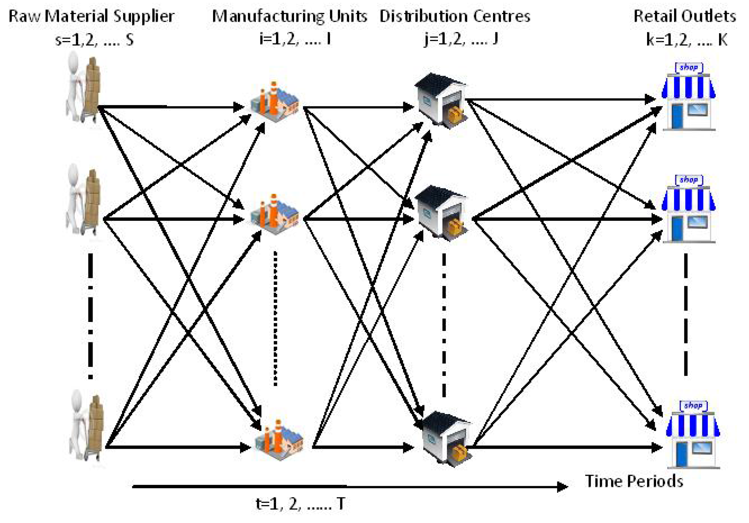
We consider a set of retail outlets (first stage), a set of possible distribution centers (second stage), a set of manufacturing units (third stage) and a set of exclusive raw material suppliers (fourth stage) for modeling our four-stage integrated production-distribution problem.
Figure 1 provides a demonstration of the entire production-distribution system.
The planning horizon consists of multiple time periods where each retail outlet has deterministic and time-varying demand at each corresponding period. Deliveries from raw material suppliers to manufacturing units, from manufacturing units to distribution centers and from distribution centers to retail outlets are direct and instantaneous. Unit transportation costs of each item delivered from the manufacturing units to distribution centers and from distribution centers to retail outlets are given for each period with negligible ordering cost. To incorporate carbon emission concerns, we consider a situation where the manufacturer must comply with a fixed cap on emission over the entire planning horizon. We also assume that the manufacturer is allowed to invest in carbon offsets to reduce carbon caps. We assume that the carbon emission parameters are readily available [
3]. Shortages are allowed in each retail outlet, and the manufacturer can completely backlog the shortage amount from the previous period. Each supplier’s capacity is imprecise. We simultaneously optimize two conflicting objective functions for the manufacturer. The first objective function represents the profit for the manufacturer, and the second objective function represents the cumulative shortage amount for the entire planning horizon. Our aim is to determine:
The flow of product from manufacturing units to retail outlets
The amount of raw materials to be procured
The number of distribution centers
The shortage quantities in all retail outlets
The inventory for manufacturing units and selected distribution centers at the end of each period
The inventory of raw materials for manufacturing units at the end of each period
The amount of carbon offset to which the manufacturer adheres for the entire planning horizon
Equations (1)–(14) present the objective functions, functional and operational constraints and restrictions on the decision variables for the proposed fuzzy bi-objective optimization model.
subject to:
Equation (1), the first objective function, maximizes the total profit for the manufacturer gained from selling the final product subtracted by the production cost, transportation cost from manufacturing units to distribution centers and from distribution centers to retail outlets, the cost of raw materials, inventory holding cost at manufacturing units and distribution centers for the finished product, inventory holding cost for raw materials at manufacturing units, setup cost of each distribution center, backorder cost at retail outlets and carbon offsets cost. Equation (2), the second objective function, minimizes the total cumulative shortages for the entire planning horizon. Constraints (3)–(6) represent the balance equations for the raw materials at the manufacturing units, product inventory at manufacturing units, product inventory at potential distribution centers and shortages at retail outlets. Constraints (7) represent the impreciseness of the raw material’s availability information. Constraints (8) limit the volume of the product dispatched to potential distribution centers to the total storage capacity. Constraints (9)–(11) enforce the inventory levels of raw material by ensuring the product inventory at potential distribution centers and manufacturing units to not to exceed their respective capacities. Constraints (12) restrict the production volume, which must be less than the total storage capacity of the manufacturing units. Constraints (13) represent emission constraints. Constraints (14) ensure that decision variables for the open-close status for all distribution centers are binary, whereas other variables are non-negative. Note that the indices t and are used respectively to represent the present period and the previous period.
The complexity of the proposed optimization model can be expressed as a function of problem size affected by the set of raw material suppliers, manufacturing units, distribution centers and retail outlets. The model is composed of decision variables and constraints, where are fuzzy.
3. Solution Procedure
The developed model from
Section 2 is a bi-objective optimization problem with fuzzy constraints. A two-phase approach [
36] is used to obtain a fuzzy efficient solution. The following are several useful definitions for the context.
Definition 1:
A multiple objective optimization problem can be represented as follows:
where “opt” denotes minimization or maximization;
are the decision variables;
are multiple objectives to be optimized;
includes the system constraints.
Definition 2:
A decision plan is said to be a Pareto optimal solution to the multiple objective optimization problem if there does not exist another , such that for all k and for at least one s.
Definition 3:
A decision plan is said to be a fuzzy-efficient solution to the model if there does not exist another , such that for all k and for at least one s.
For multi-objective optimization problem, not all objective functions will simultaneously derive optimal values. In order to overcome such a case, finding an optimal solution for the problem requires Pareto optimality, which prevents the improved solution for an individual objective from worsening one or more other objectives. However, fuzzy-efficiency may not guarantee Pareto-optimality if the decision maker must choose a compromised solution according to each objective’s appropriate aspiration levels for the achievable goals in the presence of several objective functions. In these circumstances, fuzzy-efficiency does not guarantee Pareto optimality. Because the proposed production-distribution planning problem contains imprecise raw material resources (Constraints (7)), we use the two-phase approach proposed by Wu et al. [
36]. If we assume that
has the minimum resource
with tolerance
(
), then the linear membership functions,
,
and
for the fuzzy constraints can be formulated as follows:
We also formulate linear membership functions featuring both the continuously increasing property of the maximization objective function (
) and the continuously decreasing property of the minimization objective function (
). For the maximization objective function:
For the minimization type objective function:
where the possible range for the
i-th objective
, (
i= 1, 2) is defined by the decision maker. The range is constructed from the solution of the problem by incorporating only one objective function while ignoring the other objective function as subject to the set of functional constraints and fuzzy constraints of
and
, respectively.
Figure 2a shows a graphical representation for a maximization type of a membership function, while
Figure 2b shows a graphical representation for a minimization type of a membership function.
Under the two-phase approach, we need to find the optimal solution for the following problem in Phase I:
Membership functions in the two-phase approach do not have an upper bound unlike the conventional max-min operator approach. If the value of the membership function is restricted by an upper bound, the objective function may not attain the lowest or highest possible value because the fuzzy goals are set by the decision maker subjectively. The two-phase approach provides the flexibility to reach optimal goals by relaxing this constraint in Phase I. Finally, we need to find the solution for the following problem in Phase II:
where
is the optimal value of
λ obtained in Phase I.
Note that if and , then there are no solutions with better efficiency for the model under Phase I. If for some r, the solution obtained from Phase II is more efficient compared to the solution obtained from Phase I, and the decision maker would be able to obtain information for achieving subjective goals.
Proposition 1: If
is an optimal solution of problem defined for Phase II, then
is a Pareto-optimal solution [
36].
4. Computational Experiments
To illustrate the proposed model and the effectiveness of the solution procedure, we consider a production-distribution network with two manufacturing units [
,
], three potential distribution centers [
,
,
] and six retail outlets [
,
,
,
,
,
]. Additionally, each product requires three different raw materials that are provided by three different suppliers [
,
,
]. We use a time horizon consisting of three periods. The manufacturer sells the product to retail outlets at a price of $25 and with a corresponding shortage cost of $1. We further assume that the initial inventory levels at various stages are:
;
;
; and
. All other parameters are defined in
Table 1,
Table 2 and
Table 3. The optimal solutions are obtained from a computer with an Intel core i5 2.5 GHz CPU and a Windows 7 operating system. We solve the problems using IBM ILOG CPLEX Optimizer.
Table 4 and
Table 5 show the ideal solutions for the objective functions (1) and (2), respectively, subject to the set of functional and operational constraints at
.
Table 4 shows the ideal solution for problem with objective function (1) with values $11,638.52, 285 units and 29.41 kg for the optimal profit of the manufacturer, amount of cumulative shortages and carbon offsets, respectively. The above scenario only uses the second distribution center. In our model,
represents the shortage amount of the
k-th retail outlet for time period
t. The demand for the first retail outlet in the first time period is 45 units. However, 15 units are delivered from the second distribution center. Therefore, the total shortage is 30 units. The demand for the first retail outlet in the second time period is 40 units. However, finished products are not supplied during this period. Therefore, the amount of combined shortages for the first retail outlet is 70 units at the end of the second period. Similar to the case of having limited available supply for
in the second time frame, finished products are not supplied during the third time frame despite the presence of the demand of 40 units. Therefore, the amount of cumulative shortages becomes 110 units. In the sixth retail outlet, the shortage amount for the second period is 25 units, and demand for the third period is 65 units. Because 90 units are supplied during the third period, no shortages occur in the third time period.
Table 5 shows the ideal solution for problem with the objective function (2). The solution holds noticeably different characteristics compared to the previously-explained ideal solutions from the first scenario. The amount of shortage for the entire planning horizon becomes zero with corresponding optimal profit and carbon offsets as $7525.84 and 176.25 kg, respectively. Moreover, the manufacturer must maintain a large inventory of both raw material and finished product to fulfill the future demand. The scenario creates high carbon offsets and comparatively low profits. The manufacturer needs to use the second and third distribution centers in the planning horizon. Furthermore, the second objective function’s optimal distribution schedule’s characteristic is significantly different compared to the first objective function’s optimal distribution schedule’s characteristic. The ideal solutions for the objective functions subject to the set of functional constraints and operational constraints at
maximizing the profit and minimizing the total cumulative shortage are shown in
Table 6 and
Table 7, respectively.
Table 6 shows the ideal solution for the problem with the objective function (1) with values $11,516.84, 305 units and 28.41 kg for the optimal profit of the manufacturer, total cumulative shortages and carbon offsets, respectively. Compared to the solution obtained from using
,
’s solution shows an increased optimal shortage amount and decreased profit. The observation implies that strict resource constraints significantly affect the ideal solution for the problem. Additionally, the manufacturer should maintain inventory for raw materials.
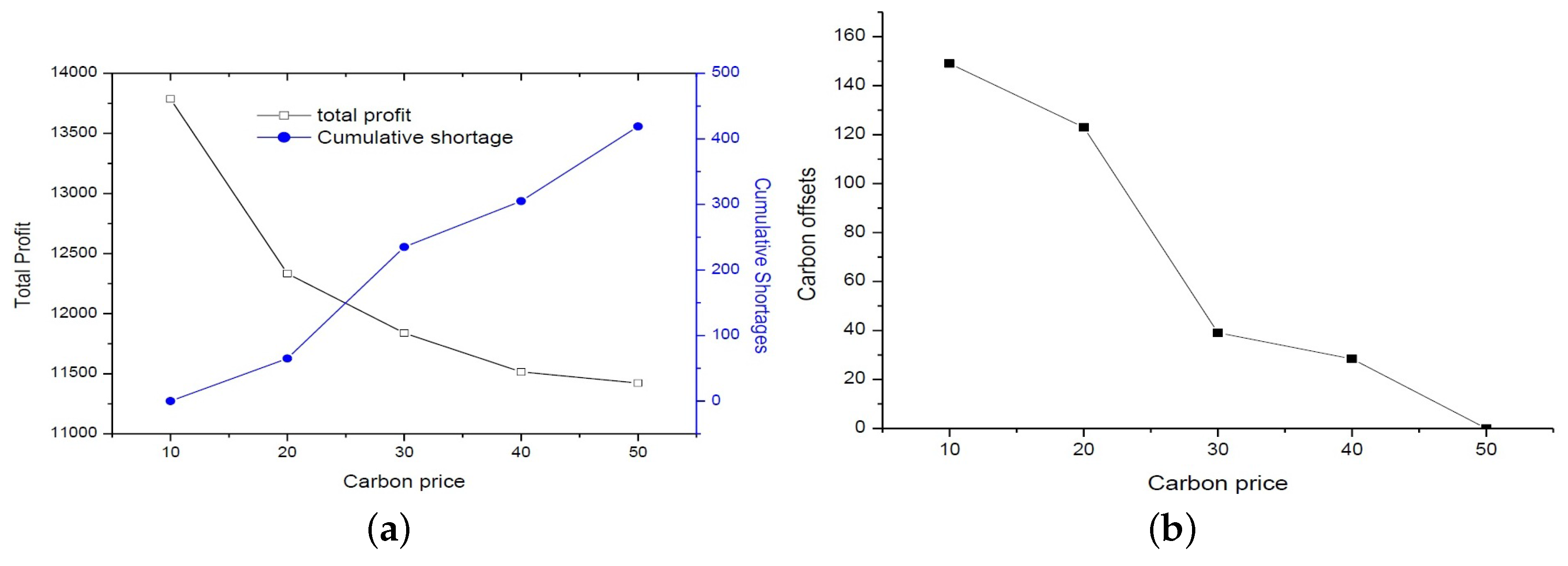
Table 7 represents the ideal solution for the problem with the objective function (2) with $7090.51 and 181.15 kg as the optimal profits and carbon offsets, respectively. The manufacturer is able to fulfill the demand for all retail outlets at the expense of the profit. In addition, a large deviation in carbon offsets is observed. The results of the sensitivity analysis of the effect of carbon price at
on the objective function (1) are given in
Figure 3a,b.
Figure 3a shows an exponentially decreasing manufacturer’s optimal profit and an exponentially increasing amount of cumulative shortages. Similarly,
Figure 3b shows a decreasing amount of carbon offsets as the
increases. Therefore, the manufacturer should minimize the shortage to retain business opportunities when facing the presence of the emission constraint.
Figure 4 shows the results from sensitivity analysis on the objective function (1) affected by the effects of shortage cost at
.
From
Figure 4, we can conclude that the amount of carbon offsets and the total profit are sensitive to the shortage cost. As the shortage cost increases, the manufacturer profit decreases, and the amount of carbon offsets increases. Through examining the above ideal solutions and the sensitivity analysis results, we are able to conclude that a trade-off exists between the objective functions. Furthermore, the solutions are highly sensitive to the tolerance margins
, (i.e., the subjective estimation of available resources). The result motivates us to find a solution to the proposed bi-objective optimization problem by using a two-phase approach in which the subjective goals of decision makers are unrestricted. Under the two-phase approach, the value of the membership functions can be larger than one. Therefore, the decision makers can evaluate whether the fuzzy goals of the objective functions are overestimated and compute the possible amount of overestimation.
Table 8 and
Table 9 show the fuzzy-efficient solutions obtained from solving (15) and (16).
From
Table 8, we see that the total amount of shortage is reduced to 81 units. The optimal profits and additional carbon emissions are $10,634.45 and 104.59 kg, respectively. Therefore, the obtained solution is a Pareto optimal solution. Finally, according to
Table 9, the solution obtained in Phase II indicates the reduced shortage amount of 59 units. The computation time for solving the final problem is 0.109 s. The demand for the first retail outlet in the second time period is 40 units. However, 31 units are delivered from the second distribution center and results in a total shortage of nine units. The demand for the first retail outlet in the third time period is 40 units. However, the finished product is not supplied during the period. Therefore, the amount of combined shortages for the first retail outlet becomes 49 units at the end of the third period. The corresponding optimal profits and additional carbon emissions are $10,766.12 and 109.03 kg, respectively. By comparing the final solution with the solution given in
Table 8, we conclude that the manufacturer can reduce the shortage amount by 79.29% at the expense of 7.49% profit.
5. Conclusions and Future Research
In this study, we propose a four-stage production-distribution planning problem under a carbon emission restriction and imprecise information on raw material resources. A fuzzy bi-objective optimization problem is formulated for determining the trade-off between the optimal profits and shortages. The problem is solved with a two-phase solution approach to find the fuzzy-efficient solution for the manufacturer. The computational experiments are performed for analyzing, validating the model and determining whether the solution approach is able to provide the flexibility required for obtaining a Pareto-optimal solution in a bi-objective decision making environment.
The results in this paper have important managerial implications. First of all, minimizing shortages is crucial for fulfilling the present demand and retaining future business opportunities. The study showed that the carbon penalty increases the amount of shortages, which would decrease the manufacturer’s profit. However, under the bi-objective optimization formulation, operational adjustments can lead to significant reductions in emissions and shortages without considerably decreasing the profit. The manufacturer can reduce the business risk even in the absence of long-term accounts by ensuring the fulfillment of orders for retailers and keeping the market share. Second, the optimal solution obtained by using the two-phase approach always provides a desired Pareto-optimal solution along with additional information for achieving objective goals despite the difficulty of setting goals under the multi-objective optimization framework due to imprecise information on raw material resources. Finally, the study provides important industrial implications. The optimal decision for a production-distribution planning problem under an emission constraint should be considered with a bi-objective formulation, which contributes to enhancing business opportunities under environmental regulations by allowing decision makers to fulfill demand and maximize profit.
Research on this problem can be extended in several ways. For example, assumptions on deterministic demand can be relaxed by incorporating fuzzy or stochastic demand. Future research may incorporate the selection problem where each supplier can sell more than one raw material. Researchers may want to generalize the solution procedure for further application on large-scale problems. Additionally, the study can be extended to analyzing the problem with a supply chain framework where operations at each state are controlled by different members for profit maximization and emission minimization for all corresponding controlling members.


