Article

The Shortest Path Problems in Battery-Electric Vehicle Dispatching with Battery Renewal

1
School of Economics and Management, North China Electric Power University, Beijing 102206, China
2
California PATH, University of California, Berkeley, Richmond, CA 94804, USA
*
Author to whom correspondence should be addressed.
Sustainability 2016, 8(7), 607; https://doi.org/10.3390/su8070607
Submission received: 26 April 2016 / Revised: 13 June 2016 / Accepted: 22 June 2016 / Published: 28 June 2016
(This article belongs to the Section Energy Sustainability)

Abstract

:
Electric vehicles play a key role for developing an eco-sustainable transport system. One critical component of an electric vehicle is its battery, which can be quickly charged or exchanged before it runs out. The problem of electric vehicle dispatching falls into the category of the shortest path problem with resource renewal. In this paper, we study the shortest path problems in (1) electric transit bus scheduling and (2) electric truck routing with time windows. In these applications, a fully-charged battery allows running a limited operational distance, and the battery before depletion needs to be quickly charged or exchanged with a fully-charged one at a battery management facility. The limited distance and battery renewal result in a shortest path problem with resource renewal. We develop a label-correcting algorithm with state space relaxation to find optimal solutions. In the computational experiments, real-world road geometry data are used to generate realistic travel distances, and other types of data are obtained from the real world or randomly generated. The computational results show that the label-correcting algorithm performs very well.

1. Introduction

Recently, aimed at reducing vehicle emissions and greenhouse gases, more and more electric transit buses and delivery trucks have been used in personal travel, public transit, home deliveries from grocery stores, postal deliveries and courier services. For example, electric motorcycles or scooters have been promoted through incentive programs in Taiwan. UPS began using electric vehicles in their fleet as early as 1933, and now almost 2000 electric delivery trucks have been used [1]. More than 80 electric transit buses were used in the World Expo 2010 Shanghai [2]. As a benchmark city of electric vehicle demonstration application in China, Beijing released the Beijing electric vehicle promotion application action plan (2014–2017) in June, 2014 [3]. Although electric vehicles produce zero emissions, a fully-charged battery only allows running a limited operational distance. The limited short range may not be a problem for commute drivers in an urban area. It will have great impacts on the applications of vehicle scheduling and routing. In order to make electric vehicles service for a whole day, the battery near depletion can be either quickly charged or exchanged with a fully-charged one at a battery service station. Therefore, the problem of electric vehicle dispatching with battery renewal falls into the category of the resource-constrained shortest path problem.
The resource-constrained shortest path problem consists of determining the lowest-cost path from an origin node to a destination node on a network, such that resources consumed along the path are no more than specified values. Some typical examples of resources include maximum daily working hours, vehicle capacity, fuel tank size and maximum traveled distances. The resource-constrained shortest path problem has significant applicants in transportation, such as in vehicle scheduling with time windows [4], vehicle routing with time windows [5], transit crew scheduling [6] and airline crew pairing [7]. In these applications, the resource-constrained shortest path problem often appears as a sub-problem in the context of column generation. One critical component of an electric vehicle is its battery. Unlike the resources previously mentioned, a battery can be quickly charged or exchanged with a fully-charged one before it runs out. Such an aspect results in the shortest path problem with resource renewal, which will be investigated in this paper.
The resource-constrained shortest path problem may be classified into two types. In the first type, either the problem is based on an acyclic network, or although the underlying network is cyclic, there are no negative cost cycles (e.g., all arcs have positive costs). Solution approaches include branch-and-bound [8], label setting [9], label setting with preprocessing [10], K-shortest path enumeration [11,12] and Lagrangian relaxation with robust shortest path enumeration [13]. In the second type, there are negative cost cycles in the underlying network. If no cycles are allowed in the shortest path, such a problem is called the elementary shortest path problem with resource constraints. Solution approaches include branch-and-bound [8], label correcting [14], bi-directional label correcting [15] and label correcting with state space relaxation [16]. A relaxed version allows the existence of cycles in the shortest path. Solution methods are mainly based on dynamic programming with the strategies of two-cycle elimination [5,17], k-cycle elimination [18] and a combined (k, 2)-loop elimination [19]. Both types of resource-constrained shortest path problems are NP-hard [20]. The literature about the electric vehicle routing problem is focused on refueling station location [21,22], battery swapping or charging replenishment [23,24] and the electric traveling salesman problem [25] or the electric vehicle routing problem [26,27,28].
In this paper, we consider the shortest path problems in two types of electric vehicles with battery renewal: electric buses and electric trucks. The problem on electric buses is defined as follows: given an origin and a destination depot, a set of scheduled trips with starting and ending times, the travel distance between two locations, the maximal range of the electric bus before battery renewal and the cost between two nodes, find the shortest path from the origin depot to the destination depot. The problem on electric trucks is similar, but with additional constraints: the service has flexible time windows and demand, and the truck has limited capacity.
The contributions of this paper are as follows. First, we model the shortest path problem in two important applications: (1) electric transit bus scheduling and (2) electric truck routing with time windows. We propose integer programming-based formulations. Second, we develop a dynamic programming-based algorithm to find optimal solutions for these emerging shortest path problems. Third, we conduct the extensive computational experiments in the context of real-world settings: the travel distance is obtained from real-world road geometry data; the battery service time and operational distance are obtained from real-world experiences; and the unit electricity cost is estimated based on real-world testing reports. We also compare the computational time with CPLEX.
The rest of this paper is organized as follows. Section 2 models the shortest path problems with battery renewal. Section 3 presents the label-correcting algorithm. Numerical studies are presented in Section 4. Section 5 concludes the paper and describes future research directions.

2. The Shortest Path Problems in Electric Vehicle Dispatching

In this section, we first model and formulate the shortest path problem in electric transit bus scheduling with battery renewal, where the underlying network is acyclic. We then model and formulate the shortest path problem in electric truck routing with battery renewal and time windows, where the underlying network may contain negative cost cycles.

2.1. The Shortest Path Problem in Electric Transit Bus Scheduling

Heavy-duty diesel trucks and buses generate more than 45% of the nitrogen oxide and 75% of the particulate matter [29]. In contrast, electric transit buses have a unique advantage: zero emissions. The use of electric buses in transit service may date back to the 1990s in Santa Barbara, California [30], and Chattanooga, Tennessee [31], with the main purpose of reducing vehicle emissions in downtown areas. Electric buses were used at a large scale during the Beijing Summer Olympics [32] and World Expo 2010 Shanghai [2]. It was reported in [33] that nine electric buses have been used in Seoul. In Los Angeles, Foothill Transit has already used a number of electric buses in service with a future goal of a 100% clean-fuel fleet [34].
A major problem of electric buses is the restricted operational distance caused by the limited battery capacity. For example, a bus with 22 to 25 seats can run 60 to 90 km in Chattanooga before the battery runs out [31]. In the Beijing Olympics, the maximum operational distance is 130 km [32]. The electric buses servicing Seoul can run 80 km [33]. In the Foothill Transit of Los Angeles, a fully-charged battery can propel the bus for 3 h [34]. In [35], certain specifications of electric bus engines are listed. The use of an air conditioner has a great impact on the operational distance. The United Nations Environment Programme [2] reported that the maximum distance was 150 km with an air conditioner on and 250 km with an air conditioner off in the Shanghai World Expo. In order to overcome the short operational distance, a battery near depletion can be charged or exchanged with a fully-charged one at a battery service station. The fast charge is used in Seoul and Los Angeles; the charging time is from 20 to 30 min in Seoul [33] and about 10 min in Los Angeles [34]. Battery exchange has been employed in Tennessee [31], Beijing [30] and Shanghai [36]. The time of each battery exchange is 10 to 15 min in Tennessee [31].
Both battery charging and exchange are generally accomplished at a battery management station, which has limited service spaces. If a bus arrives at a battery station without any available space, the bus has to wait. We define a maximum waiting time at each battery station in order to avoid unnecessarily long waiting. The capacity of battery stations cannot be violated at any moment. We use a discretization approach to handle this requirement. For each trip, the earliest service start time at a battery station is the arrival time, and the latest service start time is the arrival time plus the maximum waiting time. We then sample the start time range and generate certain discretized nodes. The discretization is applied to all of the trips. The discretized nodes are called time-expanded station nodes, each of which corresponds to a battery service station at a specified time. Such a discretization technique has been widely used in the single-track train scheduling problem with limited spaces at a terminal (e.g., see [37]) and transit bus scheduling with the maximum route distance constraint for compressed natural gas, diesel or hybrid-diesel buses [38].
We now formally define the shortest path problem. The parameters that will be used in the paper are listed as follows.
B the set of available battery stations;
Tb the set of time-expanded station nodes associated with b B ;
T = U b B T b the set of all time-expanded nodes;
at service starting time;
Ut the battery service (swapping or charging) time at node t T ;
at + Ut service ending time;
S the set of service trips;
as starting time, s S;
Us the service duration, s S;
o the origin depot;
d the destination depot;
D the maximum distance that a fully-charged battery allows;
dij the travel distance from i {oT}, or the ending point of trip i S to j {dT}, or the ending point of trip j S; the trip service distance is included if j S;
tij the travel time from i {oT}, or the ending point of trip i S to j {dT}, or the ending point of trip j S;
A the set of arcs, including the following arcs: (1) arcs from o to i S; (2) arcs from i ST to d; and (3) arcs from i ST to j ST if ai + Ui + tijaj and at least one of i and j belongs to S;
c ¯ j i the arc cost, often defined as the operational cost; if the shortest path appears as a sub-problem in column generation or Lagrangian relaxation, c ¯ j i is defined as a function of the operational cost of arc ji and linear or Lagrangian dual variables; it is worthy to mention that the underlying network is acyclic because the starting times of all nodes in ST are fixed.
The decision variables are defined as follows.
xji a binary variable; xji = 1 if a vehicle is assigned to node i directly after node j;
gs a continuous variable that indicates the accumulative distance traveled to the ending point of trip s S since the latest battery renewal.
The shortest path problem in electric transit bus scheduling with battery renewal is formulated in Table 1.
The objective is to minimize the total cost. Constraint (a2) ensures sending a unit flow; Constraint (a3) forces receiving a unit flow; and Constraint (a4) is flow conservation. Constraint (a5) determines the accumulative distance traveled since the latest battery renewal. Constraint (a6) sets the accumulative distance as zero at battery stations and the origin depot. Constraint (a7) forces that the maximum route distance restriction is satisfied.
If a sufficiently large penalty is imposed for each arc ji with i T, the problem becomes the resource-constrained shortest path problem, which is NP-hard [20]. Therefore, the shortest path problem in electric transit bus scheduling is NP-hard.

2.2. The Shortest Path Problem in Electric Truck Routing with Time Windows

The rapid development of online retailing has brought the huge demand of last-mile delivery of parcels. The application of electric trucks will offer great potential to reduce greenhouse gas emissions. FREVUE (Freight Electric Vehicles in Urban Europe) provides evidence on how innovative solutions using electric freight vehicles can help to achieve emission free city logistics. It reports that the electric vehicles should be used in a two-phase delivery network [25], which has been widely adopted by big online retailers, e.g., yhd.com and jd.com in China. In the network, conventional trucks first send parcels to delivery terminals, and later, the electric vehicles finish the last-mile deliveries to customers. A number of electric trucks have already been used in a major shipping company in order to reduce emissions and maintenance costs [1]. It was also reported in 2011 [39] that UPS agreed to purchase 100 electric vans for use in California. Major car manufacturers also produce electric shuttles now. For example, Ford Motor has proposed a type of electric van, named the Ford Transit Connect [40]. Electric delivery trucks also face the restriction of the maximum operational distance. For example, the maximum operational distance of Ford Transit Connect is 120 km [40], and the new trucks that UPS agreed to buy can run about 140 km after a full battery charge [39]. It was reported that it can take six to eight hours for Ford Transit Connect to have a full charge [40].
In the current practice, electric trucks generally serve a relatively short and direct route [39] and do not have the problem of battery depletion. However, in order to use electric trucks at a large scale, the charging time has to be significantly reduced (e.g., using direct current charging) or a battery exchange station has to be built. Although we did not find reports on battery exchange for electric trucks, it can be expected that battery exchange facilities will be constructed in the future. Such construction may be benefited by financial incentives from governments and air-quality management districts. In fact, seven millions incentives were obtained when UPS agreed to buy electric vans [39]. We will assume that at least one battery station has been constructed for battery exchange or fast charging. Similarly, a battery service station can simultaneously serve a limited number of electric trucks.
We now define the shortest path problem formally.
S the set of the customers;
[ai, bi] the time window of customer i S;
vi demand of each node i S;
Ui service duration of each node i S;
D the maximum operational distance;
V the vehicle capacity;
dij the travel distance between each pair of locations;
tij the travel time between each pair of locations;
A the set of arcs, including the following arcs: (1) arcs from o to i S; (2) arcs from i ST tod; and (3) arcs from i ST to j ST if ai + Ui + tijbj and at least one of i and j belongs to S;
c ¯ j i the arc cost, often defined as the distance cost and may include linear or Lagrangian dual variables if the shortest path appears as a sub-problem in column generation or Lagrangian relaxation;
B the set of available battery stations;
Tb the set of time-expanded station nodes associated with b B. This is determined in a similar way for electric bus scheduling: for each customer i S, we determine its earliest and latest service start time at a battery station. The earliest service start time equals ai plus Ui plus the travel time to the battery station, while the latest service start time equals bi plus Ui plus the travel time to the station plus the maximum waiting time. The discretization is then used to sample the start time range, and the time-expanded station nodes are generated. T = U b B T b is then the set of all time-expanded nodes, each of which corresponds to a battery station with specific starting time ai = bi, i T.
Unlike the electric bus scheduling problem, the electric truck routing problem may be based on an underlying network with negative cost cycles if the width of time windows is large.
Decision variables are defined as follows.
si the service start time at node i;
xji, gs the same definition as in electric bus scheduling.
The shortest path problem in electric truck routing with the time windows, vehicle capacity and battery renewal is then formulated in Table 2.
The objective (b1) is to minimize the total cost. Constraints (a2) to (a7) have the same meanings as in electric bus scheduling. Constraints (b3), (b4) and (b5) ensure that the requirement of starting time is satisfied. Constraint (b6) guarantees that the vehicle capacity is not violated.
If D is set as a sufficiently large value, the problem becomes the shortest path problem with time windows, which has been proven to be NP-hard in the strong sense [40]. Therefore, the shortest path problem in electric truck routing is NP-hard.

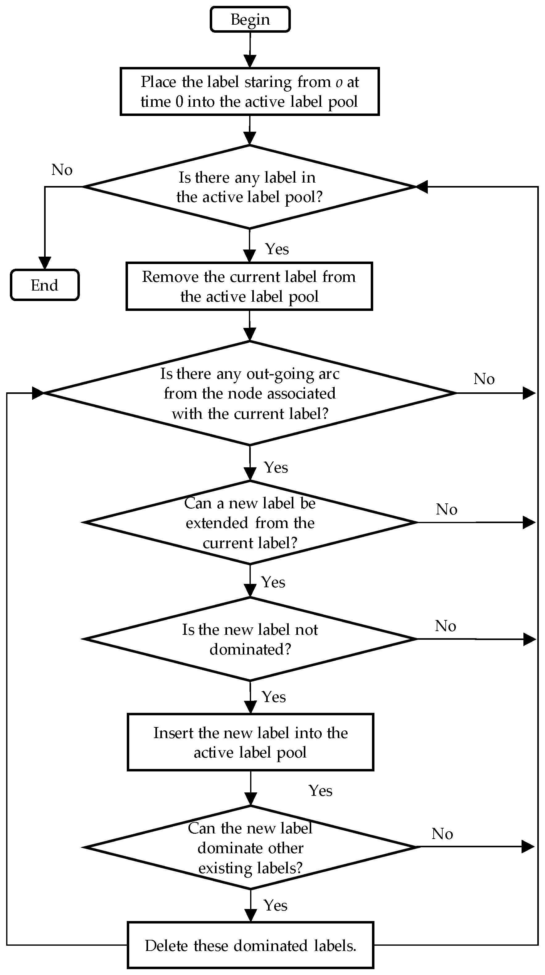
3. The Label-Correcting Algorithm

In this section, we present a label-correcting algorithm to solve the proposed shortest path problems. As discussed in Section 1, preprocessing and K-shortest path enumeration have been successfully used in the resource-constrained shortest path problem without negative cost cycles. Although the underlying network for electric bus scheduling does not contain negative cost cycles, it is difficult to employ these approaches due to the battery renewal. In this paper, we develop a unified label-correcting algorithm to find the optimal elementary shortest paths for both the electric bus scheduling and electric truck routing problems. The details of the label-correcting algorithm (LC) are provided in Figure 1. After the algorithm is finished, an optimal elementary path will be outputted.
Two major operations in the label-correcting algorithm are label extension and label dominance. Label extension is critical to ensure the solution feasibility, while label dominance is crucial to algorithm efficiency. Dominated labels can be deleted from the label pool.

3.1. The Label Operations for Electric Bus Scheduling

The label operations are relatively simple for electric bus scheduling due to an acyclic underling network and fixed service start times. In the extension context (state space), each state can be represented by label (i, g), where i is the last reached node and g the accumulative traveling distance since the last battery renewal. c ¯ (i, g) represents the accumulative cost of label (i, g) since leaving from the depot.
The first label in the extension space is (o, 0), which means that the vehicle starts from the depot with distance zero and cost zero. Label (i, g) can be extended to label (j, g ¯ ). If g + dijD. Additionally, g ¯ can be determined by a rule: g ¯ = 0 if j T, and g ¯ = g + dij otherwise. For the label dominance relationship, let label (i; g) and label (i, g ¯ ) be two paths to node i. We define label (i, g ¯ ) to be dominated by label (i, g) if c(i, g) ≤ c(i, g ¯ ) and g g ¯ .

3.2. The Label Operations for Electric Truck Routing

The label operations are much more complicated for electric truck routing due to the existence of negative cost cycles and additional constraints on the vehicle capacity and time windows. Each label is now defined as (i, g, s, v, R), where s represents the earliest time when service can commence at i and v represents the accumulative demands at i. R is a binary resource vector to indicate if every node i S is visited [8], aimed at avoiding negative cost cycles: initially, all of the positions in R are set to zero; and if a node is visited, the corresponding position in R is set to one. It is not needed to keep track of visiting information for time-expanded station nodes in T. Due to the fixed service starting time, such nodes cannot be visited more than once in a feasible solution. The cost of label (i, g, s, v, R) is c ¯ (i, g, s, v, R).
The first label in the extension is (o, 0, 0, 0, R) with Ri = 0, i S. Now, consider that label (i, g, s, v, R) is extended to label (j, g ¯ , s ¯ , v ¯ , R ¯ ). The extension is feasible if: (1) g + dijD; (2) s + Ui + tijbj; (3) v + vjV; and (4) j has not previously been visited (Rj = 0). If feasible, label (j, g ¯ , s ¯ , v ¯ , R ¯ ) is determined as follows: g ¯ = 0 if j T, and g ¯ = g + dij otherwise; s ¯ = max{s + Ui + tij, aj}; v ¯ = v + vj; and R ¯ k = Rk if kj, and R ¯ j = 1. Then, we discuss the label dominance. Consider that both label (i, g, s, v, R) and label (i, g ¯ , s ¯ , v ¯ , R ¯ ) have node i as their last reached node. Label (i, g, s, v, R) dominates label (i, g ¯ , s ¯ , v ¯ , R ¯ ) if: (1) c(i, g, s, v, R) ≤ c(i, g ¯ , s ¯ , v ¯ , R ¯ ); (2) g g ¯ ; (3) s s ¯ ; (4) v v ¯ ; and (5) R R ¯ .
Note that in the label dominance, Condition (5) requires examining the visit information for each customer i S. Such a strong condition results in a large number of non-dominated labels. In order to reduce the number of non-dominated labels and the computational time, certain studies proposed a state space relaxation technique (see [5,14,41,42] for more information) to relax Condition (5), say to: | R | | R ¯ | where | R | = i S R i and | R ¯ | = i S R ¯ i . Due to relaxing the visiting information for each individual customer, satisfying Condition (4) in the label extension is not needed. However, some states may correspond to an infeasible solution that includes negative cycles. In order to obtain a feasible solution, we use a decremental state relaxation technique proposed by Righini and Salani [16] that: (i) initially applies the state relaxation to all of the customer nodes; (ii) calls the dynamic programming algorithm LC; (iii) examines if some nodes have been visited more than once in the solution; (iv) if having the nodes with multiple visits, removes the state relaxation, uses the original extension and dominance rules for these nodes and returns to Step (ii); and (v) stops if no node is visited more than once. Both the label-correcting algorithm and the label correcting with state space relaxation will be tested in the computational experiments.

4. Computational Experiments

In the computational experiments, we tested the performance of the label-correcting algorithm and compared it to one of the best MIP solvers of CPLEX 11.2 [43]. We implemented our algorithm in C++ on a Linux Workstation with a 2-GHz CPU and 16 GB of RAM. When implementing the MIP models in CPLEX, we used the big-M technique to linearize gjxji appearing in Constraints (a6) and (a7), and the big-M was set equal to D.
In the following experiments, the battery service time was set as 10 min; the maximum waiting time at a battery station was set as 30 min; and the sampling unit for generating time-expanded station nodes (T) was set as 1 min. We set the maximum running time of CPLEX and label-correcting algorithm as 3600 CPU s. The computational experiments show that in comparison with the state-of-art MIP solver CPLEX, our algorithms spend much less time in finding optimal solutions.

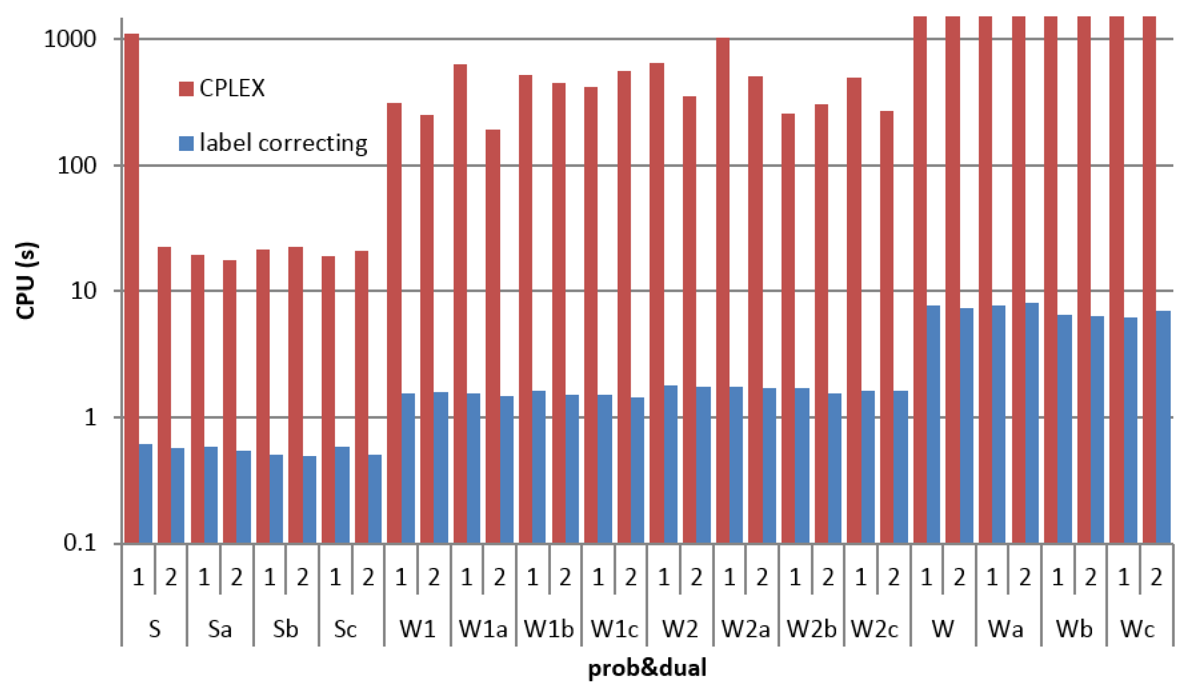
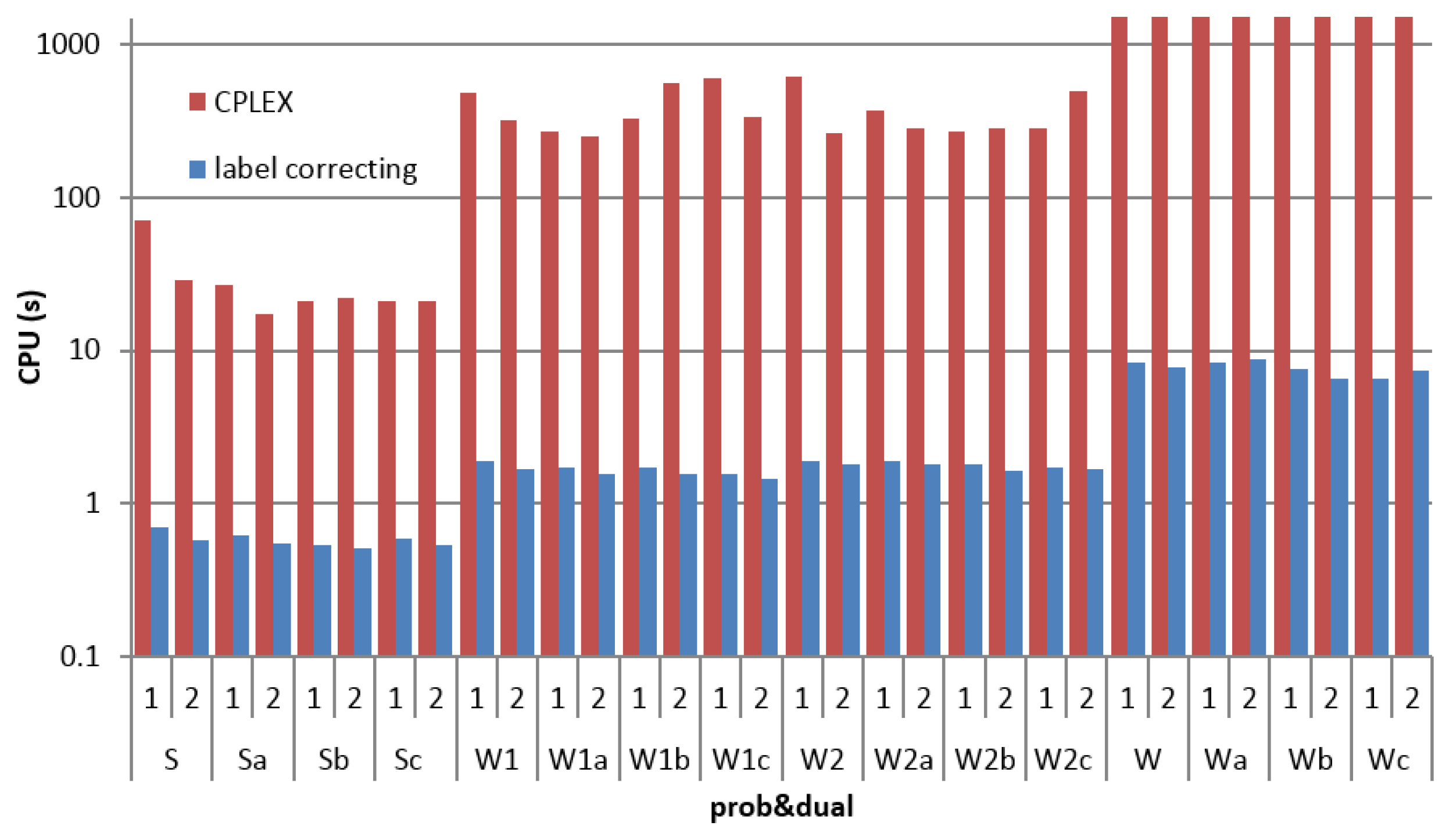
4.1. The Shortest Path in Electric Bus Scheduling with Battery Renewal

For the shortest path problem in electric bus scheduling, we used real-world data from a transit agency in the Bay Area. The transit agency is County Connection, whose data can be obtained from [44]. The data are in the GTFS (General Transit Feed Specification) format which is an open format for packaging scheduled service data. They include stop locations and published weekday and weekend schedules. The schedule includes the starting times at the stop locations. In order to conduct more tests, we divided each weekday schedule into two parts and also generated more instances by randomly shifting the trip starting time within [−10, 10] min from the original value. The ending time was also adjusted by keeping the same trip duration. Table 3 describes the problem instances. Columns 3 provides the number of time-expanded station nodes. We determined the distance between each pair of locations by solving a shortest path problem based on the real-world road geometry data provided by NavTeq. We first determined the nearest intersection to each bus stop. We then solved a one-to-one shortest path problem between each intersection using the Dijkstra algorithm. The travel times were then determined using the obtained distances and average vehicle speed of 25 mph.
The operational cost of arc (ji) is defined as: (1) if j = o, cji equals the distance cost plus the fixed vehicle maintenance cost; (2) if i S, cji equals the distance cost plus the waiting cost at i; and (3) if i T, cji equals the sum of the distance cost, the waiting cost at i and the battery service cost. The fixed vehicle maintenance cost is set as $100; the unit waiting cost is set as $0.1 per minute; and each battery service cost is set as $5. The unit distance cost is estimated based on the data from Haggis and Beback (2010) [35], which show that it can take about 8 h for a battery charger with 400 V/100 A to fully charge a battery whose operational distance is approximately 490 km. The average electricity price is set as 10.26 cents per kWh [45]. Finally, the electricity cost per kilometer is 6.61935 cents. The overall cost of arc (ji) is defined as: c ¯ ji = cji – 5 × (λi + λj), where λi and λj are dual values of nodes i and j. In order to conduct the computational experiments, we have to generate dual variables (e.g., see [14]). First, we determined the average arc operational cost by excluding the fixed vehicle cost and set it as C. Then, we generated an integer value uniformly drawn from [0.7C, 1.3C] and set it as the dual variable. In order to conduct more tests, we generated two different dual variables for each instance using different random seeds.
In accordance with real-world operations, we tested two different values of the maximum operational distance: 120 km and 150 km. We considered two different locations for the battery station. In the first case, the battery station is assumed to be located in the depot, and the computational results are shown in Table 4. In Table 4, Columns 1 and 2 provide the problem instance and dual variable ID. Columns 3 to 6 report the results when the maximum operational distance is 120 km. Column 3 provides the optimal objective value. Column 4 reports the CPU seconds of the CPLEX MIP solver. Columns 5 and 6 present the number of non-dominated labels and CPU seconds when the label-correcting algorithm is used. Columns 7 to 10 report the corresponding results when the maximum operational distance is 150 km.
In the second case, the station is assumed to be located in a bus stop that roughly centers on the overall coverage area. Figure 2 and Figure 3 show the comparison of the computational times consumed by CPLEX and label correcting for solving the problem instances for the same scenarios as in Table 4 under this case.
Table 4 and Figure 2 and Figure 3 show that the label-correcting algorithm finds the optimal solution very quickly for the instances with less than 500 trips (instances S, W1, W2 and ones that are randomly generated based on them); the computational time is less than two CPU seconds. For the large instances with 947 trips (instances W, Wa, Wb and Wc), the label-correcting algorithm spends less than 10 CPU seconds to obtain optimal solutions. The label-correcting algorithm requires much smaller computational times than CPLEX for all of the instances tested. In particular, for large instances W, Wa, Wb and Wc, CPLEX was terminated due to insufficient memory (see Columns 4 and 8 in Table 4, and the last eight red bars in Figure 2 and Figure 3). The computational time of CPLEX is larger if the maximum operational distance is smaller (for example, see Columns 4 and 8 in Table 4). In contrast, the label-correcting algorithm spends less time to obtain optimal solutions in such situations, which can be confirmed by the lesser number of non-dominated labels (see Columns 5 and 9 in Table 4). Such phenomena may be explained as follows. If the maximum operational distance is smaller, the linear programming model is more tightly constrained and is certainly more difficult for CPLEX to solve. However, in the label-correcting algorithm, the existing labels have to extend to time-expanded station nodes in T more frequently. While at time-expanded station nodes, g of all the labels is zero, and only cost c ¯ (i, g) needs to be compared in the label dominance. Therefore, the label dominance is stronger on average at time-expanded station nodes, resulting in lesser number of non-dominated labels in total. The overall computational time is then reduced.

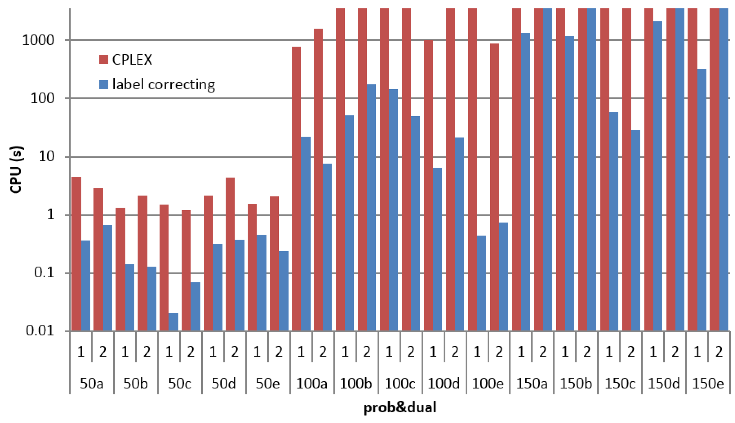
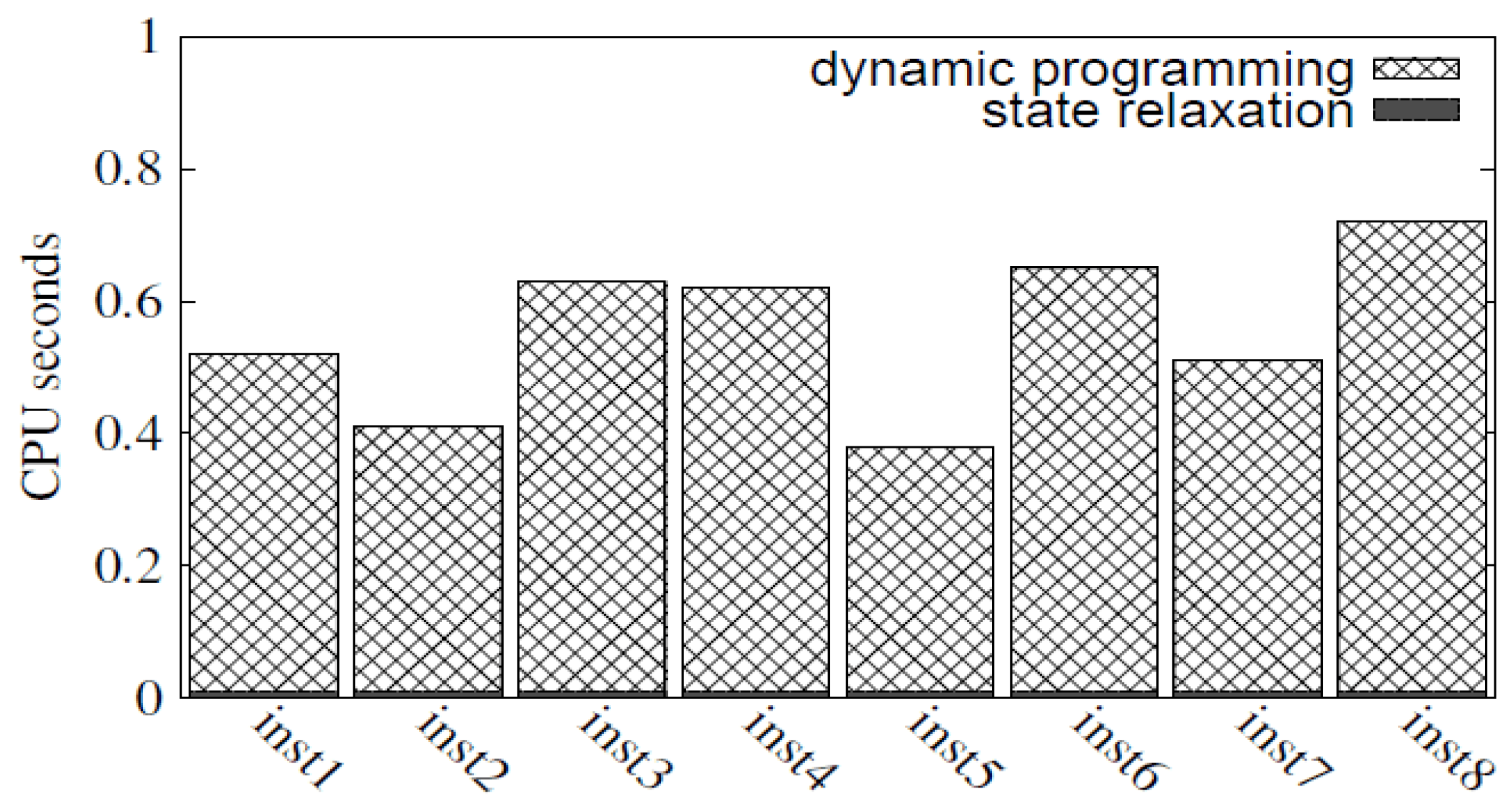
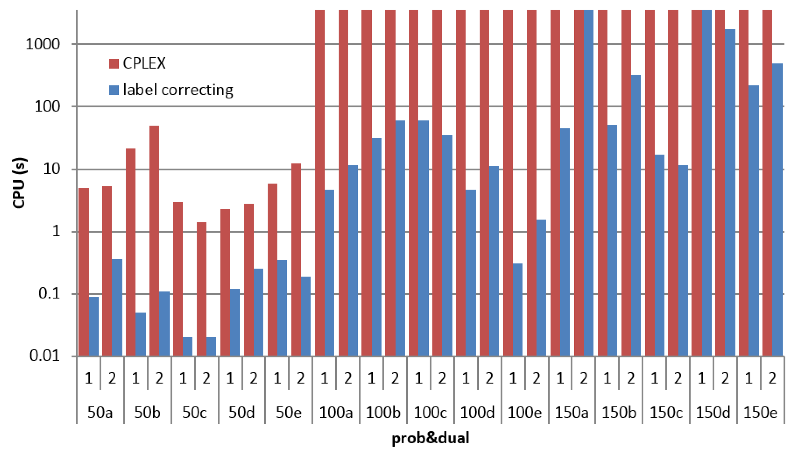
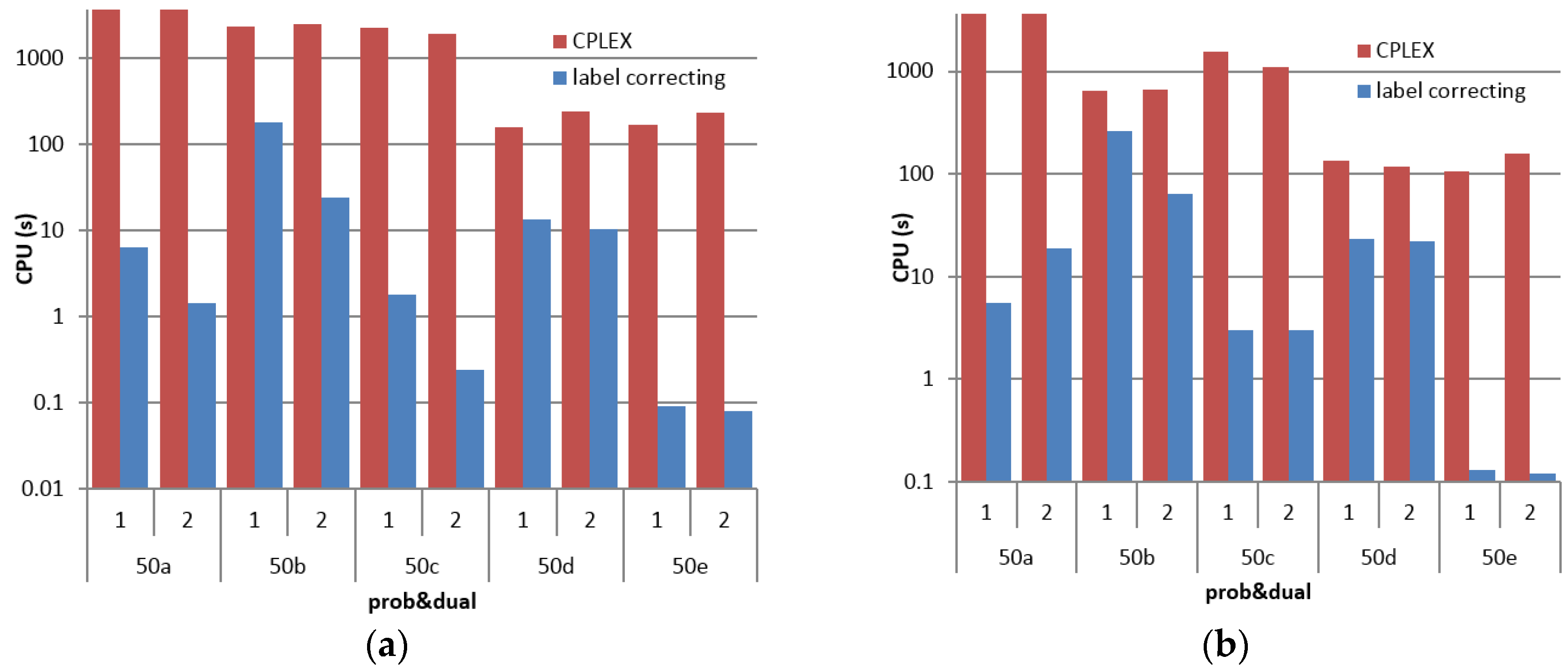
4.2. The Shortest Path in Electric Truck Routing with Battery Renewal

As discussed in Section 2.2, the current battery technique allows a truck to run about 120 to 140 km [39,40]. We tested two different values of the maximum operational distance: one was 130 km, and the other one was shorter, 100 km. In order to test the impact of the maximum operational distance in the context of real-world roads, we calculated the travel distance between two locations based on the road geometry data provided by NavTeq. We did not use the standard benchmark instances by [46]. The South Bay Area in California was selected as our case study. First, we determined | S | locations by randomly generating latitude and longitude in the South Bay Area. Then, we conducted the point-to-curve map matching to project the random location to the link in the road geometry network with the shortest perpendicular distance [47]. The point on the projected link was selected as the customer location. Finally, we solved a one-to-one shortest distance problem between each customer location using the Dijkstra algorithm based on the road geometry network. The travel times were then determined using the obtained distances and the average vehicle speed of 40 mph.
The demand at each location was randomly selected from 10, 20 and 30. The vehicle capacity was set as 400. The earliest service start time (ai) at node i S was uniformly drawn from 8 a.m. to 6 p.m. As is well known, the width of time windows has a great impact on the computational time. We tested three scenarios in terms of the width range of time windows: [5, 20] min, [5, 40] min and [5, 60] min. In each scenario, the width of time windows at each node i S was uniformly drawn from the given range. Table 5 presents the summary of generated problem instances. The operational cost of arc ji is defined as the distance cost. If i is a time-expanded station node (i.e., i T), an additional $5 is added for battery service cost. The unit distance cost was estimated based on the data from Ford Transit Connect [48], which shows that it can take about 8 h for a 6.6-kilowatt charger to fully charge a battery whose operational distance is approximately 120 km. The average electricity price was set as 10.26 cents per kWh [43]. Finally, the electricity cost per kilometer is 4.207677 cents. The overall cost of arc (ji) is defined as: c ¯ ji = cji – 5 × (λi + λj), where λi are λj generated in a similar way for electric bus scheduling.
We first briefly show the effectiveness of the state relaxation in Figure 4 with CPU seconds from eight problem instances. Figure 4 clearly shows that the state relaxation effectively reduces the computational time. From now on, we will only use the label correcting with state relaxation for further discussions. Table 6 presents the computational results for the width of time window [5, 20]. Columns 3 to 7 report the results when the maximum operational distance is 100 km. The column definitions are similar to the ones in Table 4 with the exception of Column 4, which presents the optimality gap of CPLEX, defined as|(objective value—optimal value)/objective value|, among which, the objective value is obtained from the MIP solver of CPLEX; the optimal value is from the label-correcting algorithm; and the absolute value operator is used since both values are negative. Columns 8 to 12 report the corresponding results when the maximum operational distance is 130 km.
Table 6 shows that if the width of time windows is randomly drawn from [5, 20] min, the label correcting with state relaxation finds an optimal solution within 0.2 s for the instances with 50 and 100 customers. If the number of customers is 150 or 200, the CPU seconds are in the range of [0.14, 5.51] s. The label-correcting algorithm requires much smaller computational times than CPLEX for all of the instances with the width of time windows in [5, 20]. Figure 5 shows the comparison of computational times by CPLEX and label correcting on electric truck routing with the time window width in [5, 40] min and with a maximum distance of 100 km. Figure 6 shows the corresponding comparison with a maximum distance of 130 km. Figure 7a,b shows the comparisons of computational times with the time window width in [5, 60] min, with a maximum distance of 100 km and 130 km, separately. We can find when the width of time windows is in the range [5, 40], the label-correcting algorithm still finds an optimal solution for the instances with no more than 100 customers within 3 min (see Figure 5). When the width of time windows is in [5, 60], the computational time is less than 5 min for the instances with 50 customers (see Figure 6). However, if both the number of customers and the width of time windows increase, the computational time of the label correcting often becomes substantially longer, for example instances 150a to 150e with time windows in [5, 40] in Figure 5 and Figure 6; and several instances cannot be solved by the label-correcting algorithm within one CPU hour. In comparison with the MIP solver of CPLEX, the label-correcting algorithm performs much better for most instances tested. In addition, similar to the cases in electric bus scheduling, if the maximum operational distance is smaller, the computational time of CPLEX becomes longer, while on average, the label-correcting algorithm spends less time to obtain an optimal solution. In addition, it is worthy to mention that we generated relatively large dual variables, which result in more negative cost cycles (see the objective values in Columns 3 and 8 in Table 6) and longer computational time (see Columns 5, 7, 10 and 11 in Table 6, Figure 5, Figure 6 and Figure 7).
Finally, the computational experiments show that the shortest path problem in electric truck routing is much more difficult to solve than the shortest path problem in electric bus scheduling. It takes the label-correcting algorithm less than 9 s to find the shortest paths for bus scheduling problems with 947 trips, while the label correcting may spend a much longer time to find the shortest paths for a routing instance with 100 customers and relatively wide time windows. The long computational time in electric truck routing is mainly caused by the existence of negative cost cycles in the underlying network, which leads to much more complicated label extension and dominance. The comparison of the number of non-dominated labels in electric bus scheduling and electric truck routing supports such an observation.

5. Conclusions and Future Research

In this paper, we study the shortest path problems in emerging electric vehicle dispatching, where a fully-charged battery allows a vehicle to run a limited operational distance and the battery near depletion has to be charged or exchanged with a fully-charged one at a battery management facility. The battery renewal makes the problem different from the resource-constrained shortest path problems in the literature. We investigate the shortest paths for two important applications: one is electric transit bus scheduling, and the other is electric truck routing with time windows. We develop a label-correcting algorithm to solve these shortest path problems. Since the underlying network of electric truck routing may contain negative cost cycles, the state space relaxation technique is incorporated into the label correcting to reduce the computational time.
In the computational experiments, the travel time and distance are determined based on the real-world road geometry data. Other types of data are obtained from the real-world or randomly generated. The label-correcting algorithm spends less than 9 s to find the shortest paths for electric bus scheduling problems with 947 trips. Due to the existence of negative cost cycles, the shortest path problem in electric truck routing is much more difficult to solve than in the electric bus scheduling. The label correcting with state space relaxation quickly obtains optimal solutions for the instances with 200 customers and the width of time windows in [5, 20] min. However, if both the number of customers and the width of time windows increase, the computational time often becomes substantially longer. We compare the label-correcting algorithm developed with the CPLEX MIP solver. The computational results show that the label-correcting algorithm performs much better than the CPLEX for the most instances tested, since the former is specially designed to solve the shortest path problem in electric vehicle dispatching. If the maximum operational distance is smaller, CPLEX spends a longer time for the optimal solution, while the label-correcting algorithm, on average, requires a shorter time.
The shortest path problem is a critical component in column generation algorithms since the sub-problem that is generally a shortest path problem needs to be repeatedly solved. Column generation has been successfully used in many studies to solve complicated integer programming problems [6,7]. Therefore, it is very important to develop an efficient algorithm for the shortest path problem with battery renewal. We expect that our study can play an important role in electric vehicle optimization problems.
Future work can include the development of new algorithms to reduce the computational time for instances with wide time windows. The shortest path models and algorithms can be incorporated into a column generation framework to solve electric vehicle dispatching. Investigating the location problem of battery management facilities is another topic.

Acknowledgments

This work is partially supported by the grants from the National Natural Science Foundation of China (#71201055, #71571067) and Beijing Municipal Philosophy and Social Science Planning (12JGC080).

Author Contributions

Both authors equally contributed to designing the study, analyzing the data and writing the paper.

Conflicts of Interest

The authors declare no conflict of interest.

References

  1. Environmentally Friendly Options and UPS Services. Available online: http://www.ups.com/content/us/en/bussol/browse/article/small-business-sustainability.html?srch_pos=2&srch_phr=electric+delivery+trucks (accessed on 10 December 2015).
  2. United Nations Environment Programme. UNEP Environmental Assessment Expo 2010 Shanghai, China; Tech. Rep. DCP/1209/NA; 2009. Available online: http://www.sepb.gov.cn/platform/UserFiles/File/2009-08-18-16-53-46-884+0800-570148450609847911.pdf (accessed on 23 June 2016).
  3. Beijing Electric Vehicle Promotion Application Action Plan (2014–2017). Available online: http://www.zhengwu.beijing.gov.cn/ghxx/qtgh/t1359600.htm (accessed on 12 December 2015).
  4. Desaulniers, G.; Lavigne, J.; Soumis, F. Multi-depot vehicle scheduling problems with time windows and waiting costs. Eur. J. Oper. Res. 1998, 3, 479–494. [Google Scholar] [CrossRef]
  5. Desrocher, M.; Desrosier, J.; Solomon, M.M. A new optimization algorithm for the vehicle-routing problem with time windows. Oper. Res. 1992, 2, 342–354. [Google Scholar] [CrossRef]
  6. Desrochers, M.; Soumis, F. A column generation approach to the urban transit crew scheduling problem. Transp. Sci. 1989, 1, 1–13. [Google Scholar] [CrossRef]
  7. Muter, I.; Birbil, S.I.; Bulbul, K.; Sahin, G.; Yenigun, H.; Tas, D.; Tuzun, D. Solving a robust airline crew pairing problem with column generation. Comput. Oper. Res. 2013, 3, 815–830. [Google Scholar] [CrossRef] [Green Version]
  8. Beasley, J.E.; Christo, N. An algorithm for the resource-constrained shortest-path problem. Networks 1989, 3, 379–394. [Google Scholar] [CrossRef]
  9. Desrochers, M.; Soumis, F. A generalized permanent labeling algorithm for the shortest path problem with time windows. INFOR 2014, 3, 191–212. [Google Scholar]
  10. Dumitrescu, I.; Boland, N. Improved preprocessing, labeling and scaling algorithms for the weight-constrained shortest path problem. Networks 2003, 3, 135–153. [Google Scholar] [CrossRef]
  11. Handler, G.Y.; Zang, I. A dual algorithm for the constrained shortest path problem. Networks 2006, 4, 293–309. [Google Scholar] [CrossRef]
  12. Santos, L.; Coutinho-Rodrigues, J.; Current, J.R. An improved solution algorithm for the constrained shortest path problem. Transp. Res. Part B Methodol. 2006, 7, 756–771. [Google Scholar] [CrossRef]
  13. Xing, T.; Zhou, X. Reformulation and solution algorithms for absolute and percentile robust shortest path problems. IEEE Trans. Intell. Transp. Syst. 2013, 2, 943–954. [Google Scholar] [CrossRef]
  14. Feillet, D.; Dejax, P.; Gendreau, M.; Gueguen, C. An exact algorithm for the elementary shortest path problem with resource constraints: Application to some vehicle routing problems. Networks 2004, 3, 216–229. [Google Scholar] [CrossRef]
  15. Righini, G.; Salani, M. Symmetry helps: Bounded bi-directional dynamic progrmamming for the elementary shortest path problem with resource constraints. Discret. Optim. 2006, 3, 255–273. [Google Scholar] [CrossRef]
  16. Righini, G.; Salani, M. New dynamic programming algorithms for the resource constrained elementary shortest path problem. Networks 2008, 3, 155–170. [Google Scholar] [CrossRef]
  17. Houck, D.J.; Picard, J.C.; Queyranne, M.; Vemuganti, R.R. The travelling salesman problem as a constrained shortest path problem: Theory and computational experience. Oper. Res. 1980, 2, 93–109. [Google Scholar]
  18. Irnich, S.; Villeneuve, D. The shortest-path problem with resource constraints and k-cycle elimination for k > 3. INFORMS J. Comput. 2006, 3, 391–406. [Google Scholar] [CrossRef]
  19. Bode, C.; Irnich, S. The shortest-path problem with resource constraints with (k, 2)-loop elimination and its application to the capacitated arc-routing problem. Eur. J. Oper. Res. 2014, 2, 415–426. [Google Scholar] [CrossRef]
  20. Garey, M.R.; Johnson, D.S. Computers and Intractability: A Guide to the Theory of NP-Completeness, 1st ed.; W.H. Freeman: New York, NY, USA, 1979. [Google Scholar]
  21. Wang, Y.W.; Lin, C.C. Locating road-vehicle refueling stations. Transp. Res. Part E Logist. Transp. Rev. 2009, 5, 821–829. [Google Scholar] [CrossRef]
  22. Yildiz, B.; Arslan, O.; Karasan, O.E. A branch and price approach for routing and refueling station location model. Eur. J. Oper. Res. 2015, 3, 815–826. [Google Scholar]
  23. Huang, S.; He, L.; Gu, Y.; Wood, K.; Benjaafar, S. Design of a mobile charging service for electric vehicles in an urban environment. IEEE Trans. Intell. Transp. Syst. 2014, 2, 787–798. [Google Scholar] [CrossRef]
  24. Kang, Q.; Wang, J.; Zhou, M.; Ammari, A.C. Centralized charging strategy and scheduling algorithm for electric vehicles under a battery swapping scenario. IEEE Trans. Intell. Transp. Syst. 2015, 1, 1–11. [Google Scholar] [CrossRef]
  25. Roberti, R.; Wen, M. The electric traveling salesman problem with time windows. Transp. Res. Part E Logist. Transp. Rev. 2016, 89, 32–52. [Google Scholar] [CrossRef] [Green Version]
  26. Bruglieri, M.; Pezzella, F.; Pisacane, O.; Suraci, S. A variable neighborhood search branching for the electric vehicle routing problem with time windows. Electron. Notes Discret. Math. 2015, 47, 221–228. [Google Scholar] [CrossRef]
  27. Yang, J.; Sun, H. Battery swap station location-routing problem with capacitated electric vehicles. Comput. Oper. Res. 2015, 55, 217–232. [Google Scholar] [CrossRef]
  28. Yagcitekin, B.; Uzunoglu, M. A double-layer smart charging strategy of electric vehicles taking routing and charge scheduling into account. Appl. Energy 2016, 167, 407–419. [Google Scholar] [CrossRef]
  29. Elkins, J.; Hemby, J.; Rao, V.; Szykman, J.; Fitz-Simons, T.; Doll, D.; Mintz, D.; Rush, A.; Frank, N.; Schmidt, M.; et al. National Air Quality and Emission Trends Report Special Studies Edition; U.S. Environmental Protection Agency: North Carolina, CA, USA, 2003.
  30. O’brien, W.A. Electric vehicles (EVs): A look behind the scenes. IEEE Aerosp. Electron. Syst. Mag. 1993, 5, 38–41. [Google Scholar] [CrossRef]
  31. Argonne National Laboratory. Electric Buses Energize Downtown Chattanooga. Available online: http://www.afdc.energy.gov/afdc/pdfs/chatt_cs.pdf (accessed on 12 December 2015).
  32. Beijing Readies Electric Buses for Summer Olympics. Available online: http://www.evworld.com/news.cfm?newsid=18730 (accessed on 13 December 2015).
  33. Namsan Electric Bus Cruises into International Limelight. Available online: http://www.cnngo.com/seoul/life/namsan-electric-bus-cruises-limelight-262862 (accessed on 13 December 2015).
  34. Quick-charge Electric Bus Rolls into L.A. County. Available online: http://www.wired.com/autopia/2010/09/proterra-ecoride-foothill-transit (accessed on 13 December 2015).
  35. Transi. Bus Technology Feasibility Study. Available online: http://www.advancedenergy.org/transportation/additional_efforts/TransitBusFeasibilityStudy_Final.pdf (accessed on 20 December 2015).
  36. Final Environmental Review of the 2010 World Exposition. Available online: http://www.unep.org/newscentre/Default.aspx?DocumentID=2659&ArticleID=8964&l=en#sthash.zr7SV1wK.dpuf (accessed on 15 November 2015).
  37. Shafia, M.A.; Aghaee, M.P.; Sadjadi, S.J.; Jamili, A. Robust train timetabling problem: Mathematical model and branch and bound algorithm. IEEE Trans. Intell. Transp. Syst. 2012, 1, 307–317. [Google Scholar] [CrossRef]
  38. Li, J.Q. Transit bus scheduling with limited energy. Transp. Sci. 2013, 4, 521–539. [Google Scholar] [CrossRef]
  39. UPS’ Brown Trucks Get Greener with Electric Power. Available online: http://www.sfgate.com/cgi-bin/article.cgi?f=/c/a/2011/08/25/BU7I1KRF10.DTL (accessed on 12 December 2015).
  40. Ford Transit Connect Electric Commercial van Helps Customers Go Completely Gas-Free. Available online: http://www.media.ford.com/article_display.cfm?article_id=31991 (accessed on 12 December 2015).
  41. Boland, N.; Dethridge, J.; Dumitrescu, I. Accelerated label setting algorithms for the elementary resource-constrained shortest path problem. Oper. Res. Lett. 2004, 1, 58–68. [Google Scholar] [CrossRef]
  42. Christo, N.; Mingozzi, A.; Toth, P. State-space relaxation procedures for the computation of bounds to routing problems. Networks 2006, 2, 145–164. [Google Scholar]
  43. IBM Cplex. Available online: https://www-01.ibm.com/software/commerce/optimization/cplex-optimizer/ (accessed on 9 June 2016).
  44. GTFS data. Available online: http://www.gtfs-data-exchange.com/agency/county-connection (accessed on 12 December 2015).
  45. Energy Information Administration. (2011, Dec). Prices and Factors Affecting Prices. Available online: http://www.eia.gov/energyexplained/index.cfm?page=electricity_factors_affecting_prices (accessed on 12 December 2015).
  46. Solomon, M.M. Algorithms for the vehicle-routing and scheduling problems with time window constraints. Oper. Res. 1987, 2, 254–265. [Google Scholar] [CrossRef]
  47. Li, J.Q. Match bus stops to a digital road network by the shortest path model. Transp. Res. Part C Emerg. Technol. 2012, 2, 119–131. [Google Scholar] [CrossRef]
  48. Ford Working with Best Buy to Offer Focus Electric Charging Station Sales, Installation and Support. Available online: http://www.media.ford.com/article_display.cfm?article_id=33772 (accessed on 12 December 2015).
Figure 1. The flowchart of the label-correcting algorithm.
Sustainability 08 00607 g001
Figure 2. The computational times by CPLEX and label correcting on scheduling with a maximum distance of 120 km and the battery station centering on the service area.
Sustainability 08 00607 g002
Figure 3. The computational times by CPLEX and label correcting on scheduling with a maximum distance of 150 km and the battery station centering on the service area.
Sustainability 08 00607 g003
Figure 4. The performance of the dynamic programming with state relaxation.
Sustainability 08 00607 g004
Figure 5. The computational times by CPLEX and label correcting on electric truck routing with the time window width in [5, 40] min and a maximum distance of 100 km.
Sustainability 08 00607 g005
Figure 6. The computational times by CPLEX and label correcting on electric truck routing with the time window width in [5, 40] min and a maximum distance of 130 km.
Sustainability 08 00607 g006
Figure 7. The computational times by CPLEX and label correcting on electric truck routing with the time window width in [5, 60] min. (a) with a maximum distance of 100 km; (b) with a maximum distance of 130 km.
Sustainability 08 00607 g007
Table 1. The mathematical model of the shortest path problem in electric transit bus scheduling with battery renewal.
Objective Function and RestrictionsVariable RangeEquation No.
min ( j , i ) ϵ A c ¯ j i x j i (a1)
st
j : ( i , j ) ϵ A x i j = 1 i = o (a2)
j : ( j , i ) ϵ A x j i = 1 i = d (a3)
i : ( j , i ) ϵ A x j i i : ( i , j ) ϵ A x i j = 0 j S T (a4)
g i = j : ( j , i ) ϵ A ( g j + d j i ) x j i i S (a5)
g i = 0 i T { o } (a6)
( g j + d j t ) x j t     D t T { d } , ( j , t ) A (a7)
x i j { 0 , 1 } ( i , j ) A
Table 2. The mathematical model of the shortest path problem in electric truck routing with the time windows.
Objective Function and RestrictionsVariable RangeEquation No.
min ( j , i ) ϵ A c ¯ j i x j i (b1)
st
(a2) − (a7) (b2)
s j + U j + t j i     s i + M ( 1   x j i ) ( j , i ) A , i S T (b3)
a i s i b i i S (b4)
s 0 = 0 (b5)
( j , i ) ϵ A v i x j i V (b6)
x i j { 0 , 1 } ( i , j ) A (b7)
Table 3. Description of instances in electric bus scheduling.
Instance# of Trips# of Time-Expanded NodesDescription
S
Sa
Sb
Sc
242952
951
943
930
published weekend schedules
randomly-generated based S
same as above
same as above
W
Wa
Wb
Wc
9471132
1136
1136
1130
published weekday schedules
randomly-generated based W
same as above
same as above
W1
W1a
W1b
W1c
4631073
1087
1074
1084
half of W
randomly-generated based W1
same as above
same as above
W2
W2a
W2b
W2c
4841132
1131
1124
1126
the other half of W
randomly-generated based W2
same as above
same as above
Table 4. Results on scheduling with the battery station in the depot.
InstanceDualMax Distance 120 kmMax Distance 150 km
Optimal Objective ValueCPLEXLabel CorrectingOptimal Objective ValueCPLEXLabel Correcting
CPU (s)LabelsCPU (s)CPU (s)LabelsCPU (s)
S
 
Sa
 
Sb
 
Sc
 
1
2
1
2
1
2
1
2
–822,351
–819,804
–707,440
–705,225
–712,234
–724,879
–751,972
–790,796
117.94
1167.49
26.77
39.38
45.25
26.09
101.99
33.72
2875
2668
1735
2065
1917
2134
2305
2283
0.72
0.72
0.53
0.52
0.54
0.54
0.57
0.56
–824,405
–829,648
–707,440
–705,225
–712,234
–724,879
–755,469
–790,796
141.92
61.65
27.79
32.6
38.13
29.23
42.92
40.46
2897
2739
1735
2066
1919
2134
2511
2302
0.74
0.78
0.55
0.58
0.56
0.6
0.6
0.58
W1
 
W1a
 
W1b
 
W1c
 
1
2
1
2
1
2
1
2
–1,175,252
–1,185,467
–1,190,403
–1,140,363
–1,180,257
–1,133,505
–1,226,202
–1,160,532
2927.46
338.88
262.11
328.97
738.82
249.87
248.59
+
3239
3012
3123
3075
3431
2702
3116
4126
1.64
1.62
1.5
1.46
1.46
1.35
1.69
1.53
–1,175,252
–1,185,467
–1,190,403
–1,140,363
–1,181,390
–1,133,505
–1,226,202
–1,162,385
+
273.81
273.04
256.57
298.17
808.2
251.33
1052.89
3287
2987
3123
3078
3639
2717
3118
4513
1.74
1.71
1.58
1.56
1.69
1.41
1.8
1.65
W2
 
W2a
 
W2b
 
W2c
 
1
2
1
2
1
2
1
2
–1,241,010
–1,250,571
–1,236,314
–1,293,550
–1,271,817
–1,228,527
–1,321,741
–1,279,684
1142.48
339.46
314.43
421.19
3565.16
1645.09
376.29
274.28
3060
3133
3492
2899
4166
3831
3967
3681
1.69
1.65
1.61
1.62
1.53
1.56
1.81
1.84
–1,241,010
–1,250,571
–1236,314
–1293,550
–1286,476
–1235,273
–1,321,741
–1,279,684
+
593.26
481.85
1513.48
505.13
424.58
362.13
311.64
3195
3205
3548
2924
4906
4133
3990
3742
1.82
1.74
1.66
1.68
1.58
1.67
1.92
1.97
W
 
Wa
 
Wb
 
Wc
 
1
2
1
2
1
2
1
2
–1,614,504
–1,574,276
–1,465,572
–1,513,933
–1,484,716
–1,469,219
–1,490,073
–1,518,417
*
*
*
*
*
*
*
*
8333
7751
7953
8779
13,329
8644
8952
12,600
8.58
8.13
7.47
8.04
8.24
7.99
8.04
8.72
–1,628,219
–1,590,012
–1,471,389
–1,518,442
–1,495,817
–1,502,780
–1,498,017
–1,526,627
*
*
*
*
*
*
*
*
9104
8420
8228
9101
16,182
10,332
10,500
14,393
9.65
8.96
8.21
9.07
9.42
8.74
9.36
9.74
* CPLEX was terminated due to being out of memory; +: no an optimal solution was found within 1 CPU hour.
Table 5. Description of the instances in electric truck routing.
Instance# of Customers# of Time-Expanded NodesInstance# of Customers# of Time-Expanded Nodes
Time WindowsTime Windows
[5, 20] min[5, 40] min[5, 60] min[5, 20] min[5, 40] min
50a50620665685150a150662695
50b50585666687150b150636677
50c50623661681150c150652716
50d50597641665150d150638696
50e50547644653150e150665686
100a100644656662200a200667678
100b100634639663200b200664680
100c100655693696200c200633680
100d100645680700200d200645660
100e100658683697200e200656694
Table 6. Results on electric truck routing with the time window width in [5, 20] min.
InstanceDualMax Distance 100 kmMax Distance 130 km
Optimal Objective ValueCPLEXState RelaxationOptimal Objective ValueCPLEXState Relaxation
Optimal GapCPU (s)LabelsCPU (s)Optimal GapCPU (s)LabelsCPU (s)
50a1−62200.000.6317440.02−62200.000.7017800.02
2−53140.000.6314910.02−53140.000.6115390.02
50b1−87420.000.5728960.01−87420.000.5729040.01
2−83200.000.5532040.02−83200.000.5732080.02
50c1−71950.000.5026570.01−71950.000.5027710.02
2−74870.000.5326290.01−74870.000.4928240.01
50d1−12,2340.000.5434120.02−12,2340.000.5438460.02
2−11,8070.000.5944050.02−11,8070.000.56 48410.02
50e1−79860.000.4721630.01−79860.000.4924040.01
2−79620.000.4822870.01−79620.000.4525360.01
100a1−11,7730.001.6650880.04−11,7730.001.4554830.04
2−12,3850.001.3753640.05−12,3850.001.3557540.04
100b1−12,2920.003.8490080.09−13,1950.001.5595880.1
2−10,7740.005.4196150.10−11,4940.001.5910,2770.11
100c1−11,6550.001.2762110.05−11,6550.001.2364460.06
2−90250.001.3352530.04−90250.001.3855390.04
100d1−13,4050.001.7095430.08−13,4050.001.55 98160.09
2−12,5760.001.5310,1920.10−12,5760.001.6710,3910.1
100e1−13,4730.001.6110,5460.10−13,4730.001.5011,2080.11
2−14,9370.001.5781340.08−14,9370.001.5386280.08
150a1−14,9800.004.9920,9420.84−16,1590.003.4821,5480.84
2−16,3270.006.8018,0390.75−16,8830.004.6618,7260.75
150b1−15,4930.004.5612,5880.14−15,4930.004.5412,9130.15
2−14,0260.006.8599660.13−14,0260.005.8610,1670.14
150c1−17,0620.003.1814,0510.62−17,0620.005.2414,1180.65
2−16,2920.004.1318,6261.50−16,2920.004.3218,7381.58
150d1−18,1580.0010.7029,8283.36−19,6560.004.6131,4412.34
2−17,7440.0012.9019,9411.48−18,5870.005.9926,2331.87
150e1−17,9250.0043.7123,9110.42−19,2140.0011.7026,7440.44
2−19,3970.0024.2923,2810.38−21,2700.006.9625,4910.39
200a1−17,7180.0015.9325,2002.40−19,2650.0013.0924,3900.53
2−18,8910.0024.2830,5532.68−18,8910.0010.1426,2012.37
200b1−21,3000.0013.0726,9690.53−22,2160.007.1827,0310.54
2−22,3000.0012.2120,3030.36−23,1120.006.9520,3960.38
200c1−18,3360.0014.0023,5121.29−19,2600.006.1925,3161.43
2−17,1940.0014.9025,7442.46−18,2120.006.5426,9672.46
200d1−19,5360.0027.9246,0374.80−20,7420.0067.1648,7684.93
2−20,3150.0092.3746,0882.80−20,6070.0058.9746,3425.51
200e1−20,5410.0014.9230,2010.62−20,5410.0018.2130,8080.65
2−21,1710.0036.2820,9171.00−22,3030.0021.4721,4130.98

