Optimization Model for Mitigating Global Warming at the Farm Scale: An Application to Japanese Rice Farms

Abstract

In Japan, greenhouse gas emissions from rice production, especially CH₄ emissions in rice paddy fields, are the primary contributors to global warming from agriculture. When prolonged midseason drainage for mitigating CH₄ emissions from rice paddy fields is practiced with environmentally friendly rice production based on reduced use of synthetic pesticides and chemical fertilizers, Japanese rice farmers can receive an agri-environmental direct payment. This paper examines the economic and environmental effects of the agri-environmental direct payment on the adoption of a measure to mitigate global warming in Japanese rice farms using a combined application of linear programming and life cycle assessment at the farm scale. Eco-efficiency, which is defined as net farm income divided by global warming potential, is used as an integrated indicator for assessing the economic and environmental feasibilities. The results show that under the current direct payment level, the prolonged midseason drainage technique does not improve the eco-efficiency of Japanese rice farms because the practice of this technique in environmentally friendly rice production causes large economic disadvantages in exchange for small environmental advantages. The direct payment rates for agri-environmental measures should be determined based on the condition that environmentally friendly agricultural practices improve eco-efficiency compared with conventional agriculture.

1. Introduction

Agri-environmental payments are one of the few politically sustainable forms of government support to agriculture [1]. They encourage management practices that benefit the environment, and provide economic incentives for the adoption of eco-efficient systems to farmers [2,3]. In European countries, since the 1980s, the management of landscapes, biodiversity, natural resources, the soil, and genetic diversity have been supported by agri-environment schemes [2]. In Japan, although agri-environmental payments have primarily been used to improve water pollution, they have recently been used for global warming mitigation as part of the environmental targets [4,5].

The increased atmospheric concentrations of greenhouse gases (GHGs) caused by human activities have contributed to global warming [6]. In agricultural production, fossil fuel combustion, enteric fermentation, manure management, flooded paddy fields, nitrogen inputs in the soil, etc., are emission sources of CO₂, CH₄, and N₂O [7]. Of these GHGs, CH₄ has a greater impact on global warming than CO₂ and is the second largest driver of radiative forcing, which is a measure of the net change in the energy balance of the Earth system in response to some external perturbation [6]. One of the dominant anthropogenic sources of CH₄ is rice cultivation [6]. In Asian countries, where rice is a staple food, CH₄ emissions from rice paddy fields are a significant component of total GHG emissions from agriculture [8]. In Japan, CH₄ emitted from rice paddy fields is the third largest contributor (23%) to global warming from the agricultural sector [7], and, thus, its reduction will mitigate GHG emissions from agriculture.

There are several effective strategies for reducing CH₄ emissions from rice paddy fields, such as altering water management, applying soil amendments, and improving organic matter management [9]. Of these, prolonged midseason drainage, which is supported by the Japanese agri-environmental payment program, is one of several simple and feasible management strategies for mitigating CH₄ emissions from rice paddy fields [4,10]. However, because both reductions of CH₄ emissions and rice yields come from prolonging midseason drainage [9,10], both the environmental and economic feasibility should be considered when assessing this technique.

To determine the trade-off between the economic and environmental feasibilities of adopting environmental measures and/or evaluate the economic and environmental impacts of policy changes, previous studies have applied optimization models at the farm scale to rice farms [11,12], arable farms [13,14], arable and livestock farms [15,16], and dairy farms [17,18,19,20]. Of these, Glithero et al. [13], Nakashima [14], and Van Calker et al. [19] evaluated GHG emissions as an ecological indicator; however, their analyses did not include rice paddy fields, which are an important source of CH₄ emissions. On the other hand, in Chono et al. [11] and Senthilkumar et al. [12], only nitrogen was taken into account as a pollutant emitted from rice paddy fields. Consequently, previous studies have not addressed the problems of adopting mitigation measures to global warming in rice farms.

This paper examines the economic and environmental effects of agri-environmental direct payments on mitigating global warming in Japanese rice farms. Three primary GHGs (CO₂, CH₄, and N₂O) emitted from Japanese rice farms, which might cultivate not only rice but also wheat and soybeans under the rice production adjustment program [21], were taken into account as contributing to global warming. A prolonged midseason drainage technique was selected as a measure to mitigate global warming, because it primarily reduces CH₄ emissions in rice paddy fields. The economic, environmental, and integrated feasibilities of prolonging midseason drainage are assessed using net farm income, global warming impact, and eco-efficiency (net farm income per unit of global warming impact), respectively.

Two research questions are addressed in the paper. The first is whether Japanese rice farms have some advantages in producing environmentally friendly rice under the current conditions. The second is how Japanese rice farms are affected when the direct payment for environmentally friendly rice production is increased gradually.

The paper is structured as follows. Section 2 describes the materials and methods for building an optimization model and assessing GHG emissions. Section 3 presents the results of net farm income, global warming impact, and eco-efficiency, followed by discussion in Section 4 of our findings in relation to the two research questions. Section 5 provides concluding remarks.

2. Materials and Methods

2.1. Agri-Environmental Direct Payment Program in Japan

The direct payment program for environmentally friendly agriculture in Japan, which was started in 2011, aims to support farming practices for global warming mitigation and biodiversity conservation [4]. Supported farmers can receive 30,000–80,000 yen per ha when they select any one of cover cropping, manure application, or local special practices with crop production based on reduced use of synthetic pesticides and chemical fertilizers, and use of organic agriculture [4,22]. They primarily cultivate crops based on reduced use of synthetic pesticides and chemical fertilizers, defined as reductions in the frequency of synthetic pesticide application and in chemical nitrogen fertilizer inputs to less than 50% of the levels seen in conventional agriculture [4]. The supported land area for the practices associated with reduced use of synthetic pesticides and chemical fertilizers covers 74% of the total area (51,114 ha) supported by this program [23].

In the Shiga region, which is located near Kyoto and includes Lake Biwa, the largest lake in Japan, the prefecture’s direct payment subsidies for environmentally friendly agriculture based on reduced use of synthetic pesticides and chemical fertilizers have been paid to farmers since 2004, which is earlier than for the rest of Japan [5]. The Shiga region has the largest supported area (8639 ha) for the practices associated with reduced use of synthetic pesticides and chemical fertilizers in the present program [23], of which approximately 90% is used for rice production [24]. The local special practice with reduced use of synthetic pesticides and chemical fertilizers that includes integrated pest management, mechanical weeding at paddy field dikes, and prolonged midseason drainage with cutting furrows covers 7049 ha [24], and its direct payment per hectare is 40,000 yen [22]. In this paper, this practice was selected as a prolonged midseason drainage technique to be assessed.

2.2. Farm Modeling

Previous studies have undertaken farm modeling based on combination of existing literature [11,13,14,17,18,19], existing models [15,16,20], or farm surveys [12]. In this paper, a combination of existing literature, especially farm management handbooks, was used for farm modeling [14]. Data on crop production activities, land use activities, and labor inputs were collected as fundamental information required for farm modeling [13,14,17,18,19].

Table 1. Overview of the modeled farm ¹.

Item	Characteristics
Farmland area	27 ha (1 ha privately owned; 26 ha leased)
Planted crops	CR or EFR (VEV, EV, MV, and LV) CW (MV) and CS (MV and LV) under the rice production adjustment program
Cropping patterns	Continuous rice cultivation every year Rice–wheat–soybean rotation every two years
Labor force	Two family members Minimum number of temporary workers for mechanical weeding at paddy field dikes in early June, early July, late July, mid-August, and late September
Entrusted operations	Chemical control of pests and diseases in CR production Chemical pest control in EFR production Chemical disease control in CW production Grain drying in CW and CS production

CR = conventional rice, EFR = environmentally friendly rice, CW = conventional wheat, CS = conventional soybeans, VEV = very early variety, EV = early variety, MV = medium variety, and LV = late variety; ¹ The modeled farm was built using the farm management handbook [21] and modified after personal communication with Shiga Prefecture [24]. Because the cultivation protocols for conventional rice were not included in Shiga Prefecture [21], they were developed by modifying those of environmentally friendly rice by reference to the old protocols [25].

presents an overview of the modeled farm. To generate enough net farm income, the modeled farm had 27 ha. The planted crops were rice produced conventionally or using environmentally friendly principles and wheat and soybeans produced conventionally under the rice production adjustment program. Continuous rice cultivation and a two-year rice–wheat–soybean rotation were taken into account in the cropping patterns. The labor force was comprised of two family members in addition to the minimum number of temporary workers for mechanical weeding at paddy field dikes to avoid labor shortages. Although most agricultural operations in the modeled farm were performed by family and temporary workers, several operations were entrusted to agricultural contractors. When addressing the two research questions dealt with in this paper, comparisons were made between the modeled farm with conventional rice production (CR farm) and the modeled farm with environmentally friendly rice production (EFR farm).

As noted, environmentally friendly rice production with reduced use of synthetic pesticides and chemical fertilizers was based on the local special practice including integrated pest management, mechanical weeding at paddy field dikes, and prolonged midseason drainage with cutting furrows. There were differences in pesticide application, fertilizer use, and water management between conventional and environmentally friendly rice production (

Table 2. Differences in operations between conventional and environmentally friendly rice production ¹.

	CR	EFR
Pesticide application	Chemical seed disinfection Fungicide injection into nursery soil at seeding Herbicide application soon after transplanting Two chemical pest and disease control treatments	Hot water disinfection for seeds Use of fungicide and insecticide mixtures in nursery boxes Herbicide application at the time of transplanting One chemical pest control treatment
Fertilization	Chemical fertilizers Soil amendments	Organic-inorganic compound fertilizers Soil amendments
Period of midseason drainage 2	7 days	14 days

CR = conventional rice and EFR = environmentally friendly rice; ¹ [21,22,25,26]; ² Labor inputs for prolonged midseason drainage were deemed the same as those for conventional midseason drainage because differences between them in water management operations such as patrols for water monitoring were very small [22,26].

). Prolonged midseason drainage performed in environmentally friendly rice production contributes to mitigating CH₄ emissions in paddy fields, which occur under anaerobic conditions by the action of microbes [7,10].

2.3. Linear Programming Model

The farm-scale optimization model used in this paper has the form of a standard linear programming model. When farmers behave to maximize net farm income under the constraints for land use activities and labor inputs, the problem for the modeled farm is expressed as

$$\mathrm{maximize} NFI={\displaystyle \sum _{i=1}^{11}{a}_i{x}_i-0.001{\displaystyle \sum _{j=1}^5{y}_j-16.56}}$$

(1)

subject to

$$27\ge {\displaystyle \sum _{i=1}^9{x}_i}$$

(2)

$$27\ge {\displaystyle \sum _{i=1}^8{x}_i}+{\displaystyle \sum _{i=10}^{11}{x}_i}$$

(3)

$$0\ge -{\displaystyle \sum _{i=1}^8{x}_i}+x_9$$

(4)

$$0\ge -x_9+{\displaystyle \sum _{i=10}^{11}{x}_i}$$

(5)

$$0\ge -0.7x_9+x_{10}$$

(6)

$$0\ge 0.33{\displaystyle \sum _{i=1}^8{x}_i}-0.67x_9$$

(7)

$$h_k\ge {\displaystyle \sum _{i=1}^{11}{b}_{ik}{x}_i}-z_k\left(k=1,\mathrm{...},36,z_k=\{\begin{array}{ll}{y}_1& \text{if the term is early June},\\ y_2& \text{if the term is early July},\\ y_3& \text{if the term is late July},\\ y_4& \text{if the term is mid-August},\\ y_5& \text{if the term is late September},\\ 0& \text{otherwise}\end{array}\right)$$

(8)

$$79\ge {\displaystyle \sum _{j=1}^5{y}_j}$$

(9)

$$0\ge -5{\displaystyle \sum _{i=1}^9{x}_i+y_1}$$

(10)

$$0\ge -5{\displaystyle \sum _{i=1}^8{x}_i+y_2}$$

(11)

$$0\ge -5\left({\displaystyle \sum _{i=1}^8{x}_i}+{\displaystyle \sum _{i=10}^{11}{x}_i}\right)+y_3$$

(12)

$$0\ge -5{\displaystyle \sum _{i=1}^8{x}_i+y_4}$$

(13)

$$0\ge -5{\displaystyle \sum _{i=10}^{11}{x}_i}+y_5$$

(14)

$$x_i\ge 0,\forall i$$

(15)

$$y_j\ge 0,\forall j$$

(16)

where NFI is the net farm income (million yen); a_i is the ith crop income (million yen per ha); x_i is the ith crop-planted area (ha); y_j is the jth input of temporary workers (hours); h_k is the family labor input in the kth term (hours); b_ik is the labor input required for the ith crop in the kth term (hours per ha); and z_k is the input of temporary workers in the kth term (hours). The subscript i refers to planted crops: very early-, early-, medium-, and late-maturing rice varieties produced conventionally (i = 1, 2, 3, 4, respectively); very early-, early-, medium-, and late-maturing rice varieties produced on environmentally friendly principles (i = 5, 6, 7, 8, respectively); a medium-maturing wheat variety produced conventionally (i = 9); and medium- and late-maturing soybean varieties produced conventionally (i = 10, 11, respectively). In the subscript j, the inputs of temporary workers in early June, early July, late July, mid-August, and late September are numbered, respectively, from one to five. Because every month was divided into three (early, middle, late) terms, Equation (8) is comprised of 36 functions (k = 1, …, 36).

To calculate net farm income in Equation (1), the payments to temporary workers, fixed and common costs, and deduction of the direct payment for rice production are subtracted from the total crop income. The crop income coefficients (a_i) are shown in

Table 3. Yields and crop income coefficients (t per ha; million yen per ha).

	CR				EFR				CW	CS
	VEV	EV	MV	LV	VEV	EV	MV	LV	MV	MV	LV
Yield 1	5.1	5.4	5.7	5.1	4.6	4.9	5.2	4.6	3.6	2.0	2.0
Gross income 2	0.95	1.10	1.07	0.95	0.92	1.06	1.04	0.92	0.04	0.18	0.18
Subsidy 3	0.075	0.075	0.075	0.075	0.115	0.115	0.115	0.115	0.796	0.539	0.539
Production cost 4	0.31	0.32	0.31	0.31	0.37	0.37	0.37	0.36	0.32	0.27	0.27
Crop income 5	0.71	0.86	0.84	0.72	0.67	0.81	0.79	0.67	0.52	0.44	0.44

CR = conventional rice, EFR = environmentally friendly rice, CW = conventional wheat, CS = conventional soybeans, VEV = very early variety, EV = early variety, MV = medium variety, and LV = late variety; ¹ It was assumed that the yields of conventional rice with normal midseason drainage were 106.0% [28] and yields of environmentally friendly rice with prolonged midseason drainage were 96.2% [10] of those of environmentally friendly rice with normal midseason drainage [21]. Conventional wheat and soybean yields were derived from Shiga Prefecture [21]; ² Gross income for each crop was calculated by multiplying the yield by the unit price. The unit prices for conventional rice, environmentally friendly rice, conventional wheat, and conventional soybeans were 188–203, 200–217, 12.2, and 87.8–88.7 yen per kg, respectively [21,28]; ³ The income stabilization program for farmers and the direct payment program for environmentally friendly agriculture were taken into account in the subsidies [22,24,27]; ⁴ [21,25,29]; ⁵ Crop income = Gross income + Subsidy − Production cost.

. The hourly wage of temporary workers as the coefficient of y_j was 1000 yen [21]. The fixed and common costs and deduction of the direct payment for rice production were 16.55 million yen [21] and 7500 yen [27], respectively.

Equations (2)–(7) indicate the constraints for land use activities. Because the growing season of rice (April–September) overlaps with that of either wheat (October–June) or soybeans (June–November), the total planted area of rice and wheat or soybeans is 27 ha or less (Equations (2) and (3)) [21]. The cropping patterns adopted are continuous rice cultivation and/or a two-year rice–wheat–soybean rotation. When a two-year rice–wheat–soybean rotation is selected, wheat is planted after harvesting rice, and soybeans are cultivated following wheat harvesting [21]. Thus, the wheat-planted area cannot exceed the rice-planted area (Equation (4)), and the soybean-planted area cannot exceed the wheat-planted area (Equation (5)). However, a medium-maturing soybean variety can be planted in up to 70% of wheat-cultivated land, which is harvested in mid-June when the first field operation (soil amendment application) for a medium-maturing soybean variety is performed (Equation (6)) [21]. The planted area for rice cannot exceed two-thirds of total farmland because of the rice production adjustment program (Equation (7)) [21].

Equations (8)–(14) represent the constraints for labor inputs.

Table 4. Labor input coefficients (hours per ha) ¹.

		CR				EFR				CW	CS
		VEV	EV	MV	LV	VEV	EV	MV	LV	MV	MV	LV
January	Early	0	0	0	0	0	0	0	0	1.6	0	0
	Middle	0	0	0	0	0	0	0	0	0	0	0
	Late	0	0	0	0	0	0	0	0	0	0	0
February	Early	0	0	0	0	0	0	0	0	0	0	0
	Middle	0	0	0	0	0	0	0	0	0	0	0
	Late	0	0	0	0	0	0	0	0	0	0	0
March	Early	0	0	0	0	0	0	0	0	1.6	0	0
	Middle	0	0	0	0	0	0	0	0	0	0	0
	Late	4.4	1.5	2.5	2.5	5.3	1.5	3.4	3.4	0	0	0
April	Early	6.5	2.7	8.3	8.3	6.5	3.6	8.3	8.3	0	0	0
	Middle	5.8	7.6	5.7	5.7	5.8	7.6	5.7	5.7	0	0	0
	Late	17.6	9.6	6.9	5.3	17.6	9.6	6.9	5.3	0	0	0
May	Early	5.6	4.7	14.8	16.5	4.0	4.7	14.8	16.5	1.6	0	0
	Middle	3.0	9.8	4.6	4.6	3.0	9.0	3.0	3.0	0	0	0
	Late	4.0	10.8	4.0	4.0	4.0	10.0	4.0	4.0	0	0	0
June	Early	11.3	11.3	10.5	10.5	11.3	11.3	10.5	10.5	5.0	0	0
	Middle	0	0	4.8	4.8	0	0	4.8	4.8	4.6	2.3	0
	Late	4.6	3.0	0	0	4.6	3.0	0	0	2.0	11.1	1.3
July	Early	8.0	9.6	8.0	8.0	8.0	9.6	8.0	8.0	0	0	12.1
	Middle	3.0	3.0	4.6	3.0	3.0	3.0	4.6	3.0	0	2.6	0
	Late	8.0	8.0	8.0	9.6	8.0	8.0	8.0	9.6	0	7.6	7.6
August	Early	3.0	3.0	3.0	3.0	3.0	3.0	3.0	3.0	0	0	2.6
	Middle	8.0	8.0	8.0	8.0	8.0	8.0	8.0	8.0	0	1.9	1.9
	Late	21.3	8.6	3.0	3.0	21.3	8.6	3.0	3.0	0	0	0
September	Early	0	10.6	3.0	3.0	0	10.6	3.0	3.0	0	1.9	1.9
	Middle	0	5.1	11.2	3.0	0	5.1	11.2	3.0	0	1.9	0
	Late	0	0	10.1	15.2	0	0	10.1	15.2	0	5.0	6.9
October	Early	0	0	0	6.1	0	0	0	6.1	8.9	0	0
	Middle	0	0	0	0	0	0	0	0	6.4	0	0
	Late	0	0	0	0	0	0	0	0	8.1	4.0	0
November	Early	0	0	0	0	0	0	0	0	8.1	5.0	0
	Middle	0	0	0	0	0	0	0	0	0	0	0
	Late	0	0	0	0	0	0	0	0	0	0	9.1
December	Early	3.1	3.1	3.1	3.1	3.1	3.1	3.1	3.1	0	0	0
	Middle	3.1	3.1	3.1	3.1	3.1	3.1	3.1	3.1	0	0	0
	Late	0	0	0	0	0	0	0	0	0	0	0

CR = conventional rice, EFR = environmentally friendly rice, CW = conventional wheat, CS = conventional soybeans, VEV = very early variety, EV = early variety, MV = medium variety, and LV = late variety; ¹ Labor input coefficients were calculated by summing the working hours of operations performed in each term [21,24,25].

shows the labor input coefficients (b_ik) in Equation (8). Because the amount of available labor is 59.5 h per week per family worker [21], in Equation (8), the available labor inputs (h_k) of the two family workers are 158.7 h in each term of February, 170.0 h in that of a month with 30 days, and 175.7 h in that of a month with 31 days. The total minimum working hours of the temporary labor force in mechanical weeding at paddy field dikes do not exceed 79 h (Equation (9)), which enables the modeled farm to cultivate 27 ha. The minimum temporary labor force of the CR and EFR farms is the same because there are no differences in the labor input coefficients between conventional and environmentally friendly rice production when performing mechanical weeding at paddy field dikes. The labor input coefficient of mechanical weeding at paddy field dikes is five hours per ha [21,24]. Temporary workers can engage in only mechanical weeding operations (Equations (10)–(14)) [21].

Equations (15) and (16) are the nonnegativity constraints of the variables. The optimization model was solved using XLP Version 2.47 [30]. When solving the linear programming problems, the variables of environmentally friendly rice production were not taken into account in the CR farm, and those of conventional rice production were excluded in the EFR farm.

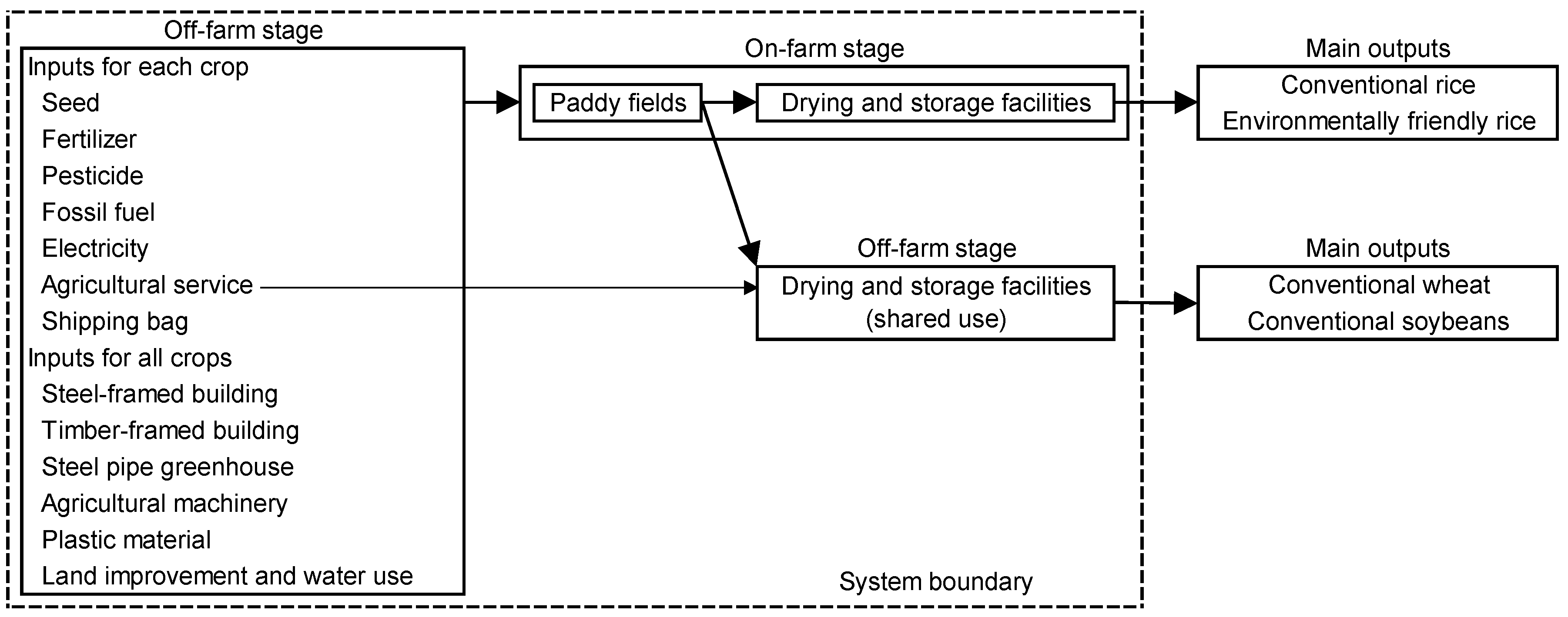
2.4. Life Cycle Assessment

Life cycle assessment (LCA) can play a useful role in environmental management in relation to products [31]. The goal of the present LCA was to calculate the total global warming potential (GWP) in the modeled farm. Because the optimized crop-planted areas were obtained by solving the optimization model, the GWP intensities for crop production were referenced to an area-based functional unit (per ha). Furthermore, the GWP intensity from the fixed and common costs was calculated. On- and off-farm emissions of three primary GHGs (CO₂, CH₄, and N₂O) were taken into account. The system boundary was the farm gate of the modeled farm (Figure 1). There was no allocation of GHG emissions between outputs and by-products because all crop residues were assumed to be contained in the farmland. A soil carbon budget in paddy fields has a positive or negative impact on GWP evaluation [32]. However, carbon sequestration or loss in the soil were excluded because of the lack of detailed data on soil conditions in the modeled farm based on farm management handbooks [21,25].

The total GWP is calculated as

$$TGWP={\displaystyle \sum _{i=1}^{11}GW{P}_i}{x^{\prime }}_i+GW{P}_{FCC}$$

(17)

where TGWP is the total GWP intensity (t CO₂ eq.); GWP_i is the ith GWP coefficient for crop production (t CO₂ eq. per ha); x’_i is the ith model-optimized planted area (ha); and GWP_FCC is the GWP intensity from the fixed and common costs (t CO₂ eq.).

Table 5. Inventory data on crop production in the modeled farm (per ha).

	CR				EFR				CW	CS
	VEV	EV	MV	LV	VEV	EV	MV	LV	MV	MV	LV
Fossil fuel (L) 1
Gasoline	126.0	131.0	136.0	141.0	121.0	126.0	131.0	136.0	25.0	15.0	15.0
Diesel oil	182.0	182.0	182.0	182.0	182.0	182.0	182.0	182.0	185.0	161.0	161.0
Premixed fuel (25:1)	15.8	15.8	15.8	15.8	14.8	14.8	14.8	14.8	7.2	6.4	6.4
Motor oil	20.0	20.0	20.0	20.0	20.0	20.0	20.0	20.0	10.0	10.0	10.0
Kerosene	180.0	150.0	90.0	90.0	180.0	150.0	90.0	90.0	0	0	0
Production cost (thousand yen) 2
Seed	16.5	18.0	16.5	16.5	16.5	18.0	16.5	16.5	30.4	31.5	32.5
Chemical fertilizer	107.5	107.5	107.5	107.5	125.9	125.9	125.9	125.9	97.2	79.4	79.4
Organic fertilizer	0	0	0	0	50.8	50.8	50.8	50.8	0	0	0
Pesticide	58.3	58.3	58.3	58.3	64.6	64.6	64.6	64.6	28.6	53.1	53.1
Fossil fuel	64.8	62.9	58.2	58.9	63.9	62.0	57.3	58.0	26.2	22.7	22.7
Electricity	0.9	0.8	0.6	0.6	0.9	0.8	0.6	0.6	0.001	0	0
Agricultural service	34.6	34.6	34.6	34.6	17.3	17.3	17.3	17.3	126.0	63.0	63.0
Shipping bag	12.7	13.5	14.3	12.7	11.5	12.3	13.0	11.5	0	5.3	5.3
Others	19.6	19.6	19.6	19.6	19.6	19.6	19.6	19.6	14.7	15.7	15.7
Nitrogen input (kg N) 3
Chemical fertilizer	80.0	80.0	80.0	80.0	40.0	40.0	40.0	40.0	148.0	20.0	20.0
Organic fertilizer	0	0	0	0	40.0	40.0	40.0	40.0	0	0	0
Nitrogen fixation by legumes	0	0	0	0	0	0	0	0	0	121.1	121.1
Crop residue	30.2	32.1	34.0	30.2	27.4	29.1	30.9	27.4	19.5	9.6	9.6
Magnesium carbonate fertilizer (t) 4	0	0	0	0	0	0	0	0	1.0	1.0	1.0

CR = conventional rice, EFR = environmentally friendly rice, CW = conventional wheat, CS = conventional soybeans, VEV = very early variety, EV = early variety, MV = medium variety, and LV = late variety; ¹ The amounts of fossil fuels were calculated based on each cultivation protocol [21,25]; ² The production costs, apart from those of fertilizer and pesticide in conventional rice production (average in 2010–2012 [29]), were calculated based on each cultivation protocol [21,25]. In environmentally friendly rice production, the cost of organic–inorganic compound fertilizer was allocated between chemical fertilizer and organic fertilizer based on their nitrogen contents. Others included the costs of nursery soil for rice production and crop insurance for each crop, but they were excluded from the present LCA because there were no environmental burden coefficients; ³ The nitrogen inputs of chemical and organic fertilizers were calculated based on each fertilizer recommendation [21,26,35]. Those of crop residues were calculated using the dry-matter contents of yields (rice 84.5%, wheat 87.5%, and soybeans 87.5% [36]), the ratios of crop residues to harvested crops on a dry-matter basis (rice 105.9%, wheat 144.9%, and soybeans 82.8% [37]), and the nitrogen contents of crop residues on a dry-matter basis (rice 0.7%, wheat 0.4%, and soybeans 0.7% [37]). The nitrogen fixation rate of soybeans was assumed to be equal to the total nitrogen contained in the yield and crop residue [7]. The nitrogen yields of soybeans were calculated using the dry-matter content (87.5%) of yield [36] and the nitrogen content (6.4%) of yield on a dry-matter basis [37]; ⁴ These values were cited from Shiga Prefecture [21].

and

Table 6. Fixed and common costs of the modeled farm (million yen per year) ¹.

Item	Cost
Steel-framed building	1.53
Timber-framed building	0.28
Steel pipe greenhouse	0.26
Agricultural machinery	10.49
Plastic material	0.28
Land improvement and water use	1.03
Others 2	2.69

¹ These costs were taken from a Shiga Prefecture handbook [21]; ² Others included the land rent, taxes and dues, and other costs, but they were excluded from the present LCA because there were no environmental burden coefficients. Land rent and taxes and dues, which did not contribute to off-farm GHG emissions, accounted for 93% of the cost in Others.

show the data collected for the present LCA. On-farm GHGs were emitted from fossil fuel combustion, nitrogen input, agricultural lime application, and rice paddy fields. The GHG emissions from fossil fuel combustion were calculated using the CO₂, CH₄, and N₂O emission factors [7]. For nitrogen input, the N₂O emission factors were 0.31% N₂O-N in fertilization for rice production, 0.62% N₂O-N in fertilization for wheat and soybean production and nitrogen fixation by soybean cultivars, and 1.25% N₂O-N in crop residue incorporation [7]. The CO₂ emission factor of magnesium carbonate fertilizers was 13% CO₂-C [7]. The CH₄ emission rate from rice paddy fields with conventional midseason drainage was 181.2 kg per ha per year, weighted by the ratios of soil types in the Shiga region [7,33], while that with prolonged midseason drainage was assumed to be reduced to 69.5% [10]. Variation in the N₂O emissions resulting from prolonged midseason drainage was not taken into account because N₂O emissions from rice paddy fields, in terms of GWP-based CO₂ equivalent, were much smaller than CH₄ emissions [10]. Off-farm emissions of CO₂, CH₄, and N₂O were calculated using the cost data and the embodied global environmental burden coefficients based on the purchaser price of household consumption expenditure or producer price in 2005 [34].

The CO₂ equivalence factors for GWP were CO₂ 1, CH₄ 21, and N₂O 310 on a 100-year time horizon [38], which were equal to those used in studies by Nansai et al. [34] and the Greenhouse Gas Inventory Office of Japan [7].

2.5. Eco-Efficiency

Eco-efficiency is a key concept that involves achieving more value from fewer inputs of materials and energy and with reduced emissions, and is a means of making and measuring progress toward economic and environmental sustainability [39]. Eco-efficient farming is concerned with the efficient and sustainable use of resources in agricultural production and land management [3]. The eco-efficiency indicators that were used to bring together net farm income and GWP were calculated as

$$EE=\frac{NF{I}_{\mathit{max}}}{TGWP}$$

(18)

where EE is the eco-efficiency (million yen per t CO₂ eq.) and NFI_max is the maximized net farm income (million yen).

3. Results

3.1. Global Warming Impact in the Modeled Farm

Table 7. LCA results of the modeled farm (kg CO₂ eq. per ha for each crop; kg CO₂ eq. for fixed and common costs).

	CR				EFR				CW	CS		FCC
	VEV	EV	MV	LV	VEV	EV	MV	LV	MV	MV	LV
Seed	53	58	53	53	53	58	53	53	98	101	104
Fertilizer	1205	1205	1205	1205	1560	1560	1560	1560	1904	1338	1338
Pesticide	278	278	278	278	308	308	308	308	137	253	253
Fossil fuel	1718	1643	1476	1492	1698	1623	1456	1472	751	641	641
Electricity	26	23	18	18	27	24	18	18	0.04	0	0
Agricultural service	121	121	121	121	61	61	61	61	441	220	220
Shipping bag	45	48	51	45	41	44	46	41	0	19	19
CH4 from rice paddy fields	3804	3804	3804	3804	2644	2644	2644	2644	0	0	0
Nitrogen fixation by legumes	0	0	0	0	0	0	0	0	0	366	366
Crop residue	184	196	207	184	167	177	188	167	119	58	58
Steel-framed building												6439
Timber-framed building												879
Steel pipe greenhouse												4584
Agricultural machinery												44,817
Plastic material												975
Land improvement and water use												3587
Total	7435	7376	7213	7200	6560	6499	6335	6325	3449	2997	3000	61,282

CR = conventional rice, EFR = environmentally friendly rice, CW = conventional wheat, CS = conventional soybeans, VEV = very early variety, EV = early variety, MV = medium variety, LV = late variety, and FCC = fixed and common costs.

shows the GWP intensities of each crop and for fixed and common costs in the modeled farm. A contribution analysis was performed to identify environmental hot spots. Because the LCA components such as system definition, GHG emission coefficients, and CO₂ equivalence factors differ, it is difficult to compare these results with the GWP intensities in previous LCA studies.

GHG emissions from environmentally friendly rice production were smaller than those from conventional rice production. As noted in previous studies [40,41,42,43,44], the major contribution (40%–53%) to GHG emissions from rice production came from CH₄ emitted from rice paddy fields. Thus, prolonged midseason drainage that can substantially reduce CH₄ emissions from rice paddy fields [10] is especially important for ensuring the environmental advantage for environmentally friendly rice production.

Use of fertilizers was the primary contributor to the GWP intensities in both wheat (55%) and soybeans (45%) produced conventionally. Because a large quantity of fertilizers is required for high-yield wheat production with an increased grain protein content [45], chemical fertilizer production and field emissions from fertilizer application are the environmental hot spots for conventional wheat production [46,47,48,49]. Although some studies have indicated that diesel combustion is the major source of global warming impacts on soybean production [50,51], the results of the present LCA confirmed the impacts reported by Pelletier et al. [48]. The GWP intensity of agricultural machinery production, which is the primary contributor to GHG emissions in farm capital [52], accounted for 73% of the total GWP in fixed and common costs.

3.2. Model-Optimized Results

The model-optimized results of land use and temporary workers were very similar between the CR and EFR farms (

Table 8. Model-optimized results.

	CR Farm	EFR Farm
Land use (ha)
CR (VEV)	0
CR (EV)	5.0
CR (MV)	8.5
CR (LV)	0
EFR (VEV)		0
EFR (EV)		5.0
EFR (MV)		8.5
EFR (LV)		0
CW (MV)	13.5	13.5
CS (MV)	8.6	8.6
CS (LV)	4.9	4.9
Temporary workers (hours)
Early June	43.5	43.5
Early July	0	0
Late July	35.5	35.5
Mid-August	0	0
Late September	0	0
Economic, environmental, and integrated indicators
Net farm income (million yen)	7.76	7.08
GWP (t CO2 eq.)	246.5	234.6
Eco-efficiency (million yen per t CO2 eq.)	0.031	0.030

CR farm = modeled farm with conventional rice production, EFR farm = modeled farm with environmentally friendly rice production, CR = conventional rice, EFR = environmentally friendly rice, CW = conventional wheat, CS = conventional soybeans, VEV = very early variety, EV = early variety, MV = medium variety, and LV = late variety.

). Under net farm income maximization, both farms selected early- and medium-maturing rice varieties that generated larger crop incomes compared with very early- and late-maturing rice varieties, and reduced rice cultivation to 50% of the total farmland because the total crop income from a wheat–soybean rotation, which depended on a large subsidy, was greater than that from a rice cultivation (Table 3) [53]. In both farms, family labor resources were exhausted in early June, early July, and late July, and additional labor inputs from temporary workers were required to avoid labor shortages in early June and late July.

4. Discussion

4.1. Comparison between Two Modeled Farms

To address the first research question (whether Japanese rice farms have some advantages in producing environmentally friendly rice under the current conditions), comparisons of net farm income, GWP, and eco-efficiency between the CR and EFR farms were made based on the model-optimized results under the current conditions (Table 8). The differences in the three indicators between the CR and EFR farms were affected by different rice cultivation methods because the wheat and soybean areas cultivated and the number of temporary workers hired in both farms were the same. Compared with the CR farm, the EFR farm generated smaller net farm income, while it contributed to mitigating global warming. From an eco-efficiency perspective, there was no advantage for the EFR farm.

The second research question examined whether net farm income, GWP, and eco-efficiency for the EFR farm were improved by an increase in the direct payments for environmentally friendly rice production (Figure 2). Even though the optimization problems were iteratively solved when the direct payments increased from 40,000 (base) to 100,000 yen per ha, there were no changes in the model-optimized results of land use and temporary workers, as shown in Table 8. The net farm income and eco-efficiency of the EFR farm were greater than those of the CR farm when the direct payments were 91,000 and 64,000 yen per ha, respectively. However, the GWP intensities from the EFR farm were the same under any level of direct payment because there were no changes in its land use pattern.

These findings suggest that under the current level of direct payment, the practice of prolonged midseason drainage in environmentally friendly rice production causes larger economic disadvantages in exchange for smaller environmental advantages. If farmers pursue maximum agricultural profit as assumed in the optimization model, conventional rice farmers should not switch to environmentally friendly rice production with prolonged midseason drainage. Environmentally friendly rice farmers will also find it difficult to adopt a prolonged midseason drainage technique because rice yield reductions caused by prolonging midseason drainage are not compensated sufficiently by the current direct payment.

There are several reasons why a prolonged midseason drainage technique in producing environmentally friendly rice is practiced in most of the areas supported by the direct payment program for environmentally friendly agriculture in the Shiga region. First, regarding the technical aspects, farmers who have produced environmentally friendly rice can easily adopt the local special practices including integrated pest management, mechanical weeding at paddy field dikes, and prolonged midseason drainage involving the cutting of furrows. This is because every technique except for prolonged midseason drainage has already been introduced in the cultivation protocols of environmentally friendly rice [21] and the operations of prolonged midseason drainage are much the same as those of conventional midseason drainage [22,26]. Second, when farmers in the Shiga region adopt environmentally friendly farming techniques, most of them primarily aim to supply safe and secure agricultural produce and conserve the environment, including Lake Biwa [28,54]. Such farmers appear to accept the risk of yield variations for environmentally friendly rice with prolonged midseason drainage. Unlike the optimization model, the problem that they face may be expressed as a multi-objective function [11,20], in which the weights of environmental factors are larger than those of economic factors. However, when they are no longer able to endure such risk, they stop practicing prolonged midseason drainage.

The Ministry of Agriculture, Forestry and Fisheries of Japan does not elaborate on how to determine the current direct payment rates for environmentally friendly agriculture [5]. Given that the government gives farmers subsidy payments for agricultural environmental services to provide economic incentives for the adoption of eco-efficient systems [3], the direct payment rates for environmentally friendly agriculture should be determined based on the condition that environmentally friendly agricultural practices improve eco-efficiency compared with conventional agriculture. Thus, based on eco-efficiency indicators, an increase in the direct payment rate for environmentally friendly rice production with prolonged midseason drainage is required to reduce the risk of yield variations, and to provide the environmental benefit of reducing CH₄ emissions from rice paddy fields sustainably.

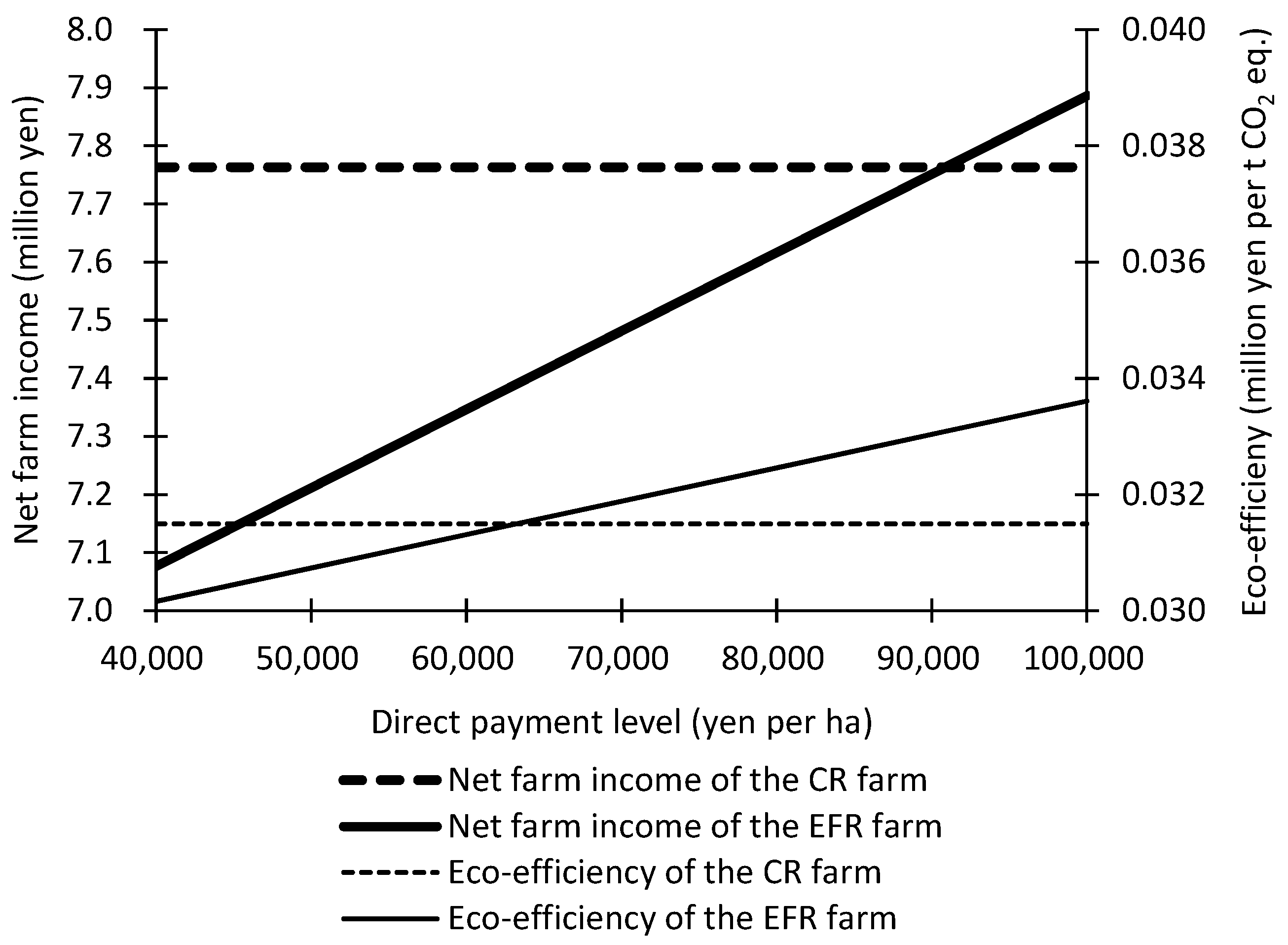
4.2. Sensitivity Analysis on the CO₂ Equivalence Factors

Because the indirect GHG emission coefficients from Nansai et al. [34] were converted in terms of CO₂ equivalence using the characterization factors in the Greenhouse Gas Inventory Office of Japan [7,55], 1 of CO₂, 21 of CH₄, and 310 of N₂O on a 100-year time horizon were selected for GWP assessment in this paper. In the sensitivity analysis, the GWP results that were recalculated using the new CO₂ equivalence factors, CO₂ 1, CH₄ 28, and N₂O 265 on a 100-year time horizon [6], were compared with those shown in Table 7.

When the new CO₂ equivalence factors were used, the GWP results of conventional rice, environmentally friendly rice, conventional wheat, and conventional soybeans were 8449–8684, 7195–7430, 3388, and 2944–2948 kg CO₂ eq. per ha, respectively, and that of fixed and common costs was 61,626 kg CO₂ eq. The recalculated GWP intensities for rice production were greater than the GWP results shown in Table 7 because a larger CO₂ equivalence factor for CH₄ contributed to an increase in the GWP intensities for rice production with CH₄ from rice paddy fields as the major emission source. However, not much difference was found between the recalculated results and the present results (Table 7) in other categories. Given the model-optimized results of land use (Table 8), the GWP intensities of the CR and EFR farms under the new CO₂ equivalence factors were 262.1 and 245.2 t CO₂ eq., respectively.

As with the results of eco-efficiency shown in Table 8, the eco-efficiency value (0.030 million yen per t CO₂ eq.) of the CR farm in the recalculation was greater than that (0.029 million yen per t CO₂ eq.) of the EFR farm. Thus, even with the use of the new CO₂ equivalence factors, the fact remains that an increase in the direct payment rate is important for improving eco-efficiency in the EFR farm.

4.3. Eco-Efficiency Measurement Methodologies

In this paper, the eco-efficiency of the modeled farm was calculated by a combination of the results of linear programming and LCA. This method enables us to measure an eco-efficiency score with respect to each environmental impact category such as GWP. In contrast, to create a comprehensive eco-efficiency indicator, other papers have proposed data envelopment analysis (DEA)-based eco-efficiency using multiple environmental impacts or life cycle inventory data [56,57,58,59]. A number of studies have confirmed the effectiveness of a combined application of LCA and DEA in aggregate eco-efficiency assessment of agricultural production (e.g., [57,60,61,62]). Although DEA-based eco-efficiency measurement is useful for comprehensive eco-efficiency assessment, it requires a large sample size for the DEA calculation. Compared with DEA-based eco-efficiency measurement, eco-efficiency measurement from farm modeling based on farm management handbooks in this paper has the advantage of lower data requirements.

5. Conclusions

The economic and environmental effects of agri-environmental direct payments when Japanese rice farmers adopted a prolonged midseason drainage technique to mitigate global warming were examined using a combined application of an optimization model and LCA at a farm scale. A modeled farm that produced environmentally friendly rice with prolonged midseason drainage was compared with a modeled farm that produced conventional rice with normal midseason drainage. Eco-efficiency was used as an integrated indicator for assessing the economic and environmental feasibilities.

The results showed that under the current direct payment level, a prolonged midseason drainage technique has no benefit in improving the eco-efficiency of Japanese rice farms because the practice of this technique in environmentally friendly rice production causes larger economic disadvantages in exchange for smaller environmental advantages. In the adoption of this technique, an increase in the direct payment rate is required to reduce the risk of rice yield variations, and to enhance eco-efficiency. Because improvement of eco-efficiency in adopting agri-environmental measures is the most important goal for agri-environmental payments, given budget constraints, the direct payment rates for agri-environmental measures should be determined based on eco-efficiency improvement compared with conventional agriculture.

References

1. Latacz-Lohmann, U.; Hodge, I. European agri-environmental policy for the 21st century. Aust. J. Agric. Resour. Econ. 2003, 47, 123–139. [Google Scholar] [CrossRef]
2. Organisation for Economic Co-Operation and Development. Evaluation of Agricultural Policy Reforms in the European Union; OECD Publishing: Paris, France, 2011. [Google Scholar]
3. Wilkins, R.J. Eco-efficient approaches to land management: A case for increased integration of crop and animal production systems. Philos. Trans. R. Soc. B 2008, 363, 517–525. [Google Scholar] [CrossRef] [PubMed]
4. Ministry of Agriculture, Forestry and Fisheries of Japan. The Direct Payment Program for Environmentally Friendly Agriculture. Available online: http://www.maff.go.jp/j/seisan/kankyo/kakyou_chokubarai/mainp.html (accessed on 11 August 2014). (In Japanese)
5. Nishizawa, E. Agri-environmental policies in Japan and environmentally friendly agriculture in the Shiga region. In Economic Analysis of Agri-Environmental Policies; Nishizawa, E., Ed.; Nippon Hyoron Sha: Tokyo, Japan, 2014; pp. 99–120. (In Japanese) [Google Scholar]
6. Stocker, T.F.; Qin, D.; Plattner, G.-K.; Tignor, M.M.B.; Allen, S.K.; Boschung, J.; Nauels, A.; Xia, Y.; Bex, V.; Midgley, P.M. (Eds.) Climate Change 2013: The Physical Science Basis; Cambridge University Press: Cambridge, UK, 2013.
7. Greenhouse Gas Inventory Office of Japan. National Greenhouse Gas Inventory Report of Japan; National Institute for Environmental Studies: Tsukuba, Japan, 2014. [Google Scholar]
8. Food and Agriculture Organization of the United Nations. FAOSTAT: Emissions-Agriculture. Available online: http://faostat3.fao.org/download/G1/*/E (accessed on 22 January 2015).
9. Yagi, K.; Tsuruta, H.; Minami, K. Possible options for mitigating methane emission from rice cultivation. Nutr. Cycl. Agroecosyst. 1997, 49, 213–220. [Google Scholar] [CrossRef]
10. Itoh, M.; Sudo, S.; Mori, S.; Saito, H.; Yoshida, T.; Shiratori, Y.; Suga, S.; Yoshikawa, N.; Suzue, Y.; Mizukami, H.; et al. Mitigation of methane emissions from paddy fields by prolonging midseason drainage. Agric. Ecosyst. Environ. 2011, 141, 359–372. [Google Scholar] [CrossRef]
11. Chono, S.; Maeda, S.; Kawachi, T.; Imagawa, C.; Buma, N.; Takeuchi, J. Optimization model for cropping-plan placement in paddy fields considering agricultural profit and nitrogen load management in Japan. Paddy Water Environ. 2012, 10, 113–120. [Google Scholar] [CrossRef] [Green Version]
12. Senthilkumar, K.; Lubbers, M.T.M.H.; de Ridder, N.; Bindraban, P.S.; Thiyagarajan, T.M.; Giller, K.E. Policies to support economic and environmental goals at farm and regional scales: Outcomes for rice farmers in Southern India depend on their resource endowment. Agric. Syst. 2011, 104, 82–93. [Google Scholar] [CrossRef]
13. Glithero, N.J.; Ramsden, S.J.; Wilson, P. Farm systems assessment of bioenergy feedstock production: Integrating bio-economic models and life cycle analysis approaches. Agric. Syst. 2012, 109, 53–64. [Google Scholar] [CrossRef] [PubMed]
14. Nakashima, T. Life cycle assessment integrated into positive mathematical programming: A conceptual model for analyzing area-based farming policy. Jpn. Agric. Res. Q. 2010, 44, 301–310. [Google Scholar] [CrossRef]
15. Louhichi, K.; Kanellopoulos, A.; Janssen, S.; Flichman, G.; Blanco, M.; Hengsdijk, H.; Heckelei, T.; Berentsen, P.; Lansink, A.O.; van Ittersum, M. FSSIM, a bio-economic farm model for simulating the response of EU farming systems to agricultural and environmental policies. Agric. Syst. 2010, 103, 585–597. [Google Scholar] [CrossRef] [Green Version]
16. Schader, C.; Lampkin, N.; Christie, M.; Nemecek, T.; Gaillard, G.; Stolze, M. Evaluation of cost-effectiveness of organic farming support as an agri-environmental measure at Swiss agricultural sector level. Land Use Policy 2013, 31, 196–208. [Google Scholar] [CrossRef]
17. Berentsen, P.B.M.; Giesen, G.W.J. An environmental–economic model at farm level to analyse institutional and technical change in dairy farming. Agric. Syst. 1995, 49, 153–175. [Google Scholar] [CrossRef]
18. Berentsen, P.B.M.; Tiessink, M. Potential effects of accumulating environmental policies on Dutch dairy farms. J. Dairy Sci. 2003, 86, 1019–1028. [Google Scholar] [CrossRef]
19. Van Calker, K.J.; Berentsen, P.B.M.; de Boer, I.M.J.; Giesen, G.W.J.; Huirne, R.B.M. An LP-model to analyse economic and ecological sustainability on Dutch dairy farms: Model presentation and application for experimental farm “de Marke”. Agric. Syst. 2004, 82, 139–160. [Google Scholar] [CrossRef]
20. Zimmermann, A. Optimization of sustainable dairy-cow feeding systems with an economic-ecological LP farm model using various optimization processes. J. Sustain. Agric. 2008, 32, 77–94. [Google Scholar] [CrossRef]
21. Shiga Prefecture. Handbook on Agricultural Management, 2012 ed.; Shiga Prefecture: Otsu, Japan, 2012. (In Japanese) [Google Scholar]
22. Shiga Prefecture. Direct Payments for Environmentally Friendly Agriculture. Available online: http://www.pref.shiga.lg.jp/g/kodawari/kodawarishien.html (accessed on 26 August 2014). (In Japanese)
23. Ministry of Agriculture, Forestry and Fisheries of Japan. The Implementation Status of the Direct Payment Program for Environmentally Friendly Agriculture in 2013. Available online: http://www.maff.go.jp/j/seisan/kankyo/kakyou_chokubarai/pdf/25_jisseki2.pdf (accessed on 23 February 2016). (In Japanese)
24. Shiga Prefecture; Shiga Prefecture. personal communication, 2013–2014.
25. Shiga Prefecture. Handbook on Agricultural Management, 2002 ed.; Shiga Prefecture: Otsu, Japan, 2002. (In Japanese) [Google Scholar]
26. Shiga Prefecture. Technical Guide on Rice Production; Shiga Prefecture: Otsu, Japan, 2010. (In Japanese) [Google Scholar]
27. Ministry of Agriculture, Forestry and Fisheries of Japan. Summary of the Income Stabilization Program for Farmers in 2014. Available online: http://www.maff.go.jp/j/kobetu_ninaite/keiei/pdf/26pamph_all.pdf (accessed on 11 August 2014). (In Japanese)
28. Kurosawa, M.; Tezuka, T. Awareness of farmers approaching the sustainable agriculture to improve regional environment: Case study of environmentally conscious agriculture in Shiga Prefecture. J. Rural Plan. Assoc. 2005, 24, 61–66, (In Japanese with English Abstract). [Google Scholar] [CrossRef]
29. Ministry of Agriculture, Forestry and Fisheries of Japan. Statistics of Production Costs of Crops. Available online: http://www.maff.go.jp/j/tokei/kouhyou/noukei/seisanhi_nousan/ (accessed on 29 August 2014). (In Japanese)
30. Oishi, W. Linear programming program “XLP” for farming planning. Agric. Inf. Res. 2006, 15, 319–330, (In Japanese with English Abstract). [Google Scholar] [CrossRef]
31. Guinée, J.B. (Ed.) Handbook on Life Cycle Assessment: Operational Guide to the ISO Standards; Kluwer Academic Publishers: Dordrecht, The Netherlands, 2002.
32. Nishimura, S.; Yonemura, S.; Sawamoto, T.; Shirato, Y.; Akiyama, H.; Sudo, S.; Yagi, K. Effect of land use change from paddy rice cultivation to upland crop cultivation on soil carbon budget of a cropland in Japan. Agric. Ecosyst. Environ. 2008, 125, 9–20. [Google Scholar] [CrossRef]
33. Shiga Prefecture. Technical Guide on Soil Preparation; Shiga Prefecture: Otsu, Japan, 2001. (In Japanese) [Google Scholar]
34. Nansai, K.; Kondo, Y.; Kagawa, S.; Suh, S.; Nakajima, K.; Inaba, R.; Tohno, S. Estimates of embodied global energy and air-emission intensities of Japanese products for building a Japanese input-output life cycle assessment database with a global system boundary. Environ. Sci. Technol. 2012, 46, 9146–9154. [Google Scholar] [CrossRef] [PubMed]
35. Shiga Prefecture. Technical Guide on Environmentally Friendly Agriculture; Shiga Prefecture: Otsu, Japan, 2010. (In Japanese) [Google Scholar]
36. Ministry of Education, Culture, Sports, Science and Technology of Japan. Food Composition Database. Available online: http://fooddb.mext.go.jp/index.pl (accessed on 29 August 2014). (In Japanese)
37. Owa, N. Nutrient balances of crops in Japan. Kanhonokenren News 1996, 33, 428–445. (In Japanese) [Google Scholar]
38. Houghton, J.T.; Meira Filho, L.G.; Callander, B.A.; Harris, N.; Kattenberg, A.; Maskell, K. (Eds.) Climate Change 1995: The Science of Climate Change; Cambridge University Press: Cambridge, UK, 1996.
39. Verfaillie, H.A.; Bidwell, R. Measuring Eco-Efficiency: A Guide to Reporting Company Performance; World Business Council for Sustainable Development: Geneva, Switzerland, 2000. [Google Scholar]
40. Breiling, M.; Hashimoto, S.; Sato, Y.; Ahamer, G. Rice-related greenhouse gases in Japan, variations in scale and time and significance for the Kyoto Protocol. Paddy Water Environ. 2005, 3, 39–46. [Google Scholar] [CrossRef]
41. Harada, H.; Kobayashi, H.; Shindo, H. Reduction in greenhouse gas emissions by no-tilling rice cultivation in Hachirogata polder, northern Japan: Life-cycle inventory analysis. Soil Sci. Plant Nutr. 2007, 53, 668–677. [Google Scholar] [CrossRef]
42. Hokazono, S.; Hayashi, K. Variability in environmental impacts during conversion from conventional to organic farming: A comparison among three rice production systems in Japan. J. Clean. Prod. 2012, 28, 101–112. [Google Scholar] [CrossRef]
43. Koga, N.; Tajima, R. Assessing energy efficiencies and greenhouse gas emissions under bioethanol-oriented paddy rice production in northern Japan. J. Environ. Manag. 2011, 92, 967–973. [Google Scholar] [CrossRef] [PubMed]
44. Wang, M.; Xia, X.; Zhang, Q.; Liu, J. Life cycle assessment of a rice production system in Taihu region, China. Int. J. Sustain. Dev. World Ecol. 2010, 17, 157–161. [Google Scholar] [CrossRef]
45. Shiga Prefecture. Guide for Producing Salable Wheat and Soybeans; Shiga Prefecture: Otsu, Japan, 2012. (In Japanese) [Google Scholar]
46. Biswas, W.K.; Barton, L.; Carter, D. Global warming potential of wheat production in Western Australia: A life cycle assessment. Water Environ. J. 2008, 22, 206–216. [Google Scholar] [CrossRef]
47. Charles, R.; Jolliet, O.; Gaillard, G.; Pellet, D. Environmental analysis of intensity level in wheat crop production using life cycle assessment. Agric. Ecosyst. Environ. 2006, 113, 216–225. [Google Scholar] [CrossRef]
48. Pelletier, N.; Arsenault, N.; Tyedmers, P. Scenario modeling potential eco-efficiency gains from a transition to organic agriculture: Life cycle perspectives on Canadian canola, corn, soy, and wheat production. Environ. Manag. 2008, 42, 989–1001. [Google Scholar] [CrossRef] [PubMed]
49. Tuomisto, H.L.; Hodge, I.D.; Riordan, P.; Macdonald, D.W. Comparing global warming potential, energy use and land use of organic, conventional and integrated winter wheat production. Ann. Appl. Biol. 2012, 161, 116–126. [Google Scholar] [CrossRef]
50. Castanheira, É.G.; Freire, F. Greenhouse gas assessment of soybean production: Implications of land use change and different cultivation systems. J. Clean. Prod. 2013, 54, 49–60. [Google Scholar] [CrossRef]
51. Kim, S.; Dale, B.E. Cumulative energy and global warming impact from the production of biomass for biobased products. J. Ind. Ecol. 2003, 7, 147–162. [Google Scholar] [CrossRef]
52. Korsaeth, A.; Jacobsen, A.Z.; Roer, A.-G.; Henriksen, T.M.; Sonesson, U.; Bonesmo, H.; Skjelvåg, A.O.; Strømman, A.H. Environmental life cycle assessment of cereal and bread production in Norway. Acta Agric. Scand. A 2012, 62, 242–253. [Google Scholar] [CrossRef]
53. Hokazono, S.; Hayashi, K. Life cycle assessment of organic paddy rotation systems using land- and product-based indicators: A case study in Japan. Int. J. Life Cycle Assess. 2015, 20, 1061–1075. [Google Scholar] [CrossRef]
54. Fujie, T. Factors influencing the adoption of environmentally friendly agriculture in the Shiga region. In Economic Analysis of Agri-Environmental Policies; Nishizawa, E., Ed.; Nippon Hyoron Sha: Tokyo, Japan, 2014; pp. 123–152. (In Japanese) [Google Scholar]
55. Nansai, K. Estimation Methods of Sectoral Energy Consumption and Greenhouse Gas Emissions Based on 2005 Input-Output Tables, Revised Edition (August 2013). Available online: http://www.cger.nies.go.jp/publications/report/d031/jpn/pdf/6/3EID2005_Method_jp.pdf (accessed on 2 June 2016). (In Japanese)
56. Kuosmanen, T.; Kortelainen, M. Measuring eco-efficiency of production with data envelopment analysis. J. Ind. Ecol. 2005, 9, 59–72. [Google Scholar] [CrossRef]
57. Iribarren, D.; Vázquez-Rowe, I.; Moreira, M.T.; Feijoo, G. Further potentials in the joint implementation of life cycle assessment and data envelopment analysis. Sci. Total Environ. 2010, 408, 5265–5272. [Google Scholar] [CrossRef] [PubMed]
58. Vázquez-Rowe, I.; Iribarren, D.; Moreira, M.T.; Feijoo, G. Combined application of life cycle assessment and data envelopment analysis as a methodological approach for the assessment of fisheries. Int. J. Life Cycle Assess. 2010, 15, 272–283. [Google Scholar] [CrossRef]
59. Tatari, O.; Kucukvar, M. Eco-efficiency of construction materials: Data envelopment analysis. J. Constr. Eng. Manag. 2012, 138, 733–741. [Google Scholar] [CrossRef]
60. Jan, P.; Dux, D.; Lips, M.; Alig, M.; Dumondel, M. On the link between economic and environmental performance of Swiss dairy farms of the alpine area. Int. J. Life Cycle Assess. 2012, 17, 706–719. [Google Scholar] [CrossRef]
61. Mohammadi, A.; Rafiee, S.; Jafari, A.; Keyhani, A.; Dalgaard, T.; Knudsen, M.T.; Nguyen, T.L.T.; Borek, R.; Hermansen, J.E. Joint life cycle assessment and data envelopment analysis for the benchmarking of environmental impacts in rice paddy production. J. Clean. Prod. 2015, 106, 521–532. [Google Scholar] [CrossRef]
62. Masuda, K. Measuring eco-efficiency of wheat production in Japan: A combined application of life cycle assessment and data envelopment analysis. J. Clean. Prod. 2016, 126, 373–381. [Google Scholar] [CrossRef]
Figure 1. A simplified flowchart of crop production in the modeled farm.
Sustainability 08 00593 g001
Figure 2. Effects of gradually increasing direct payment levels on net farm income and eco-efficiency. CR farm = modeled farm with conventional rice production; EFR farm = modeled farm with environmentally friendly rice production.
Sustainability 08 00593 g002