Issues of Application of Machine Learning Models for Virtual and Real-Life Buildings

Abstract

The current Building Energy Performance Simulation (BEPS) tools are based on first principles. For the correct use of BEPS tools, simulationists should have an in-depth understanding of building physics, numerical methods, control logics of building systems, etc. However, it takes significant time and effort to develop a first principles-based simulation model for existing buildings—mainly due to the laborious process of data gathering, uncertain inputs, model calibration, etc. Rather than resorting to an expert’s effort, a data-driven approach (so-called “inverse” approach) has received growing attention for the simulation of existing buildings. This paper reports a cross-comparison of three popular machine learning models (Artificial Neural Network (ANN), Support Vector Machine (SVM), and Gaussian Process (GP)) for predicting a chiller’s energy consumption in a virtual and a real-life building. The predictions based on the three models are sufficiently accurate compared to the virtual and real measurements. This paper addresses the following issues for the successful development of machine learning models: reproducibility, selection of inputs, training period, outlying data obtained from the building energy management system (BEMS), and validation of the models. From the result of this comparative study, it was found that SVM has a disadvantage in computation time compared to ANN and GP. GP is the most sensitive to a training period among the three models.

1. Introduction

Classical forward models—known as dynamic building simulation models—have been used over the last several decades. However, several unsolved issues remain: uncertainty in prediction, time consuming and demanding effort to develop an accurate (calibrated) model, handling of unknown inputs (e.g., missing information), and transparency of the model [1].

An inverse (data-driven) model has been regarded as an alternative to the forward approach, especially for the modeling of existing buildings. Compared to the forward model, the inverse model can be developed with significantly fewer inputs and less time and effort. For the inverse approach, machine-learning techniques such as Artificial Neural Network (ANN) [2], Support Vector Machine (SVM) [3,4], and Gaussian Process (GP) [5] can be used. Especially, the Gaussian Process (GP) has received growing attention because of its stochastic prediction capability (e.g., confidence internal) [5,6].

A comparison between the forward models and the inverse models was conducted [7,8]. Neto et al. [7] developed a detailed EnergyPlus simulation model and an ANN model to predict the entire building energy consumption for an office building. They used weather data as inputs and the results showed that both models had good agreement with real measurements. Cam et al. [3] cross-compared four inverse models (kernel regression, dynamic ANN, Support Vector Regression (SVR), and multi polynomial regression) to forecast the electric demand of chillers in a large institutional building. The authors identified that the models showed a coefficient of variation of less than 7% for forecasting hourly electric demand, while the SVR model performed best in the test period. Several studies compared static inverse models with dynamic inverse models [2,9,10]. Yang et al. [2] reported that an adaptive ANN model showed better performance than a static ANN model because it has a sliding window approach, being updated with real-time measured data.

In contrast to the aforementioned work [2,3,4,5,6,7,8,9,10] that mainly focused on the development processes of machine learning models, the aim of this paper is to address the lessons, insights, and issues for application of such models for virtual and existing buildings. For this purpose, three popular machine learning algorithms (ANN, SVM, and GP) were selected, applied, and compared to a virtual and a real-life building. The issues to be elaborated in the paper are as follows: reproducibility, training period, selection of inputs, missing or outlying data obtained from BEMS, and validation of the models.

2. Three Machine Learning Algorithms

2.1. Artificial Neural Network

ANN, based on a multi-layer perceptron, has been widely used to resolve engineering problems. The ANN is a computational learning model inspired by biological neurons. It consists of input, hidden, and output layers. ANN modifies the weights between each layer, then minimizes the error function defined by the difference between predictions N(w, x₁),…, N(w, x_n) and real measurements y₁,…, y_n, using a back propagation algorithm. The objective function is defined as follows:

$$\underset{w}{argmin}E\left(w\right)=1/2{\displaystyle \sum }_{i=1}^m{\left(N\left(w,x_i\right)-y_i\right)}^2$$

(1)

where w is the weight between nodes, x is an input vector, and y is a target vector. To conduct the back propagation algorithm that seeks optimal weights, the gradient descent method, the Gauss–Newton method, and the Levenberg–Marquardt method are used. In this research, the Levenberg–Marquardt method was selected due to its short computation time and stable convergence [11]. In ANN, the number of hidden layers and nodes affects the model’s performance. However, there are no explicit rules about how they should be determined [12]. In this study, the number of layers and nodes was determined based on heuristics (trial and error). The number of hidden layers was set as three, and fifteen nodes were allocated to each hidden layer.

2.2. Support Vector Machine

SVM has been used for nonlinear function estimation. SVM transforms a given data D = {(x₁, y₁),…, (x_n, y_n)} to a feature vector in a multi-dimensional space $\left\{x_1,\cdots ,x_n\right\}\to \left\{\varnothing \left(x_1\right),\cdots \varnothing \left(x_n\right)\right\}$ and then constructs a hyper-plane f(x) that maximizes the margin $2/\Vert w\Vert$ (Equations (2) and (3)). For a regression problem, SVM determines weights to create the optimal hyper-plane, which has a maximum margin that explains the prediction performance of SVM. In other words, it minimizes the error between prediction and measurement. Slack variables ${\mathsf{\xi }}^{+}\text{\hspace{0.17em}and\hspace{0.17em}}{\mathsf{\xi }}^{-}$ are established to define the error in the objective function [13]:

$$f\left(x\right)=w^T\varnothing \left(x\right)+b$$

(2)

$$\begin{array}{c}\underset{w}{argmin}1/2{\Vert w\Vert }^2+C{\sum }_{i=1}^n\left({\xi }_i{}^{+}-{\xi }_i^{-}\right)\\ subjectto\{\begin{array}{c}{y}_i-f\left(x_i\right)\le ϵ+{\xi }_i{}^{+}\\ y_i-f\left(x_i\right)\le -ϵ-{\xi }_i^{-}\\ {\xi }^{+},{\xi }^{-}\ge 0\end{array}\end{array}$$

(3)

where C is a trade-off coefficient that adjusts the hyper-plane between the margin and the error, f is a prediction output, y is a real measurement, and $ϵ$ is a free parameter that serves as a threshold.

Although the SVM is widely applied to solve regression problems due to its stability, a weakness of SVM is its computational demand to minimize the objective function with inequality constraints. In this paper, a modified model, Least Square SVM (LSSVM) was applied to overcome this drawback. LSSVM reduces inequality constraints by converting slack variables into squared error functions, e₁,…, e_i. In addition, the kernel function K substitutes the inner products of pairs of the feature vector under Mercer’s theorem. As a result, the hyper-plane and objective function of SVM (Equations (2) and (3)) are transformed as follows [14]:

$$f\left(x\right)={\displaystyle \sum }_{i=1}^n{\alpha }_{i}K\left(x,x_i\right)+b$$

(4)

$$\begin{array}{c}\underset{w}{argmin}1/2{\Vert w\Vert }^2+1/2{\gamma }^2{\displaystyle \sum }_{i=1}^n{e}_i^2\\ subjectto{y}_i=w^T\varnothing \left(x_i\right)+b+e_i\end{array}$$

(5)

While many types of kernel functions can be used, in this study, the Gaussian type of Radial Basis Function (RBF) kernel was used since it can effectively handle nonlinear problems [15].

2.3. Gaussian Process

GP is a joint distribution of random variables {f₁, f₂, …, f_n} assigned on given data {x₁, x₂,…, x_n}. When a training data set D = {(x₁, y₁), (x₂, y₂), …, (x_i, y_i)} is given, the posterior distribution of the random variables (Equation (6)) can be obtained. GP is expressed with the mean (Equation (7)) and covariance functions (Equation (8)) of random variables as follows:

$$f\left(x\right)~GP\left(m\left(x\right),k\left(x,x^{\prime }\right)\right)$$

(6)

$$m\left(x\right)=E\left[f\left(x\right)\right]$$

(7)

$$k\left(x,x^{\prime }\right)=E\left[\left(f\left(x\right)-m\left(x\right)\right)\left(f\left(x^{\prime }\right)-m\left(x^{\prime }\right)\right)\right]$$

(8)

The covariance function explains the correlation between random variables. It can be substituted with Squared Exponential (SE), Rational Quadratic (RQ), etc. SE kernel (also called Radial Basis Function kernel, Equation (9)) is generally used for time-series data [16].

$$k\left(x_i,x_j\right)=h^{2}exp\left[-{\left(\left(x_i-x_j\right)/\lambda \right)}^2\right]$$

(9)

where h and λ are the hyper-parameters of GP.

The predictive function value $f^{*}$ corresponding to a new input set $X^{*}$ are sampled from the joint posterior distribution (Equation (10)) by evaluating the mean and covariance functions from Equations (11) and (12) [17].

$$p(f^{*}|X^{*},y,X)~N\left({\mu }^{*},{\Sigma }^{*}\right)$$

(10)

$${\mu }^{*}=K^T\times K^{-1}f$$

(11)

$${\Sigma }^{*}=K^{**}-K^T\times K^{-1}{K}^{*}$$

(12)

where K is $k\left(x,x\right)$, $K^{*}$ is $k\left(x,x^{*}\right)$, $K^{**}$ is $k\left(x^{*},x^{*}\right)$, and ${\mu }^{*}$ and ${\Sigma }^{*}$ are the mean and covariance function of $f^{*}$, respectively. As shown in Equation (9), the kernel function is composed of the hyper-parameters h and λ that determine the shape of the GP model. Two methods can be used to estimate these parameters: the Monte Carlo Markov Chain (MCMC), which is a probabilistic approach and demands considerable computation, and point estimation such as Maximum a Posteriori (MAP) or Maximum Likelihood Estimation (MLE). MAP and MLE are popular for the estimation of hyper parameters since they demand considerably less computation than MCMC and perform close to MCMC. In this study, MLE was used to optimize the hyper-parameters of GP.

Table 1. Characteristics of the three machine learning algorithms.

	ANN	SVM	GP
Structure
Summary	Learning correlation between inputs and outputs adjusting the weight between nodes	Maximizing the margin ($\frac{2}{\Vert w\Vert }$) within an acceptable error bound ($\pm \mathsf{\epsilon }$)	Joint distribution of random variables assigned on a given data
Learning Algorithm	$\min \frac{1}{2}{\sum }_{i=1}^n{\left(N\left(w,x_i\right)-y_i\right)}^2{w}_{t+1}=w_t-\eta \frac{\delta E}{\delta w_t}$ where $N\left(w,x_i\right)$ = Output $y_i$ = Target	$$\begin{gathered} \min \frac{1}{2}{\Vert w\Vert }^2+C{\displaystyle \sum _{i=1}^n}({\xi }_k+{\xi }_k^{*}) \\ s.t.\{\begin{array}{c}{y}_i-f\left(x_i\right)\le ϵ+{{\xi }_i}^{+}\\ y_i-f\left(x_i\right)\le -ϵ-{\xi }_i^{-}\\ {\xi }^{+},{\xi }^{-}\ge 0\end{array} \end{gathered}$$	$y=f\left(x\right)+\epsilon$ where $\epsilon ~N\left(0,{\sigma }_n^2\right)$
Model Parameter	Learning rate (l) Momentum of gradient (η)	Trade-off parameter (C) Covariance of RBF kernel (σ2)	Covariance of SE kernel (λ) Hyper parameter (h)
Optimization Technique	Levenberg–Marquardt, Gradient descent, Bayesian Regularization	Quadratic Programming (Convex optimization) Coupled Simulated Annealing	Maximum Likelihood Estimation (MLE), Maximum A Posterior (MAP)
Advantages	Requires less computational demand	Advantageous to avoid an overfitting problem	Able to provide stochastic prediction

ANN: Artificial neural network; GP: Gaussian process; RBF: Radial basis function; SE: Squared exponential; SVM: Support vector machine.

summarizes the characteristics of three machine learning algorithms.

3. First Case Study: A Virtual Building

A five-story office building was modeled using EnergyPlus (Figure 1). The building has one electric compression chiller for cooling and one gas boiler for heating. The internal zones in the building are served by Variable Air Volume (VAV) units with reheat coils and the perimeter zones are conditioned by Fan Coil Units (FCU).

In this study, the energy demand of the chiller in the virtual building was selected for the training of machine learning models. The inputs and outputs of the chiller generated from the EnergyPlus model were assumed to be measured data. The selected inputs are as follows: outdoor air temperature (T_out), the number of occupants (O), the difference between return and supply chilled water temperatures (∆T_chi), and the difference between return and supply condensed water temperatures (∆T_cond). The output is the chiller’s electric demand. The sampling time was set as 5 min. The number of data points for training is 2016 (12 points per hour × 24 h per day × 7 days = 2016). The measured data on the eighth day was used for validation of the model. The number of data points on the eighth day is 288, equivalent to 12 points per hour × 24 h per day. The simulation period is from 1 August to 8 August.

The collected data were normalized in order to compensate for the asymmetry effect of inputs/outputs caused by different units and magnitudes. The Gaussian normalization method used in statistical analysis was applied as described in Equation (13):

$$x_{norm}=(x-\mu )/\sigma$$

(13)

where μ is a mean of the data set and σ is a standard deviation.

3.1. Issue #1: Reproducibility

Machine learning techniques (usually called “greedy algorithms”) do not always guarantee global optima, but can yield local optima [18]. In many cases, the learning algorithms use a random search in each attempt for parameter optimization. To overcome this issue, stochastic estimation methods (e.g., stochastic gradient descent method, Markov Chain Monte Carlo) can be used. However, they also do not always guarantee global optima [12]. In addition, such stochastic search methods demand significant computation time. In this study, point estimation methods were applied as shown in

Table 2. Estimated parameters and search algorithms.

Model	Parameters and Search Algorithm
ANN	Parameters	Learning rate (l)
		Momentum of gradient (η)
	Search	Levenberg–Marquardt method
SVM	Parameters	Trade-off parameter (C)
		Covariance of kernel function (σ2)
	Search	Coupled Simulated Annealing
GP	Parameters	Covariance of kernel (λ)
		Hyper-parameter (h)
	Search	Maximum Likelihood Estimation (MLE)

.

To test the reproducibility, the models were constructed three times with the same inputs/outputs. The results are shown in

Table 3. Reproducibility.

		RMSE (kW)	CVRMSE (%)	MBE (%)
ANN	Trial #1	0.001	0.012	0.005
	Trial #2	0.001	0.012	0.005
	Trial #3	0.001	0.011	0.005
SVM	Trial #1	0.001	0.010	0.004
	Trial #2	0.001	0.010	0.005
	Trial #3	0.001	0.015	0.005
GP	Trial #1	0.000	0.005	0.003
	Trial #2	0.001	0.013	0.005
	Trial #3	0.002	0.026	0.008

RMSE: Root mean square error; CVRMSE: Coefficient of variation of the root mean square; MBE: Mean biased error.

. Even though the same data were used, the results differ at each trial. GP shows significant difference in root mean square error (RMSE), coefficient of variation of the root mean square (CVRMSE), and mean biased error (MBE) between trials #1, #2, and #3, while ANN shows a marginal difference between each trial. In addition, ANN proves to be the most acceptable predictor in terms of reproducibility. For the correct use of machine learning models, it is important to remember that the prediction performance of the models (ANN, SVM, and GP) can vary according to each trial.

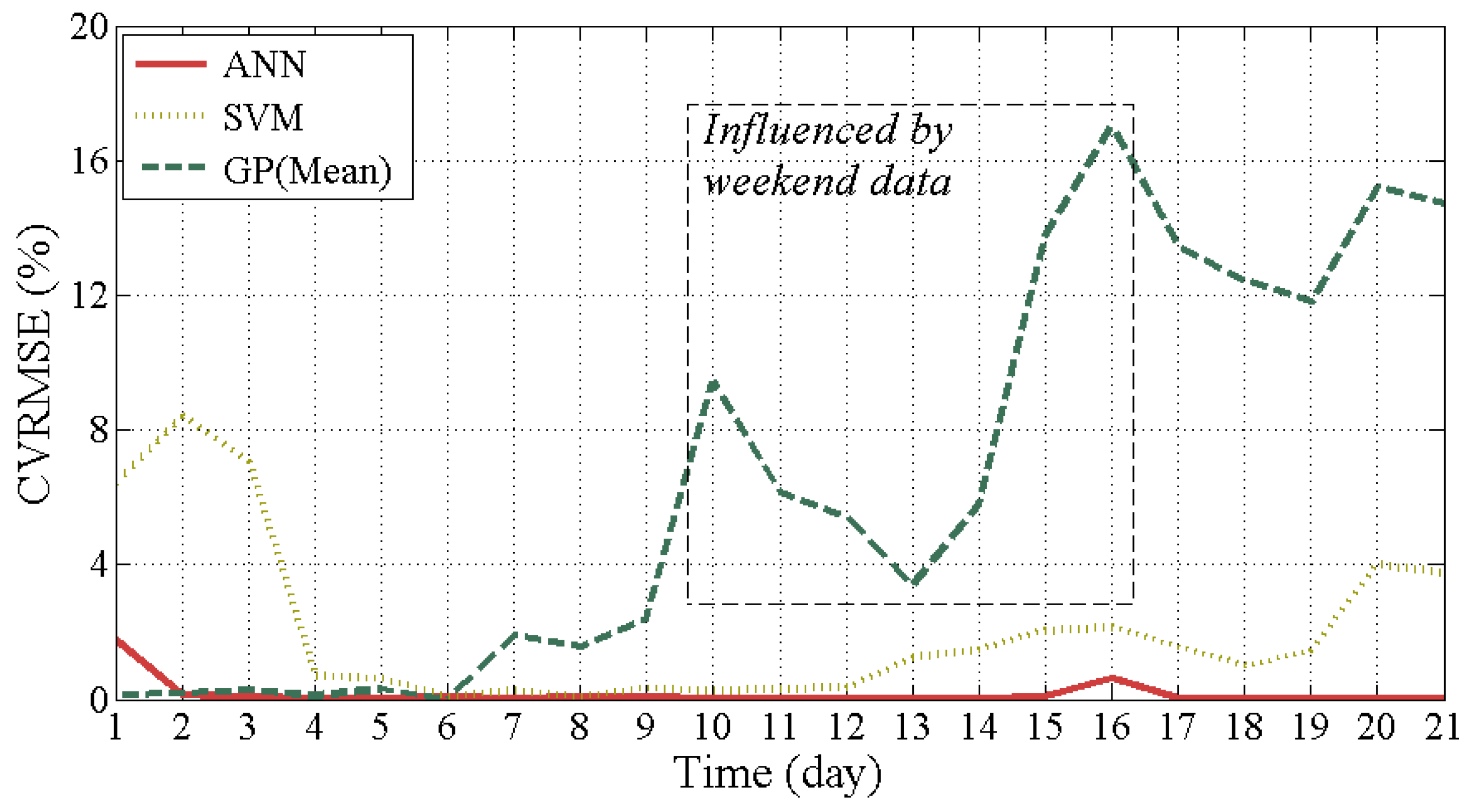
3.2. Issue #2: Training Period

In order to investigate the impact of the training period on the prediction accuracy of each model, the authors changed the training period from 1 day to 21 days (Figure 2). In this test, each of the aforementioned four inputs ($T_{out}$, $O$, $\Delta T_{chi},\text{ and }\Delta T_{cond}$) was entered in the model.

ANN (CVRMSE = 1.77%, MBE = 0.42%) and GP (CVRMSE = 0.13%, MBE = 0.06%) perform accurate prediction, even with a training period as short as one day (n = 288). However, SVM performs with less accuracy when the training period is less than four days (n = 1152). The SVM model performs satisfactorily when the training period is between four days and 12 days. If the training period is less than four days or greater than 12 days, its prediction accuracy decreases. In contrast, the ANN model shows consistent prediction accuracy regardless of the training period.

The GP model shows good agreement with the virtual measurement under a training period of less than seven days. However, the CVRMSE of the GP model increased when the training period was greater than nine days. This might be caused by the training data of the weekends (Days 6, 7, 8, and 9). In other words, it is inferred that the GP model might fail to perform prediction when an irregular data pattern such as weekdays vs. weekends exists in the training data set.

3.3. Issue #3–1: Selection of Inputs (Virtual Building)

The machine learning models are constructed based on a correlation between inputs and outputs; because of this, the inputs should be carefully selected. Inputs can be classified as endogenous and exogenous. The endogenous input is dependent on a building system and its control logic. The exogenous input is independent of the building system. In this study, the difference between return and supply chilled water temperatures (∆T_chi) and the difference between return and supply condensed water temperatures (∆T_con) are selected as endogenous inputs. Outdoor air temperature (T_out) and the number of occupants (O) are exogenous inputs.

Before attempting to use all four inputs, a correlation analysis was conducted in terms of the Pearson’s correlation coefficient. The coefficient, defined as Equation (14), identifies a correlation between the inputs and the output (the chiller’s energy demand).

$${\gamma }_{XY}={\displaystyle \sum }_{i=1}^n(x_i-\overline{x})\left(y_i-\overline{y}\right)/\sqrt{{\displaystyle {{\displaystyle \sum }}_{i=1}^n}{\left(x_i-\overline{x}\right)}^2{\left(y_i-\overline{y}\right)}^2}$$

(14)

where $\overline{x}\text{ and }\overline{y}$ are the mean of each X and Y. The correlation coefficients of the four inputs are shown in

Table 4. Correlation coefficient between inputs and output for the virtual building.

	Input (X)
	Tout	O	∆Tchi	∆Tcond
γXY 1	0.51	0.59	0.99	0.99

¹ Y (output): chiller’s electric demand.

. The endogenous inputs, ∆T_chi and ∆T_cond, are more influential on the output than the exogenous inputs, T_out and O. The coefficients of ∆T_chi and ∆T_cond are close to 1.0. In other words, they have a dominant effect on the chiller’s electric demand and are closely correlated to the output.

Table 5. Prediction with a different set of inputs.

	Inputs	RMSE (kW)	CVRMSE (%)	MBE (%)	Remark
ANN	Tout, O	71.9	74.2	−33.1	Exogenous inputs only
	∆Tchi, ∆Tcond	0.0008	0.0008	0.003	Endogenous inputs only
	Tout, O, ∆Tchi, ∆Tcond	0.103	0.105	0.054
SVM	Tout, O	65.3	67.4	−13.0	Exogenous inputs only
	∆Tchi, ∆Tcond	0.0007	0.0007	0.0003	Endogenous inputs only
	Tout, O, ∆Tchi, ∆Tcond	0.544	0.559	0.173
GP	Tout, O	115.1	118.9	100	Exogenous inputs only
	∆Tchi, ∆Tcond	0.0004	0.0004	0.0002	Endogenous inputs only
	Tout, O, ∆Tchi, ∆Tcond	0.943	0.922	0.337

shows that the models based on two endogenous inputs (∆T_chi, ∆T_cond) demonstrate the best performance. The exogenous inputs (T_out, O) are not informative for predicting the output. It is worth noting that the models with all four inputs underperform compared to the models with only two endogenous inputs. This signifies the importance of the careful choice of inputs for developing machine learning models.

The correlations shown in Table 4 were obtained for summer days (from 1 August to 7 August). The authors calculated the correlation coefficients of the four inputs over an entire year. Figure 3 shows that ∆T_chi and ∆T_cond have a strong correlation with the chiller’s energy demand over an entire year. The coefficient of ∆T_cond is close to 1.0 for the entire year. The coefficients of the endogenous inputs (T_out and O) are exchanged with each other around March and November. This implies that their correlation to the output could change due to the seasonal condition. In other words, the number of occupants is more influential to the chiller’s energy demand due to the heat generation of occupants. The outdoor air temperature is less correlated to the chiller’s energy demand during summer days since the building is an internal load-dominated office building.

4. Second Case Study: A Real-Life Building

In contrast to the first case study, the second case study was applied to the real-life building. The building is an office building located in Seoul, Korea (Figure 4). The building has five stories above ground and a single story underground. The cooling system includes two electric compression chillers and two cooling towers. The interior zones are served by nine VAV air handling units (AHUs) and the perimeter zones are conditioned by FCUs. The two chillers and cooling towers are connected in parallel to the AHUs and operated in turn depending on the building’s cooling requirement. The Building Energy Management System (BEMS) installed in this building saves measured data at a sampling time of five minutes. In a similar manner to the three models for the virtual building, the authors developed the data-driven models for the chiller’s energy demand of the existing building (Figure 4).

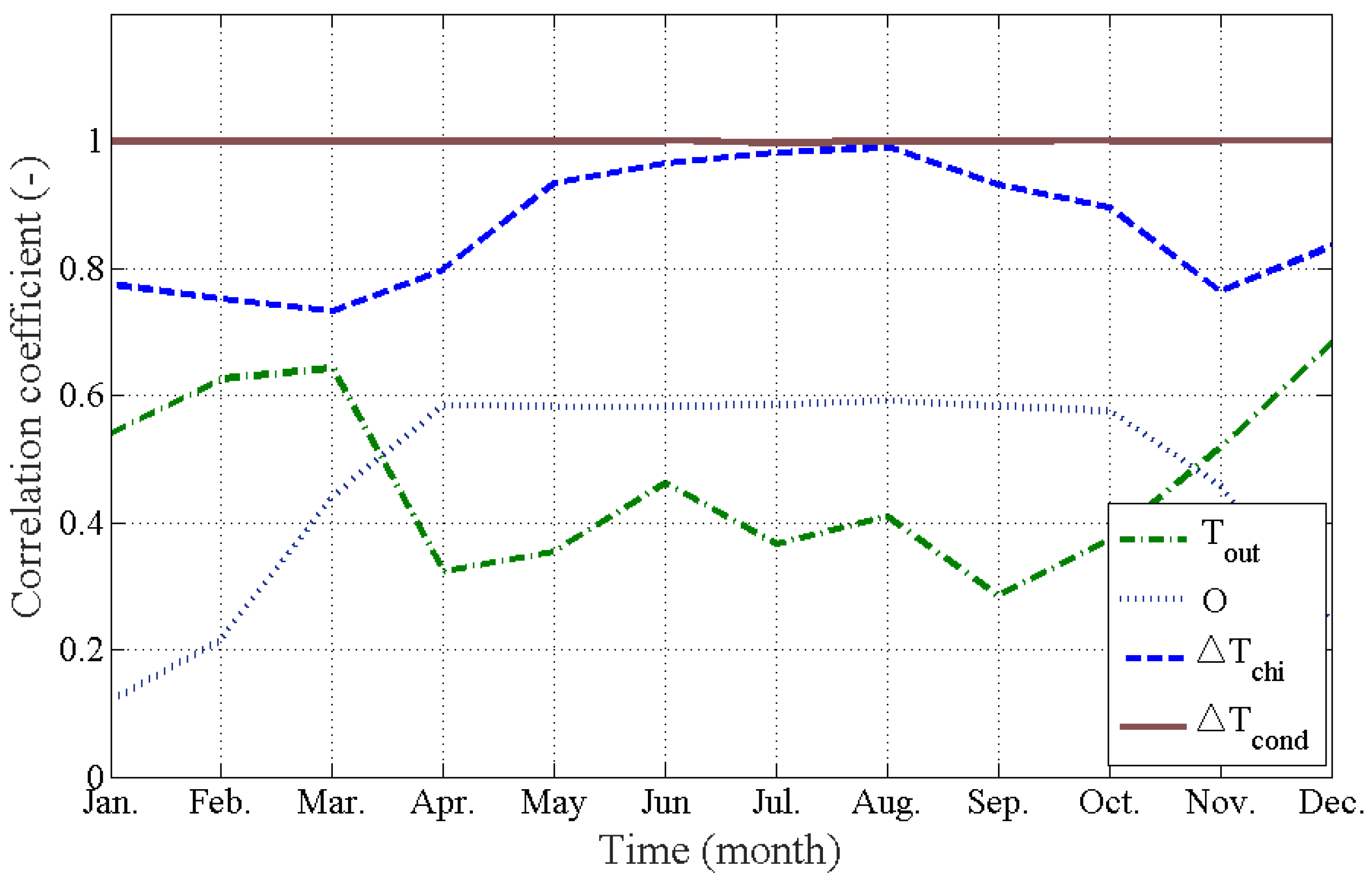
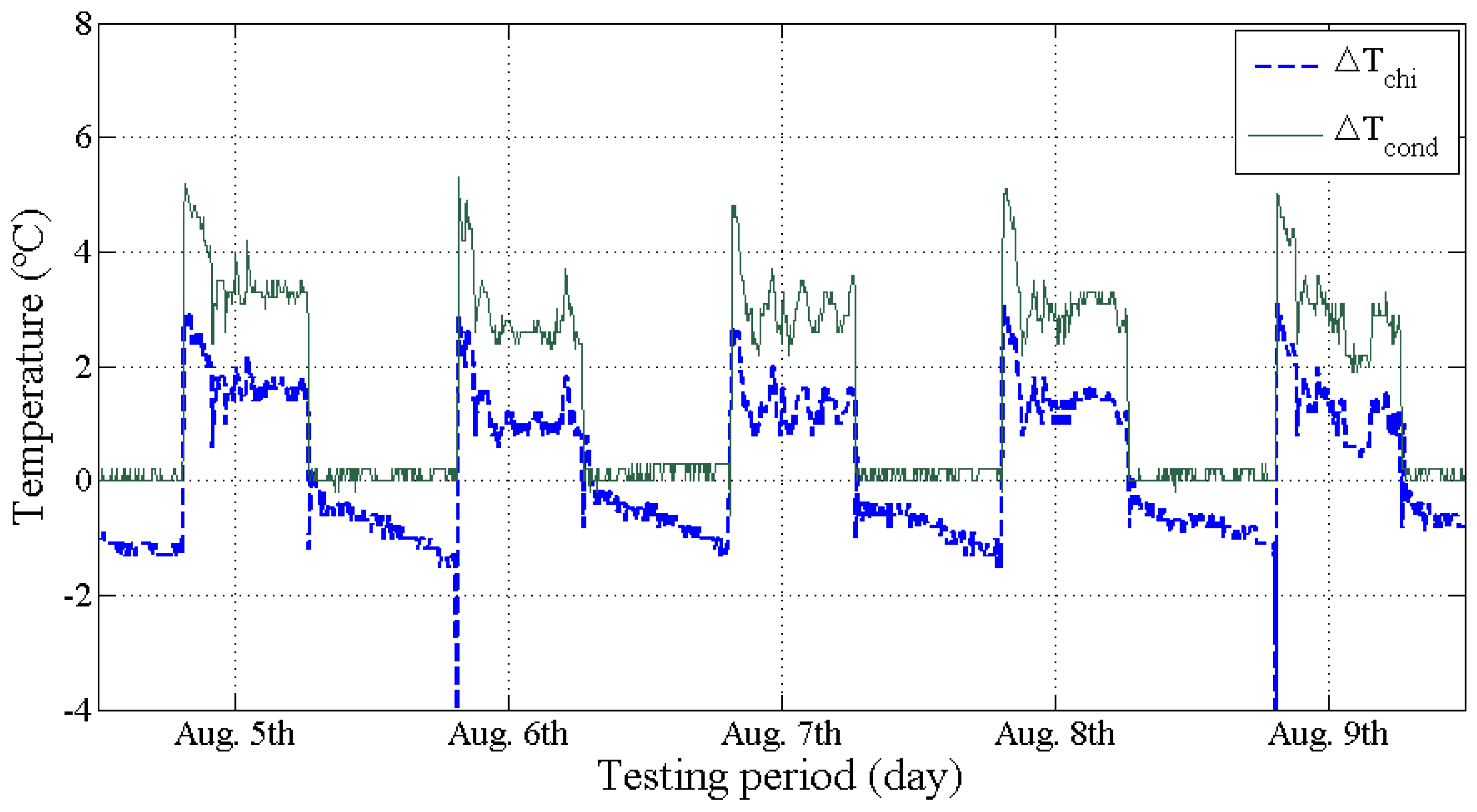
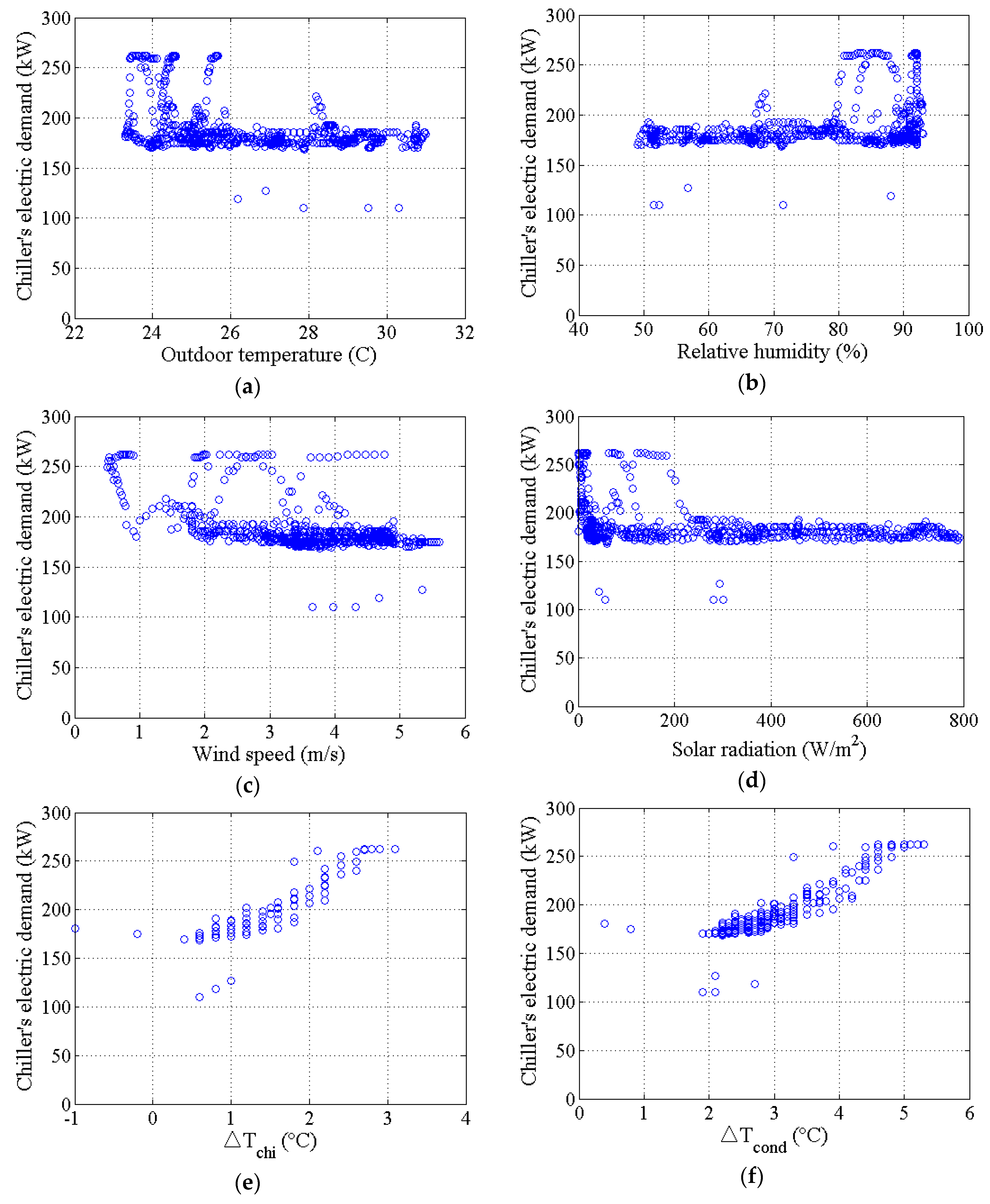
4.1. Issue #3–2: Selection of Inputs (Real-Life Building)

In other studies [6,7,19,20,21], weather inputs such as humidity, wind velocity, and solar radiation were used as exogenous inputs. Hence, the authors added more exogenous inputs (relative humidity (H_rel), wind speed (V_wind), and the sum of direct and diffuse solar radiation (ϕ)) to the three models.

This addition of exogenous inputs to the models was performed in order to investigate how the machine learning models of the chiller’s energy demand could be changed with new inputs included. The training period was set as seven days (29 July to 4 August). As seen in

Table 6. Correlation coefficients of exogenous inputs for the existing building.

	Input (X)
	Tout	Hrel	Vwind	ϕ
γXY 1	−0.38	−0.36	−0.52	−0.35

¹ Y (output): chiller’s electric demand.

and Figure 5, the correlations of weather inputs on the output are not as strong as those of ∆T_chi and ∆T_cond.

The data-driven models developed with the four exogenous inputs (outdoor temperature, relative humidity, wind speed, and solar radiation) cannot accurately capture the chiller’s hourly electric demand (

Table 7. Three models developed with only four exogenous inputs.

	RMSE (kW)	CVRMSE (%)	MBE (%)
ANN	50.45	25.51	6.17
SVM	90.96	46.00	2.29
GP	152.66	77.19	10.74

, Figure 6). It can be inferred that the weather inputs might influence the energy use of the entire building, but they cannot depict the chiller’s electric demand.

4.2. Issue #4: Missing or Outlying Data Obtained from BEMS

The measured data for the second case study contain missing or outlying data. The authors found 43 missing data points out of a total of 2016 data points (12 points per hour × 24 h per day × 7 days = 2016). With regard to the missing data, the authors applied a simple interpolation.

In addition, outlying data also exist due to sensor errors, noise, and the system’s malfunction. However, it is not easy to quantitatively discern outlying data. In this study, Random Sample Consensus (RANSAC) was employed in order to automatically detect and treat the outliers. RANSAC was performed as follows [22]:

• Hypothesize: Minimal Sample Sets (MSSs) are randomly selected from the input dataset and parameters of the RANSAC algorithm are computed using the elements of the MSS.
• Test: RANSAC checks the elements (also called “Consensus Set”, CS) of the entire dataset that are consistent. If the probability of finding a better ranked CS drops below a certain threshold, the RANSAC terminates.

As a result, the authors identify 123 outliers as shown in Figure 7. The performance of the machine learning models is significantly influenced by the training data. Hence, these outliers should be adequately treated. The outliers can be caused by malfunction of building systems or sensor errors (disturbance in the voltage or current of the measuring devices).

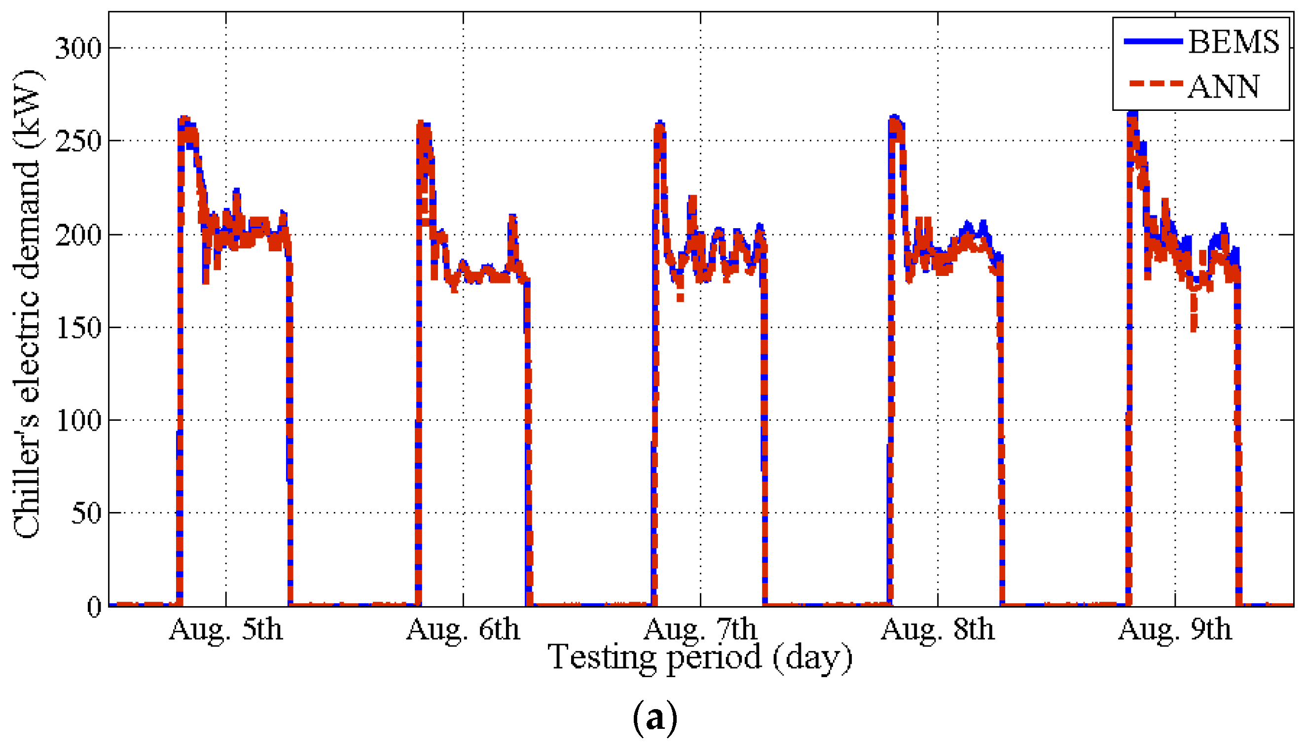
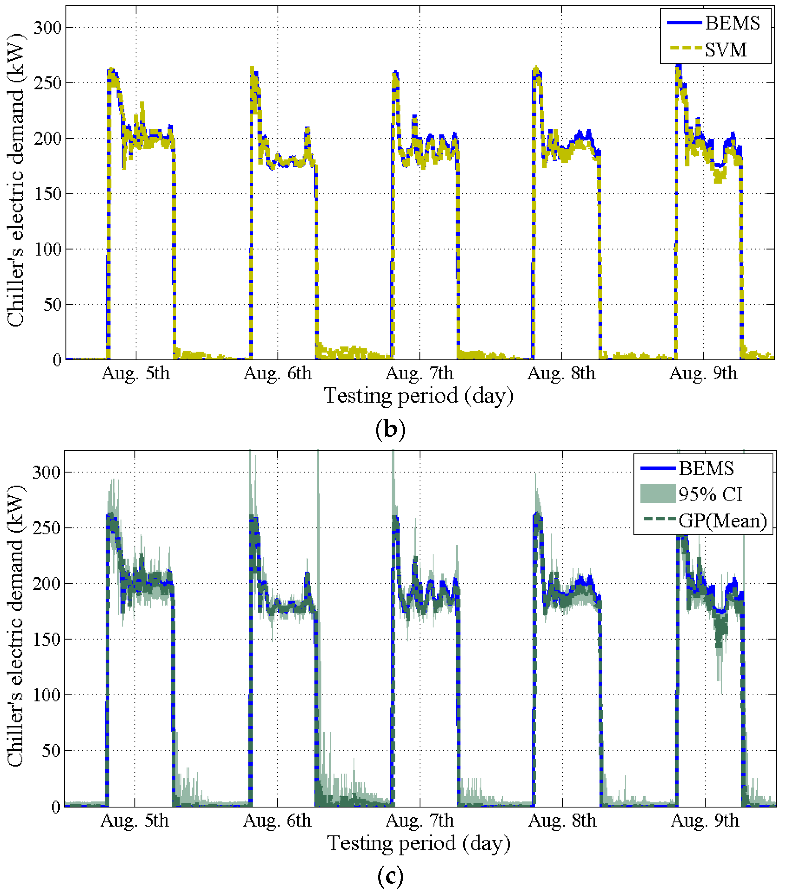
4.3. Issue#5: Validation of the Models

The authors tested the predictive performance of the three machine learning models during the summer period (5–9 August). The difference between return and supply chilled water temperatures (∆T_chi) and the difference between return and supply condensed water temperatures (∆T_cond) were selected as inputs, since they have strong correlation with the chiller’s electric demand (Table 5). During the training, the following inequality constraints were applied: the Coefficient of Variation of the Root Mean Square (CVRMSE) must be less than 15% and the Mean Biased Error (MBE) must be less than 5%.

The training periods of the three models were set as seven days (from 29 July to 4 August, 2016 points) and the testing periods were set as five days (from 5 August to 9 August, 1440 points). The sampling time was set at 5 min. Figure 8 shows the inputs during the testing period.

As shown in

Table 8. Prediction of the models.

	RMSE (kW)	CVRMSE (%)	MBE (%)
ANN	9.6	10.5	2.2
SVM	10.2	11.2	0.8
GP	10.0	11.0	1.4

and Figure 9, the prediction capability of all three models is surprisingly excellent. Compared to Table 4, the values of CVRMSE and MBE were increased since these models were tested not in the virtual case, but in the real-life case. The following points are important in this regard:

• The SVM model is the least effective in terms of computation time. The training took about 1 h with over 2160 data points. The computer used was an Intel(R) Core(TM) i5 CPU 2.8 GHz, RAM 6 GB, Windows 7, 64 bit.
• The ANN model shows better performance than the two other models, regardless of the training period (issues #2 and #3). However, the ANN model requires heuristic (trial and error) judgment to determine the number of hidden layers and nodes.
• The GP model could provide stochastic prediction with a confidence interval. However, the accuracy of the GP model significantly decreases when an irregular pattern of the data is included (issue #2).

5. Conclusions

The objective of this study was to compare the three most popular machine learning models (ANN, SVM, and GP). The three models were successfully developed to predict the electric demand of the chiller in a virtual building and a real-life building. If a prediction model of a chiller’s electric demand was developed using a first principles based model, it would require significant time and effort and engineering assumptions, in-depth knowledge of the system’s physics, and dynamic interaction between the chiller and the entire building, etc. Rather than resorting to a first principles-based model, this study demonstrated a straightforward and practical approach to developing a simulation model of a building system of interest using machine learning algorithms.

All three machine learning models have similar predictive qualities and showed good agreement with the virtual and real measurements. However, various important issues need to be considered as follows: reproducibility, selection of inputs, training period, and outlying data obtained from BEMS. The following issues need to be carefully taken into account:

• Remember that the data-driven model generated from a machine learning algorithm is not reproducible (issue #1).
• Determine the training period carefully. The GP model is strongly influenced by the training period. The ANN is least influenced by the training period (issue #2).
• Check the correlation between inputs and outputs (e.g., the Pearson’s correlation coefficient greater than 0.8) (issue #3).
• Be aware that the BEMS data from the real-life building include missing or outlying data. Such missing or outlying data could influence the prediction performance of the machine learning model (issue #4).
• Apply constraints during the training when needed (e.g., CVRMSE less than 15%, MBE less than 5%) (issue #5).

References

1. Ahn, K.U.; Kim, Y.J.; Kim, D.W.; Yoon, S.H.; Park, C.S. Difficulties and Issues in Simulation of a High-rise Office Building. In Proceedings of the 13th Conference of International Building Performance Simulation Association, Chambery, France, 26–28 August 2013; pp. 671–678.
2. Yang, J.; Rivard, H.; Zmeureanu, R. On-line Building Energy Prediction using Adaptive Artificial Neural Networks. Energy Build. 2005, 37, 1250–1259. [Google Scholar] [CrossRef]
3. Cam, L.M.; Zmeureanu, R.; Daoud, A. Comparison of Inverse Models used or the Forecast of the Electric Demand of Chillers. In Proceedings of the 13th International Building Performance Simulation Association, Chambery, France, 26–28 August 2013; pp. 2044–2051.
4. Dong, B.; Cao, C.; Lee, S.E. Applying support vector machines to predict building energy consumption in tropical region. Energy Build. 2005, 37, 545–553. [Google Scholar] [CrossRef]
5. Kim, Y.J.; Park, C.S. Nonlinear Predictive Control of Chiller System using Gaussian Process Model. In Proceedings of the 2nd Asia Conference of International Building Performance Simulation Association, Nagoya, Japan, 28–29 November 2014; pp. 594–601.
6. Heo, Y.S.; Zavala, V.M. Gaussian Process Modeling for Measurement and Verification of Building Energy Savings. Energy Build. 2012, 53, 7–18. [Google Scholar] [CrossRef]
7. Neto, A.H.; Fiorelli, F.A.S. Comparison between Detailed Model Simulation and Artificial Neural Network or Forecasting Building Energy Consumption. Energy Build. 2008, 40, 2169–2176. [Google Scholar] [CrossRef]
8. Ben-Nakhi, A.E.; Mahmoud, M.A. Cooling load prediction for buildings using general regression neural networks. Energy Convers. Manag. 2004, 45, 2127–2141. [Google Scholar] [CrossRef]
9. Amjady, N. Short-term hourly load forecasting using time-series modeling with peak load estimation capability. IEEE Trans. Power Syst. 2001, 16, 498–555. [Google Scholar] [CrossRef]
10. Kalogirou, S.A.; Bojic, M. Artificial neural networks for the prediction of the energy consumption of a passive solar building. Energy 2000, 25, 479–491. [Google Scholar] [CrossRef]
11. Wiliamowski, B.M.; Yu, H. Improved Computation for Levenberg–Marquardt Training, Neural Networks. IEEE Trans. Neural Netw. 2010, 21, 930–937. [Google Scholar] [CrossRef] [PubMed]
12. Han, J.; Kamber, M. Data Mining: Concepts and Techniques; Morgan Kaufmann: San Francisco, CA, USA, 2001. [Google Scholar]
13. Smola, A.J.; Scholkopf, B. A Tutorial on support Vector Regression. Stat. Comput. 2004, 14, 199–222. [Google Scholar] [CrossRef]
14. Wang, H.; Hu, D. Comparison of SVM and LS-SVM for Regression. In Proceedings of the International Conference on Neural Networks and Brain, Beijing, China, 13–15 October 2005; pp. 279–283.
15. Suykens, J.A.K. Nonlinear Modelling and Support Vector Machines. In Proceedings of the 18th IEEE Instrumentation and Measurement Technology Conference, Budapest, Hungary, 21–23 May 2001; pp. 287–294.
16. Roberts, S.; Osborne, M.; Ebden, M.; Reece, S.; Gibson, N.; Algrain, V. Gaussian Process for Time-series Modelling. Philos. Trans. R. Soc. A 1984, 371. [Google Scholar] [CrossRef]
17. Rasmussen, C.E.; Williams, C.K.I. Gaussian Process for Machine Learning; MIT Press: Cambridge, MA, USA, 2006. [Google Scholar]
18. Cormen, T.H.; Leiserson, C.E.; Rivest, R.L.; Stein, C. Introduction to Algorithms; MIT Press: Cambridge, MA, USA, 2001. [Google Scholar]
19. Zhang, Y.; O’Neil, Z.; Wagner, T.; Augenbroe, G. An Inverse Model with Uncertainty Quantification to Estimate the Energy Performance of an Office Building. In Proceedings of the 13th International Building Performance Simulation Association, Chambery, France, 26–28 August 2013; pp. 614–621.
20. ASHRAE. ASHRE Handbook-Fundamentals; American Society of Heating, Refrigerating, and Air-Conditioning Engineers, Inc.: Atlanta, GA, USA, 2013. [Google Scholar]
21. ASHRAE. ASHRAE Guideline 14: Measurement of Energy and Demand Savings; American Society of Heating, Refrigerating, and Air-Conditioning Engineers, Inc.: Atlanta, GA, USA, 2002. [Google Scholar]
22. Zuliani, M. RANSAC for Dummies; Vision Research Lab, University of California: Santa Barbara, CA, USA, 2009. [Google Scholar]
Figure 1. Target building for the 1st case study (simulation model of a virtual building).
Sustainability 08 00543 g001
Figure 2. Models’ prediction accuracy with regard to the training period.
Sustainability 08 00543 g002
Figure 3. Correlation coefficients over one year.
Sustainability 08 00543 g003
Figure 4. Target building for the second case study.
Sustainability 08 00543 g004
Figure 5. Chiller’s energy demand vs. exogenous and endogenous inputs: (ad) are exogenous and (ef) are endogenous inputs.
Sustainability 08 00543 g005
Figure 6. Measured and predicted chiller’s electric demand with only four exogenous inputs: (a) Artificial neural network; (b) Support vector machine; and (c) Gaussian process.
Sustainability 08 00543 g006
Figure 7. Result of Random Sample Consensus (RANSAC).
Sustainability 08 00543 g007
Figure 8. Inputs (∆Tchi and ∆Tcond) during the testing period.
Sustainability 08 00543 g008
Figure 9. Prediction of the three machine learning models: (a) Artificial neural network; (b) Support vector machine; and (c) Gaussian process with Confidence Interval (CI). BEMS: Building Energy Management System.
Sustainability 08 00543 g009aSustainability 08 00543 g009b