GHG Emissions, Economic Growth and Urbanization: A Spatial Approach

Abstract

To gain a greater understanding of the spatial spillover effect of greenhouse gas emissions and their influencing factors, this paper provides a spatial analysis of four gas pollutants (CO₂ emissions, SO₂ emissions, NO_x emissions, and dust emissions). Focusing on China, the paper also explores whether the four gas pollutants are influenced by the emissions of neighboring regions and other possible sources. The paper uses a global spatial autocorrelation analysis, local spatial association analysis and spatial lag model for empirical work. The results suggest that CO₂, SO₂, and NO_x emissions show significant positive results for both the spatial correlation and space cluster effect in provincial space distribution.CO₂ and NO_x emissions have a significant positive spillover effect, while the SO₂ emissions’ spatial spillover effect is positive but not significant. Economic growth and urbanization are the key determinants of CO₂, dust, and NO_x emissions, while energy efficiency and industrialization do not appear to play a role. This raises questions about the method of examining the spatial relationship between gas pollution, economic growth and urbanization in the future.

1. Introduction

Social production and living are becoming increasingly dependent on the use of natural resources. Greenhouse gas emissions (GHG_S) are of concern due to their adverse effects on global climate change and human sustainable development. The use of natural resources accelerates the production of greenhouse gas emissions, including CO₂ (carbon dioxide emission), NO_x (nitrogen oxide emission), SO₂ (sulfur dioxide emission) and dust emissions, which affect the balanced development of regional economies and the sustainable use of natural resources. Cities are the social center of human life and consumption and have become the primary source of energy consumption and greenhouse gas emissions. Greenhouse gas emitted from cities account for 70% of the world’s greenhouse gas emissions [1]. As governments and the general public have become more aware of environment protection issues in urbanization, greenhouse gas emissions have become the focus of the world’s attention [2]. Accordingly, GHGs spatial distribution in periods of economic growth and urbanization has become a compelling topic in the field of environment management and economics.

With rapid economic development and urbanization under carbon reduction target by 2020, China faces the threat of not only traditional carbon dioxide pollutants but also emerging SO₂, NO_x and dust emissions. However, on the whole, the focus on China’s emerging SO₂, NO_x and dust emission regional spatial analysis is rather limited. The existing studies on China’s regional emissions mostly focus on CO₂ emissions. Few studies have examined the aforementioned types of GHGs from a provincial perspective. In terms of methodology, few studies have conducted a spatial correlation.

China is suffering from air pollution and is becoming the center of the increasing concerns regarding GHG emissions; therefore, this study aims to address the regional disparity and discuss implications. This paper analyzes the regional GHG emissions pattern and correlated effects for policy decision. The policy implications would improve the efficiency of the policy implementation.

With the above background, this empirically-grounded study examines the relationship between economic factors and air pollutants (CO₂, SO₂, NO_x and dust) through a space analysis and further discusses the regional disparity and effects. In this paper, we introduce a spatial vector to the GHG emissions ordinary least squares estimation model and compare the errors and predicting accuracy of the two models. The objective of this study is to find an approach with the spatial factor and provide applicable policy meanings by considering the spatial correlations.

The research in this paper is structured as follows. First, this paper examines CO₂, SO₂, NO_x, and dust spatial relationships by employing a global spatial autocorrelation method using Moran’s I index to find whether the four gas emissions are positive correlated with the neighboring province’s emissions. Additionally, a local indicator of spatial association (LISA) method is used to examine the GHGs’ clustering effect. Finally, based on the above test, the first model is the ordinary least squares estimation model, and the second model is the spatial lag model, which was developed by adding the spatial dimension. We compare the four gas pollutants emissions determinants, which significantly affect the CO₂, SO₂, NO_x emissions and dust in a spatially correlated condition.

The remainder of the paper is structured as follows: Section 2 provides a theoretical background and suggests hypotheses; Section 3 discusses the model for the spatial econometric methodology and data; Section 4 discusses the data; Section 5 provides results, and Section 6 concludes.

2. Literature Review and Hypothesis

A growing body of literature on economic growth and GHG emissions has examined the impact of the factors of economic development on GHGs, such as “pollution heaven,” “race to the bottom” and “Environmental Kuznets curve (EKC) theory and hypothesis.” Among the possible economic development factors, the environmental Kuznets curve has become the mainstream method and is used in the current study. Grossman (1991) used an inverted U-curve EKC to describe the relationship between environmental quality and per capita income. Selden and Song (1994) found that four types of pollutants (suspended particulate matter, sulfur dioxide, nitrogen oxide and carbon monoxide) and per capita GDP had an inverted U-curve relationship [3]. Roberts and Grimes (1997) found there is an inverted U-shaped relationship between CO₂ emission intensity and economic growth [4]. Dinda (2005) and Verbeke (2006) examined the homogeneity of the EKC hypothesis [5,6]. Meanwhile, studies (M, Wagner, 2008) on the EKC heterogeneity of different regions and different pollutants were conducted [7]. A weakness of this part of the literature has always been the binary link between GHGs and economic growth or urbanization in time series approach. A smaller body of literature has therefore attempted to examine the spatial distribution of GHG emissions, mostly focusing on pollution from CO₂ emissions [8,9].

Regarding the research on urbanization and GHG emissions, most studies are based on the theory of the urbanization logistic curve, and one of the most important methods is the Northam’s type curve [10]. There are three types of influential frameworks used to examine the impact of the urbanization level on greenhouse gas emissions: direct causality, indirect causal relationship, and regulation of causality [11]. In the indirect impact framework, urbanization affects population migration, and population migration affects carbon emissions. Urbanization development causes population migration and changes the industrial structure, lifestyle and population spatial distribution [12]; the heat island effect is an example.

In the empirical research, many scholars [13] adopted the Granger causality test and time series method, which focuses on the VCR model, ECM model and STIRPAT to examine the relationship between urbanization and GHGs [14,15]. Most of the studies show that urbanization level had a positive impact on greenhouse gas emissions [14,16]. Some studies found no significance [17], but others showed a more complex relationship: the development of urbanization promoting the optimal allocation of energy resources and agglomeration effects to reduce greenhouse gas emissions [18]. Other research proves the existence of urbanization with the environmental Kuznets curve as an inverted U-shaped curve [14,19].

With the classic emission model, Kaya (1990) established an equation identifying the relationship between human economics, social activities and greenhouse gas emissions [20]. This equation, based on factorization methods, decomposed carbon emissions into four factors affecting greenhouse gas emissions: energy efficiency, energy intensity, economic development and population. The existing research on greenhouse gas emissions are mostly developed on the basis of the Kaya equation.

The above study did not consider the spatial relationship of greenhouse gas emissions. In the regional economic system, the environmental performance of a region is affected not only by the internal economic development but also by greenhouse gas emissions in the surrounding area in the presence of economic growth and urbanization. At the micro level, Maddison (2006)’s research on the basis of spatial lag and the spatial error model introduced the adjacent area’s variables to examine the effects of economic growth on pollutant emissions, and the results proved that one country’s pollutants are actually affected by the influence of the neighboring countries [21]. Albu (2007) also proved the above conclusion in the spatial distribution of European space [22]. Later, the classical OLS, spatial error and spatial lag models were used to prove that the United States sample does not support the EKC curve relationship, where the spatial lag model is optimal [23]. Wang (2013) used a spatial econometric analysis to prove that the environmental indicators of the local area are affected by other regions [24]. Cirilli (2014), on the basis of the spatial analysis of Italian samples, proved the spatial correlation of city development and carbon emissions [25]. At the micro level, Cole (2013) found that Japanese companies were affected by adjacent enterprise carbon emissions, reflecting the spatial correlation [26].

Spatial approaches of GHGS analysis have been used to analyze the spatial effects of GHGs, particularly CO₂ emissions. Dong, L et al. (2014) conducted a spatial analysis of SO₂, NO_x, and PM2.5 emissions. The results suggest that there was an evident cluster effect for CO₂ emissions [27]. Ma, J. J. et al. (2009) investigated the CO₂ emission levels of 30 provinces in China from 2000 to 2006 [28]. Chuai, X. W. et al. (2012) analyzed the spatial autocorrelation of carbon emissions and the spatial regression analysis between carbon emissions and their influencing factors. The spatial regression results show that the carbon GDP and population were the two main factors that had strengthened the spatial autocorrelation of carbon emissions [29]. Tang, Z. et al. (2013) estimate the amount of carbon dioxide emissions and its spatial variation in the tourism sector. The results show that the carbon dioxide emissions from tourist accommodations in coastal areas are generally greater than those in inland areas [30]. Videras, J. (2014) explored the relationship between emissions of carbon dioxide with population, affluence, and technology. The results show strong evidence of spatial heterogeneity [31]. Liu, Y. et al. (2014) applied the Durbin model and Regression on Population, Affluence and Technology (STIRPAT) model and found the spatial relationship between emissions and the all factors except energy prices [32]. Zhao, X. T. et al. (2014) investigated the influential factors of carbon dioxide emission intensity. The results suggest that energy prices have no effect on emission intensity; per-capita, province-level GDP and population density had a negative effect on CO₂ emission intensity; energy consumption and the transportation sector had a positive effect on CO₂ emission intensity [33]. We give a literature summary of the factors in

Table 1. Comparison of Spatial Approach and Factors.

Authors	GHGs Type	Methods	Significant Factors	Not Significant Factors
Albu, L. L. (2007)	CO2	Three-Dimensional Map;	Influence Economic Growth	-
Ma, J. J. et al. (2009)	CO2	Spatial Autoregressive Models	Energy Intensity; Economic Development; Population Growth	Urbanization is not inevitable
Chuai, X. W. et al. (2012)	Carbon	Spatial Autocorrelation; Spatial Regression	GDP; Population	-
Cole, M. A. et al. (2013)	Carbon	OLS; Spatial Error Model	Size; Capital-Labor Ratio; R&D Expenditure; Exports; Concern	-
Dong, L. (2014)	SO2; NOx; PM2.5; CO2	Spatial Auto-Correlation; Multi-Regression Model	Population; GDP; Energy Consumption	Energy- Intensity
Zhao, X. T. et al. (2014)	CO2 Intensity	Spatial Panel Data Models	GDP; Population Density(Negative); Energy Consumption(Positive)	Energy Prices
Liu, Y. et al. (2014)	Carbon	Spatial Durbin Panel Model;	Population, Urbanization, Economic Development, Energy Intensity, Industrial Structure, Energy Consumption Structure, Openness	Energy Prices
Videras, J. (2014)	Carbon	Geographical Weighted- Regression	Spatial Heterogeneity	-
Kang, Y. Q. et al. (2016)	CO2	Spatial Panel Data Model;	Urbanization, Coal Combustion, Economic Growth	Trade Openness

.

Therefore, we propose the following hypotheses:

Hypothesis 1: 

Regional greenhouse gas emissions are spatial correlated and clustered.

Hypothesis 2: 

Urbanization and economic growth have a positive effect on greenhouse gas emissions.

Hypothesis 3: 

Regional greenhouse gas emissions have a spatial spillover effect.

To summarize, there are some gaps in the study on greenhouse gas emissions: first, many studies focus on the macro level or a specific industry, while research at the regional level is limited. Second, existing models cannot better reflect the spatial relationship of a spatial reaction between regions. For example, using time series data to examine the relationship between regional economic growth and carbon emissions obviously cannot comprehensively reflect the spatial relationship between the provinces, and the Granger causality analysis cannot solve the endogeneity problem. Furthermore, the current research focuses on the two-dimensional relationship between the urbanization level, economic growth, industrialization and carbon emissions and pays little attention to comprehensive factors [17,34,35]. Although very few studies have conducted a spatial analysis of the four types of GHG_S, there have been several attempts to analyze CO₂ pollutants and their effects [29,36,37]. Nevertheless, despite the various types of modeling methodologies available and continuous refinement, all the numerical models suffered from an ignorance of spatial factors. To overcome these shortcomings, the trend of using a spatial approach seems to be increasing because they outperform the classical statistical approaches. Some approaches have been previously used for different purposes in some studies on gas pollutants, particularly in carbon emissions modeling.

Compared to the above research, this paper—based on the spatial model—uses a spatial econometrics analysis to examine the spatial relations between economic growth, urbanization, the level of industrialization, energy efficiency and greenhouse gas emissions.

3. Methods

3.1. Spatial Relationship Modeling

Spatial effect refers to the spatial interaction between regional economic and geographic behavior, including spatial heterogeneity and spatial autocorrelation. The spatial correlation is decided by absolute position and relative position. We mainly use the global spatial correlation test and local spatial correlation test to test the spatial effect of China’s regional greenhouse gas emissions.

Spatial weight matrix W reflects the spatial relationship in spatial econometrics. In this paper, the data samples are derived from the data of all provinces in China. Therefore, the spatial weight matrix is the queen spatial weights, as seen in Equation (1).

$$W=\left(\begin{array}{cccc}{w}_{11}& w_{12}& \cdots & w_{1n}\\ w_{21}& w_{22}& \cdots & w_{2n}\\ ⋮& ⋮& ⋮& ⋮\\ w_{m1}& w_{m2}& \cdots & w_{mn}\end{array}\right)$$

(1)

3.1.1. Global Spatial Autocorrelation Method

Global spatial auto correlation refers to the overall regional spatial characterization of the regional GHG emission space distribution of clusters. This paper uses Moran’s I index method to verify the global spatial correlation for GHG emissions. The global Moran’s I index is defined as follows:

$$Moran’sI=[{\displaystyle \sum _{i=1}^n{\displaystyle \sum _{j=1}^{n}wij(Yi-\overline{Y}}})]/[S^2{\displaystyle \sum _{i=1}^n{\displaystyle \sum _{j=1}^n{W}_{ij}}}]$$

(2)

$$S^2=1/n{\displaystyle \sum _{i=1}^n(Yi-\overline{Y)}}$$

(3)

$$\overline{Y}=1/n{\displaystyle \sum _{i=1}^n{Y}_i}$$

(4)

where Yi represents the observed value of region i (greenhouse gas emissions), n is the total number of provinces, and Wij represents distant space weight matrix. The global Moran’s I range from −1 to 1. If the observed value of each region is spatially positively correlated, Moran’s I is larger. If the observed value of each region is spatially negatively correlated, Moran’s I is smaller, which shows that the difference of the spatial unit is larger; if the index is 0, the space is subject to a random distribution.

We use the asymptotic normal distribution test for the Moran’s I index test, as shown in Equation (5):

$$Z(d)=\frac{Moran’sI-E(Moran’sI)}{\sqrt{VAR(Moran’sI)}}$$

(5)

3.1.2. Local Spatial Association Method

Local indicators of spatial association (LISA) are used to examine local spatial relationships. Anselin (1995) believed that local indicators of spatial association (LISA) could describe the spatial clustering effect between one spatial unit and the surrounding units at a certain significance level [38]. This paper uses the local Moran’s I index to analyze the local spatial correlation, as shown in Equation (6):

$$Mora{n}^{’}s I_i=Z_i{\displaystyle \sum }_{j=1}^n{w}_{ij}{Z}_j\left(i\ne j\right)$$

(6)

where i represent space unit i, Zi and Zj denote deviation, and Wij represents the space weight matrix.

3.2. Traditional GHG Emissions Model

Kaya (1990) decomposes GHG (CO₂) emissions into four factors related to human production and living to explain the relationship between human activity and greenhouse gas emissions. The Kaya equation is expressed as shown in Equation (7):

$$GHG=\frac{GHG}{TOE}\times \frac{TOE}{GDP}\times \frac{GDP}{POP}\times POP$$

(7)

where GHG denotes greenhouse gas emission, TOE denotes energy use, GDP denotes gross domestic product, and POP denotes population. The ratio of GHG to TOE represents greenhouse gas emission per unit of energy use, which indicates the ability to use clean energy and the energy structure of this region. The ratio of TOE to GDP is energy intensity (GHG emissions per unit of output), indicating the industrialization level. The ratio of GDP to POP represents GDP per capital, which indicates the economic growth. POP represents population, which indicates the quality of urbanization.

Based on the above Kaya equation, we can now consider GHG emissions in equilibrium, which is defined as:

$$GH{G}_i=f(E{E}_i,E{I}_i,P{G}_i,PO{P}_i,{\epsilon }_i)$$

(8)

where EE_i represents energy efficiency, EI_i represents energy intensity; PG_i represents GDP per capital, and U_i represents population. To rule out the heteroscedasticity problem, we adopt the natural logarithm for the variables in Equations (7) and (9):

$$LnGH{G}_i=ai+{\beta }_{1i}LnE{E}_i+{\beta }_{2i}LnE{I}_i+{\beta }_{3i}P{G}_i+{\beta }_{4i}PO{P}_i+{\epsilon }_i$$

(9)

where β_1i represents the elasticity coefficient of the energy consumption structure, β_2i represents the elastic coefficient of the industrialization level, β_3i represents the elastic coefficient of economic growth, and β_4i represents the elastic coefficient of the urbanization level.

3.3. Spatial GHG Emission Model

The above is a classic emission model, but the classic emission model ignores the spatial correlation. If the classical OLS estimation results show the regional greenhouse gas emissions and economic growth, the development of urbanization has a positive relationship. However, the index test proves that the classical regression error has a spatial correlation, which indicates the influence of geographical location on the regional environmental pollution index.

To consider the other regional greenhouse gas emissions spatial spillover effects, we establish the space lag model by adding the space dimension in Equation (10):

$$GH{G}_{it}=f(E{E}_{it},E{I}_{it},P{G}_{it},PO{P}_{it},OGH{G}_{it},{\epsilon }_{it})$$

(10)

$$OGHG={\displaystyle \sum _{j=1}^n{w}_{j}GHG{E}_j}$$

(11)

where n denotes the number of adjacent regions in the spatial weight matrix, Wij denotes the spatial weight, GHGEj is the GDP of the adjacent j region, and OGHG denotes the greenhouse gas emissions of adjacent regions.

4. Data

In this paper, carbon emissions are calculated based on the IPCC method according to the “IPCC national greenhouse gas inventory guide,” as seen in Equations (12) and (13):

$$CE={\displaystyle \sum _{i=1}^n{N}_i}\times {\mathsf{\delta }}_{\mathrm{i}}$$

(12)

$${\mathsf{\delta }}_{\mathrm{i}}=C\times CEF\times COR\times CCF$$

(13)

where CE represents the total carbon emissions, I denote the energy consumption type; N represents the total consumption of energy yi (10⁴ tons standard coal), δ_i represents the carbon emission coefficient, C represents the low calorific value, CEF represents the carbon emission factors, CO represents the carbon oxidation rate, and CCF represents the carbon conversion coefficient.

Data for other greenhouse gases, such as nitrogen oxides emissions (NO_x), sulfur dioxide emissions (SO₂) and dust emissions, are obtained from China’s Bureau of Statistics website. The regional GDP data and energy use data are from the China Energy Statistical Yearbook [39]. The gross domestic product (GDP) uses 1990 as the base year, and the unit is billion Yuan.

The spatial weight matrix is provided by the National Geographic Information System Web using Geoda software (Luc Anselin, Tempe, AZ, USA). The Moran’s I scatter plot is drawn by the spatial statistical analysis software Geoda [40].

5. Results and Discussions

5.1. Global Spatial Autocorrelation Test Results

The greenhouse gas emissions are reflected in the following spatial distribution characteristics. Overall, high greenhouse gas emissions areas are clustered in the coastal areas of China, such as the Bohai Sea area, the Pearl River Delta region, and the Yangtze River Delta region, which show spatial clustering characteristics.

Specifically, there are three high emission clusters: North (Hebei, Shandong, Henan, Liaoning, Inner Mongolia), East (Shanghai, Jiangsu, Zhejiang cluster) and South (Pearl River Delta).The mid-level emission clusters are North (Heilongjiang), South (Hunan, Hubei, Anhui), and Southwest (Sichuan, Guizhou).The lower emission clusters are Northwest (Tibet, Qinghai, Gansu, Ningxia), Southwest (Chongqing), Southeast (Jiangxi), and South (Hainan).

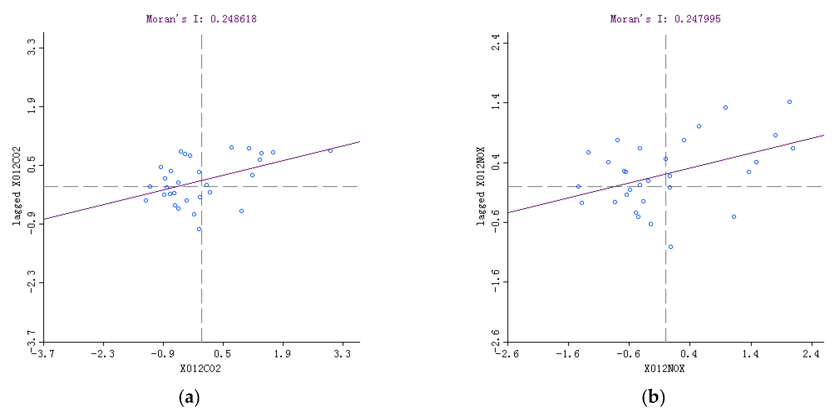
From the empirical results of

Table 2. The Moran’s I Statistics of China’s Greenhouse Gas Emissions.

GHGs	Moran’s I Statistics	P-Value	Expected Value	Mean	Standard Deviation	Z
CO2	0.3014	0.006 *	−0.0345	−0.0369	0.1081	3.1299
NOx	0.2903	0.004 *	−0.0345	−0.0354	0.1096	2.9637
SO2	0.1832	0.059	−0.0345	−0.0290	0.1210	1.7544
Dust	0.2227	0.014 *	−0.0345	−0.0354	0.1101	2.3457

Note: (1) Random test using the 9999permutation; (2) * 5% significance level.

, the global Moran’s I index of CO₂ emissions, NO_x emissions, SO₂ emissions, and dust emissions are 0.3014, 0.2903, 0.1832, and 0.2227, respectively. After the Monte Carlo simulation test, the Z values of all the above pollutants, except the SO₂ global Moran’s I index, are greater than 1.96, and their P values are less than 5%, which show significant positive spatial autocorrelation. This test result indicates that all GHGs, except SO₂ emissions, have spatial clustering characteristics and are geographically spatial auto-correlated, as shown in Table 2.

Figure 1 is a scatter diagram of the four types of GHG emissions. It can be seen that China’s provincial GHG emissions show spatial distribution characteristics in which CO₂ emissions, NO_x emissions, and dust emissions have a significant positive autocorrelation. Most of the points are located in Quadrant I and Quadrant II. These results are consistent with H1: The regional greenhouse gas emissions are spatially correlated except for SO₂ emission.

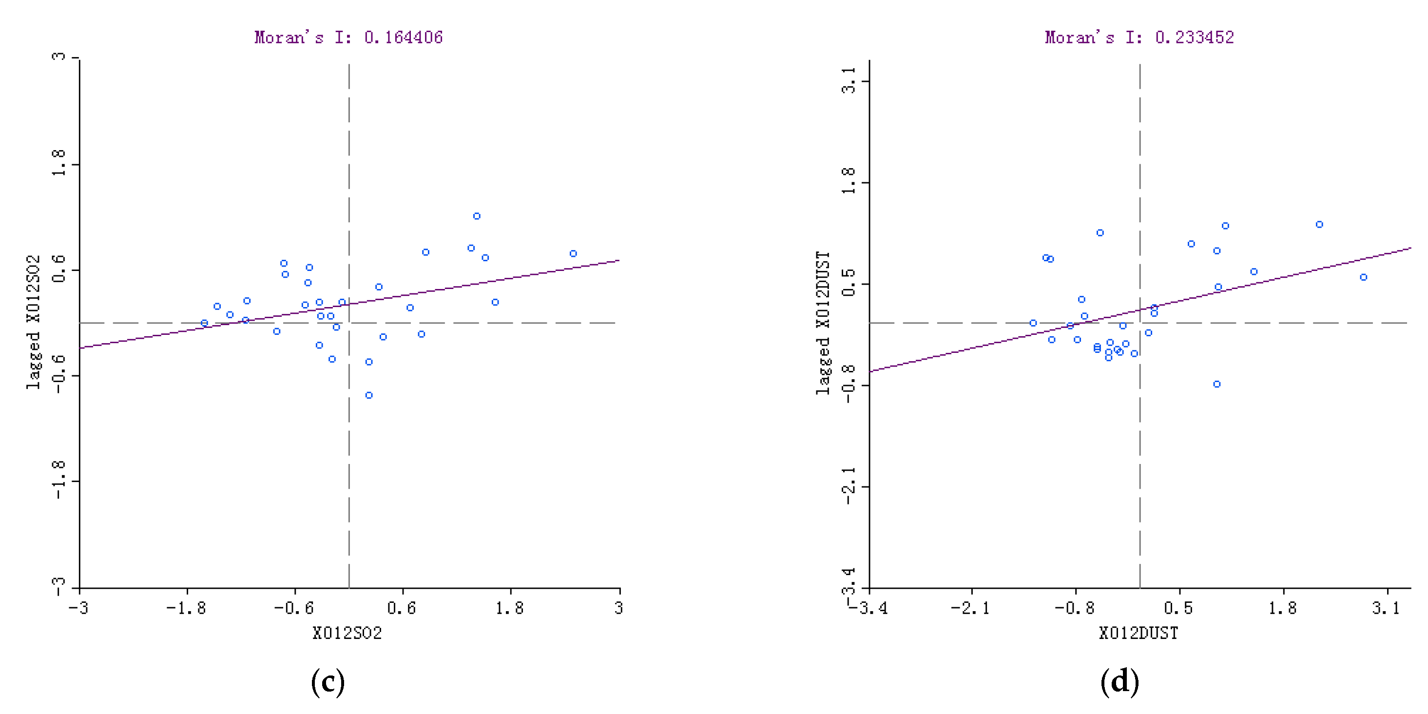
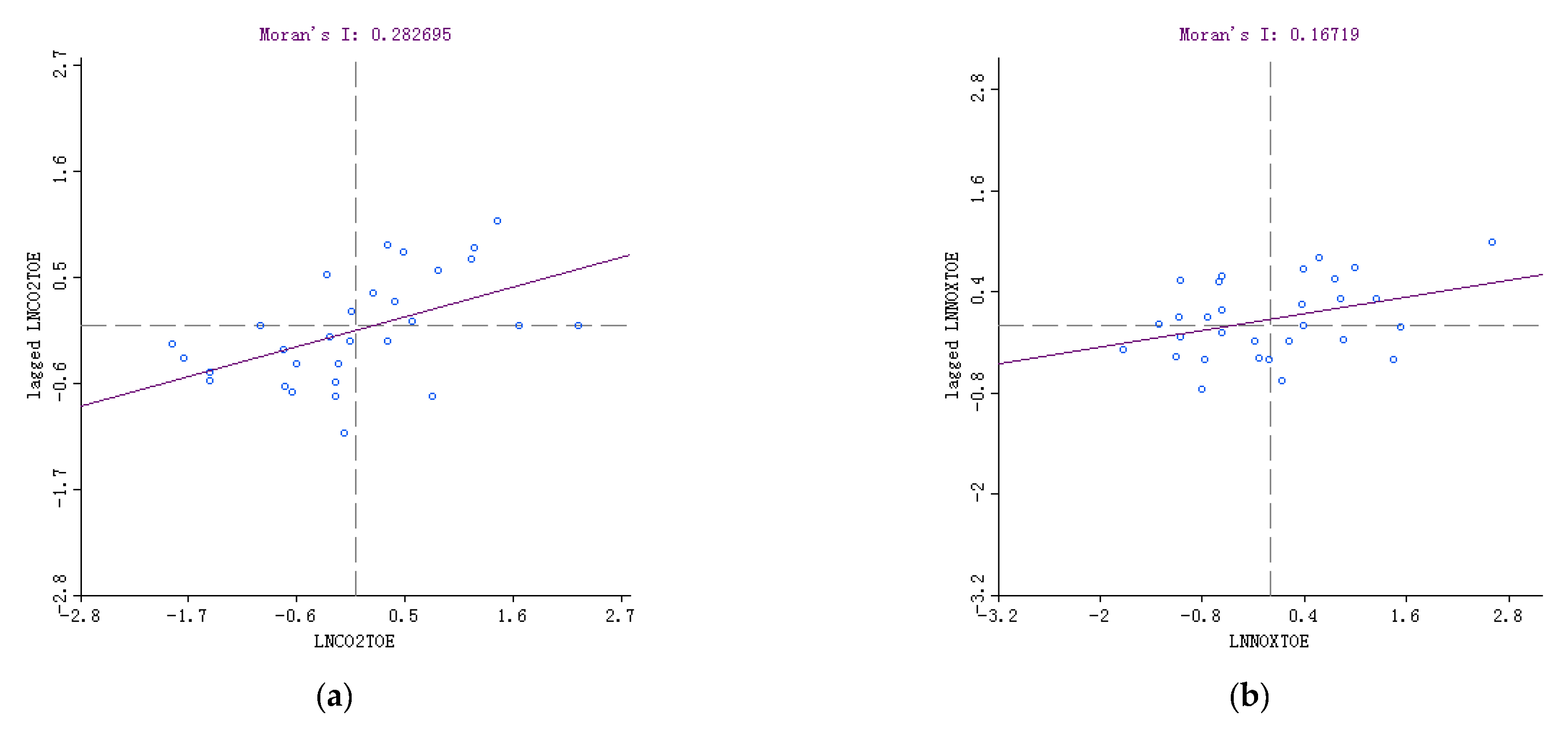
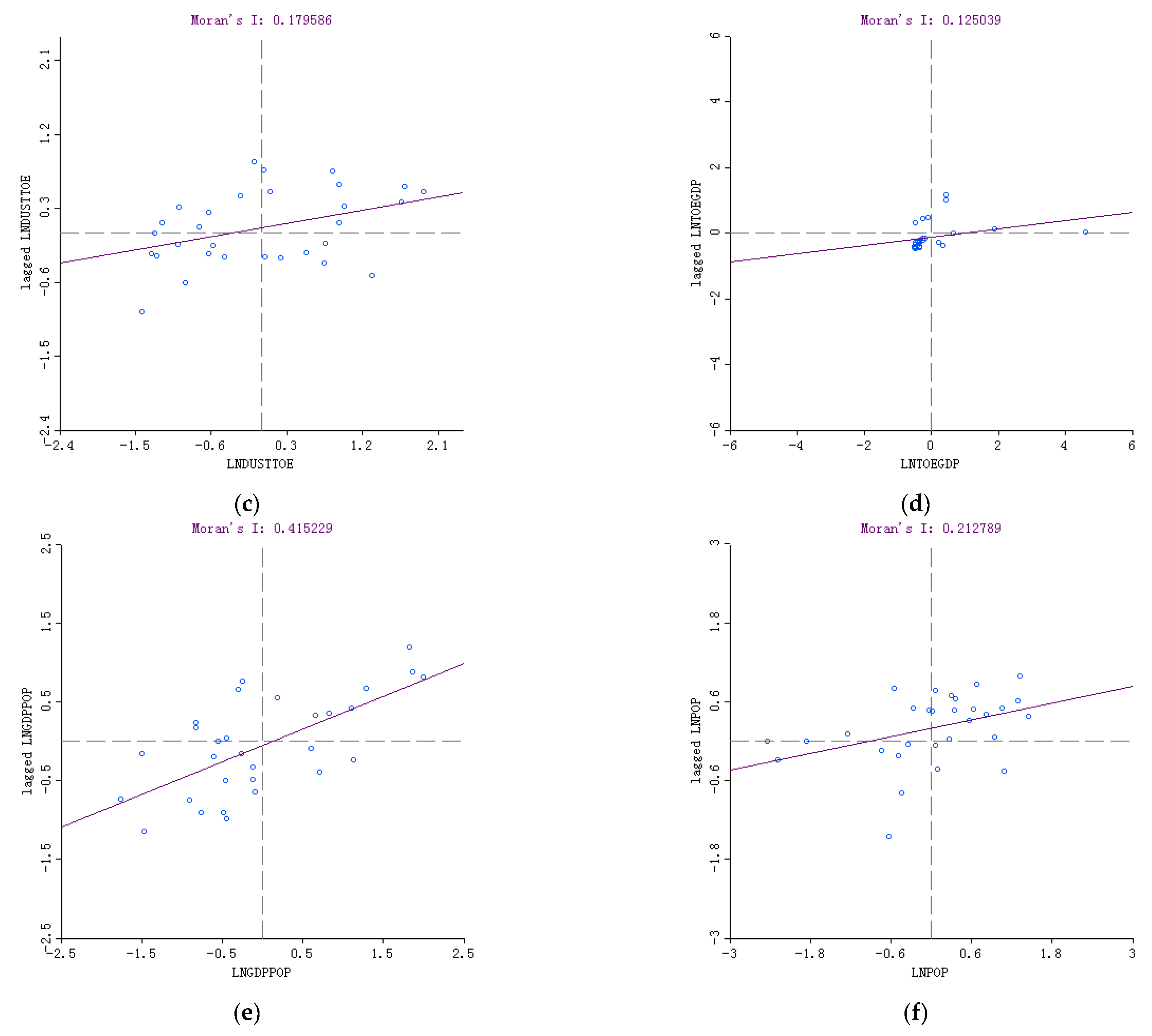
As

Table 3. The Moran’s I Statistics of gross domestic product (GDP), POP and Energy Efficiency.

Dependent Variables	Moran’s I Statistics	P-Value	Expected Value	Mean	Standard Deviation	Z
GDP	0.2599	0.018 *	−0.0345	−0.0260	0.1143	2.4663
TOE	0.1717	0.049 *	−0.0345	−0.0347	0.1128	1.8300
POP	0.2127	0.002 *	−0.0345	−0.0333	0.1152	2.4928
CO2EE	0.2827	0.004 *	−0.0345	−0.0309	0.1180	2.6577
NOxEE	0.1672	0.048 *	−0.0345	−0.0320	0.1097	1.7914
DUSTEE	0.1795	0.046 *	−0.0345	−0.0377	0.1207	1.8009
EI	0.1250	0.040 *	0.0345	−0.0348	0.0795	2.0103
PG	0.4152	0.001 *	−0.0345	−0.3500	0.1189	3.7870

Note: (1) Matrix random test using the 9999permutation; (2) * 5% significance level.

shows, Moran’s I index test of urbanization development, economic growth and the industrialization level and energy efficiency are significantly positive. These results show a positive spatial autocorrelation. Carbon dioxide (CO₂) and nitrogen oxide (NO_x) emissions are important indicators of the degree of environmental development, representing the environmental impact of economic activities’ frequency and intensity. As a result, there is a lag effect when GDP, population, energy consumption and energy efficiency result in the diffusion and transfer of greenhouse gas emissions between the provinces.

Figure 2 shows Moran’s I scatter plot of the other provincial factors, including GDP, population, energy efficiency and energy intensity. Most of the points are located in Quadrant I and Quadrant II, showing that the economic growth and urbanization of one region is spatially related.

5.2. Local Spatial Association Test Results

To examine the characteristics of the clustering effect, we use local indicators of spatial association (LISA) to evaluate the spatial patterns and characteristics of greenhouse gas emissions.

As seen in

Table 4. Local Spatial Association Pattern Classification of Moran’s I Plot.

Quadrant	Pattern	CO2	NOx	SO2	DUST
I	H-H	Hebei *, Henan *, Shandong *, Shanxi *	Hebei *, Henan *, Shandong *, Shanxi *, Anhui *	Hebei *, Henan *, Shandong *, Shanxi *, Anhui *	Inner Mongolia *, Liaoning *, Hebei *, Shanxi *, Shandong *, Henan *
II	L-H	Anhui *, Liaoning *			Jilin *
III	L-L	Xinjiang *, Sichuan *	Sichuan *
IV	H-L

Note: (1) Matrix random test using the 9999 permutation; (2) * 5% significance level.

, the results from CO₂ emissions LISA test show that Henan, Shanxi, Shandong, Anhui, and Sichuan pass the 5% significance level test, and Hebei is significant at 1%. Hebei, Henan, Shandong, and Shanxi are distributed in the first quadrant (H-H), showing a spatial distribution of the high carbon emissions region and a positive spatial correlation with the other provinces. Anhui is located in the second quadrant (L-H), showing that it is a low carbon province surrounded by high carbon emissions provinces. Sichuan and Xinjiang are located in the third quadrant (L-L) because they are low carbon emissions provinces with a negative spatial correlation with the other provinces.

The above results further prove Hypothesis 1: Regional greenhouse gas emissions show a spatial clustering effect.

5.3. Classical Spatial Weighting Method Evaluation

From the above spatial analysis, regional greenhouse gas emissions are shown to be widely affected other provinces, so this paper examines the spatial spillover effect of greenhouse gas emissions.

As in

Table 5. Spatial Weight of Ordinary Least Squares Estimation.

GHGS	EE	EI	PG	POP	R2	LMLAG	LMERR
CO2	1.0780 (0.0001 *)	1132.752 (0.0200 **)	0.6121 (0.0004 *)	0.9848 (0.0000 *)	0.8359	8.2622 (0.0041 **)	4.8055 (0.0284 **)
NOx	183.2002 (0.0003 *)	983.44 (0.0782 ***)	0.5643 (0.0024 **)	0.9786 (0.0000 *)	0.8205	4.0359 (0.0445 **)	4.0356 (0.0446 **)
SO2	268.95 (0.0000 *)	954.02 (0.1040)	0.7418 (0.0018 **)	1.0410 (0.0000 *)	0.8471	0.3868 (0.5340)	0.8638 (0.3528)
Dust	471.9864 (0.0000 *)	1180.69 (0.0201 **)	0.6505 (0.0008 *)	1.0862 (0.0000 *)	0.8952	6.8620 (0.0088 *)	0.7607 (0.3831)

Note: *, **, *** denotes 0.01, 0.05, 0.1 significance level.

, we use the classical spatial weighting method for the OLS estimation and find that the impact of economic growth, urbanization and other factors on CO₂, NO_x and dust emissions is significant at the 5% level. The results are consistent with H2: City development and economic growth have a positive effect on all four greenhouse gas emissions.

The ordinary least squares estimation showed that CO₂, NO_x, and dust emissions have close relationship with energy efficiency, energy intensity, GDP per capital and population.

The positive coefficient suggests that the influence of CO₂, NO_x, SO₂, and dust emissions based on energy efficiency energy intensity, GDP per capital and population is positive. The coefficient of GDP per capital and the four pollutants (CO₂, NO_x, SO₂, and dust) can describe the pull function for emissions by GDP. The results confirm Hypothesis 2: urbanization and economic growth have positive effects on greenhouse gas emissions.

The r-squared rate of the regression between dust and NO_x emissions GDP is higher than that of CO₂ emissions. This suggests that with the development of economic growth and carbon reduction policies, dust and NO_x are starting to play an important role in gas pollute composition.

5.4. Spatial Lag Model Evaluation

As seen in

Table 6. Coefficients of Spatial Lag Model Estimation.

Dependent Variables	W_GHGs	EE	EI	PG	POP	R2
CO2 emission	0.0881 (0.0015 *)	0.5222 (0.5317)	713.56 (0.0625 ***)	0.4822 (0.0001 *)	0.8422 (0.0000 *)	0.8788
NOx emission	0.1455 (0.0386 *)	10384.05 (0.0130 **)	73887.2 (0.1363)	43.52 (0.0076 *)	60.19 (0.0000 *)	0.6711
DUST emission	0.2469 (0.0021 *)	408.13 (0.0000 *)	875.20 (0.0248 **)	0.4392 (0.0039 **)	0.9212 (0.0000 *)	0.9217

Note: *, **, *** denotes 0.01, 0.05, 0.1 significance level.

, aside from the SO₂ emissions, the other three gas emissions’ LMLAG and LMERR statistical values are significant at the 5% level. The LMLAG test is more significant than the LMERR test, and the R-lMLAG test is more significant than the R-lMERR test. Thus, we could establish a spatial lag model of CO₂, NO_x and dust.

As seen in Table 6, the results show that the coefficients of economic growth, city development, industrialization, and energy intensity on carbon dioxide (CO₂) and nitrogen oxide (NO_x) pass the 10% level of significance test. The spatial correlation coefficient passes the 10% significance level test, showing that the provincial GHG emissions have a spillover effect, proving Hypothesis 3: regional greenhouse gas emissions have spatial spillover effects.

The contribution of GHG emissions from neighboring regions, population and economic growth to carbon emissions increased, but the contribution of energy intensity decreased. The carbon emissions spillover effect was aggravated due to the increase of economic growth and urbanization; thus, economic growth and urbanization were the two main factors that had strengthened the spatial autocorrelation of carbon emissions.

5.5. Comparison of Spatial Weighting Method and Spatial Lag Model

Comparing the results in Table 4 with Table 5, the estimated results of the spatial lag model are better than the spatial weighted OLS results. After adopting the spatial lag model for theCO₂ emissions, all coefficients except energy efficiency pass the significance test; furthermore, the coefficients improve. For NO_x emission, all coefficients except that of energy efficiency pass the significance test. For dust, all coefficients pass the significance test.

As discussed above, we make a comparison between the two models’ estimation results with a better fitting effect, which can be measured with their main parameters and testing values, such as the Log likelihood (LogL), Akaike information criterion (AIC) and Schwarta criterion (SC). A higher R2 represents a better regression effect, while lower AIC and SC values represent a better regression effect (Chuai et al., 2012) [29]. Here, we take 2012 as an example to perform a spatial regression analysis between all four GHG emissions, GDP per capital and population in the two models. The results are compared in Table 6.

In

Table 7. Comparison of OLS Estimation and Spatial Lag Model (SLM) Estimation.

GHGs	Model	W_GHGs	PG	POP	R2	logL	AIC	SC
CO2	OLS	-	0.6121 (0.0004 *)	0.9848 (0.0000 *)	0.8359	−3.8170	17.6341	24.6401
	SLM	0.0881 (0.0015 *)	0.4822 (0.0001 *)	0.8422 (0.0000 *)	0.8788	0.7113	10.5772	18.9844
NOx	OLS	-	0.5643 (0.0024 **)	0.9786 (0.0000 *)	0.8205	−6.0971	22.1943	29.2003
	SLM	0.1455 (0.0386 *)	0.4582 (0.0024 *)	0.8649 (0.0000 *)	0.6711	−3.9896	19.9793	28.3865
SO2	OLS	-	0.7418 (0.0018 **)	1.0410 (0.0000 *)	0.8471	−8.9003	27.8006	34.8066
	SLM	0.1798 (0.0315)	0.5787 (0.0029 **)	0.9215 (0.0000 *)	0.8684	−6.7670	25.5341	33.9413
Dust	OLS	-	0.6505 (0.0008 *)	1.0862 (0.0000 *)	0.8952	−5.1032	20.2065	27.2125
	SLM	0.2469 (0.0021 *)	0.4392 (0.0039 **)	0.9212 (0.0000 *)	0.9217	−0.9375	13.8752	22.2824

Note: *, **, *** denotes 0.01, 0.05, 0.1 significance level.

for CO₂ emissions, the R² in the Spatial Lag Model Estimation is 0.8359. Each parameter can meet the significance test; p meets the significance test at the 10% level; and the positive coefficient means the influence of CO₂ emissions from the adjacent provinces is positive. 1% growth of CO₂ emissions from the adjacent provinces will introduce CO₂ emissions of 0.0881% to the local province, which means that the regional CO₂ emissions can interact with each other, and an obvious spatial dependency was seen. The p-value also meets the significance test at the 1% level, which can describe the pull function of carbon emissions resulting from the GDP per capital, and shows that 1% growth of the local GDP per capital will introduce 0.482% growth in the local carbon emissions in 2012.

In Table 7 for SO₂ and dust emissions, R² in the Spatial Lag Model Estimation is 0.8694 and 0.9217, respectively. Each parameter can meet the significance test, and p meets the significance test at the 10% level. The positive coefficient means the influence of SO₂ and dust emissions brought by adjacent provinces is positive, and a 1% growth of SO₂ and dust emissions from the adjacent provinces will pull 0.1798% and 0.2469% of SO₂ and dust emissions, respectively, to the local province, which means that the regional SO₂ and dust emissions can influence each other and that there was an obvious spatial dependency. The p-value also meets the significance test at the 10% level, which can describe the pull function of the SO₂ and dust emissions resulting from the GDP per capita and shows that 1% growth of local GDP per capita will introduce 0.5787% and 0.4392% growth of local SO₂ and dust emissions in 2012.

We give a comparison of the results with other relate references factors in

Table 8. Comparison of Factors Influencing GHG Emissions.

Authors	GHGs Type	Significant Factors	Not Significant Factors
Albu, L. L. (2007)	CO2	Influence Economic Growth	--
Ma, J. J. et al. (2009)	CO2	Energy Intensity, Economic Development, Population Growth	Urbanization is not inevitable
Chuai, X. W. et al. (2012)	Carbon	GDP, Population	--
Cole, M. A. et al. (2013)	Carbon	Size, Capital-Labor Ratio, R&D Expenditure, Exports, Concern For Public Profile	--
Dong, L. (2014)	SO2, NOx, PM2.5; CO2	Population, GDP, Energy Consumption	Energy- Intensity
Zhao, X. T. et al. (2014)	CO2, Intensity	GDP, Population Density(Negative), Structure of Energy Consumption(Positive)	Energy Prices
Liu, Y. et al. (2014)	Carbon	Population, Urbanization, Economic Development, Energy Intensity, Industrial Structure, Energy Consumption Structure, Openness	Energy Prices
Videras, J. (2014)	Carbon	Spatial Heterogeneity	--
Kang, Y. Q. et al. (2016)	CO2	Urbanization, Coal Combustion, Economic Growth	Trade Openness
Li L. et al. (2016)	CO2, NOx, SO2, dust	Economic growth, Urbanization	Industrialization, energy efficiency

.

Comparing the two models, we find that for CO₂, NO_x, SO₂, and dust emissions, both R² and LogL in SLM models are higher than in the ordinary OLS model. AIC and SC are both lower, suggesting that the fitting effect of SLM model is better. By using SLM model, we performed a spatial regression analysis between CO₂, NO_x, SO₂, and dust emissions and the influencing factors, such as GDP per capita, population, energy efficiency, and energy intensity, respectively. The results showed that the fitting effect from SLM model is better for reflecting both spatial effects and other influencing factors.

Our findings are of significance to region-based air pollutant control policy formation and implementation when facing the following difficulties. Firstly, economic disparity in China as a whole, and a reduction target of air pollution is designated for each province. Some poor provinces rely on heavy-polluting industries and are not able to attain these targets. Second, certain wealthy regions may move heavy-polluting industries to other regions, regardless of the gas pollutant spillover effect. Finally, there is no framework in which neighboring provinces can implement the reduction policy cooperatively.

6. Conclusions and Policy Implication

The aim of this paper is to find the major influential factors of GHG emissions. The approach of this study involved a statistical analysis on the basis of 30 provinces in China and used ArcGIS9.3 and GeoDA9.5 as technical support to estimate GHGs more accurately with the development of economic growth and urbanization. This paper performed a preliminary study on the spatially changing pattern of GHG emissions at the regional level and performed a spatial autocorrelation analysis for GHG emissions and a spatial regression analysis between GHG emissions and their influencing factors.

The results of Section 5 show that CO₂, NO_x and dust emissions significantly spatially correlated, but SO₂ is not. Economic growth, urbanization, industrialization level, and energy efficiency are significantly spatially correlated. Meanwhile, the LISA analysis presents a few GHG emissions clusters. Based on the above data, the results show that the urbanization and economic growth of CO₂, NO_x and dust coefficients pass the significance test and show that urbanization and economic growth have a positive effect on CO₂, NO_x and dust emissions. CO₂ and NO_x’s spatial correlation coefficients are significant, showing that the three gas pollutants are spatially correlated between the provinces. The results show that economic growth and urbanization are the two main driving factors for GHG emissions, while the influence of energy efficiency and intensity is not a significant factor. The spatial regression analysis results showed that the R² from the spatial regression between dust emissions and the four factors is higher than the CO₂, NO_x and SO₂ emissions.

From the previous analysis, first, we can conclude that China’s GHGs (CO₂, NO_x, dust) present characteristics of spatial auto-relation and local clustering effects, along with economic growth and urbanization. Greenhouse gas spatial clusters are seen in highly economic developed and urbanization areas, such as the Bohai Sea region, the Yangtze River Delta region, and the Pearl River Delta region. This conclusion is consistent with the traditional EKC hypothesis and most of the subsequent research; furthermore, the spatial analysis contributes spatial empirical work to this field. Second, the local spatial analysis shows that the different gas pollutants also demonstrate spatial clustering and spillover effect. Most of the gas pollution is highly concentrated, mainly in and around the Bohai Sea region. Among them, the dust and nitrogen oxide geographical scope of the H-H mode is wider than that of CO₂ and SO₂, which indicates that the provincial pollution spillover scope is from CO₂, SO₂, NO_x to dust and the geographic directions from north to south.

In addition, most of the province’s economic growth and urbanization development have a significant impact on greenhouse gas emissions, which proves that China’s greenhouse gas emissions greatly depend on economic growth and urbanization. However, some provinces have a decoupling effect of greenhouse gas emissions and economic development, showing the effect of the ecological spillover. Overall, the relationship between GHGs and economic development and the level of urbanization is significantly positively correlated, while industrialization is not significant. When China focus on industrial upgrades and approached the turning point of the Environmental Kuznets curve, GHGs become less sensitive to industrialization.

This application of the spatial approach has policy implications. Gas pollution is presently nationwide; however, the environment expenditures for reduction are from provinces and gains are shared cross region. The above discussions mean that policy makers must consider the spatial interaction effects when making environmental protection policy. Policy makers should account for regional differences. These results provide sound policy implications for the improvement of urban energy management and carbon emission abatement in China in addressing gas pollutants. Spatial correlation and the spillover effect should be considered in formulating polices that aim at reducing GHG emissions. Currently, the GHG emissions reduction policy should move from industrialization and energy management to controlling low-carbon economic development and urbanization.

To address these challenges, some measures are proposed: first, accelerate urbanization and economic growth in western China and adjust the structure of urban development in eastern China and the major cities. Second, to solve the regional disparity policy makers should compensate central-eastern regions, to which high-polluting industries are relocated, for the damage done to the environment. Finally, regions with high GHGs should take action to reduce gas pollutants within a single framework rather than implementing policies alone for gas pollutant spillover effects.

In summary, spatial lag methods can be a useful approach to improve on the specifications of the Kaya models and design low-carbon and environmental policies that are more efficient and fair when trying to reduce the transmission of CO₂, NO_x, SO₂ and dust emissions into the atmosphere.

Overall, our results shed light on the spatial analysis of gas pollutants and the impact of urbanization. Future policy is critical in promoting an emission control policy. For future prospects, greenhouse gas emissions are affected by environment, climate, and other factors. GHG spatial research and methods of improving the coordinated development of economic growth, urbanization and greenhouse gas emissions are worthy of further study.