
Assessment and Decomposition of Total Factor Energy Efficiency: An Evidence Based on Energy Shadow Price in China


Abstract
:1. Introduction
2. Literature Review
3. Methodology
3.1. Energy Efficiency and Directional Distance Function
3.2. Energy Shadow price Evaluation
3.3. Parametric Forms of Directional Input Distance Function
- (1)
- Energy-input based directional distance function
- (2)
- Monotonicity in inputs
- (3)
- Monotonicity in outputs
- (4)
- Homogeneous linear restriction
- (5)
- Symmetry of quadratic form
3.4. Establishment and Decomposition of Overall Energy Efficiency
4. Data
5. Results and Discussions
5.1. Estimated Results ANALYSIS
5.2. Results Analysis of Shadow Prices
5.3. Results Analysis of Energy Efficiency
6. Conclusions
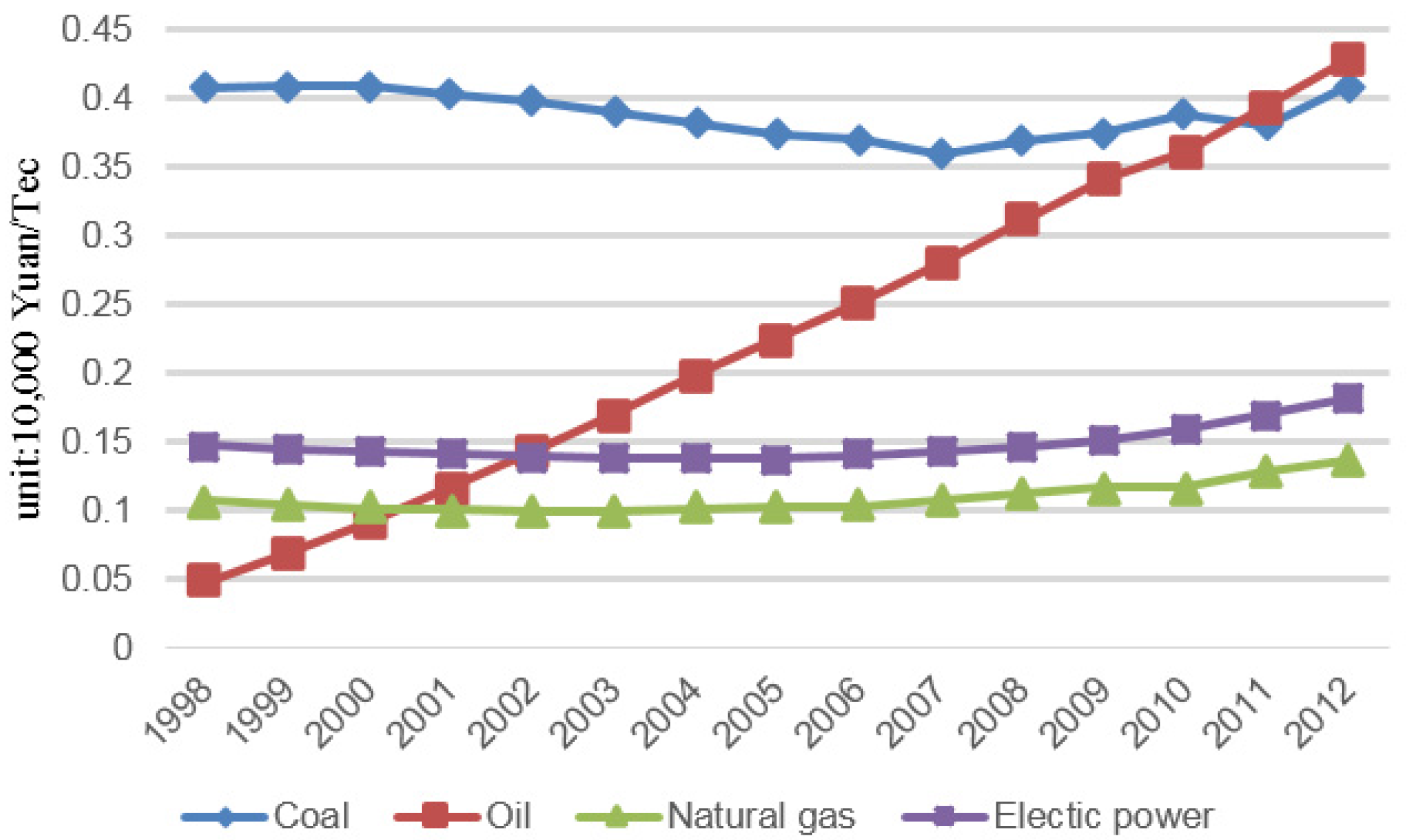
- By extending the work of prior research, we break down the shadow price into four sources of energy, and find that the shadow prices of different kinds of energy are quite different, and the same kind of energy also has different shadow prices in different regions. The situation indicates the existence of energy trade barriers among regions and the different contribution of the several types of energy to economy.
- Among the kinds of energy mentioned, the shadow price of oil has climbed dramatically, which means the efficiency of oil consumption has greatly improved. The increasingly rigid vehicle emissions standards and increasing tax allowance on smaller vehicles, may lead to the increase of marginal oil output.
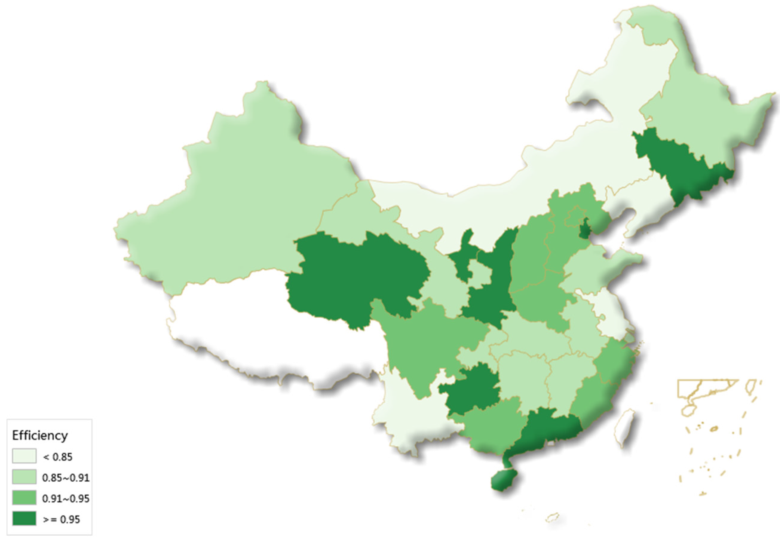
- In areas with rich energy resources, energy marginal output is low in most areas due to the lack of an integrated energy market, resulting in the reduction of total factor energy efficiency. Besides, misallocation of factor market owing to administrative interference remarkably brings about the inefficiency of energy.
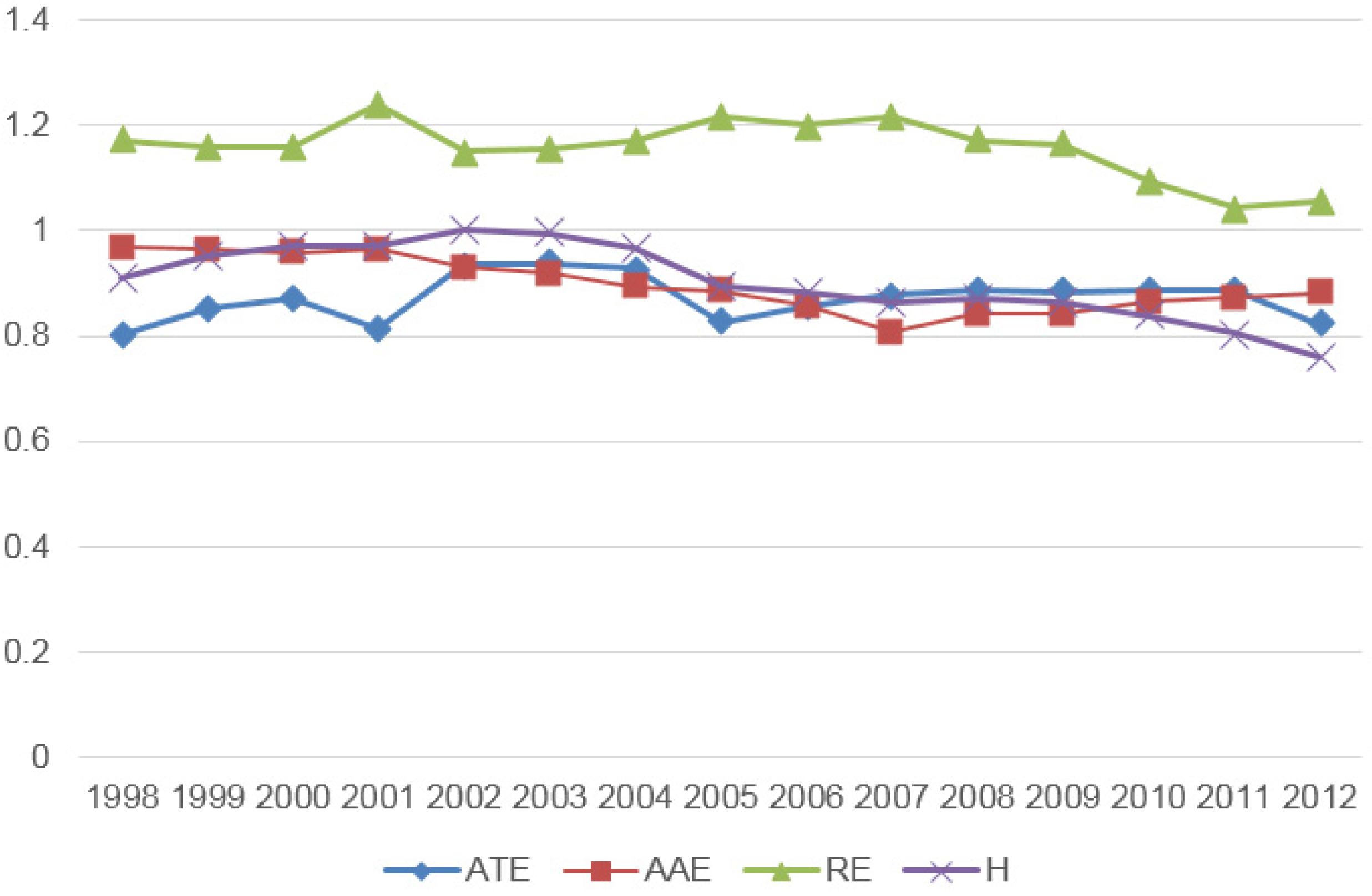
- Both the structure of energy input and inter-provincial allocation of energy impact on energy efficiency. Increasing values of the two indices in recent years imply the effect of China’s adjusted energy policy. Inter-provincial energy barrier will be broken for the marketization of energy factor and better negotiability of energy among areas. Specifically, it is of great necessity to realize marketing disposition of energy, energy structure adjustment and energy efficiency improvement for achieving reduction goal of carbon emission.
Acknowledgments
Author Contributions
Conflicts of Interest
Appendix
Appendix A1. Efficiency Decompositon Framework


Appendix A2. Depreciation Rate of Different Areas

| Province | Beijing | Tianjin | Hebei | Shanxi | Neimenggu | liaoning | Jilin | Heilongjiang | Shanghai | Jiangsu |
| Depreciation rate (%) | 3.4 | 3.7 | 4.3 | 4 | 4.3 | 5.8 | 5.1 | 6 | 3.4 | 4.2 |
| Province | Zhejiang | Anhui | Fujian | Jiangxi | Shandong | Henan | Hubei | Hunan | Guangdong | Guangxi |
| Depreciation rate (%) | 4 | 5 | 4.5 | 3.7 | 5 | 4.1 | 4.5 | 4.5 | 6.9 | 3.3 |
| Province | Hainan | Chongqing | Sichuan | Guizhou | Yunnan | Shaanxi | Gansu | Qinghai | Ningxia | Xinjiang |
| Depreciation rate (%) | 2.2 | 4.6 | 4.6 | 2.8 | 2.7 | 3.3 | 2.7 | 2.4 | 2.8 | 2.6 |
Appendix A3. The Shadow Price of Each Energy from 1998 to 2012 are as Follow
| 1998 | 1999 | 2000 | 2001 | 2002 | 2003 | 2004 | 2005 | 2006 | 2007 | 2008 | 2009 | 2010 | 2011 | 2012 | |
|---|---|---|---|---|---|---|---|---|---|---|---|---|---|---|---|
| Beijing | 0.437 | 0.442 | 0.451 | 0.442 | 0.463 | 0.461 | 0.486 | 0.511 | 0.541 | 0.569 | 0.628 | 0.678 | 0.721 | 0.763 | 0.876 |
| Tianjin | 0.405 | 0.406 | 0.412 | 0.408 | 0.396 | 0.395 | 0.384 | 0.378 | 0.381 | 0.384 | 0.386 | 0.382 | 0.403 | 0.400 | 0.421 |
| Hebei | 0.326 | 0.316 | 0.307 | 0.290 | 0.265 | 0.233 | 0.204 | 0.173 | 0.135 | 0.111 | 0.094 | 0.080 | 0.103 | 0.056 | 0.070 |
| Shanxi | 0.321 | 0.324 | 0.313 | 0.209 | 0.250 | 0.226 | 0.196 | 0.182 | 0.161 | 0.000 | 0.147 | 0.149 | 0.166 | 0.126 | 0.108 |
| Neimenggu | 0.358 | 0.351 | 0.344 | 0.336 | 0.322 | 0.305 | 0.271 | 0.239 | 0.220 | 0.208 | 0.158 | 0.153 | 0.136 | 0.034 | 0.000 |
| Liaoning | 0.380 | 0.418 | 0.407 | 0.398 | 0.361 | 0.338 | 0.296 | 0.330 | 0.311 | 0.276 | 0.269 | 0.247 | 0.317 | 0.351 | 0.432 |
| Jilin | 0.391 | 0.384 | 0.382 | 0.375 | 0.369 | 0.363 | 0.351 | 0.343 | 0.332 | 0.346 | 0.331 | 0.329 | 0.325 | 0.291 | 0.312 |
| Heilongjiang | 0.426 | 0.430 | 0.426 | 0.424 | 0.416 | 0.402 | 0.379 | 0.379 | 0.382 | 0.374 | 0.344 | 0.374 | 0.362 | 0.335 | 0.306 |
| Shanghai | 0.383 | 0.376 | 0.384 | 0.379 | 0.384 | 0.386 | 0.410 | 0.432 | 0.471 | 0.481 | 0.478 | 0.496 | 0.505 | 0.507 | 0.559 |
| Jiangsu | 0.361 | 0.351 | 0.352 | 0.346 | 0.337 | 0.330 | 0.298 | 0.246 | 0.231 | 0.241 | 0.265 | 0.271 | 0.276 | 0.219 | 0.277 |
| Zhejiang | 0.408 | 0.404 | 0.401 | 0.396 | 0.403 | 0.405 | 0.390 | 0.390 | 0.375 | 0.355 | 0.363 | 0.380 | 0.440 | 0.465 | 0.491 |
| Anhui | 0.386 | 0.380 | 0.373 | 0.363 | 0.356 | 0.343 | 0.335 | 0.324 | 0.314 | 0.297 | 0.283 | 0.264 | 0.249 | 0.238 | 0.239 |
| Fujian | 0.422 | 0.416 | 0.413 | 0.414 | 0.402 | 0.388 | 0.381 | 0.378 | 0.371 | 0.354 | 0.360 | 0.349 | 0.432 | 0.394 | 0.436 |
| Jiangxi | 0.413 | 0.412 | 0.409 | 0.411 | 0.407 | 0.392 | 0.381 | 0.385 | 0.373 | 0.355 | 0.359 | 0.349 | 0.361 | 0.334 | 0.352 |
| Shandong | 0.381 | 0.370 | 0.388 | 0.354 | 0.322 | 0.302 | 0.270 | 0.246 | 0.201 | 0.179 | 0.162 | 0.172 | 0.181 | 0.183 | 0.200 |
| Henan | 0.392 | 0.393 | 0.388 | 0.383 | 0.369 | 0.354 | 0.325 | 0.277 | 0.252 | 0.222 | 0.229 | 0.237 | 0.268 | 0.258 | 0.423 |
| Hubei | 0.411 | 0.409 | 0.411 | 0.403 | 0.399 | 0.393 | 0.388 | 0.415 | 0.415 | 0.400 | 0.480 | 0.472 | 0.373 | 0.338 | 0.398 |
| Hunan | 0.418 | 0.430 | 0.436 | 0.420 | 0.426 | 0.405 | 0.401 | 0.376 | 0.377 | 0.370 | 0.431 | 0.458 | 0.557 | 0.561 | 0.716 |
| Guangdong | 0.450 | 0.443 | 0.438 | 0.440 | 0.445 | 0.449 | 0.449 | 0.469 | 0.488 | 0.527 | 0.563 | 0.732 | 0.560 | 0.514 | 0.615 |
| Guangxi | 0.449 | 0.448 | 0.451 | 0.453 | 0.461 | 0.461 | 0.449 | 0.432 | 0.442 | 0.441 | 0.465 | 0.455 | 0.476 | 0.516 | 0.555 |
| Hainan | 0.428 | 0.413 | 0.424 | 0.425 | 0.435 | 0.446 | 0.456 | 0.448 | 0.460 | 0.451 | 0.465 | 0.459 | 0.473 | 0.526 | 0.523 |
| Chongqing | 0.459 | 0.465 | 0.480 | 0.446 | 0.447 | 0.458 | 0.465 | 0.509 | 0.526 | 0.536 | 0.548 | 0.545 | 0.578 | 0.557 | 0.615 |
| Sichuan | 0.533 | 0.565 | 0.572 | 0.594 | 0.603 | 0.594 | 0.612 | 0.658 | 0.711 | 0.745 | 0.741 | 0.798 | 1.099 | 1.802 | 1.707 |
| Guizhou | 0.391 | 0.392 | 0.394 | 0.408 | 0.400 | 0.371 | 0.347 | 0.321 | 0.299 | 0.287 | 0.296 | 0.274 | 0.265 | 0.245 | 0.221 |
| Yunnan | 0.428 | 0.431 | 0.437 | 0.434 | 0.431 | 0.423 | 0.436 | 0.421 | 0.392 | 0.393 | 0.399 | 0.378 | 0.397 | 0.432 | 0.484 |
| Shaanxi | 0.408 | 0.414 | 0.427 | 0.435 | 0.439 | 0.430 | 0.453 | 0.390 | 0.405 | 0.429 | 0.448 | 0.426 | 0.435 | 0.431 | 0.421 |
| Gansu | 0.426 | 0.425 | 0.425 | 0.417 | 0.414 | 0.416 | 0.416 | 0.421 | 0.424 | 0.420 | 0.415 | 0.434 | 0.395 | 0.377 | 0.391 |
| Qinghai | 0.419 | 0.421 | 0.423 | 0.420 | 0.432 | 0.441 | 0.453 | 0.464 | 0.465 | 0.461 | 0.466 | 0.474 | 0.502 | 0.551 | 0.590 |
| Ningxia | 0.402 | 0.402 | 0.400 | 0.397 | 0.395 | 0.392 | 0.393 | 0.374 | 0.373 | 0.382 | 0.358 | 0.356 | 0.345 | 0.314 | 0.324 |
| Xinjiang | 0.445 | 0.448 | 0.447 | 0.516 | 0.467 | 0.481 | 0.506 | 0.523 | 0.544 | 0.555 | 0.541 | 0.509 | 0.567 | 0.591 | 0.596 |
| eastern | 0.398 | 0.396 | 0.398 | 0.390 | 0.383 | 0.376 | 0.366 | 0.364 | 0.360 | 0.357 | 0.367 | 0.386 | 0.401 | 0.398 | 0.446 |
| central | 0.396 | 0.393 | 0.391 | 0.374 | 0.375 | 0.365 | 0.351 | 0.344 | 0.336 | 0.306 | 0.330 | 0.329 | 0.322 | 0.306 | 0.333 |
| western | 0.429 | 0.433 | 0.436 | 0.441 | 0.437 | 0.434 | 0.436 | 0.432 | 0.436 | 0.442 | 0.440 | 0.436 | 0.472 | 0.532 | 0.537 |
| Total | 0.408 | 0.408 | 0.409 | 0.402 | 0.398 | 0.389 | 0.381 | 0.374 | 0.369 | 0.359 | 0.369 | 0.375 | 0.389 | 0.380 | 0.408 |
| 1998 | 1999 | 2000 | 2001 | 2002 | 2003 | 2004 | 2005 | 2006 | 2007 | 2008 | 2009 | 2010 | 2011 | 2012 | |
|---|---|---|---|---|---|---|---|---|---|---|---|---|---|---|---|
| Beijing | 0.005 | 0.022 | 0.042 | 0.061 | 0.078 | 0.106 | 0.122 | 0.142 | 0.157 | 0.175 | 0.187 | 0.211 | 0.240 | 0.283 | 0.303 |
| Tianjin | 0.014 | 0.035 | 0.051 | 0.079 | 0.106 | 0.131 | 0.160 | 0.189 | 0.222 | 0.253 | 0.281 | 0.313 | 0.318 | 0.337 | 0.371 |
| Hebei | 0.091 | 0.113 | 0.137 | 0.164 | 0.194 | 0.226 | 0.261 | 0.309 | 0.345 | 0.376 | 0.405 | 0.448 | 0.475 | 0.505 | 0.532 |
| Shanxi | 0.075 | 0.096 | 0.123 | 0.188 | 0.195 | 0.229 | 0.263 | 0.292 | 0.325 | 0.403 | 0.377 | 0.406 | 0.431 | 0.476 | 0.515 |
| Neimenggu | 0.054 | 0.080 | 0.105 | 0.133 | 0.163 | 0.190 | 0.223 | 0.254 | 0.280 | 0.303 | 0.339 | 0.360 | 0.387 | 0.442 | 0.481 |
| Liaoning | 0.042 | 0.042 | 0.061 | 0.093 | 0.125 | 0.154 | 0.210 | 0.193 | 0.214 | 0.246 | 0.260 | 0.288 | 0.253 | 0.239 | 0.209 |
| Jilin | 0.035 | 0.061 | 0.087 | 0.114 | 0.141 | 0.169 | 0.202 | 0.224 | 0.251 | 0.282 | 0.323 | 0.353 | 0.376 | 0.416 | 0.473 |
| Heilongjiang | 0.015 | 0.033 | 0.051 | 0.076 | 0.101 | 0.129 | 0.161 | 0.183 | 0.216 | 0.231 | 0.281 | 0.304 | 0.326 | 0.345 | 0.364 |
| Shanghai | 0.000 | 0.019 | 0.034 | 0.051 | 0.066 | 0.082 | 0.090 | 0.102 | 0.101 | 0.113 | 0.135 | 0.149 | 0.160 | 0.172 | 0.184 |
| Jiangsu | 0.069 | 0.088 | 0.100 | 0.120 | 0.139 | 0.154 | 0.173 | 0.184 | 0.185 | 0.189 | 0.188 | 0.194 | 0.174 | 0.171 | 0.128 |
| Zhejiang | 0.039 | 0.057 | 0.076 | 0.097 | 0.122 | 0.141 | 0.164 | 0.184 | 0.201 | 0.222 | 0.247 | 0.263 | 0.239 | 0.243 | 0.273 |
| Anhui | 0.089 | 0.114 | 0.141 | 0.169 | 0.197 | 0.227 | 0.256 | 0.286 | 0.316 | 0.347 | 0.380 | 0.413 | 0.441 | 0.467 | 0.486 |
| Fujian | 0.030 | 0.053 | 0.077 | 0.103 | 0.127 | 0.153 | 0.177 | 0.213 | 0.245 | 0.271 | 0.313 | 0.334 | 0.323 | 0.336 | 0.383 |
| Jiangxi | 0.057 | 0.081 | 0.106 | 0.129 | 0.158 | 0.186 | 0.225 | 0.252 | 0.288 | 0.327 | 0.365 | 0.409 | 0.441 | 0.468 | 0.523 |
| Shandong | 0.084 | 0.105 | 0.115 | 0.143 | 0.173 | 0.186 | 0.202 | 0.211 | 0.223 | 0.238 | 0.259 | 0.251 | 0.221 | 0.218 | 0.190 |
| Henan | 0.108 | 0.133 | 0.164 | 0.188 | 0.217 | 0.245 | 0.277 | 0.305 | 0.332 | 0.360 | 0.394 | 0.437 | 0.469 | 0.489 | 0.526 |
| Hubei | 0.078 | 0.101 | 0.127 | 0.155 | 0.180 | 0.207 | 0.240 | 0.267 | 0.303 | 0.321 | 0.366 | 0.401 | 0.421 | 0.450 | 0.516 |
| Hunan | 0.089 | 0.106 | 0.128 | 0.161 | 0.184 | 0.219 | 0.258 | 0.296 | 0.331 | 0.364 | 0.452 | 0.509 | 0.624 | 0.693 | 0.845 |
| Guangdong | 0.000 | 0.013 | 0.035 | 0.049 | 0.062 | 0.077 | 0.085 | 0.082 | 0.081 | 0.060 | 0.067 | 0.000 | 0.068 | 0.068 | 0.071 |
| Guangxi | 0.066 | 0.092 | 0.120 | 0.147 | 0.175 | 0.211 | 0.247 | 0.273 | 0.318 | 0.360 | 0.417 | 0.459 | 0.508 | 0.596 | 0.650 |
| Hainan | 0.012 | 0.044 | 0.065 | 0.090 | 0.114 | 0.138 | 0.165 | 0.202 | 0.234 | 0.268 | 0.304 | 0.347 | 0.386 | 0.415 | 0.468 |
| Chongqing | 0.033 | 0.054 | 0.076 | 0.106 | 0.133 | 0.156 | 0.182 | 0.223 | 0.256 | 0.291 | 0.342 | 0.389 | 0.428 | 0.454 | 0.504 |
| Sichuan | 0.059 | 0.076 | 0.102 | 0.123 | 0.148 | 0.181 | 0.209 | 0.229 | 0.241 | 0.270 | 0.316 | 0.329 | 0.294 | 0.554 | 0.570 |
| Guizhou | 0.069 | 0.091 | 0.120 | 0.153 | 0.184 | 0.221 | 0.258 | 0.281 | 0.319 | 0.351 | 0.381 | 0.423 | 0.459 | 0.503 | 0.551 |
| Yunnan | 0.060 | 0.084 | 0.111 | 0.137 | 0.168 | 0.203 | 0.237 | 0.291 | 0.322 | 0.364 | 0.413 | 0.460 | 0.500 | 0.578 | 0.681 |
| Shaanxi | 0.049 | 0.070 | 0.087 | 0.109 | 0.134 | 0.159 | 0.174 | 0.231 | 0.250 | 0.271 | 0.284 | 0.322 | 0.344 | 0.373 | 0.410 |
| Gansu | 0.046 | 0.072 | 0.095 | 0.126 | 0.158 | 0.180 | 0.220 | 0.250 | 0.287 | 0.326 | 0.370 | 0.420 | 0.450 | 0.491 | 0.546 |
| Qinghai | 0.022 | 0.047 | 0.073 | 0.099 | 0.123 | 0.150 | 0.183 | 0.215 | 0.254 | 0.298 | 0.337 | 0.386 | 0.452 | 0.513 | 0.579 |
| Ningxia | 0.025 | 0.050 | 0.076 | 0.103 | 0.131 | 0.160 | 0.191 | 0.232 | 0.270 | 0.315 | 0.344 | 0.389 | 0.431 | 0.487 | 0.533 |
| Xinjiang | 0.000 | 0.024 | 0.047 | 0.026 | 0.091 | 0.112 | 0.128 | 0.147 | 0.172 | 0.202 | 0.247 | 0.304 | 0.318 | 0.344 | 0.393 |
| eastern | 0.035 | 0.054 | 0.072 | 0.095 | 0.119 | 0.141 | 0.164 | 0.183 | 0.201 | 0.219 | 0.241 | 0.254 | 0.260 | 0.272 | 0.283 |
| middle | 0.059 | 0.083 | 0.108 | 0.139 | 0.163 | 0.191 | 0.223 | 0.251 | 0.283 | 0.317 | 0.349 | 0.384 | 0.411 | 0.441 | 0.484 |
| western | 0.044 | 0.067 | 0.092 | 0.115 | 0.146 | 0.175 | 0.205 | 0.239 | 0.270 | 0.305 | 0.345 | 0.385 | 0.416 | 0.485 | 0.536 |
| Total | 0.048 | 0.069 | 0.091 | 0.117 | 0.143 | 0.170 | 0.198 | 0.225 | 0.251 | 0.280 | 0.311 | 0.341 | 0.361 | 0.393 | 0.428 |
| 1998 | 1999 | 2000 | 2001 | 2002 | 2003 | 2004 | 2005 | 2006 | 2007 | 2008 | 2009 | 2010 | 2011 | 2012 | |
|---|---|---|---|---|---|---|---|---|---|---|---|---|---|---|---|
| Beijing | 0.112 | 0.107 | 0.106 | 0.100 | 0.094 | 0.096 | 0.088 | 0.084 | 0.077 | 0.073 | 0.059 | 0.053 | 0.051 | 0.053 | 0.036 |
| Tianjin | 0.100 | 0.096 | 0.089 | 0.089 | 0.088 | 0.084 | 0.084 | 0.084 | 0.085 | 0.085 | 0.084 | 0.088 | 0.078 | 0.079 | 0.087 |
| Hebei | 0.124 | 0.126 | 0.126 | 0.129 | 0.134 | 0.141 | 0.153 | 0.174 | 0.188 | 0.200 | 0.212 | 0.235 | 0.250 | 0.272 | 0.291 |
| Shanxi | 0.122 | 0.119 | 0.119 | 0.141 | 0.128 | 0.131 | 0.135 | 0.136 | 0.139 | 0.178 | 0.136 | 0.135 | 0.132 | 0.145 | 0.152 |
| Neimenggu | 0.113 | 0.111 | 0.109 | 0.108 | 0.108 | 0.109 | 0.112 | 0.117 | 0.119 | 0.121 | 0.132 | 0.135 | 0.144 | 0.176 | 0.195 |
| Liaoning | 0.117 | 0.099 | 0.092 | 0.098 | 0.104 | 0.107 | 0.132 | 0.104 | 0.108 | 0.121 | 0.128 | 0.142 | 0.118 | 0.110 | 0.091 |
| Jilin | 0.103 | 0.102 | 0.101 | 0.099 | 0.097 | 0.095 | 0.096 | 0.090 | 0.089 | 0.092 | 0.103 | 0.106 | 0.108 | 0.120 | 0.136 |
| Heilongjiang | 0.089 | 0.085 | 0.079 | 0.079 | 0.077 | 0.076 | 0.078 | 0.072 | 0.075 | 0.067 | 0.082 | 0.078 | 0.077 | 0.077 | 0.078 |
| Shanghai | 0.109 | 0.109 | 0.105 | 0.103 | 0.098 | 0.095 | 0.087 | 0.085 | 0.072 | 0.073 | 0.076 | 0.075 | 0.073 | 0.069 | 0.064 |
| Jiangsu | 0.117 | 0.120 | 0.116 | 0.121 | 0.125 | 0.131 | 0.140 | 0.146 | 0.152 | 0.168 | 0.185 | 0.214 | 0.232 | 0.262 | 0.287 |
| Zhejiang | 0.115 | 0.113 | 0.109 | 0.110 | 0.116 | 0.121 | 0.129 | 0.136 | 0.143 | 0.153 | 0.168 | 0.177 | 0.167 | 0.176 | 0.207 |
| Anhui | 0.110 | 0.108 | 0.107 | 0.107 | 0.106 | 0.106 | 0.106 | 0.106 | 0.107 | 0.109 | 0.112 | 0.116 | 0.120 | 0.124 | 0.122 |
| Fujian | 0.109 | 0.108 | 0.106 | 0.106 | 0.103 | 0.102 | 0.100 | 0.107 | 0.112 | 0.116 | 0.130 | 0.132 | 0.112 | 0.112 | 0.132 |
| Jiangxi | 0.105 | 0.102 | 0.100 | 0.096 | 0.094 | 0.091 | 0.097 | 0.094 | 0.096 | 0.100 | 0.102 | 0.108 | 0.106 | 0.106 | 0.113 |
| Shandong | 0.110 | 0.112 | 0.107 | 0.114 | 0.125 | 0.126 | 0.132 | 0.137 | 0.146 | 0.162 | 0.186 | 0.196 | 0.193 | 0.220 | 0.230 |
| Henan | 0.113 | 0.111 | 0.110 | 0.111 | 0.114 | 0.117 | 0.124 | 0.131 | 0.141 | 0.155 | 0.172 | 0.198 | 0.223 | 0.245 | 0.280 |
| Hubei | 0.112 | 0.110 | 0.111 | 0.111 | 0.109 | 0.108 | 0.111 | 0.110 | 0.117 | 0.113 | 0.121 | 0.129 | 0.140 | 0.154 | 0.181 |
| Hunan | 0.115 | 0.109 | 0.106 | 0.109 | 0.104 | 0.108 | 0.114 | 0.120 | 0.124 | 0.128 | 0.160 | 0.177 | 0.222 | 0.249 | 0.308 |
| Guangdong | 0.087 | 0.085 | 0.089 | 0.088 | 0.090 | 0.094 | 0.093 | 0.087 | 0.093 | 0.092 | 0.111 | 0.089 | 0.154 | 0.182 | 0.259 |
| Guangxi | 0.110 | 0.108 | 0.106 | 0.103 | 0.100 | 0.102 | 0.102 | 0.096 | 0.101 | 0.106 | 0.116 | 0.123 | 0.134 | 0.162 | 0.179 |
| Hainan | 0.093 | 0.095 | 0.090 | 0.085 | 0.078 | 0.071 | 0.063 | 0.061 | 0.054 | 0.049 | 0.041 | 0.037 | 0.027 | 0.005 | 0.000 |
| Chongqing | 0.098 | 0.094 | 0.091 | 0.088 | 0.087 | 0.082 | 0.078 | 0.083 | 0.080 | 0.077 | 0.083 | 0.087 | 0.083 | 0.079 | 0.075 |
| Sichuan | 0.086 | 0.081 | 0.079 | 0.074 | 0.071 | 0.073 | 0.072 | 0.064 | 0.051 | 0.052 | 0.062 | 0.054 | 0.000 | 0.080 | 0.094 |
| Guizhou | 0.111 | 0.107 | 0.106 | 0.105 | 0.103 | 0.104 | 0.105 | 0.102 | 0.104 | 0.102 | 0.096 | 0.099 | 0.098 | 0.101 | 0.107 |
| Yunnan | 0.110 | 0.108 | 0.106 | 0.102 | 0.102 | 0.103 | 0.102 | 0.113 | 0.111 | 0.113 | 0.117 | 0.122 | 0.121 | 0.137 | 0.162 |
| Shaanxi | 0.106 | 0.101 | 0.095 | 0.090 | 0.086 | 0.081 | 0.070 | 0.087 | 0.079 | 0.071 | 0.060 | 0.067 | 0.064 | 0.068 | 0.076 |
| Gansu | 0.099 | 0.099 | 0.094 | 0.094 | 0.093 | 0.084 | 0.087 | 0.084 | 0.083 | 0.080 | 0.080 | 0.078 | 0.074 | 0.072 | 0.070 |
| Qinghai | 0.100 | 0.097 | 0.094 | 0.089 | 0.083 | 0.077 | 0.073 | 0.066 | 0.063 | 0.061 | 0.054 | 0.049 | 0.048 | 0.036 | 0.025 |
| Ningxia | 0.101 | 0.098 | 0.094 | 0.091 | 0.087 | 0.083 | 0.079 | 0.081 | 0.078 | 0.078 | 0.071 | 0.068 | 0.064 | 0.068 | 0.060 |
| Xinjiang | 0.089 | 0.087 | 0.084 | 0.047 | 0.072 | 0.065 | 0.053 | 0.041 | 0.032 | 0.026 | 0.029 | 0.038 | 0.015 | 0.001 | 0.000 |
| eastern | 0.109 | 0.106 | 0.103 | 0.104 | 0.105 | 0.106 | 0.109 | 0.110 | 0.112 | 0.117 | 0.125 | 0.131 | 0.132 | 0.140 | 0.153 |
| middle | 0.106 | 0.104 | 0.102 | 0.104 | 0.100 | 0.099 | 0.101 | 0.100 | 0.102 | 0.108 | 0.108 | 0.113 | 0.117 | 0.122 | 0.133 |
| western | 0.102 | 0.099 | 0.096 | 0.090 | 0.090 | 0.088 | 0.085 | 0.085 | 0.082 | 0.081 | 0.082 | 0.084 | 0.077 | 0.089 | 0.095 |
| Total | 0.106 | 0.104 | 0.101 | 0.100 | 0.100 | 0.099 | 0.101 | 0.101 | 0.103 | 0.107 | 0.112 | 0.116 | 0.117 | 0.127 | 0.136 |
| 1998 | 1999 | 2000 | 2001 | 2002 | 2003 | 2004 | 2005 | 2006 | 2007 | 2008 | 2009 | 2010 | 2011 | 2012 | |
|---|---|---|---|---|---|---|---|---|---|---|---|---|---|---|---|
| Beijing | 0.195 | 0.197 | 0.198 | 0.201 | 0.200 | 0.201 | 0.199 | 0.203 | 0.209 | 0.216 | 0.226 | 0.238 | 0.250 | 0.258 | 0.285 |
| Tianjin | 0.194 | 0.192 | 0.193 | 0.192 | 0.190 | 0.190 | 0.190 | 0.190 | 0.191 | 0.192 | 0.195 | 0.201 | 0.208 | 0.218 | 0.234 |
| Hebei | 0.124 | 0.125 | 0.123 | 0.122 | 0.122 | 0.123 | 0.124 | 0.121 | 0.123 | 0.131 | 0.137 | 0.143 | 0.150 | 0.165 | 0.181 |
| Shanxi | 0.167 | 0.165 | 0.163 | 0.164 | 0.161 | 0.159 | 0.159 | 0.159 | 0.158 | 0.164 | 0.157 | 0.159 | 0.167 | 0.172 | 0.178 |
| Neimenggu | 0.175 | 0.173 | 0.171 | 0.169 | 0.167 | 0.170 | 0.171 | 0.173 | 0.178 | 0.186 | 0.192 | 0.204 | 0.212 | 0.219 | 0.231 |
| Liaoning | 0.165 | 0.158 | 0.156 | 0.155 | 0.160 | 0.162 | 0.163 | 0.159 | 0.164 | 0.171 | 0.181 | 0.189 | 0.196 | 0.216 | 0.238 |
| Jilin | 0.174 | 0.172 | 0.169 | 0.167 | 0.165 | 0.162 | 0.161 | 0.160 | 0.161 | 0.160 | 0.168 | 0.174 | 0.184 | 0.190 | 0.199 |
| Heilongjiang | 0.167 | 0.165 | 0.166 | 0.165 | 0.163 | 0.163 | 0.161 | 0.160 | 0.158 | 0.161 | 0.164 | 0.163 | 0.166 | 0.173 | 0.181 |
| Shanghai | 0.199 | 0.201 | 0.201 | 0.204 | 0.205 | 0.206 | 0.206 | 0.214 | 0.219 | 0.228 | 0.236 | 0.246 | 0.263 | 0.280 | 0.299 |
| Jiangsu | 0.107 | 0.108 | 0.109 | 0.110 | 0.112 | 0.116 | 0.125 | 0.143 | 0.162 | 0.180 | 0.204 | 0.228 | 0.261 | 0.308 | 0.363 |
| Zhejiang | 0.144 | 0.144 | 0.141 | 0.140 | 0.138 | 0.139 | 0.143 | 0.145 | 0.157 | 0.165 | 0.171 | 0.178 | 0.196 | 0.218 | 0.242 |
| Anhui | 0.107 | 0.103 | 0.099 | 0.096 | 0.093 | 0.089 | 0.086 | 0.083 | 0.080 | 0.080 | 0.079 | 0.080 | 0.084 | 0.090 | 0.094 |
| Fujian | 0.164 | 0.163 | 0.161 | 0.159 | 0.158 | 0.158 | 0.157 | 0.154 | 0.154 | 0.157 | 0.159 | 0.168 | 0.181 | 0.191 | 0.199 |
| Jiangxi | 0.141 | 0.138 | 0.137 | 0.135 | 0.129 | 0.127 | 0.123 | 0.118 | 0.116 | 0.114 | 0.112 | 0.111 | 0.109 | 0.115 | 0.115 |
| Shandong | 0.079 | 0.077 | 0.073 | 0.076 | 0.079 | 0.084 | 0.092 | 0.097 | 0.111 | 0.120 | 0.132 | 0.148 | 0.168 | 0.190 | 0.220 |
| Henan | 0.070 | 0.061 | 0.048 | 0.047 | 0.046 | 0.045 | 0.046 | 0.053 | 0.059 | 0.065 | 0.066 | 0.065 | 0.068 | 0.083 | 0.089 |
| Hubei | 0.107 | 0.104 | 0.100 | 0.097 | 0.094 | 0.091 | 0.087 | 0.082 | 0.078 | 0.083 | 0.073 | 0.078 | 0.101 | 0.116 | 0.118 |
| Hunan | 0.097 | 0.094 | 0.091 | 0.088 | 0.082 | 0.080 | 0.073 | 0.071 | 0.068 | 0.067 | 0.049 | 0.044 | 0.022 | 0.029 | 0.012 |
| Guangdong | 0.124 | 0.126 | 0.122 | 0.121 | 0.122 | 0.119 | 0.119 | 0.116 | 0.127 | 0.151 | 0.163 | 0.201 | 0.204 | 0.243 | 0.289 |
| Guangxi | 0.123 | 0.119 | 0.113 | 0.109 | 0.103 | 0.098 | 0.094 | 0.093 | 0.085 | 0.082 | 0.073 | 0.073 | 0.071 | 0.065 | 0.078 |
| Hainan | 0.195 | 0.191 | 0.189 | 0.187 | 0.186 | 0.185 | 0.184 | 0.180 | 0.178 | 0.175 | 0.173 | 0.169 | 0.167 | 0.173 | 0.169 |
| Chongqing | 0.158 | 0.157 | 0.156 | 0.156 | 0.157 | 0.157 | 0.157 | 0.153 | 0.154 | 0.155 | 0.156 | 0.158 | 0.164 | 0.174 | 0.183 |
| Sichuan | 0.076 | 0.069 | 0.064 | 0.060 | 0.059 | 0.058 | 0.056 | 0.054 | 0.058 | 0.059 | 0.058 | 0.071 | 0.093 | 0.015 | 0.054 |
| Guizhou | 0.147 | 0.145 | 0.139 | 0.127 | 0.122 | 0.119 | 0.116 | 0.125 | 0.123 | 0.124 | 0.121 | 0.120 | 0.122 | 0.121 | 0.121 |
| Yunnan | 0.137 | 0.134 | 0.128 | 0.124 | 0.120 | 0.116 | 0.110 | 0.101 | 0.101 | 0.095 | 0.087 | 0.084 | 0.078 | 0.066 | 0.053 |
| Shaanxi | 0.152 | 0.150 | 0.147 | 0.146 | 0.142 | 0.141 | 0.143 | 0.139 | 0.141 | 0.144 | 0.150 | 0.153 | 0.161 | 0.170 | 0.183 |
| Gansu | 0.153 | 0.150 | 0.148 | 0.145 | 0.142 | 0.141 | 0.136 | 0.138 | 0.135 | 0.132 | 0.127 | 0.119 | 0.123 | 0.123 | 0.122 |
| Qinghai | 0.194 | 0.191 | 0.188 | 0.187 | 0.186 | 0.184 | 0.182 | 0.180 | 0.177 | 0.172 | 0.169 | 0.166 | 0.159 | 0.157 | 0.156 |
| Ningxia | 0.194 | 0.191 | 0.189 | 0.188 | 0.186 | 0.183 | 0.181 | 0.177 | 0.174 | 0.170 | 0.170 | 0.167 | 0.166 | 0.166 | 0.164 |
| Xinjiang | 0.191 | 0.190 | 0.189 | 0.184 | 0.189 | 0.188 | 0.191 | 0.187 | 0.189 | 0.190 | 0.190 | 0.190 | 0.192 | 0.198 | 0.204 |
| eastern | 0.154 | 0.153 | 0.151 | 0.152 | 0.152 | 0.153 | 0.155 | 0.157 | 0.163 | 0.171 | 0.180 | 0.192 | 0.204 | 0.224 | 0.247 |
| middle | 0.141 | 0.137 | 0.134 | 0.132 | 0.130 | 0.128 | 0.126 | 0.124 | 0.123 | 0.125 | 0.124 | 0.125 | 0.131 | 0.139 | 0.143 |
| western | 0.155 | 0.152 | 0.149 | 0.145 | 0.143 | 0.141 | 0.140 | 0.138 | 0.138 | 0.137 | 0.136 | 0.137 | 0.140 | 0.134 | 0.141 |
| Total | 0.147 | 0.145 | 0.142 | 0.140 | 0.139 | 0.138 | 0.137 | 0.137 | 0.139 | 0.143 | 0.146 | 0.151 | 0.159 | 0.169 | 0.181 |
References
- Hu, J.L.; Kao, C.H. Efficient energy-saving targets for APEC economies. Energy Policy 2007, 35, 373–382. [Google Scholar] [CrossRef]
- Zhang, X.P.; Cheng, X.M.; Yuan, J.H.; Gao, X.S. Total-factor energy efficiency in developing countries. Energy Policy 2011, 39, 644–650. [Google Scholar] [CrossRef]
- Sheng, P.F. The explanation for the low energy efficiency of China: Allocation inefficiency or technology inefficiency. Ind. Econ. Res. 2015, 1, 9–20. [Google Scholar]
- Wang, F.; Feng, G.F. Contribution of improving energy mix to carbon intensity target in China: Potential assessment. China Ind. Econ. 2011, 4, 127–137. [Google Scholar]
- Shi, D. Regional Differences in China’s Energy Efficiency and Conservation Potentials. China Ind. Econ. 2006, 10, 49–58. [Google Scholar]
- Fan, Y.; Liao, H.; Wei, Y.M. Can market oriented economic reforms contribute to energy efficiency improvement? Evidence from China. Energy Policy 2007, 35, 2287–2295. [Google Scholar] [CrossRef]
- Hang, L.; Tu, M. The impacts of energy prices on energy intensity: Evidence from China. Energy Policy 2007, 35, 2978–2988. [Google Scholar] [CrossRef]
- Zhang, Z.X. Why did the energy intensity fall in China’s industrial sector in the 1990s? The relative importance of structural change and intensity change. Energy Econ. 2003, 25, 625–638. [Google Scholar] [CrossRef]
- Hu, J.L.; Wang, S.C. Total-factor energy efficiency of regions in China. Energy Policy 2006, 34, 3206–3217. [Google Scholar] [CrossRef]
- Lin, B.Q.; Du, K. Technology gap and China’s regional energy efficiency: A parametric metafrontier approach. Energy Econ. 2013, 40, 529–536. [Google Scholar] [CrossRef]
- Fujii, H.; Kaneko, S.; Managi, S. Changes in environmentally sensitive productivity and technological modernization in China’s iron and steel industry in the 1990s. Environ. Dev. Econ. 2010, 15, 485–504. [Google Scholar] [CrossRef]
- Li, L.B.; Hu, J.L. Ecological total-factor energy efficiency of regions in China. Energy Policy 2012, 46, 216–224. [Google Scholar] [CrossRef]
- Li, K.; Lin, B. Metafroniter energy efficiency with CO2 emissions and its convergence analysis for China. Energy Econ. 2015, 48, 230–241. [Google Scholar] [CrossRef]
- Ouyang, X.L.; Sun, C. Energy savings potential in China’s industrial sector: From the perspectives of factor price distortion and allocative inefficiency. Energy Econ. 2015, 48, 117–126. [Google Scholar] [CrossRef]
- Sheng, P.F.; Yang, J. The Heterogeneity and convergence of energy’s shadow price in China—The estimation of nonparametric input distance function. Ind. Econ. Res. 2014, 1, 70–80. [Google Scholar]
- Sheng, P.F.; Yang, J.; Shackman, J.D. Energy’s Shadow Price and Energy Efficiency in China: A Non-Parametric Input Distance Function Analysis. Energies 2015, 8, 1975–1989. [Google Scholar] [CrossRef]
- Kumar, S.; Fujii, H.; Managi, S. Substitute or complement? Assessing renewable and nonrenewable energy in OECD countries. Appl. Econ. 2015, 47, 1438–1459. [Google Scholar] [CrossRef]
- Kaneko, S.; Fujii, H.; Sawazu, N.; Fujikura, R. Financial allocation strategy for the regional pollution abatement cost of reducing sulfur dioxide emissions in the thermal power sector in China. Energy Policy 2010, 38, 2131–2141. [Google Scholar] [CrossRef]
- Ishinabe, N.; Fujii, H.; Managi, S. The true cost of greenhouse gas emissions: Analysis of 1000 global companies. PLoS ONE 2013, 8, e78703. [Google Scholar] [CrossRef] [PubMed]
- Yagi, M.; Fujii, H.; Hoang, V.; Hoeng, V.; Managi, S. Environmental efficiency of energy, materials, and emissions. J. Environ. Manag. 2015, 161, 206–218. [Google Scholar] [CrossRef] [PubMed]
- Molinos-Senante, M.; Hanley, N.; Sala-Garrido, R. Measuring the CO2 shadow price for wastewater treatment: A directional distance function approach. Appl. Energy 2015, 144, 241–249. [Google Scholar] [CrossRef]
- Zhou, P.; Ang, B.W.; Zhou, D.Q. Measuring economy-wide energy efficiency performance: A parametric frontier approach. Appl. Energy 2012, 90, 196–200. [Google Scholar] [CrossRef]
- Lin, B.Q.; Du, K.R. The energy effect of factor market distortion in China. Econ. Res. J. 2013, 9, 125–136. [Google Scholar]
- Yuan, P.; Cheng, S. Estimating shadow pricing of industrial pollutions in China. Stat. Res. 2011, 28, 66–73. [Google Scholar]
- Wang, B.; Huang, R.J. Regional green development efficiency and green total productivity growth in China: From 2000 to 2010—Base on parametric metafrontier analysis. Ind. Econ. Rev. 2014, 5, 16–35. [Google Scholar]
- Li, S.; Ng, Y.C. Measuring the productive efficiency of a group of firms. Int. Adv. Econ. Res. 1995, 1, 377–390. [Google Scholar] [CrossRef]
- National Bureau of Statistics. China Statistical Yearbook; China Statistics Press: Beijing, China, 1998–2012.
- Department of Energy Statistics, National Bureau of Statistics. China Energy Statistical Yearbook; China Statistics Press: Beijing, China, 1998–2012.
- Wang, B.; Liu, G.T. Energy conservation and emission reduction and China’s green economic growth—Based on a total factor productivity perspective. China Ind. Econ. 2015, 5, 57–69. [Google Scholar]
- Zhang, J.; Wu, G.Y.; Zhang, J.P. The Estimation of China’s provincial capital stock: 1952–2000. Econ. Res. J. 2004, 10, 35–44. [Google Scholar]
- Zheng, K.; Yao, G. The Main Reason for Surge of Domestic Oil price—A VARA Approach. South China J. Econ. 2006, 5, 83–94. [Google Scholar]
- Wang, J.; Zhong, W.Z. The Research of Regional Energy Intensity Difference in China—From the Factor Endowment Perspectcive. Ind. Econ. Res. 2009, 6, 44–51. [Google Scholar]
- Shi, B.; Shen, K.R. The Government Intervention, the Economic Agglomeration and the Energy Efficiency. Manag. World 2008, 10, 6–18. [Google Scholar]
- Wang, W.G.; Fan, D. Influential factor and convergence of total factor energy efficiency in China based on the malmquist-luenber index. Resour. Sci. 2012, 34, 1816–1824. [Google Scholar]
- Tang, L.; Yang, Z.L. Energy efficiency and industrial economic transition. J. Quant. Tech. Econ. 2009, 10, 34–48. [Google Scholar]
- Wang, K.L.; Yang, L.; Yang, B.C.; Cheng, Y.H. Energy economic efficiency, the energy environmental performance and regional economic growth. J. Manag. 2013, 26, 86–99. [Google Scholar]
- Wu, Y.R. The role of productivity in China’s growth: New estimates. China Econ. Q. 2008, 2, 827–842. [Google Scholar] [CrossRef]


| Count | Mean | SD | Min | Max | |
|---|---|---|---|---|---|
| Coal (Tce) | 450 | 6365.87 | 5337.52 | 121.81 | 27,992.19 |
| Oil (Tce) | 450 | 1559.95 | 1559.51 | 82.33 | 8532.70 |
| Natural gas (Tce) | 450 | 277.54 | 348.70 | 0.00 | 2330.96 |
| Electic power (Tce) | 450 | 341.49 | 437.86 | 0.00 | 2963.72 |
| Labor (10,000 persons) | 450 | 2395.31 | 1610.40 | 254.80 | 6554.30 |
| Capital (100 million yuan) | 450 | 18,670.77 | 18,031.69 | 953.21 | 110,485.88 |
| GNP (100 million yuan) | 450 | 6645.87 | 6667.03 | 223.88 | 42,876.30 |
| Parameter | Estimated Value | Parameter | Estimated Value | Parameter | Estimated Value |
|---|---|---|---|---|---|
| α | −0.1485 | γ11 | −0.1281 | η13 | −0.0087 |
| α1 | −1.4090 | γ12 | 0.0686 | η14 | −0.1128 |
| α11 | −0.1246 | γ13 | 0.0443 | η21 | 0.0192 |
| β1 | 0.1523 | γ14 | 0.0151 | η22 | −0.0456 |
| β2 | 0.3132 | γ22 | −0.0386 | η23 | 0.0241 |
| β11 | 0.3786 | γ23 | −0.0292 | η24 | 0.0023 |
| β12 | −0.1259 | γ24 | −0.0008 | δ11 | −0.0022 |
| β22 | −0.0388 | γ33 | −0.0186 | δ21 | 0.1035 |
| γ1 | 0.5776 | γ34 | 0.0035 | μ11 | −0.0658 |
| γ2 | −0.0063 | γ44 | −0.0178 | μ21 | −0.0347 |
| γ3 | 0.1422 | η11 | 0.0531 | μ31 | 0.0266 |
| γ4 | 0.2864 | η12 | 0.0685 | μ41 | 0.0739 |
| Coal | Oil | Natural Gas | Electric Power | |||||||||
|---|---|---|---|---|---|---|---|---|---|---|---|---|
| 1998–2002 | 2003–2007 | 2008–2012 | 1998–2002 | 2003–2007 | 2008–2012 | 1998–2002 | 2003–2007 | 2008–2012 | 1998–2002 | 2003–2007 | 2008–2012 | |
| Beijing | 0.447 | 0.514 | 0.733 | 0.041 | 0.140 | 0.245 | 0.104 | 0.084 | 0.050 | 0.198 | 0.206 | 0.251 |
| Tianjin | 0.405 | 0.384 | 0.398 | 0.057 | 0.191 | 0.324 | 0.092 | 0.085 | 0.083 | 0.192 | 0.191 | 0.211 |
| Hebei | 0.301 | 0.171 | 0.081 | 0.140 | 0.303 | 0.473 | 0.128 | 0.171 | 0.252 | 0.123 | 0.125 | 0.155 |
| Shanxi | 0.200 | 0.153 | 0.139 | 0.060 | 0.302 | 0.441 | 0.069 | 0.144 | 0.140 | 0.098 | 0.160 | 0.167 |
| Neimenggu | 0.342 | 0.249 | 0.096 | 0.107 | 0.250 | 0.402 | 0.110 | 0.116 | 0.157 | 0.171 | 0.176 | 0.212 |
| Liaoning | 0.393 | 0.310 | 0.323 | 0.073 | 0.203 | 0.250 | 0.102 | 0.115 | 0.118 | 0.159 | 0.164 | 0.204 |
| Jilin | 0.380 | 0.347 | 0.318 | 0.088 | 0.225 | 0.388 | 0.100 | 0.092 | 0.115 | 0.169 | 0.161 | 0.183 |
| Heilongjiang | 0.424 | 0.383 | 0.344 | 0.055 | 0.184 | 0.324 | 0.082 | 0.074 | 0.078 | 0.165 | 0.160 | 0.170 |
| Shanghai | 0.381 | 0.436 | 0.509 | 0.034 | 0.098 | 0.160 | 0.105 | 0.082 | 0.071 | 0.202 | 0.215 | 0.265 |
| Jiangsu | 0.350 | 0.269 | 0.261 | 0.103 | 0.177 | 0.171 | 0.120 | 0.147 | 0.236 | 0.109 | 0.145 | 0.273 |
| Zhejiang | 0.402 | 0.383 | 0.428 | 0.078 | 0.182 | 0.253 | 0.112 | 0.136 | 0.179 | 0.141 | 0.150 | 0.201 |
| Anhui | 0.372 | 0.323 | 0.255 | 0.142 | 0.286 | 0.437 | 0.108 | 0.107 | 0.119 | 0.100 | 0.083 | 0.085 |
| Fujian | 0.413 | 0.375 | 0.394 | 0.078 | 0.212 | 0.338 | 0.106 | 0.107 | 0.124 | 0.161 | 0.156 | 0.180 |
| Jiangxi | 0.411 | 0.378 | 0.351 | 0.106 | 0.256 | 0.441 | 0.099 | 0.096 | 0.107 | 0.136 | 0.120 | 0.113 |
| Shandong | 0.363 | 0.239 | 0.180 | 0.124 | 0.212 | 0.228 | 0.114 | 0.141 | 0.205 | 0.077 | 0.101 | 0.172 |
| Henan | 0.385 | 0.286 | 0.283 | 0.162 | 0.304 | 0.463 | 0.112 | 0.134 | 0.224 | 0.054 | 0.054 | 0.074 |
| Hubei | 0.407 | 0.402 | 0.412 | 0.128 | 0.268 | 0.431 | 0.111 | 0.112 | 0.145 | 0.101 | 0.084 | 0.097 |
| Hunan | 0.426 | 0.386 | 0.545 | 0.134 | 0.294 | 0.625 | 0.109 | 0.119 | 0.223 | 0.090 | 0.072 | 0.031 |
| Guangdong | 0.443 | 0.476 | 0.597 | 0.032 | 0.077 | 0.055 | 0.088 | 0.092 | 0.159 | 0.123 | 0.126 | 0.220 |
| Guangxi | 0.452 | 0.445 | 0.493 | 0.120 | 0.282 | 0.526 | 0.105 | 0.102 | 0.143 | 0.113 | 0.090 | 0.072 |
| Hainan | 0.425 | 0.452 | 0.489 | 0.065 | 0.201 | 0.384 | 0.088 | 0.060 | 0.022 | 0.190 | 0.181 | 0.170 |
| Chongqing | 0.459 | 0.499 | 0.569 | 0.080 | 0.222 | 0.423 | 0.091 | 0.080 | 0.081 | 0.157 | 0.155 | 0.167 |
| Sichuan | 0.573 | 0.664 | 1.229 | 0.102 | 0.226 | 0.413 | 0.078 | 0.062 | 0.058 | 0.066 | 0.057 | 0.058 |
| Guizhou | 0.397 | 0.325 | 0.260 | 0.123 | 0.286 | 0.463 | 0.106 | 0.103 | 0.100 | 0.136 | 0.121 | 0.121 |
| Yunnan | 0.432 | 0.413 | 0.418 | 0.112 | 0.283 | 0.526 | 0.106 | 0.109 | 0.132 | 0.128 | 0.105 | 0.073 |
| Shaanxi | 0.424 | 0.422 | 0.432 | 0.090 | 0.217 | 0.347 | 0.096 | 0.077 | 0.067 | 0.147 | 0.142 | 0.163 |
| Gansu | 0.422 | 0.419 | 0.402 | 0.100 | 0.253 | 0.455 | 0.096 | 0.084 | 0.075 | 0.148 | 0.136 | 0.123 |
| Qinghai | 0.423 | 0.457 | 0.516 | 0.073 | 0.220 | 0.454 | 0.092 | 0.068 | 0.042 | 0.189 | 0.179 | 0.162 |
| Ningxia | 0.399 | 0.383 | 0.340 | 0.077 | 0.234 | 0.437 | 0.094 | 0.080 | 0.066 | 0.190 | 0.177 | 0.167 |
| Xinjiang | 0.465 | 0.522 | 0.561 | 0.037 | 0.152 | 0.321 | 0.076 | 0.043 | 0.017 | 0.189 | 0.189 | 0.195 |
| Eastern | 0.393 | 0.364 | 0.399 | 0.075 | 0.181 | 0.262 | 0.105 | 0.111 | 0.136 | 0.152 | 0.160 | 0.209 |
| Central | 0.376 | 0.341 | 0.324 | 0.101 | 0.253 | 0.414 | 0.096 | 0.102 | 0.119 | 0.127 | 0.125 | 0.132 |
| Western | 0.435 | 0.436 | 0.483 | 0.093 | 0.239 | 0.433 | 0.095 | 0.084 | 0.085 | 0.149 | 0.139 | 0.138 |
| Total | 0.405 | 0.375 | 0.384 | 0.093 | 0.225 | 0.367 | 0.102 | 0.102 | 0.122 | 0.143 | 0.139 | 0.161 |
| 1998 | 1999 | 2000 | 2001 | 2002 | 2003 | 2004 | 2005 | 2006 | 2007 | 2008 | 2009 | 2010 | 2011 | 2012 | |
|---|---|---|---|---|---|---|---|---|---|---|---|---|---|---|---|
| Beijing | 0.797 | 0.851 | 0.848 | 0.925 | 0.929 | 0.950 | 0.975 | 0.949 | 0.966 | 0.976 | 0.988 | 0.990 | 1.000 | 1.000 | 0.994 |
| Tianjin | 0.846 | 0.870 | 0.875 | 0.890 | 0.943 | 0.985 | 0.983 | 0.989 | 0.976 | 0.972 | 0.985 | 1.000 | 0.947 | 0.978 | 0.972 |
| Hebei | 0.863 | 0.932 | 0.947 | 0.991 | 1.000 | 1.000 | 0.993 | 0.771 | 0.898 | 0.928 | 0.991 | 1.000 | 0.853 | 0.810 | 0.821 |
| Shanxi | 0.899 | 0.975 | 1.000 | 0.698 | 0.916 | 0.921 | 0.933 | 0.970 | 0.968 | 0.920 | 0.963 | 0.895 | 0.909 | 0.948 | 0.926 |
| Neimenggu | 0.894 | 0.924 | 0.946 | 0.969 | 0.984 | 1.000 | 0.886 | 0.841 | 0.770 | 0.706 | 0.632 | 0.579 | 0.640 | 0.687 | 0.756 |
| Liaoning | 0.658 | 0.629 | 0.608 | 0.694 | 0.845 | 0.889 | 1.000 | 0.758 | 0.788 | 0.802 | 0.857 | 0.847 | 0.644 | 0.512 | 0.335 |
| Jilin | 0.884 | 0.921 | 0.953 | 0.974 | 1.000 | 0.977 | 0.991 | 0.911 | 0.907 | 0.818 | 0.926 | 0.975 | 0.999 | 1.000 | 0.998 |
| Heilongjiang | 0.789 | 0.834 | 0.895 | 0.942 | 1.000 | 0.997 | 0.989 | 0.955 | 0.884 | 0.918 | 0.964 | 0.869 | 0.861 | 0.871 | 0.962 |
| Shanghai | 0.833 | 0.855 | 0.883 | 0.948 | 0.979 | 1.000 | 0.968 | 0.899 | 0.859 | 0.882 | 0.900 | 0.891 | 0.944 | 1.000 | 0.942 |
| Jiangsu | 0.413 | 0.520 | 0.598 | 0.684 | 0.761 | 0.810 | 0.828 | 0.887 | 0.985 | 1.000 | 0.919 | 0.952 | 1.000 | 1.000 | 0.740 |
| Zhejiang | 0.861 | 0.933 | 0.982 | 1.000 | 0.967 | 0.993 | 0.964 | 0.908 | 0.930 | 0.969 | 1.000 | 0.979 | 0.816 | 0.746 | 0.658 |
| Anhui | 0.714 | 0.747 | 0.756 | 0.777 | 0.800 | 0.788 | 0.839 | 0.845 | 0.858 | 0.879 | 0.891 | 0.921 | 0.982 | 1.000 | 0.941 |
| Fujian | 0.815 | 0.853 | 0.883 | 0.906 | 0.949 | 0.986 | 0.993 | 0.877 | 0.910 | 0.960 | 0.955 | 1.000 | 0.853 | 0.911 | 0.870 |
| Jiangxi | 0.794 | 0.826 | 0.859 | 0.870 | 0.892 | 0.903 | 0.887 | 0.864 | 0.875 | 0.878 | 0.908 | 0.937 | 0.920 | 1.000 | 0.974 |
| Shandong | 0.723 | 0.835 | 0.965 | 0.923 | 1.000 | 0.977 | 0.979 | 0.442 | 0.605 | 0.740 | 0.788 | 0.896 | 0.928 | 1.000 | 1.000 |
| Henan | 1.000 | 0.968 | 0.850 | 0.891 | 0.911 | 0.920 | 0.779 | 0.752 | 0.792 | 0.872 | 0.919 | 1.000 | 0.933 | 0.944 | 0.850 |
| Hubei | 0.895 | 0.922 | 0.936 | 1.000 | 1.000 | 0.967 | 0.943 | 0.843 | 0.801 | 0.790 | 0.722 | 0.750 | 0.915 | 0.915 | 0.876 |
| Hunan | 0.798 | 0.921 | 0.981 | 0.984 | 0.961 | 1.000 | 0.910 | 0.765 | 0.768 | 0.794 | 0.825 | 0.867 | 0.927 | 0.931 | 1.000 |
| Guangdong | 0.843 | 0.934 | 0.924 | 0.977 | 1.000 | 0.963 | 1.000 | 0.960 | 1.000 | 1.000 | 0.942 | 0.698 | 1.000 | 1.000 | 0.585 |
| Guangxi | 0.922 | 0.957 | 0.958 | 0.975 | 1.000 | 0.988 | 0.930 | 0.956 | 0.927 | 0.929 | 0.961 | 0.978 | 0.975 | 0.953 | 0.936 |
| Hainan | 0.865 | 0.926 | 0.905 | 0.932 | 0.920 | 0.914 | 0.913 | 0.967 | 0.959 | 1.000 | 0.982 | 0.994 | 0.990 | 0.995 | 1.000 |
| Chongqing | 0.689 | 0.671 | 0.678 | 0.883 | 0.914 | 0.995 | 1.000 | 0.848 | 0.849 | 0.876 | 0.791 | 0.838 | 0.863 | 0.909 | 0.944 |
| Sichuan | 0.786 | 0.884 | 0.968 | 1.000 | 0.987 | 0.908 | 0.904 | 0.989 | 0.978 | 0.994 | 0.966 | 0.929 | 1.000 | 1.000 | 0.981 |
| Guizhou | 0.734 | 0.799 | 0.797 | 0.758 | 0.783 | 0.750 | 0.741 | 0.847 | 0.829 | 0.852 | 0.909 | 0.927 | 0.965 | 0.992 | 1.000 |
| Yunnan | 0.821 | 0.867 | 0.885 | 0.893 | 0.887 | 0.844 | 1.000 | 0.689 | 0.725 | 0.704 | 0.693 | 0.700 | 0.695 | 0.680 | 0.668 |
| Shaanxi | 0.929 | 0.988 | 1.000 | 0.968 | 0.936 | 0.952 | 0.838 | 0.941 | 0.915 | 0.872 | 0.838 | 0.860 | 0.797 | 0.799 | 0.802 |
| Gansu | 0.924 | 0.936 | 0.955 | 0.998 | 1.000 | 0.982 | 0.952 | 0.940 | 0.931 | 0.934 | 0.935 | 0.928 | 0.971 | 0.948 | 0.948 |
| Qinghai | 0.942 | 0.943 | 0.969 | 1.000 | 0.992 | 0.989 | 0.972 | 0.980 | 0.979 | 0.990 | 0.983 | 1.000 | 0.971 | 0.942 | 0.934 |
| Ningxia | 0.980 | 1.000 | 0.982 | 0.964 | 0.946 | 0.929 | 0.973 | 1.000 | 0.981 | 0.926 | 0.996 | 0.993 | 0.984 | 0.950 | 0.949 |
| Xinjiang | 0.964 | 0.973 | 1.000 | 0.914 | 0.996 | 0.976 | 0.927 | 0.884 | 0.853 | 0.839 | 0.846 | 0.821 | 0.711 | 0.594 | 0.450 |
| Eastern | 0.774 | 0.831 | 0.856 | 0.897 | 0.936 | 0.952 | 0.963 | 0.855 | 0.898 | 0.930 | 0.937 | 0.932 | 0.907 | 0.905 | 0.811 |
| Central | 0.855 | 0.890 | 0.894 | 0.886 | 0.930 | 0.923 | 0.909 | 0.888 | 0.881 | 0.884 | 0.909 | 0.918 | 0.939 | 0.959 | 0.941 |
| Western | 0.871 | 0.904 | 0.922 | 0.938 | 0.948 | 0.938 | 0.920 | 0.901 | 0.885 | 0.875 | 0.868 | 0.868 | 0.870 | 0.859 | 0.852 |
| A T E | 0.802 | 0.851 | 0.872 | 0.814 | 0.935 | 0.937 | 0.928 | 0.827 | 0.857 | 0.878 | 0.885 | 0.883 | 0.886 | 0.885 | 0.822 |
| A A E | 0.968 | 0.964 | 0.959 | 0.964 | 0.930 | 0.918 | 0.892 | 0.886 | 0.857 | 0.809 | 0.842 | 0.842 | 0.866 | 0.872 | 0.879 |
| R E | 1.171 | 1.158 | 1.160 | 1.237 | 1.150 | 1.156 | 1.168 | 1.218 | 1.199 | 1.216 | 1.171 | 1.164 | 1.093 | 1.043 | 1.054 |
| H | 0.909 | 0.950 | 0.969 | 0.972 | 1.000 | 0.994 | 0.968 | 0.893 | 0.882 | 0.864 | 0.872 | 0.865 | 0.838 | 0.805 | 0.761 |
© 2016 by the authors; licensee MDPI, Basel, Switzerland. This article is an open access article distributed under the terms and conditions of the Creative Commons Attribution (CC-BY) license (http://creativecommons.org/licenses/by/4.0/).
Share and Cite
Lai, P.; Du, M.; Wang, B.; Chen, Z. Assessment and Decomposition of Total Factor Energy Efficiency: An Evidence Based on Energy Shadow Price in China. Sustainability 2016, 8, 408. https://doi.org/10.3390/su8050408
Lai P, Du M, Wang B, Chen Z. Assessment and Decomposition of Total Factor Energy Efficiency: An Evidence Based on Energy Shadow Price in China. Sustainability. 2016; 8(5):408. https://doi.org/10.3390/su8050408
Chicago/Turabian StyleLai, Peihao, Minzhe Du, Bing Wang, and Ziyue Chen. 2016. "Assessment and Decomposition of Total Factor Energy Efficiency: An Evidence Based on Energy Shadow Price in China" Sustainability 8, no. 5: 408. https://doi.org/10.3390/su8050408