Using GIS towards the Characterization and Soil Mapping of the Caia Irrigation Perimeter

Abstract

The Caia Irrigation Perimeter is an irrigation infrastructure implemented in 1968. As is often the case, the original soil map of this region (dated from 1961) does not have the detail needed to characterize a relatively small-sized zone, where intensive agricultural practices take place. Using FAO methodology and with the main goal of establishing a larger-scale soil map, adequate for the demands of a modern and intensive agriculture, we gathered the geological characterization of the study area and information about the topography, climate, and vegetation of the region. Using ArcGIS software, we overlapped this information and established a pre-map of soil resources. Based on this pre-map, we defined a set of detailed itineraries in the field, evenly distributed, in which soil samples were collected. In those distinct soil units, we opened several soil profiles, from which we selected 26 to analyze in the present study, since they characterized the existing diversity in terms of soil type and soil properties. Based on the work of verification, correction, and reinterpretation of the preliminary soil map, we reached a final soil map for the Caia Irrigation Perimeter, which is characterized by enormous heterogeneity, typical of Mediterranean soils, containing 23 distinct cartographic units, the most representative being the Distric Fluvisols with inclusions of Luvisols Distric occupying 29.9% of the total study area, and Calcisols Luvic with inclusions of Luvisols endoleptic with 11.9% of the total area. Considering the obtained information on soil properties; ArcGIS was used to develop a map in which it was possible to ascertain the impact of the continuous practice of irrigation in this area. This allows us to put forward relevant conclusions on the need to access and monitor specific Mediterranean soils in order to mitigate the environmental impact of irrigation practices.

1. Introduction

Man has been intervening for a long time in the Mediterranean region introducing sometimes changes that had fostered some sustainability problems to the existing ecosystem [1], in which the knowledge of the soil resource is increasingly important for every agricultural system [2,3,4]. Based on this knowledge, we are able to analyze the presence of water and the possibility of practicing irrigation; on the contrary, if given the lack of fitness for a more intensive cultural system that is potentially more productive, one should opt to maintain a rain-fed agricultural system [5,6]. Equally important is appropriate knowledge of the soil as a way to minimize the process of degradation of this unpaired resource and to increase the sustainability of these man-made ecosystems [3], thus contributing to a more consistent agricultural activity with the current requirements concerning environmental protection issues [6,7,8].

In this regard, the sustainability of Mediterranean agricultural systems constitutes an important issue that deserves our attention and the concern of those who are interested in the sustainability of the Mediterranean basin. Considering that Mediterranean soils are characterized mostly by low or very low organic matter levels, they have a generally weak structure, with an inappropriate aggregation and a low infiltration rate. In addition, the irrigation in these regions is not performed on plan soils, but in soils with slight slopes, sufficient to provide runoff of irrigation water. If we consider that in this region it is common among farmers to use an excess of water, both in terms of total quantity and in terms of instantaneous application, then we have the necessary conditions to have significant erosion phenomena.

According to Alexandre & Afonso [9], the Portuguese Soil Map, developed at the scale of 1:50,000 though sufficiently wide for regional planning land use, is insufficient for management at the agricultural production exploitation scale [10]. In fact, this is very clear in the Caia Irrigation Perimeter. This region, with an area of 7240 ha of irrigated land, characterized by a huge diversity of soils, does not appear to be mapped with enough detail when using the Soil Map of Portugal at the scale of 1:50,000. In addition, during the 47 years of operation of this perimeter, many soils have been altered by human intervention due to the necessary soil displacement and leveling, which, besides increasing irrigation efficiency, could have contributed to change in the soil characterization in the early 1960s.

Given the above, conducting a detailed study of these soils, considering a deep analytical characterization of the different soil units, constitutes an indispensable and valuable endeavor [4]. This task has become even more important, because at this stage the Caia Irrigation Perimeter is experiencing a period of strong cultural reconversion, moving from traditional productions as tomato and maize to super-intensive olive grove, with all changes to the cultural system resulting therefrom [11].

Finally, it should be mentioned that the soil classification used to define the study area is the nomenclature inherent to the Portuguese Soils Classification Method, which is used almost exclusively at the national level disabling the possibility of assessing it internationally, giving a clear idea of the type or types of soil present in this region [5]. Further, for this reason, it was important to redo the soil classification of the Caia Irrigation Perimeter, using for this purpose an widespread, internationally accepted classification system, as is the case of FAO system (Food and Agriculture Organization) [12,13,14,15].

For the reasons previously mentioned, we propose this research work, with the main goal of developing a soil map of the study area, capable of meeting the demands of farmers and technicians in terms of soil characteristic concerns. Additionally, to demonstrate a possible use of this information, we developed a map of the areas particularly vulnerable to degradation due to continuous irrigation practice, particularly important when the irrigated areas in Mediterranean ecosystems grow exponentially, jeopardizing agricultural and environmental sustainability of important areas of our planet.

2. Experimental Section—Materials and Methods

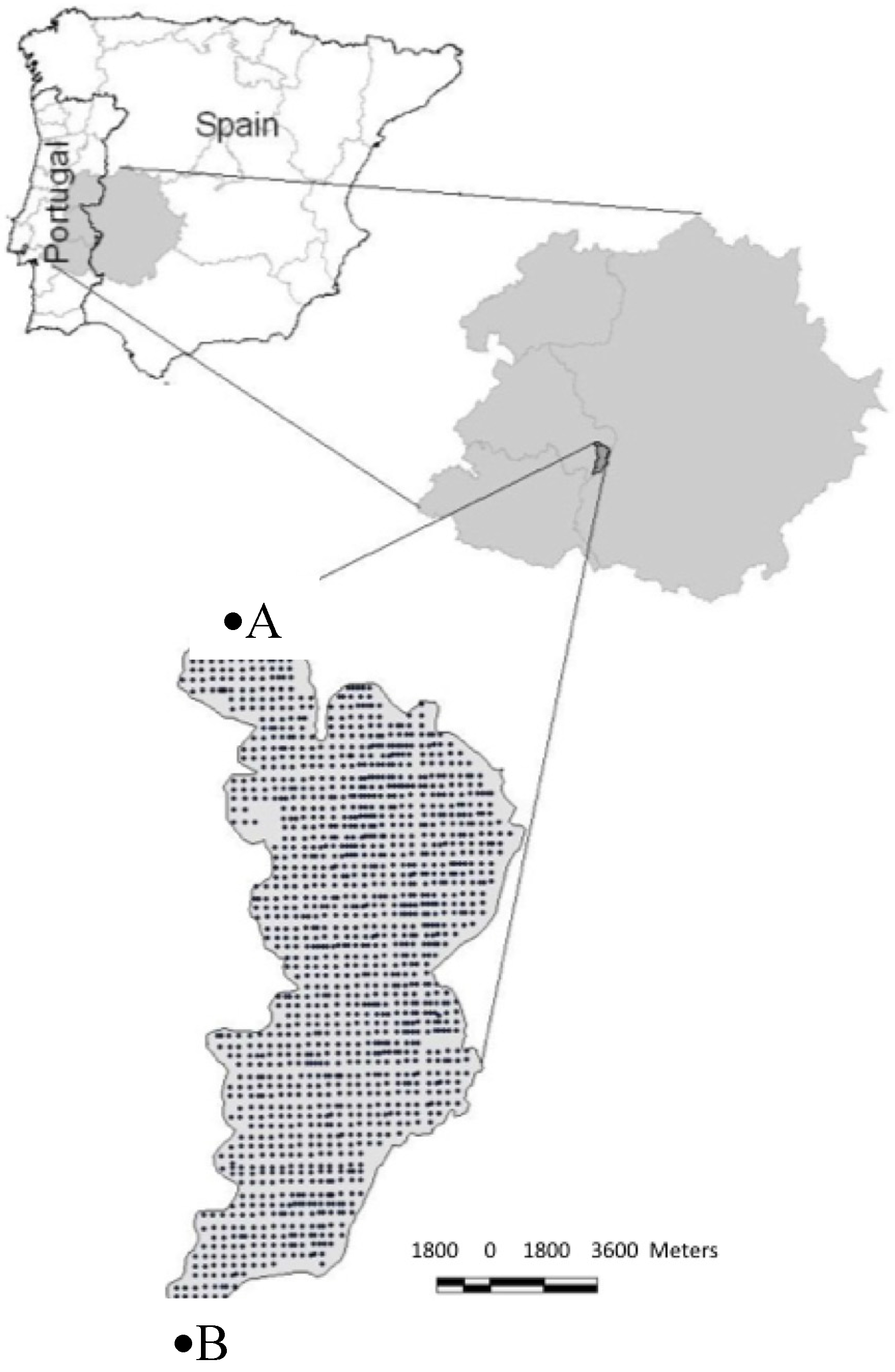
2.1. Study Area—Brief Characterization

Located in the municipalities of Elvas and Campo Maior, the study area is adjacent to the Portuguese-Spanish border at the confluence of the Rivers Caia and Guadiana, (Figure 1). Geologically the area is characterized mainly Cambrian and Silurian formations, presenting also some small sites with eruptive zones generally associated to hyper-alkaline and alkaline rocks [16].

Regarding climate, annually rainfall is approximately 483 mm, coinciding generally with the coldest temperatures in during autumn and winter. Maximum and minimum average temperatures range from 8.8 °C (in January) to 24.7 °C (in July). The most common productions are maize (almost half of the cultivated area), wheat (17%), sunflower (7%), tomato (6%), and olive trees (4%) [16].

In terms of relieve, one can find essentially very gentle slopes, mostly bellow 3% (around 80% of the study area), and between 3% and 5% (approximately 16%). The remaining areas which present slopes greater than 5% are not generally used for irrigated agriculture.

Regarding soil type (Portuguese classification): In the agricultural area covered by the Caia perimeter, the predominant soil types are Mediterranean soils (Figure 2 and Figure 3) from hydromorphic sandstones or clay conglomerates (Pag), occupying 36.1% of the total area, followed by Mediterranean soils of marl or limestones (Pac) with 10.8% of the total area. To these soil units, considered as the most representative, there are more than 10 other types of different soils, whose area is less than 4% of the total area of the perimeter.

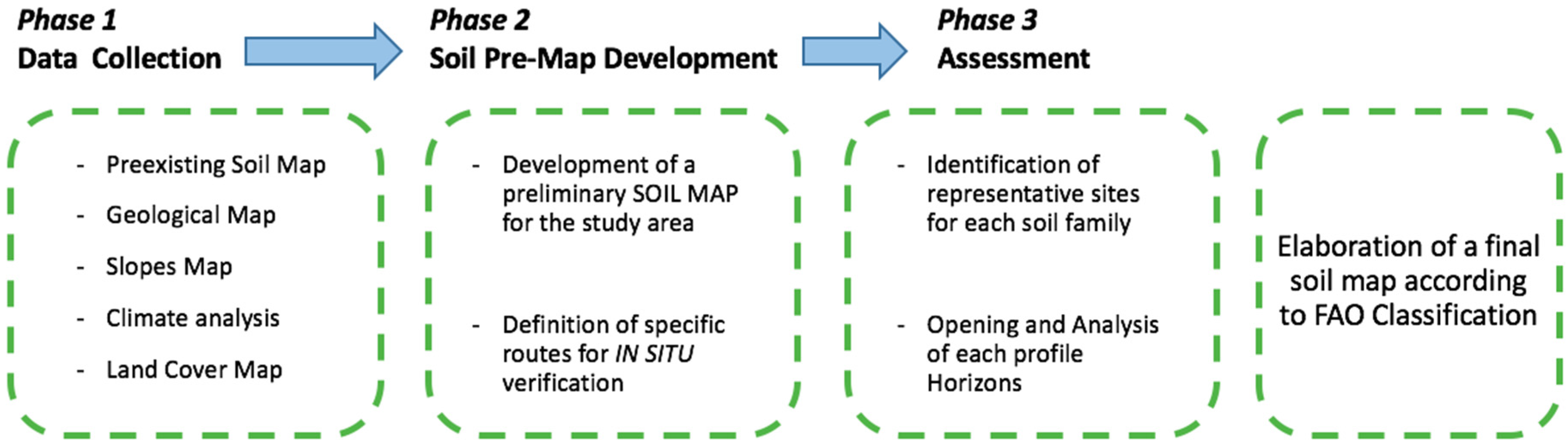
2.2. Used Methodology towards the Definitions of Soil Units

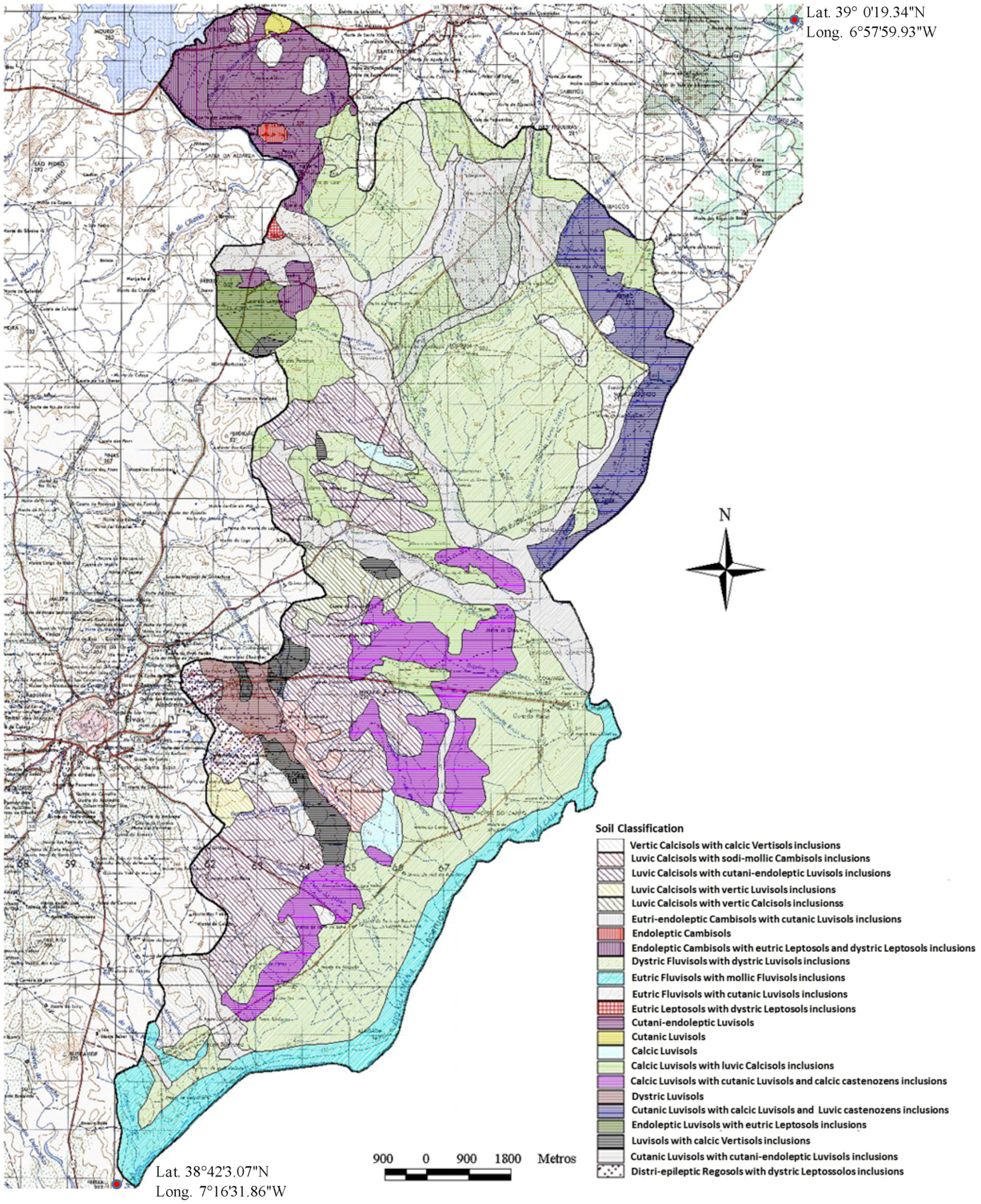
The methodology followed in the classification and soil mapping used a sequence of phases (Figure 4). First, a set of data was compiled, considering maps and other studies of the factors of soil formation in the area, including geology [17], climate, topography, and vegetation. The topographic data was obtained for analysis on-site, using a precision GPS (Global Position System) indicating altitude, which was then inserted in GIS software to generate the respective map (Figure 4).

This information allowed us to establish the routes and to understand the potential soil type in the area under study, providing the basis for the development of the required mapping. For the classification of different soil types we used the methodology recommended for WRBSR [18].

Then, a first field trip was held to establish contact with the study area and in order to plot on the map its limits. Based on the obtained field information and on the data previously collected from the aforementioned sources, a first preliminary map of the Caia Irrigation Perimeter was drawn.

In order to test the adjustment of this map to the geological reality of soils and geomorphology already mapped, a number of routes in the field, uniformly distributed, was planned, collecting samples in the different units, in order to establish both the type and variability of existing soils in each of the previously identified units.

Based on the previously described work and evidence, corrections and reinterpretations of the preliminary soil map were performed in order to promote the selections of the soils that, in our view, best represented soil diversity in terms of both a typological point of view and the soil properties.

For the characterization of the different soil types, we proceeded to survey of 26 soil profiles and their description, carried out according to the FAO Profile Description Guide [19] and to the Munsell Color Chart [20]. Samples of each of the horizons of different profiles were collected and, once properly packaged, labeled, cataloged, and then transported to the laboratory.

Regarding lab work, all the samples were air-dried. After this drying process, part of the sample was used in the determination of rough elements, while the remaining fraction of the sample was sieved through a stainless steel sieve with a 2 mm mesh.

The performed analyses were: particle size analysis—conducted by the method of Robinson pipette [21]; organic carbon—wet oxidation with potassium dichromate, followed by quantitative determination by titration with ferrous sulphate [21]; pH—potentiometry in a soil/water mixture (1:5 v/v); electrical conductivity—with a conductivimeter in an aqueous extract (1:5 v/v) under Rhoades [22]; total nitrogen—according to the Kjeldahl method [23]; phosphorus and potassium “assimilated”—according to the Egner–Riehm method [24]; calcium and magnesium—extracted with ammonium acetate buffered to pH 7 [21]; exchangeable bases and acidity—extraction with a barium chloride and triethanolamine solution buffered at pH 8.2—the Mehlich method [25]; extracting microelements (Cd, Cr, Cu, Fe, Mn, Ni, Pb, and Zn)—extracted with a solution of ammonium acetate, acetic acid, and EDTA—the Lakanen and Ervio method [26]; chlorides—extraction with water and assay by titration with silver nitrate—Mohr’s method [21]; and carbonates—dosed by a volumetric calcimeter using the Bernard method [27].

3. Results

As shown in

Table 1. Representation of reference units according to WRBSR (2006) at the Caia Irrigation Perimeter.

Soil Group	Area (ha)	Area (%)	Accumulated (%)
Leptosols	9	0.1	0.1
Regosols	150	1.2	1.3
Fluvisols	5640	44.9	46.2
Cambisols	693	5.5	51.7
Luvisols	3725	29.6	81.3
Calcisols	2342	18.7	100
TOTAL	12,549	100

, the area of the Caia Irrigation Perimeter has a significant diversity of soils. In Appendix, it is possible to assess 17 different profile descriptions, corresponding to 17 different soil types, which were obtained from the 26 analyzed profiles.

Considering the taxonomic levels, 23 different soil units were identified (

Table 2. WRBSR soil representation—soil type abundance at the study area.

Cartographic Units	Area (ha)	Area %
Eutric Leptosols with dystric Leptosols inclusions	9	0.1
Distri-epileptic Regosols with dystric Leptosols inclusions	150	1.1
Dystric Fluvisols with dystric Luvisols inclusions	3747	29.9
Eutric Fluvisols with mollic Fluvisols inclusions	703	5.6
Eutric Fluvisols with cutanic Luvisols inclusions	1190	9.5
Eutri-endoleptic Cambisols with cutanic Luvisols inclusions	458	3.7
Endoleptic Cambisols	18	0.2
Endoleptic Cambisols with eutric Leptosols and dystric Leptosols inclusions	207	1.6
Cutani-endoleptic Luvisols	506	4.0
Cutanic Luvisols	16	0.2
Calcic Luvisols	91	0.7
Calcic Luvisols with luvic Calcisols inclusions	997	8.0
Calcic Luvisols with cutanic Luvisols inclusions	889	7.1
Cutanic Luvisols with cutani-endoleptic Luvisols inclusions	93	0.7
Dystric Luvisols	154	1.2
Cutanic Luvisols with calcic Luvisols inclusions	601	4.8
Endoleptic Luvisols with eutric Leptosols inclusions	150	1.2
Luvisols with calcic Vertisols inclusions	228	1.8
Luvic Calcisols with vertic Calcisols inclusions	440	3.5
Luvic Calcisols with sodi-mollic Cambisols inclusions	158	1.3
Luvic Calcisols with cutani-endoleptic Luvisols inclusions	1497	11.9
Luvic Calcisols with vertic Luvisols inclusions	59	0.4
Vertic Calcisols with calcic Vertisols inclusions	188	1.5
TOTAL	12,549	100

and Figure 5); the Distric Fluvisols with Distric Luvisols inclusions was the most represented soil unit, occupying 29.9% of the total study area. The soils of the region, of which only 51.4% are regularly utilized in irrigation (the remaining area is rain-fed), are characterized by having good drainage conditions (90.7% soil good drainage), a medium to high depth (66.1% of soils have a useable depth greater than 1 m and 27.7% have a useful depth of between 50 and 100 cm), and low stone content (92.3% of stony soils have a lower 15%).

From a chemical point of view, these soils are mostly neutral to slightly alkaline (38.6% of the study area presents a pH between 6.0 and 7.0, and 38.3% have pH between 7.0 and 8.0), have low electrical conductivity (EC), probably the result of the good quality of the water used in irrigation (90.2% of the soils of this region have EC less than 0.25 dS·m⁻¹), are low in organic matter (66.2% of the soils have an organic matter content of less than 1.5% and only 6.9% had more than 2.0% of this important soil component), have a medium to high “assimilable” phosphorous content (73.5% soil this region have more than 100 mg·kg⁻¹ of P₂O₅), and have high to very high “assimilable” potassium content (94.4% of soils have more than 100 mg·kg⁻¹ “assimilable” potassium and 50.9% soils have more than 200 mg·kg⁻¹ “assimilable” potassium).

These soils are characterized by low carbonate content (74.8% of the soils of this region have between 0% and 25% CaCO₃) and high cation exchange capacity (CEC) (69.5% of the region’s soils have more than 10.0 cmol(+)·kg⁻¹ CEC, while for 12.2% of the region soils this value exceeds 20.0 cmol(+)·kg⁻¹ in which calcium is largely dominant). The percentage of exchangeable sodium is usually low, with 95% of the land area having less than 5% of exchangeable sodium.

Vulnerability to agricultural and environmental degradation is one of the most important problems in semi-arid regions around the Mediterranean basin.

During the development of the present research, we mapped several other characteristics of the soils of the study area. Based on this data and using GIS software, we were able to develop a soil vulnerability map for the Caia Irrigation Perimeter (Figure 6) considering the soils which continue to be irrigated. For the construction of this map, we considered as areas of high vulnerability those who meet all of the following conditions: percentage of exchangeable sodium > 10%; electrical conductivity (EC) > 0.5 dS·m⁻¹; and organic matter < 1%.

We considered mean vulnerability areas as the ones that had all of the following characteristics, and that have not been classified as highly vulnerable areas: percentage of sodium exchange > 7.5%; electrical conductivity (EC) > 0.5 dS·m⁻¹; and organic matter < 1.5%

4. Discussion

The area comprises mainly four soil groups, including Fluvisols, Luvisols, Calcisols and Cambisols, totaling 98.8% of the area under study. Of these, the first two groups comprise 74.6% of the study area, and Cambisols are the group with lower expression, representing only 5.4% of the area. There are other groups of soils whose representation is much reduced, particularly Leptosols with 0.1% of the total area and Regosols with 1.1% of the total area.

This result is typical of Mediterranean soils. The high diversity, coming from the genesis of these soils in geological and climatic terms, observed in this region can be found in any previous studies made in this region [9]. This result is of great importance, because different soil families have distinct characteristics, and those differences are very relevant to the decision not only between irrigated or rain-fed agriculture, but also among different types of irrigation considering the main goal to contribute to improve sustainability of Mediterranean irrigated agro-systems.

Comparing the types of soil of the study area presented in the Portuguese Soil Map at the scale of 1:50,000 (1961) with the Soil Map obtained in the present work, although the classification system used is different and therefore difficult to compare with any other classification system, it is possible to verify the existence of a substantially larger number of different classes in this study, confirming, as previously reported by Alexander & Afonso in 2007 [9], the limitations of the Portuguese Soil Map when further information with greater detail is needed.

The augmented number of subclasses in soil classification on our proposal on existing classification is, according to Alexander & Afonso [9] and Nunes et al. [1], an important added value, as it allows us to obtain a much more detailed information distinguishing different soil stains, whose different characteristics (texture, organic matter content, useful depth, existence of an Impermeable soil layer, etc.) lead to the implementation of different irrigation schemes and cultural operations, which enable an increase in the sustainability of these fragile agricultural systems. Concerning vulnerability, as can be seen in Figure 6, there are two zones of greatest vulnerability. One is located in the north-central part of the study area, and coincides with terrain bordering the River Caia. The other is in the southeastern part of the study area, and the west bank of the River Guadiana. The vulnerability to desertification in these two zones can be attributed to irrigation and the heavy use of fertilizers. A more detailed statistical study of the influence of irrigation in the agricultural and environmental degradation of these soils showed that 81.3% of the irrigated land has a high to medium risk of vulnerability, whereas only 25.9% of rain-fed area presents a high or medium vulnerability to degradation. This clearly showed that irrigation can be a major factor of soil degradation in this type of agro-system.

In fact, the obtained results are very important because they enable us to identify which areas can be irrigated without any environmental impact, which areas can be irrigated but with extra care in what quantity and quality of applied water regards, and areas where irrigation is not possible from an environmental point of view. This study conducted for the Caia Irrigation Perimeter can be spread to any other irrigation region in the Mediterranean basin, constituting a method of rapid and easy application towards the determination of vulnerable areas regarding environmental degradation due to irrigation practices.

The sustainability of the Caia Irrigation Perimeter, implemented four decades ago, is nowadays a matter of large concern, because in particular cases we have already found some areas with significant productivity losses. However, it is noteworthy that the water used in the irrigation area, also examined in the present study, is of very good quality, being classified by FAO as "unrestricted for irrigation", mainly because it was only after 40 years of continuous irrigation that important problems were deeply studied, as soil loss and erosion [28] started to appear. Nonetheless, this is not a general overview for new irrigation areas, in which the used water quality is substantially lower. The environmental degradation of these soils will occur much faster. Therefore, for these soils, the development of a vulnerability map, updated frequently, following this approach, can provide important information in order to enable decision-makers to develop suitability maps as the ones presented by Bathrellos et al. [29], and to take some protective measures for these agro-systems, thus ensuring their environmental and economic sustainability within the framework of rural and agricultural spatial environments [30,31] as well as promote regional innovation patterns.

5. Conclusions

The region under study presents a wide range of soils. The performed analysis enabled us not only to classify 23 different soil units according to WRBSR (2006), having a number of substantially higher soil units that shown in Portuguese Soil Map, but also to ascertain that preexisting information, e.g., soil and geological maps, can be very useful in solving known problems [32,33]. Focusing only on higher taxonomic levels, one can see that the dominant soil groups in the region are Fluvisols, occupying 44.9% of the total area, followed by Luvisols with 29.6% of the total area. These two groups of soils together with Calcisols represent more than 90% (93.2%) of the soils of the region under study.

Considering the data collected, it is possible to conclude that a substantial part of the study area’s soils is at high risk of degradation (40.3%), both due to the intrinsic characteristics of the soil, and to the fact that it is submitted to irrigation for a very long period, which in some areas has already reached 40 years. For this reason, a periodic monitoring to avoid potentially serious environmental problems is advisable. This contributes to the debate of regional intelligence [34] within the context of agriculture [35], where new combinatory methods that allow spatially explicit models to integrate local decision-making should be fostered [36,37,38].

References

1. Nunes, J.; Ramos-Miras, J.; Lopez-Piñeiro, A.; Loures, L.; Gil, C.; Coelho, J. Concentrations of Available Heavy Metals in Mediterranean Agricultural Soils and Their Relation with Some Soil Selected Properties: A Case Study in Typical Mediterranean Calcareous Soils. Sustainability 2014, 6, 9124–9138. [Google Scholar] [CrossRef]
2. Rossiter, D. Classification of urban and industrial soils in the world Reference Base for Soil Resources. J. Soils Sediments 2007, 5, 1–5. [Google Scholar] [CrossRef]
3. Hartemik, A. The use of soil classification in journal papers between 1975 and 2014. Geoderma Reg. 2015, 5, 127–139. [Google Scholar] [CrossRef]
4. Blume, P.; Brümmer, G.; Fliege, H.; Horn, R.; Kandeler, E.; Knabner, I.; Kretzschmar, R.; Stahr, K.; Wilke, B. Scheffer/Schachtschabel Soil Science; Springer-Verlag: Berlin, Germany; Heidelberg, Germany, 2016. [Google Scholar]
5. Bressiani, D.; Gassman, P.; Fernandes, J.; Garbossa, L.; Srinivasan, R. Review of Soil and Water Assessment Tool (SWAT) applications in Brazil: Challenges and prospects. Int. J. Agric Biol. Eng. 2015, 8, 9–35. [Google Scholar]
6. Junge, B.; Skowronek, A. Genesis, properties, classification and assessment of soils in central Benin, West Africa. Geoderma 2007, 139, 357–370. [Google Scholar] [CrossRef]
7. Amezketa, E.; Lersundi, J. Soil classification and salinity mapping for determining restoration potential of cropped riparian areas. Land Degrad. Dev. 2008, 19, 153–164. [Google Scholar] [CrossRef]
8. Figueiredo, T.; Fonseca, F.; Nunes, L. (Eds.) Proteção do Solo e Combate à Desertificação: Oportunidade para as Regiões Transfronteiriças; Instituto Politécnico de Bragança: Bragança, Portugal, 2015.
9. Alexandre, C.; Afonso, T. Cartografia de Solos à escala de exploração agrícola: Aplicação a um ensaio de olival. Rev. Ciênc. Agrár. 2007, 30, 17–32. [Google Scholar]
10. Mishra, B. Soil Science and Land Use Planning: Myth, Reality, Evidence and Challenge. EC Agric. 2015, 1, 140–148. [Google Scholar]
11. Mueller, L.; Sheudshen, A.; Eulenstein, F. Novel Methods for Monitoring and Managing Land and Water Resources in Siberia; Springer: Cham, Switzerland, 2016. [Google Scholar]
12. FAO. World Reference Base for Soil Resources 2006. A Framework for International Classification, Correlation and Communication; Word Soil Resources Report 103; IUSS-ISRIC-FAO: Rome, Italy, 2006. [Google Scholar]
13. Nachtergaele, F.; Spaargaren, O.; Deckers, J.; Ahrens, B. New developments in soil classification. World Reference Base for Soil Resources. Geoderma 2000, 96, 345–357. [Google Scholar] [CrossRef]
14. Pietsch, D.; Lucke, B. Soil substract classification and the FAO and World Reference Base system: Examples from Yemen and Jordan. Eur. J. Soil Sci. 2008, 59, 824–834. [Google Scholar] [CrossRef]
15. Brevika, E.; Calzolarib, C.; Millerc, B.; Pereira, P.; Kabalae, C.; Baumgartenf, A.; Jordáng, A. Soil mapping, classification, and modelling: History and future directions. Geoderma 2016, 264, 256–274. [Google Scholar] [CrossRef]
16. Nunes, J.; Loures, L.; Loures, A.; Piñeiro, A.; Albarran, A. Characterization and Soil Mapping of the Caia Irrigation Perimeter. Int. J. Geol. 2015, 9, 59–63. [Google Scholar]
17. Direcção Geral de Minas e Serviços Geológicos. Carta Geológica de Portugal à escala 1:50,000. In Direcção Geral de Minas e Serviços Geológicos; Carta no 37-A, 33-C e 33-D; Serviços Geológicos, Ed.; Instituto Geográfico e Cadastral: Lisboa, Portugal, 1969. [Google Scholar]
18. FAO. Guidelines for Soil Description, 4th ed.; Food and Agriculture Organization of the United Nations: Rome, Italy, 2006. [Google Scholar]
19. USDA—United State Department of Agriculture. Soil Survey Laboratory Methods Manual; Soil Survey Investigation Report No 42; Version 3.0; USDA: Washington, DC, USA, 1996; p. 692.
20. USDA—United State Department of Agriculture. Munsel Soil Color Charts. In U.S. Department Agriculture Handbook 18—Soil Servey Manual; Mcbeth Division of Kollmorgen Instruments Corporation, Ed.; USDA: Washington, DC, USA, 1994. [Google Scholar]
21. Nelson, D.; Sommers, L. Total C, organic C and organic metter. In Methods of Soil Analysis. Soil Science Society of America Book Series No 5, Part 3—Chemical Methods; Sparks, D.L., Page, A.L., Helmke, P.A., Loeppert, R.H., Soltanpour, P.N., Tabatabai, M.A., Johnston, C.T., Summer, M.E., Eds.; Soil Science Society of America—America Society of Agronomy Publ.: Madison, WI, USA, 1996. [Google Scholar]
22. Rhoades, J. Soluble salts. In Methods of Soil Analysis. Part 2. Chemical and Microbiological Properties, 2nd ed.; Page, A.L., Miller, R.H., Keeney, D.R., Eds.; Agronomy 9; American Society of Agronomy, Inc.: Madison, WI, USA, 1982; pp. 167–179. [Google Scholar]
23. Bremner, J.M. Nitrogen-Total. In Methods of Soil Analysis. Soil Science Society of America Book Series No 5, Part 3—Chemical Methods; Sparks, D.L., Page, A.L., Helmke, P.A., Loeppert, R.H., Soltanpour, P.N., Tabatabai, M.A., Johnston, C.T., Summer, M.E., Eds.; Soil Science Society of America—America Society of Agronomy Publ.: Madison, WI, USA, 1996; pp. 1085–1123. [Google Scholar]
24. Riehm. Die amoniuumlakatatessigsaure, method zur bestimung der leichtlos richen phosphorsaüre in karbonathatigen boden. Agrochimica 1958, 4, 47–65. [Google Scholar]
25. Mehlich, A. Determination of cation and anion exchange properties of soils. Soil Sci. 1948, 66, 429–445. [Google Scholar] [CrossRef]
26. Cottenie, A. Los análisis de suelos y plantas como base para formular recomendaciones sobre fertilizantes. In Boletin de Suelos de la FAO No 38/2; FAO: Rome, Italy, 1982; p. 116. [Google Scholar]
27. Albareda, J.M. Determinación de los Carbonatos en el Calcímetro de BERNARD; Comissión de métodos analíticos del Instituto Nacional de Edafologia: Madrid, Spain, 1974. [Google Scholar]
28. Rozos, D.; Skilodimou, H.D.; Loupasakis, C.; Bathrellos, G.D. Application of the revised universal soil loss equation model on landslide prevention. An example from N. Euboea (Evia) Island, Greece. Environ. Earth Sci. 2013, 70, 3255–3266. [Google Scholar] [CrossRef]
29. Bathrellos, G.D.; Gaki-Papanastassiou, K.; Skilodimou, H.D.; Skianis, G.A.; Chousianitis, K.G. Assessment of rural community and agricultural development using geomorphological—Geological factors and GIS in the Trikala prefecture (Central Greece). Stoch. Environ. Res. Risk Assess. 2013, 27, 573–588. [Google Scholar] [CrossRef]
30. Vaz, E.; Painho, M.; Nijkamp, P. Linking Agricultural Policies with Decision-Making: A Spatial Approach. Eur. Plan. Stud. 2015, 23, 733–745. [Google Scholar] [CrossRef]
31. Tayyebi, A.; Tayyebi, A.; Vaz, E.; Arsanjani, J.J.; Helbich, M. Analyzing crop change scenario with the SmartScape™ spatial decision support system. Land Use Policy 2016, 51, 41–53. [Google Scholar] [CrossRef]
32. Papadopoulou-Vrynioti, K.; Alexakis, D.; Bathrellos, G.D.; Skilodimou, H.D.; Vryniotis, D.; Vasiliades, E.; Gamvroula, D. Distribution of trace elements in stream sediments of Arta plain (western Hellas): The influence of geomorphological parameters. J. Geochem. Explor. 2013, 134, 17–26. [Google Scholar] [CrossRef]
33. Bathrellos, G.D.; Gaki-Papanastassiou, K.; Skilodimou, H.D.; Papanastassiou, D.; Chousianitis, K.G. Potential suitability for urban planning and industry development by using natural hazard maps and geological—Geomorphological parameters. Environ. Earth Sci. 2012, 66, 537–548. [Google Scholar] [CrossRef]
34. Vaz, E. The future of landscapes and habitats: The regional science contribution to the understanding of geographical space. Habitat. Int. 2016, 51, 70–78. [Google Scholar] [CrossRef]
35. Vaz, E.; De Noronha, T.; Nijkamp, P. Exploratory landscape metrics for agricultural sustainability. Agroecol. Sustain. Food Syst. 2014, 38, 92–108. [Google Scholar] [CrossRef]
36. Vaz, E.; de Noronha Vaz, T.; Galindo, P.V.; Nijkamp, P. Modelling innovation support systems for regional development-analysis of cluster structures in innovation in Portugal. Entrep. Reg. Dev. 2014, 26, 23–46. [Google Scholar] [CrossRef]
37. Vaz, E. Managing urban coastal areas through landscape metrics: An assessment of Mumbai's mangrove system. Ocean Coastal Manag. 2014, 98, 27–37. [Google Scholar] [CrossRef]
38. Vaz, E.; Cusimano, M.; Hernandez, T. Land use perception of self-reported health: Exploratory analysis of anthropogenic land use phenotypes. Land Use Policy 2015, 46, 232–240. [Google Scholar] [CrossRef]
Figure 1. Localization map of the area studied—developed by the authors. Coordinates: Point A—Lat. 38°59′50.89″N–Long. 7°9′1.36″W; Point B—Lat. 38°42′3.85″N–Long. 7°15′52.74″W. Adapted from Nunes et al., 2015 [16].
Sustainability 08 00368 g001
Figure 2. Examples of the appearance of dried red soil. Used by permission of Antonio López Piñeiro.
Sustainability 08 00368 g002
Figure 3. Examples of the appearance of dried brown soil. Used by permission of Antonio López Piñeiro.
Sustainability 08 00368 g003
Figure 4. Methodological diagram.
Sustainability 08 00368 g004
Figure 5. Soil map from the Caia Irrigation Perimeter. Adapted from Nunes et al., 2015 [16].
Sustainability 08 00368 g005
Figure 6. Soil vulnerability map for the Caia Irrigation Perimeter—developed by the authors.
Sustainability 08 00368 g006