Article

Development of an Adaptive Forecasting System: A Case Study of a PC Manufacturer in South Korea

1
Computer Integrated Manufacturing Group, Global Foundries Inc., 400 Stonebreak Road Extension, Malta, New York, NY 12020, USA
2
Department of System and Management Engineering, Kangwon National University, 1 Kangwondaehak-gil, Chuncheon 200-701, Korea
*
Author to whom correspondence should be addressed.
Sustainability 2016, 8(3), 263; https://doi.org/10.3390/su8030263
Submission received: 30 September 2015 / Revised: 22 February 2016 / Accepted: 7 March 2016 / Published: 10 March 2016

Abstract

:
We present a case study of the development of an adaptive forecasting system for a leading personal computer (PC) manufacturer in South Korea. It is widely accepted that demand forecasting for products with short product life cycles (PLCs) is difficult, and the PLC of a PC is generally very short. The firm has various types of products, and the volatile demand patterns differ by product. Moreover, we found that different departments have different requirements when it comes to the accuracy, point-of-time and range of the forecasts. We divide the demand forecasting process into three stages depending on the requirements and purposes. The systematic forecasting process is then introduced to improve the accuracy of demand forecasting and to meet the department-specific requirements. Moreover, a newly devised short-term forecasting method is presented, which utilizes the long-term forecasting results of the preceding stages. We evaluate our systematic forecasting methods based on actual sales data from the PC manufacturer, where our forecasting methods have been implemented.

1. Introduction

This study introduces a case study of quality improvements on the demand forecasting system of a leading personal computer (PC) manufacturer in South Korea. Accurate demand forecasting is important for sustaining the profitability of the firm. This is because the results of demand forecasting influence the firm in various ways, such as in strategy-setting and developing production plans. PC demand forecasting tends to be rather difficult, and the reasons for the difficulty can be largely divided into two categories. The first category of reasons is related to product characteristics. The product life cycle (PLC) of a PC is generally very short, and the short-term demand fluctuations occurring throughout the PLC are very large. The products of this firm were reported to have PLCs as short as 10 to 40 weeks. Moreover, this firm has a wide variety in its product line-up, and the demand patterns differ by product. The second category of reasons is related to factors within the firm. The requirement of the level of forecasting accuracy and the timing when forecasting data is needed are different, depending on whether the department is marketing, purchasing, or production. Moreover, the forecasting range also differs by department, from long-term forecasts of over 6 months to forecast data for periods as short as one day. Therefore, the personnel involved in demand forecasting face difficulties. Prior to applying the demand forecasting methods introduced by this study, the marketing manager relied on a simple regression model and experience to forecast demand for many kinds of products. Moreover, significant effort was required to amend the demand forecasts on a weekly basis, as there were numerous types of products being sold. Despite these efforts, the quality of demand forecasting, as indicated by its accuracy, required improvements as it did not meet expectations. As such, this study examines a systematic, higher-accuracy demand forecasting methodology that can overcome these difficulties and meet the requirements.
The purpose of this study is to improve the accuracy of demand forecasting. Furthermore, this study aims to develop a systematic demand forecasting methodology that can be applied across the firm to meet the department-specific requirements for demand forecasting. The requirements on the range and point-of-time of demand forecasting by department can be divided into three connected stages, as shown in Figure 1. First, through long-term demand forecasting prior to product launch, the demand for the entire PLC term is forecasted. The method of forecasting prior to launch depends on whether the product is new or a follow-up product. A follow-up product is a previously launched product that has undergone a slight change in its parts due to changes in technology. Since actual sales data exists for products with similar performance, demand forecasting can be performed based on this data. On the other hand, to forecast demand for newly developed products, the demand-forecasting manager chooses reference products from a list of previously launched products to use in demand forecasting. The forecast data at this stage is used for securing the raw materials and presenting reference data for capacity planning. The forecast data of this stage becomes the base line for demand forecasting throughout the entire PLC term, and is continuously updated in the subsequent stages. This is because PCs have a wide fluctuation of demand throughout the PLC and the forecasts may differ greatly compared to the previous long-term forecast value. Therefore, a reduction in the potential gap is necessary. The second stage involves amendments to the long-term demand forecasts through forecasting changes in long-term demand after the product launch. Based on the actual sales data after the launch, the forecast values indicating sales forecast after three weeks of the launch are amended. The result of the forecasting from this stage is mainly used for estimating the trend of the future demand after 3 weeks. Therefore, small short-term fluctuations are not reflected, and only the base line set in the first stage of forecasting is updated. The last stage is the short-term demand forecasting after the product launch. This involves reflecting the short-term demand fluctuation into the base line for the next 1–2 weeks. The forecast values of these 1–2 weeks significantly influence the decision on inventory levels, and are used to confirm the planned weekly production volume. Throughout the PLC, amendments to forecast values of long-term and short-term demand are completed on a weekly basis after the product launch. As such, this study defines three periods from before the launch of the PC to the end of the PLC, and deals with the development of new and improved demand forecasting methodologies to improve the forecasting accuracy for each stage.
This study is composed of the following sections. Section 2 examines the related literature. Section 3 deals with the staged demand-forecasting model of three stages, as was previously mentioned. Section 4 utilizes actual data to confirm its performance, and this study concludes with Section 5.

2. Literature Review

Traditional demand forecasting methods, such as smoothing, regression model, or time series analysis do not take PLC characteristics into consideration, and are difficult to apply to PC demand forecasting with a short PLC. Forecasting methods that consider the PLC are based on growth models such as logistic function, Gompertz curve, and Bass diffusion model. The comparison of the logistic function and Gompertz curve can be seen in Trappey and Wu [1]. Our study utilizes the Bass model [2], which despite being introduced over 50 years ago, is utilized widely in forecasting the demands of high-tech products such as large-screen televisions [3], mobile phones [4], microprocessor products [5], and renewal energy [6]. Our study is based on the Bass diffusion model in forecasting the long-term demand prior to product launch, which involves searching for a pattern in the product life cycle. This pattern is used as the base line in the subsequent demand forecasting processes. The demand forecasting of high-tech products, such as integrated circuits [7], with short PLCs is difficult because the demand volatility is high and the PLCs become shorter due to rapid innovation [8]. As such, the development of demand forecasting methodology for products with short PLC is very active. Wu et al. [9] analyzed the reasons behind the volatility for demand for semiconductor products with short PLCs, and identified products that provide an advanced warning of demand changes. Ingalls and Foote [8] and follow-up studies provide further insight to the forecast methodology for products with short PLCs. For accurate demand forecasting using the Bass diffusion model, reliable parameter estimates are necessary. On the estimation of the three key parameters in the Bass Model, refer to Boswijk and Franses [10], and Hong et al. [11]. Recently, Hong et al. [11] presented the new estimation method, which combines non-linear least square (NLS) and ordinary least square (OLS). However, estimating the key parameters for new products before the product launch is not that simple. This study utilizes the Bayesian updating method to adapt the parameters to the realized demand as follows.
As PCs have large fluctuations of demand within its PLC, the forecasted results using the Bass model may differ significantly after the product launch. Therefore, it becomes necessary to amend the results forecasted using the Bass model, and this study utilizes the following strategy. The forecasted result of the Bass model is set as the base line. While the base line itself is being amended in the long term, a new short-term forecasting method is developed and utilized in order to ensure higher-accuracy of the short-term forecast. The Bayesian model is used for long-term base line amendments, and this Bayesian model is used actively for demand forecasts of various types. Appropriate reviews can be found in Aytac and Wu [12,13], Yelland et al. [14], and Zhu and Thonemann [15]; this study utilizes the Bayesian updating method developed by Zhu and Thonemann [15]. Zhu and Thonemann [15] also forecast PC demand in a manner similar to this study, and assert that it is difficult to forecast the demand of recent products with short PLCs using the traditional demand forecasting methods (smoothing, linear regression model, and so on). This is because the traditional methods do not effectively reflect the characteristics of products with short PLCs. They have developed an adaptive Bayesian model-based demand forecasting methodology, which also deals with the inventory problem. The reason why this study is differentiated from Zhu and Thonemann [15], despite dealing with forecasting demands of PCs, is that this study has developed a highly accurate short-term demand forecasting method apart from the long-term demand forecasts. That is, we utilize the result of Zhu and Thonemann [15], and present a newly developed short-term forecasting method. Moreover, this study has developed a systematic methodology that can meet the requirements of various departments within the firm. Although specific forecasting techniques can be the best for each department, it is undesirable to choose individual forecasting techniques for the each of departments, if they cannot guarantee the consistency. The three-stage approach in the study is proposed to meet the forecasting requirements of all departments while the consistency of forecasting data is preserved, so that all of the departments can work under the same assumption in demand forecasting.

3. The Development of the Demand Forecasting System

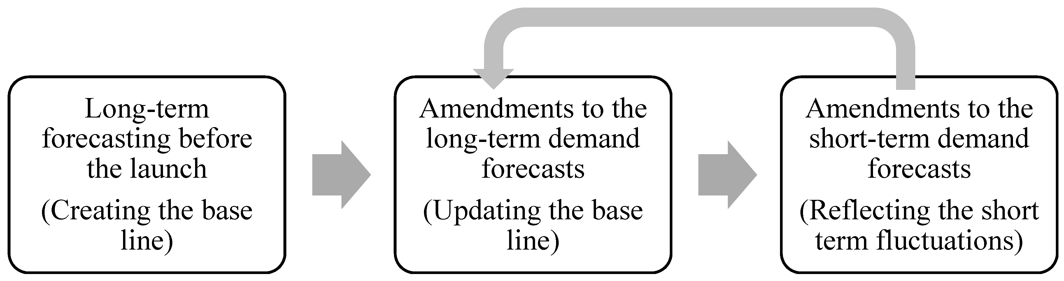
This section deals with forecasting demand by stage and amendment methods for the three stages of demand forecasting throughout the PLC. This is based on weekly forecasts, and daily forecasts are offered as reference points. The Bass diffusion model is used for forecasts.

3.1. Long-Term Demand Forecasting Prior to Product Launch

The purpose of this stage is to forecast the demand curve prior to product launch, which shows the entire demand pattern over the term of the PLC. The result of this stage is required by a production department to do capacity planning, a purchasing department to secure the raw materials, and so on. This stage goes through the following steps.
Step 1: Determine the planned sales volume and launch date of the new product.
Step 2: Select reference models.
Step 3: Analyze the past data of the selected reference models. Create and analyze the demand curve of the new product.
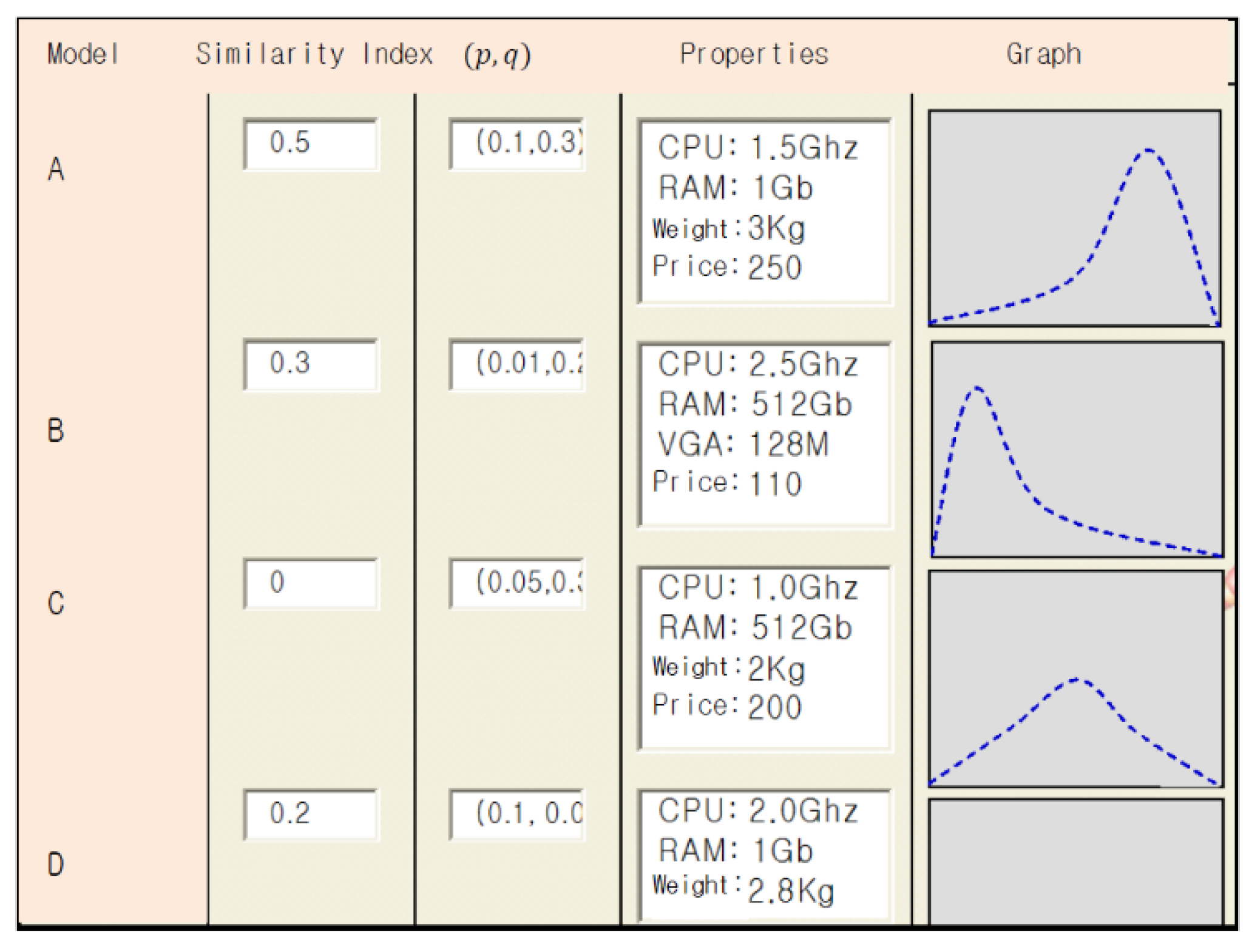
The method of selecting reference models in step 2 differs depending on whether the product is entirely new with no previous models, or builds on an existing product; the majority of products are of the latter kind. Suppose that the product to be launched is an entirely new product that differs completely from previous products. The demand-forecasting manager compares the characteristics of the new product with previous products, and selects reference models. Then, similarity index values for the selected reference models are assigned by the demand-forecasting manager. The similarity index values are distributed between 0 and 1, where the sum of all similarity index values is 1. Figure 2 shows a screen from the program developed to select reference models of new products. The product characteristics as shown in the “Properties” section are examined, and a number is assigned for the similarity index. Three products were selected in the example shown in Figure 2, and the sum of the similarity indexes is 1. At this point, ( p , q ) are parameters used in the Bass model where the cumulative demand by period t is denoted by:
N ( t ) = m 1 e ( p + q ) t 1 + q p e ( p + q ) t
where p indicates the coefficient of innovation (external influence) and q is the coefficient of imitation (internal influence), which are saved along with the product information. In other words, p indicates the extent of the influence of product-external factors on demand irrelevant to the product itself, such as the purchasing power of the consumer and market conditions. q indicates the extent of the influence of product-internal factors on demand such as product design and product pricing (Bass, 1969). m is the total number of people who will eventually use the product.
In Step 3, for the selected reference models in Step 2, the three parameters of the Bass model ( p , q , and m ) are estimated using their past sales data. Normally, firms possess the sales data for products that have been sold in the past few years. The sales of data of these products are fitted into the Bass model and the estimates for p , q , and m of previously sold products are saved in the database. These saved data are provided as a reference model to the user when demand is forecasted for the new product. These parameters go through the following stages to be estimated. First, any seasonal fluctuation in demand (seasonal effect) are removed from the past sales data of the selected reference models. X ( t ) indicates the actual sales data at a point of time in the past, t , while S ( t ) indicates a value where the seasonal effect is removed from X ( t ) . The seasonal coefficient at t can be represented by I ( t ) to yield the following well-known function to derive the sales data without the seasonal effects.
S ( t ) = X ( t ) I ( t )
Next, the Bass model is converted into a second-degree regression analysis. In the Equation (2) specified below, Y ( t ) indicates the cumulative sales records of the reference model up to the point t . f ( t ) 1 F ( t ) = p + q F ( t ) is the Bass model where f ( t ) is the change of the installed base fraction (i.e., f ( t ) d t is the probability of purchasing products), and F ( t ) ( = 0 t f ( u ) d u ) is the installed base fraction. Sales S ( t ) is the rate of change of installed base, which is f ( t ) multiplied by the ultimate market potential m . Cumulative sales Y ( t ) is the installed base fraction, which is F ( t ) multiplied by the ultimate market potential m . By replacing f ( t ) with S ( t ) / m , and replacing F ( t ) with Y ( t ) / m , we have:
S ( t ) = p m + ( q p ) Y ( t ) q m { Y ( t ) } 2
A regression analysis can be performed on the independent variable Y ( t ) and the response variable S ( t ) to yield a regression function, where the estimated intercept, the coefficient of Y ( t ) , and the coefficient of { Y ( t ) } 2 are called a , b , and c , respectively. Then, this function can be described as a = p m ,   b = q p , and c = q / m   , and the values of p , q , and m can be calculated by solving these equations. If estimation is completed using the p and q values from the regression analysis only, we have experienced that the model fit is not satisfactory regarding its accuracy. As such, we have devised a method where the value of m is held constant and p and q values are amended to increase the accuracy of the model. After obtaining the values of p and q using regression analysis, we applied an additional method. The method used is a simple search of a certain area, where the lower and upper values are set for p and q . The values of p and q are increased from their lower to upper values, which allows the determination of the values of p and q that minimize the sum of squared errors. 
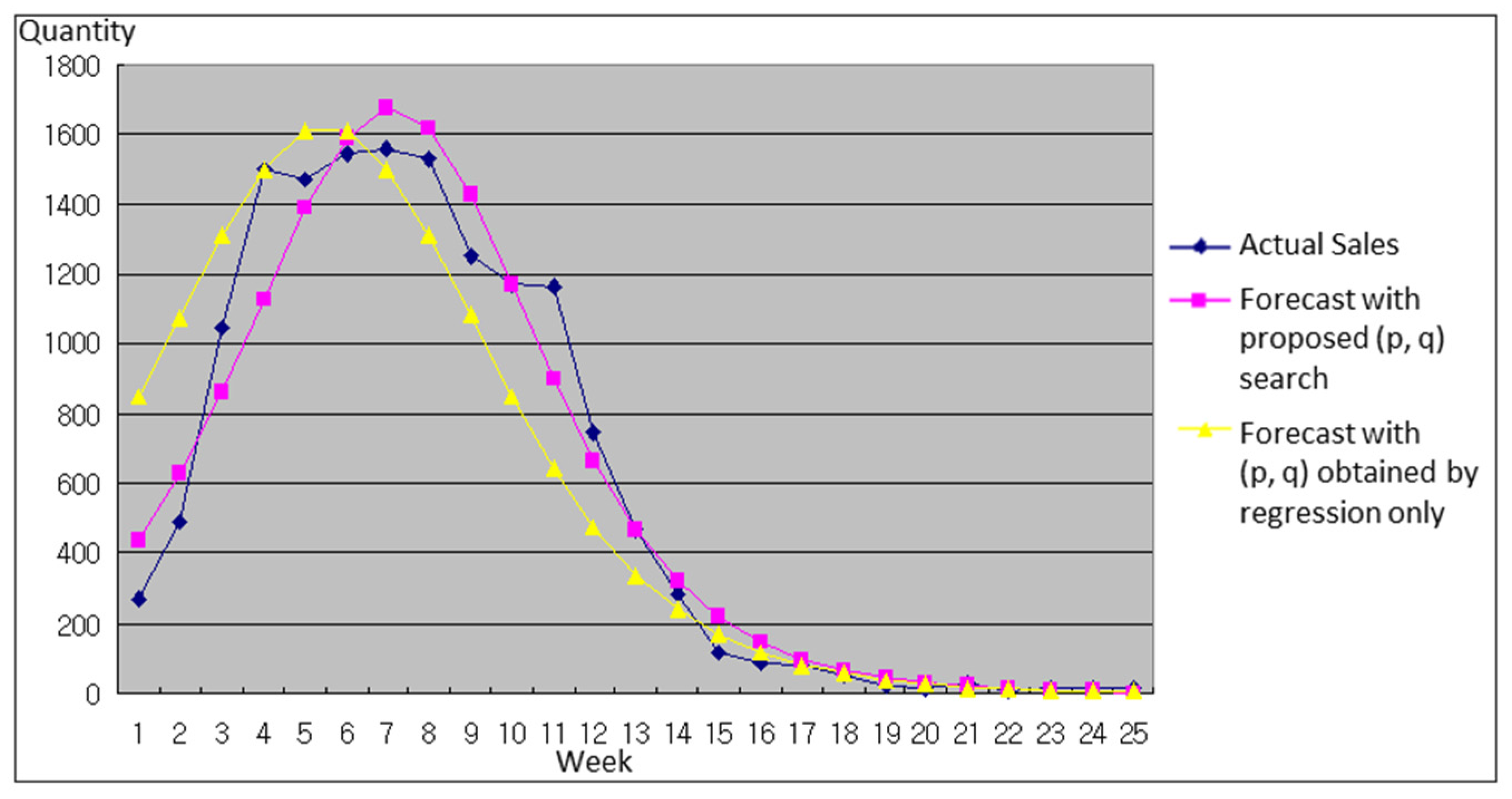
Figure 3 shows an example which compares two forecast results with the actual sales data. In this example, it can be found that forecasting using the values of p and q after additional search process results in improvement in model fit. At least, the error sum of squares after the additional search process cannot be increased when the additional searching process is applied.
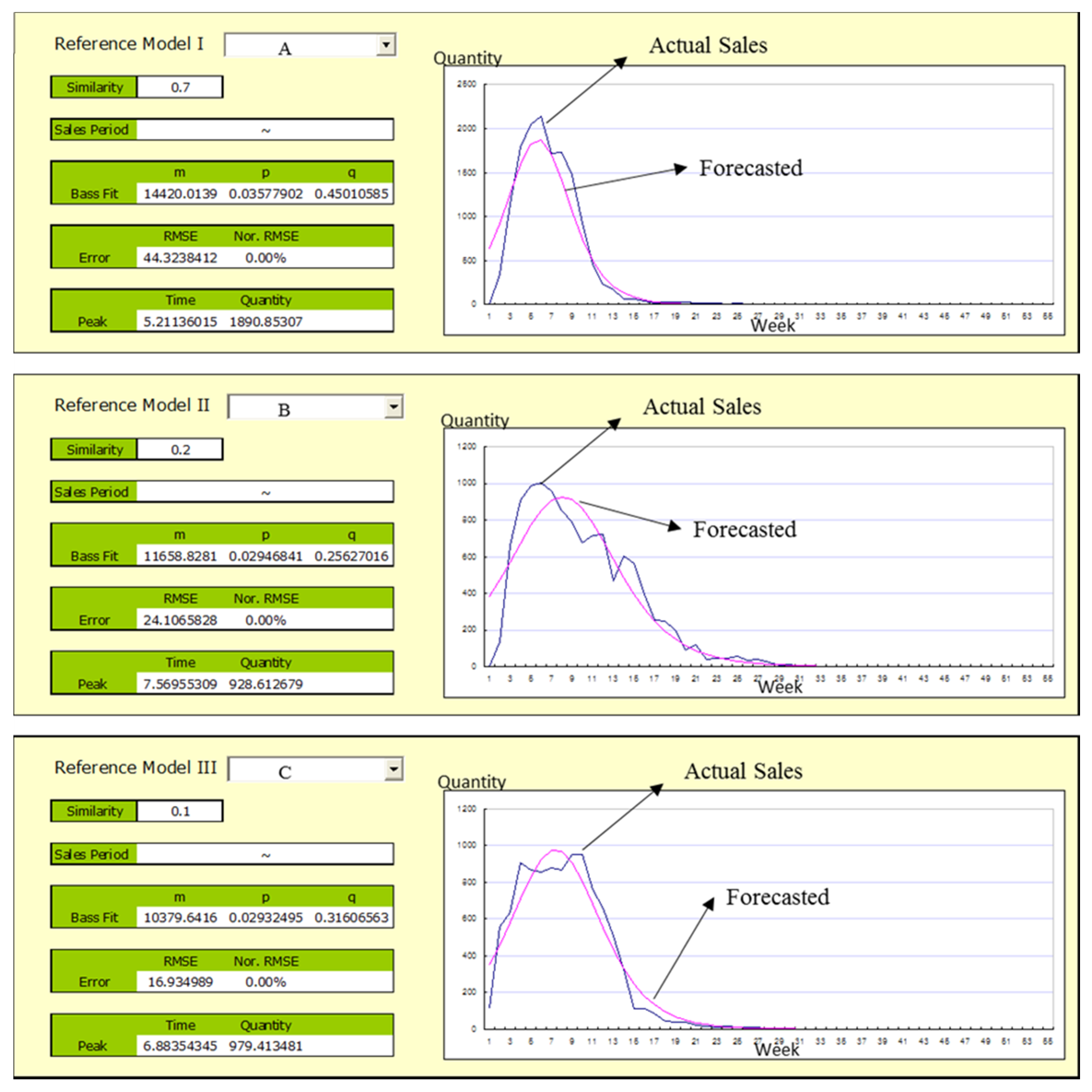
Figure 4 shows the results of estimating the parameters to be used for the new product, which are estimated by using the parameters of the selected reference models in step 2. The parameters p and q for the new product are estimated using the following function, and the m value is determined by the demand-forecasting manager.
p = i = 1 n s i p i ,   q = i = 1 n s i q i
In Equation (3), n is the number of selected reference models, s i , p i , and q i show the similarity index values of the i th reference model, and values of p and q . In other words, similarity index was utilized to calculate a weighted average. 
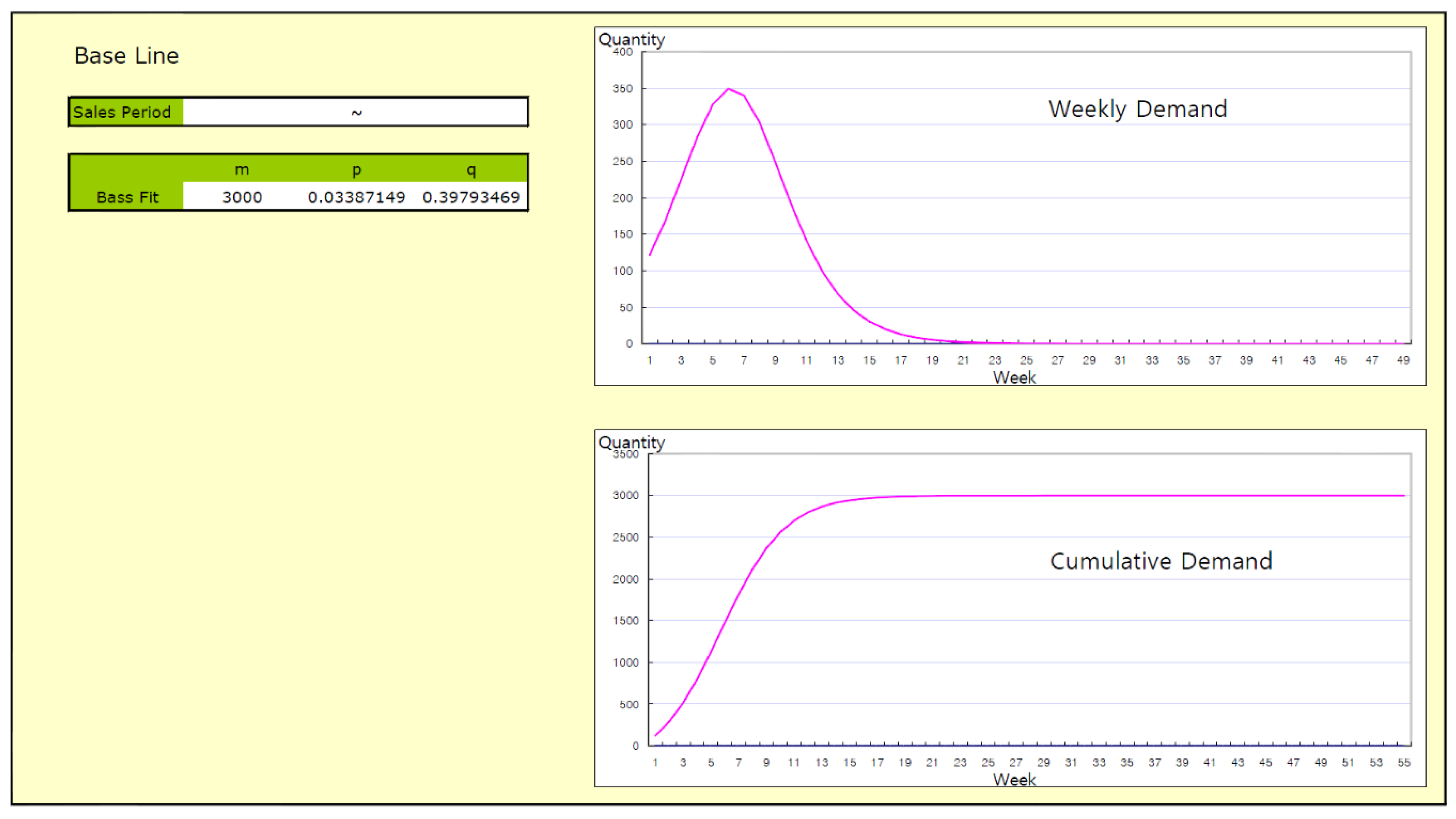
Figure 5 is an example of the generated demand curve (base line) for the new product. This curve is generated by using Equation (3). In this figure, the upper line shows a weekly demand forecast and the graph below indicates a cumulative graph.
The final demand-forecasting graph is used as the base line for short-term forecasting in the next stage, which is the product launch. After the launch, as new data are acquired, the base line is continuously amended for long-term forecasts. The drawn demand forecast graph can be analyzed to estimate the peak time where the sales volume is maximized (peak time t * ), and the maximum sales volume ( S ( t * ) ); these can be calculated using the following well-known equations in Bass [2] as well.
t * = ln q p p + q ,   S ( t * ) = m ( p + q ) 2 4 q

3.2. Amendments to Long-Term Demand Forecasts after Product Launch

At this stage, the base line that was formed in the forecast prior to launch is amended when actual sales data are gathered after product launch; these amendments are done 3 weeks after the launch, which is relatively long-term. Production related departments need the result of this second stage, with the improved accuracy than that of the first stage, to confirm the weekly production plan. The similarity index for the forecast prior to launch is a number between 0 and 1, and the values of the similarity index are amended at this stage. The updating method is based on the Bayesian updating method for the Bass diffusion model, suggested by Zhu and Thonemann [15]. This method is used to simultaneously update the parameters that determine the shape of demand forecasting curve, p , q , and m 
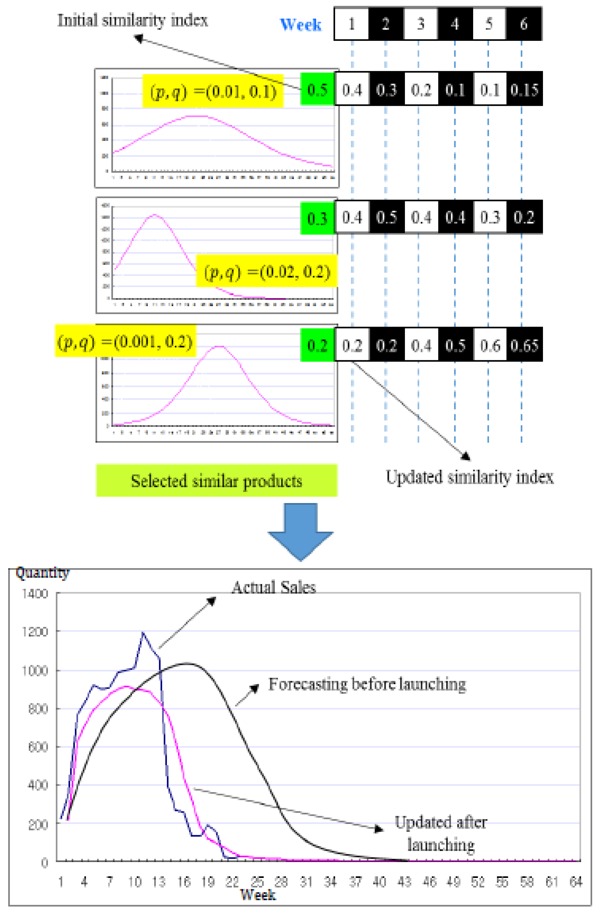
, which show the total sales volume. The example in Figure 6 shows three reference models, with initial similarity index values of 0.5, 0.3, and 0.2, respectively. These initial values were assigned by the marketing manager. Then, a week later the similarity index values are updated using the Equation (5). Suppose that the updated values of the three models are 0.4, 0.4, and 0.2, respectively. In this way, the values of the three models are updated to 0.15, 0.2, and 0.65 at week 6, respectively. Note that values in Figure 6 are arbitrarily chosen to illustrate the procedure. The performance of the updates can be seen in the picture below, and it can be seen that the data estimated using the updated p , q , and m are similar to the actual sales data. A comprehensive method of updating p and q is shown in Algorithm 1. A detailed calculation of the posterior probability in the Bass diffusion model can be found in Zhu and Thonemann [15].
Algorithm 1: Long-term forecast values amendment process.
Initialize1. Estimate the shape parameters of p and q of the Bass diffusion model for n number of selected reference models, and formulate n pairs of p i and q i , ( p i , q i ) ( 1 i n ) .
2. For each pair of ( p i , q i ) , define the prior probability Pr ( p i , q i ) and the prior distribution to sales ( m | p i , q i ) . The initial prior probability Pr ( p i , q i ) value is the initially estimated similarity index value.
3. t = 1
Repeat1. Calculate the posterior probability Pr ( p i , q i | X 1 , X 2 , , X t ) and posterior distribution ( m | p i , q i ) for each ( p i , q i ) and calculate the estimated sales volume. X t indicates the actual sales volume at week t .
2. t = t + 1
Until t T
According to Zhu and Thonemann [15], the posterior probability Pr ( p i ,   q i | X 1 , X 2 , , X t ) is calculated as follows.
Pr ( p i ,   q i | X 1 , X 2 , , X t ) =   w t ( p i , q i ) Pr ( p i , q i ) k = 1 n w t ( p k , q k ) Pr ( p k , q k )
where w t ( p i , q i ) is defined as:
w t ( p i , q i ) = τ t ( p i , q i ) j = 1 t s j ( p i , q i ) σ t ( p i , q i ) τ 0 ( p i , q i ) M 1 t ( p i , q i ) M 2 t ( p i , q i )
with
M 1 t ( p i , q i ) = exp { τ t 2 ( p i , q i ) 2 τ 0 2 ( p i , q i ) σ 2 ( p i , q i ) j = 1 t s j ( p i , q i ) [ X i s j ( p i , q i ) μ 0 ( p i , q i ) ] 2 }
and
M 2 t ( p i , q i ) = exp { τ t 2 ( p i , q i ) 2 σ 4 ( p i , q i ) j = 1 t k = 1 j 1 s j ( p i , q i ) s k ( p i , q i ) [ X i s j ( p i , q i ) X k s k ( p i , q i ) ] 2 }
and
τ t 2 ( p i , q i ) = τ 0 2 ( p i , p j ) σ 2 ( p i , q i ) S t ( p i , q i ) τ 0 2 ( p i , p j ) + σ 2 ( p i , q i )
s t ( p i , q i ) is the expected fraction of demand that occurs in period t and S t ( p i , q i ) = j = 1 t s j ( p i , q i ) μ 0 ( p i , q i ) and τ 0 2 ( p i , q i ) are the prior mean and the prior variance, respectively.

3.3. Amendments to Short-Term Demand Forecasts after Product Launch

Now, we present a newly developed forecasting method for short-term demand forecasts of 1–2 weeks using the actual sales data post-launch. While the previous sections have estimated and amended the demand patterns of the PLC of a product by utilizing well-known methods, this section aims to devise a novel method to reflect temporary increases or decreases in demand and to reduce the margins of error. This short-term demand forecast result with the higher fidelity is used to detect the change of sales pattern. The forecast method is based on the well-known Winter’s model, which is an extension of the linear exponential smoothing. When applied, it showed high accuracy for a product with relatively stable sales patterns.
A method of changing the Winter’s model to fit this study is explained below. Winter’s model is an appropriate forecasting method for products with long PLCs, and is not appropriate for products with short PLCs such as PCs, which is the focus of this study. As such, we developed a new short-term demand forecasting methodology by combining Winter’s model and the curve of the Bass diffusion model, which can be explained using the following pseudo code. Winter’s model reflects the randomness of demand, as well as the demand trend and seasonal effects. The trend in week t   is indicated by T t , and the seasonal effect is indicated by I t . I t is decided by the demand-forecasting manager beforehand. S t is a smoothed value where the seasonal effect has been removed, and X t is the actual sales volume in week t .
Algorithm 2: Short-term forecast for week T .
InitializeSet T 1 = 0.
Use the estimated value from the Bass curve (base line) for S 1 , i.e., S 1 = m 1 e ( p + q ) 1 + q p e ( p + q ) .
Set t = 2 .
Repeat S t = α ( X t I t ) + ( 1 α ) ( S t 1 + T t 1 )
L t = β ( S t S t 1 ) + ( 1 β ) T t 1
X t ' = X ( t ) = e ( p + q ) t m p ( p + q ) 3 ( p + e ( p + q ) t q ) ( p + e ( p + q ) t q ) 3  
T t = δ L t + ( 1 δ ) X t '
F t + l = ( S t + T t l ) I t + l
t = t + 1
Until t T
In the above pseudo-code, α , β , and δ are the adjustable parameters used in Winter’s model. We made a rule-of-thumb estimate for these values. The estimate value for the time ( t + l ) is shown as F t + l . X t ' = X ( t ) indicates the rate of change of base line at time t , which can be calculated by differentiating the Bass model. L t shows the rate of short-term demand change at the time t . The major difference between the original Winter’s model and ours is how to calculate trend factor T t 
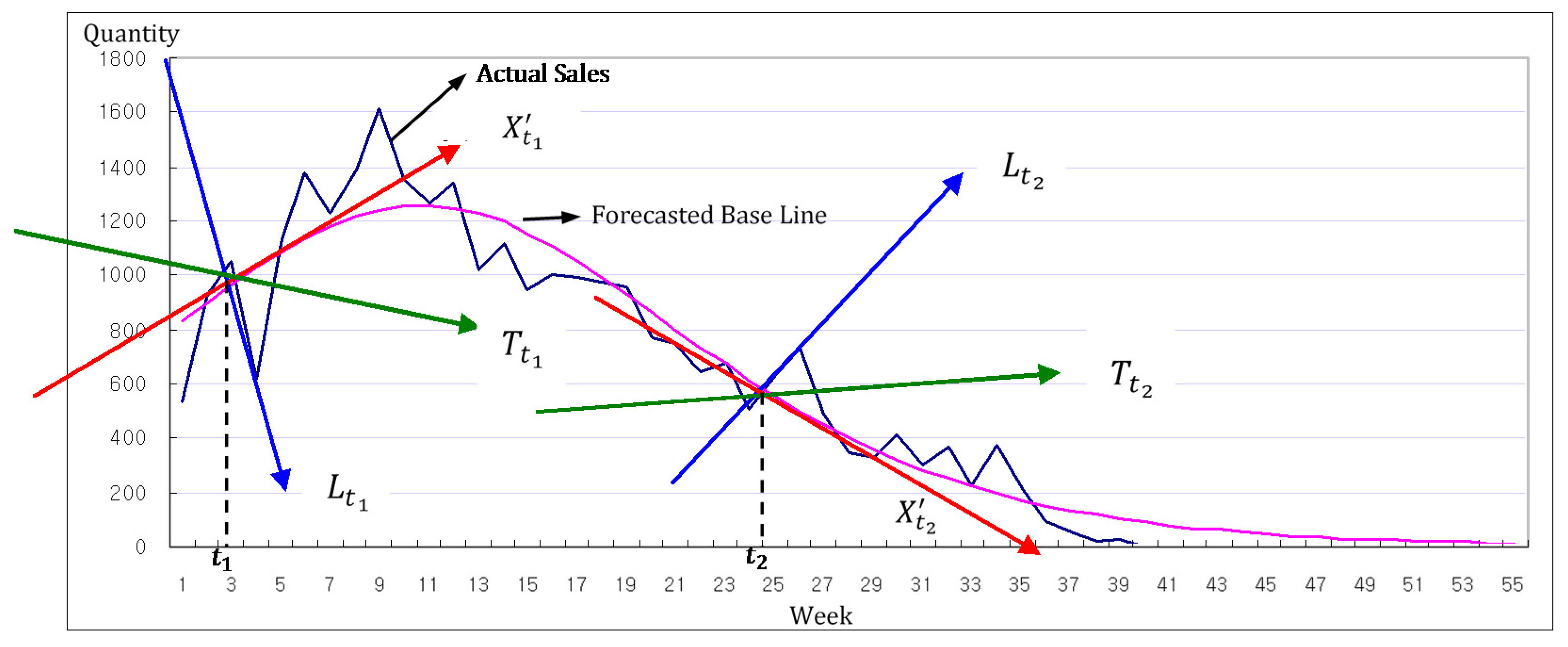
. The above method refines the trend factor using the slope vector of the Bass curve and reflects the trend more effectively. According to the definition of T t ,   T t is the composition of two trend factors (or vectors): short-term demand change at the time t (denoted by L t ) and the rate of change of PLC curve at the time t (denoted by X t ' ). In Figure 7, the compositions of two vectors are described at times t 1 and t 2 , respectively. By considering X t ' , when calculating T t , the long-term trend caused by PLC can be reflected in short-term forecasting. It improves the accuracy of forecasting.

4. Performance Assessment

This section tests the performance of the demand forecasting methodology suggested by this study using actual sales data. The products discussed are 37 products that have been launched in the past, which are comprised of 20 desktops and 17 laptops. Table 1 compares the accuracy of forecast between the method suggested by this study (shown as “This study”) and previous demand forecasting method used by the firm (shown as “in Use”). In case of desktops, the forecast accuracy was improved to 61% from 39%, and improved to 66% from 39% in case of laptops, which shows an increase that ranges between 1 percentage point (%P) and 54%P. Only one product showed decreased accuracy among the 37 products. On average, desktops showed an accuracy improvement of 22%P, while the accuracy improvement was 28%P for laptops. Based on a weighted average with respect to sales volumes, the overall accuracy was improved by approximately 15%P.
The suggested forecast methodology has a higher accuracy when the product has a higher sales volume. The only product with lower accuracy (desktop product number 18) has a low actual sales volume. When checked for weekly forecast accuracy, it was found that the forecasts were accurate in the weeks with higher sales.

5. Conclusion

This study deals with a case study where a systematic and highly accurate demand forecasting methodology is developed for PCs with short PLCs. The demand forecasting process was divided into three stages depending on the requirements and purposes. It utilized the well-known Bayesian updating methodology and a methodology that was developed throughout this study in stages. The demand forecasting methodology suggested in this study is more accurate than the previous methodologies used in the firm. In the third stage, a novel method for short-term forecasting is presented. It also allowed the satisfaction of requirements regarding terms and points of time for demand forecasting in various departments. Moreover, the verification of the methodology utilizing actual data showed large improvements in accuracy over previous demand forecasting methodologies used in the firm.
The demand forecasting system in this study has the following advantages. First, it has a higher accuracy compared to the forecasting method previously used in the firm. Moreover, it could satisfy various demands of different departments on the forecasting period and timing. As the demand forecasting methodology is implemented as a part of a software package and departments share the reference data using this program, demand forecasting could be done in a more systematic manner. Lastly, highly accurate demand forecasting can contribute to decreasing inventory.

Author Contributions

Chihyun Jung designed and performed this research, and developed a software package. Dae-Eun Lim collected and analyzed data. The majority of this paper is written by Dae-Eun Lim. All authors read and approved the final manuscript.

Conflicts of Interest

The authors declare no conflict of interest.

References

  1. Trappey, C.V.; Wu, H.-Y. An evaluation of the time-varying extended logistic, simple logistic, and Gompertz models for forecasting short product lifecycles. Adv. Eng. Inform. 2008, 22, 421–430. [Google Scholar] [CrossRef]
  2. Bass, F.M. A new product growth for model consumer durables. Manag. Sci. 1969, 15, 215–227. [Google Scholar] [CrossRef]
  3. Lee, J.; Cho, Y.; Lee, J.-D.; Lee, C.-Y. Forecasting future demand for large-screen television sets using conjoint analysis with diffusion model. Technol. Forecast. Soc. 2006, 73, 362–376. [Google Scholar] [CrossRef]
  4. Rui, H. Diffusion of mobile phones in China: application of Bass diffusion model. J. Converg. Inf. Technol. 2012, 7, 54–61. [Google Scholar]
  5. Wu, S.D.; Kempf, K.G.; Atan, M.O.; Aytac, B.; Shirodkar, S.A.; Mishra, A. Improving new-product forecasting at Intel corporation. Interfaces 2010, 40, 385–396. [Google Scholar] [CrossRef]
  6. Kumar, R.; Agarwala, A. Renewable energy technology diffusion model for techno-economics feasibility. Renew. Sustain. Energy Rev. 2016, 54, 1515–1524. [Google Scholar] [CrossRef]
  7. Hsu, L.-C.; Wang, C.-H. Forecasting the output of integrated circuit industry using a grey model improved by the Bayesian analysis. Technol. Forecast. Soc. 2007, 74, 843–853. [Google Scholar] [CrossRef]
  8. Ingalls, R.G.; Foote, B.L. Control-based life-cycle forecasting. IEEE Trans. Electron. Pack. 2003, 26, 5–13. [Google Scholar] [CrossRef]
  9. Wu, S.D.; Aytac, B.; Berger, R.T.; Armbruster, C.A. Managing short life-cycle technology products for Agere systems. Interfaces 2006, 36, 234–247. [Google Scholar] [CrossRef]
  10. Boswijk, H.P.; Franses, P.H. On the econometrics of the Bass diffusion model. J. Bus. Econ. Stat. 2005, 23, 255–268. [Google Scholar] [CrossRef]
  11. Hong, J.; Koo, H.; Kim, T. Easy, reliable method for mid-term demand forecasting based on the Bass model: A hybrid approach of NLS and OLS. Eur. J. Oper. Res. 2016, 248, 681–690. [Google Scholar] [CrossRef]
  12. Aytac, B.; Wu, S.D. Modelling high-tech product life cycles with short-term demand information: A case study. J. Oper. Res. Soc. 2011, 62, 425–432. [Google Scholar] [CrossRef]
  13. Aytac, B.; Wu, S.D. Characterization of demand for short life-cycle technology products. Ann. Oper. Res. 2013, 203, 255–277. [Google Scholar] [CrossRef]
  14. Yelland, P.M.; Kim, S.; Stratulate, R. A Bayesian model for sales forecasting at Sun Microsystems. Interfaces 2010, 40, 118–129. [Google Scholar] [CrossRef]
  15. Zhu, K.; Thonemann, U.W. An adaptive forecasting algorithm and inventory policy for products with short life cycles. Nav. Res. Logist. 2004, 51, 633–653. [Google Scholar] [CrossRef]
Figure 1. The three stages of demand forecasting.
Sustainability 08 00263 g001
Figure 2. Interface for selecting reference models.
Sustainability 08 00263 g002
Figure 3. Demand forecasting results after parameter estimation.
Sustainability 08 00263 g003
Figure 4. Example of the result screen for analysis of selected reference models.
Sustainability 08 00263 g004
Figure 5. Demand forecasting curve of created new product.
Sustainability 08 00263 g005
Figure 6. Performance improvement examples after update.
Sustainability 08 00263 g006
Figure 7. Three vectors X t ' ,    L t and T t .
Sustainability 08 00263 g007
Table 1. Performance comparison of forecasting methods in use and in this study.
TypeModel No.Accuracy of MethodTypeModel No.Accuracy of Method
in UseThis Studyin UseThis study
Desktop163%79%Laptop149%69%
265%76%210%64%
320%64%351%69%
414%63%437%64%
553%72%539%62%
653%75%635%78%
758%59%730%57%
834%75%849%75%
941%68%933%63%
1045%74%1067%76%
1114%68%1151%60%
1233%45%1228%66%
1337%54%1323%69%
1425%50%1434%69%
1548%58%1540%46%
1628%38%1632%67%
1733%44%1731%68%
1849%38%Average38%66%
1942%66%Forecast accuracy ( % )
= i = 1 T ( 1 F o r e c a s t   f o r   w e e k   i a c t u a l   s a l e s   i n   w e e k   i F o r e c a s t   f o r   w e e k   i ) × 100
2029%61%
Average39%61%

