The previous research on supply chains has mostly considered only one product and one manufacturing center, as Shukla
et al. (2011) [
18] do. This design does not fit the reality, and thus this paper considers supply chains with multiple products and manufacturing centers. The majority of enterprises have manufacturing centers for their products, delivering goods to their distribution centers and client regions where goods are in demand, and the three-echelon model has been adopted by many researchers (Shukla
et al., 2011; Meepetchdee and Shah, 2007; Peng
et al., 2011) [
18,
19,
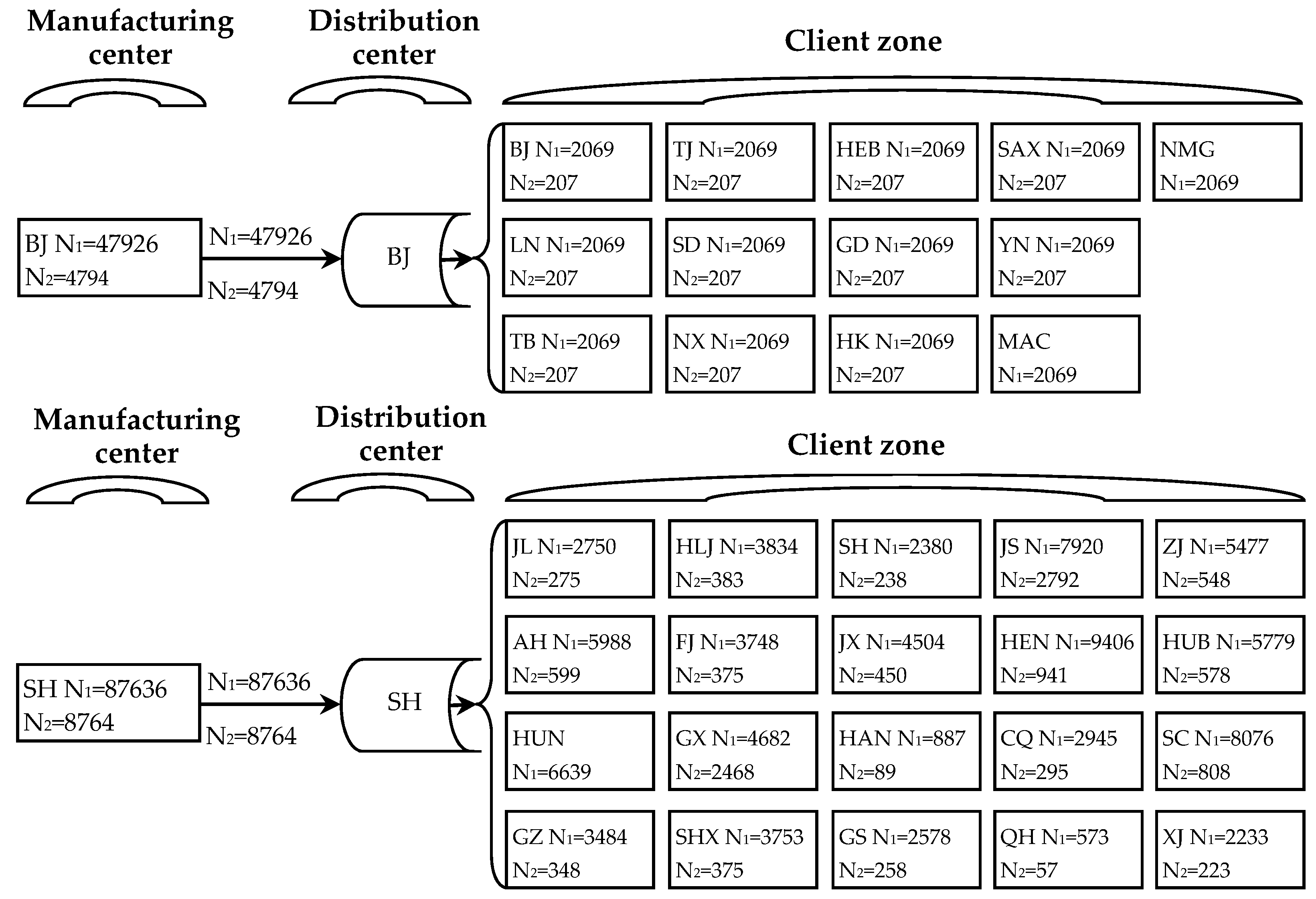
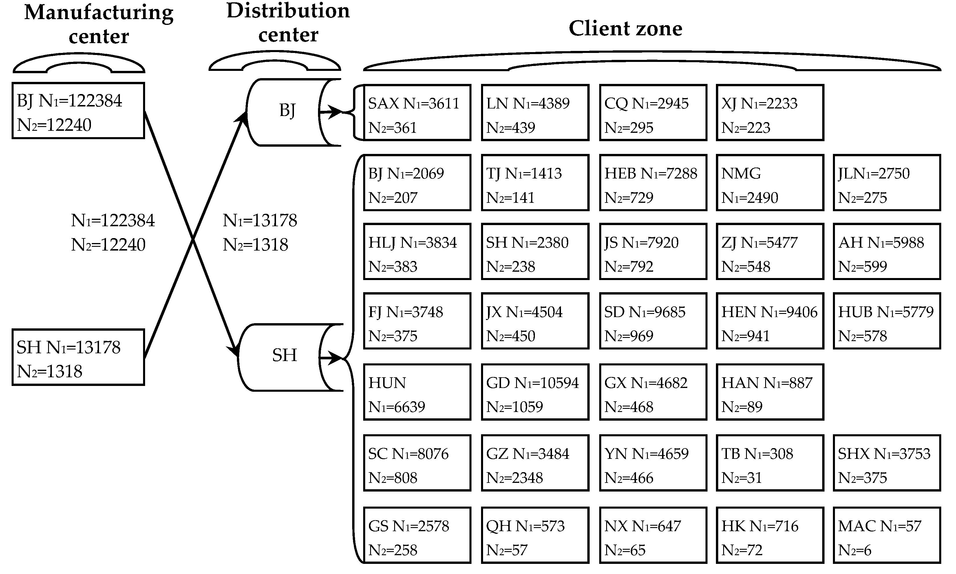
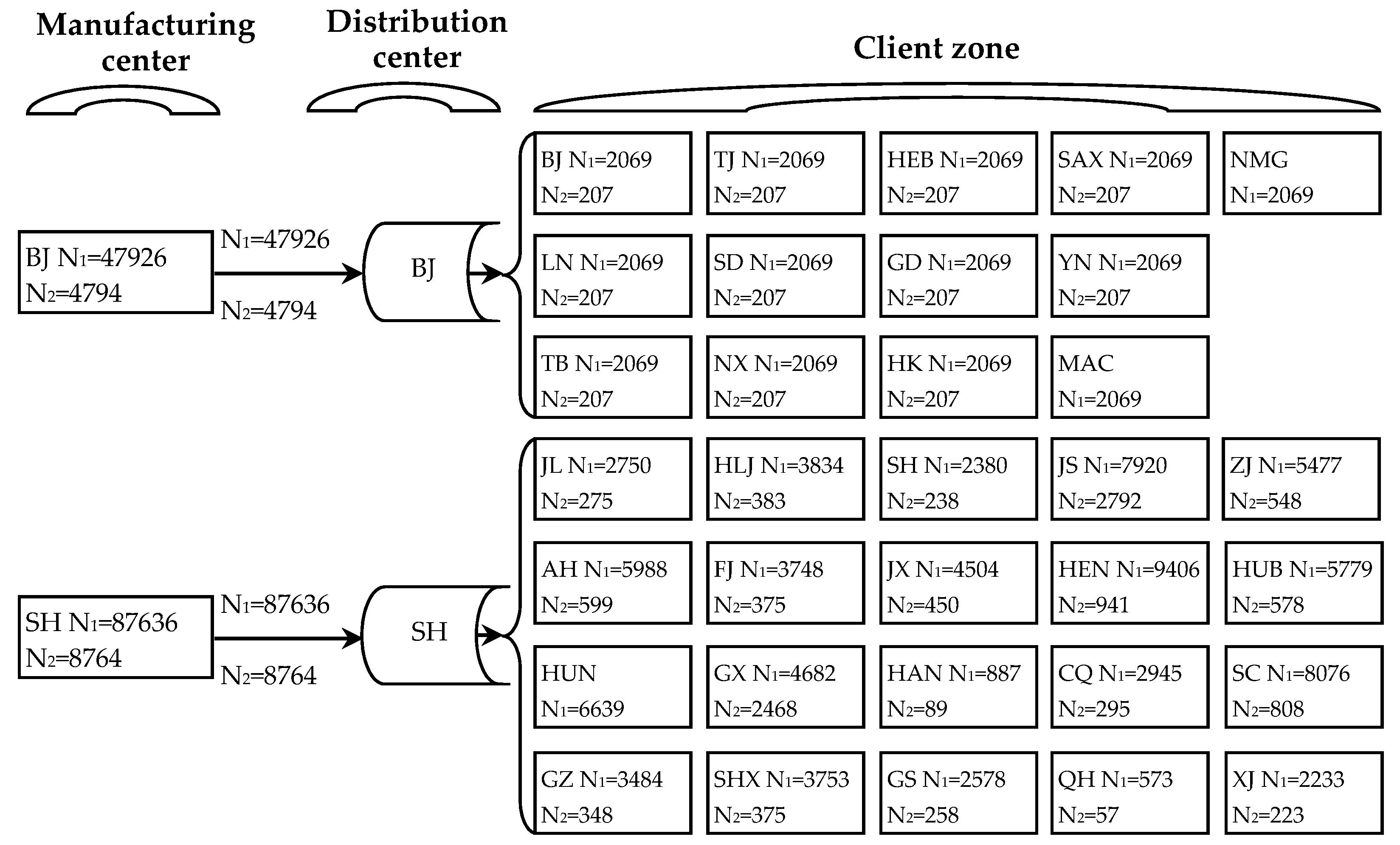
20]. As a result, this paper designs the three-echelon model with multiple products and manufacturing centers. The supply chain comprises the fixed manufacturing centers
a with multiple products, the potential distribution centers
b and fixed client zones
c, as shown in
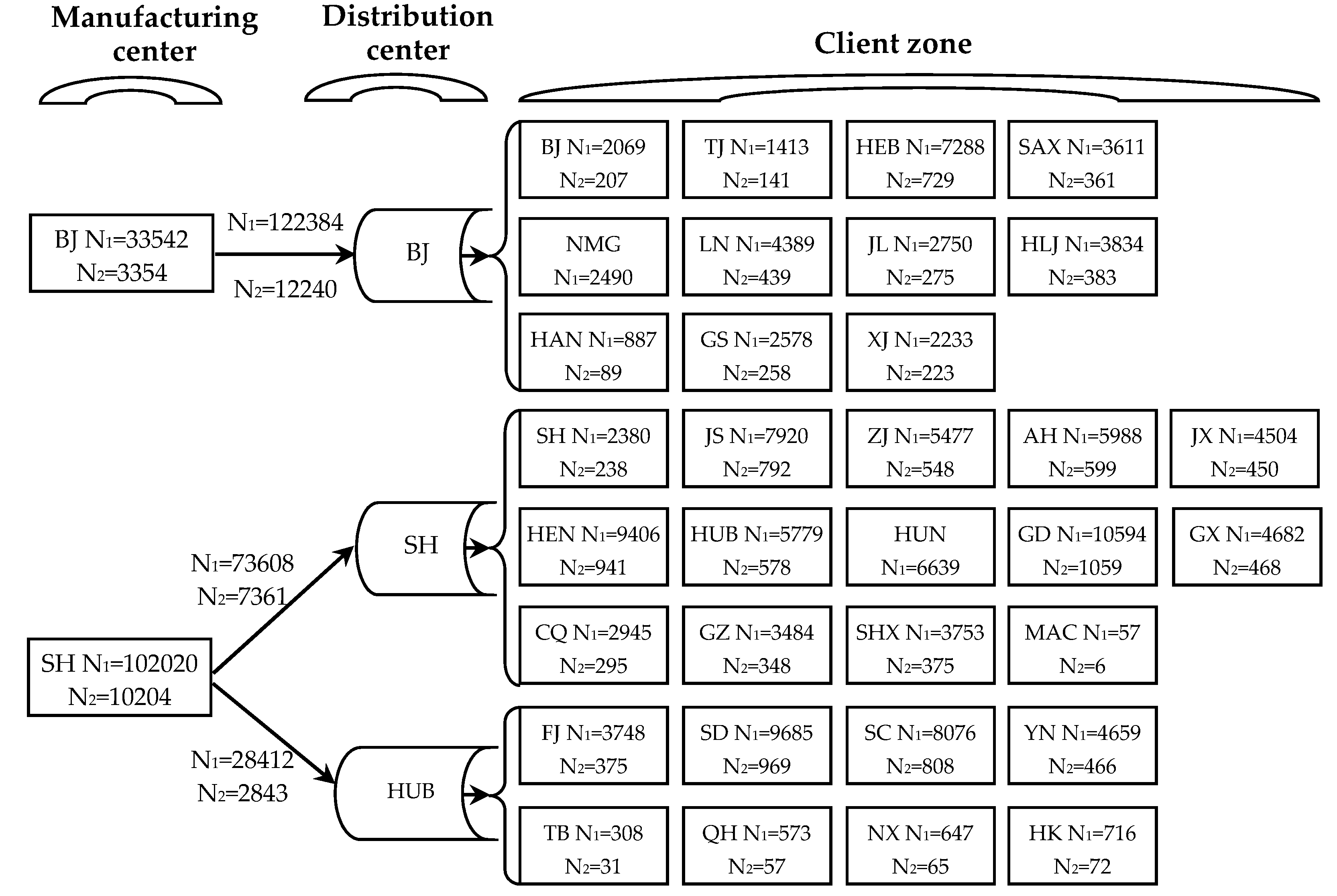
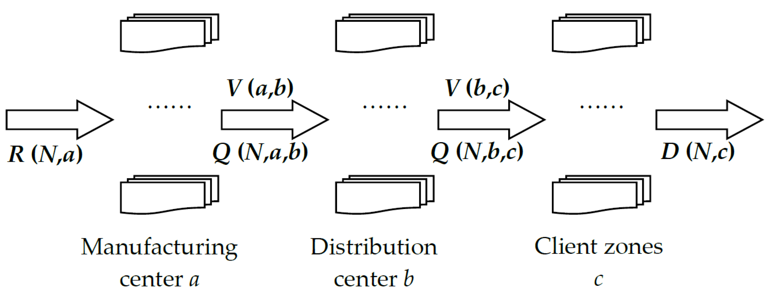
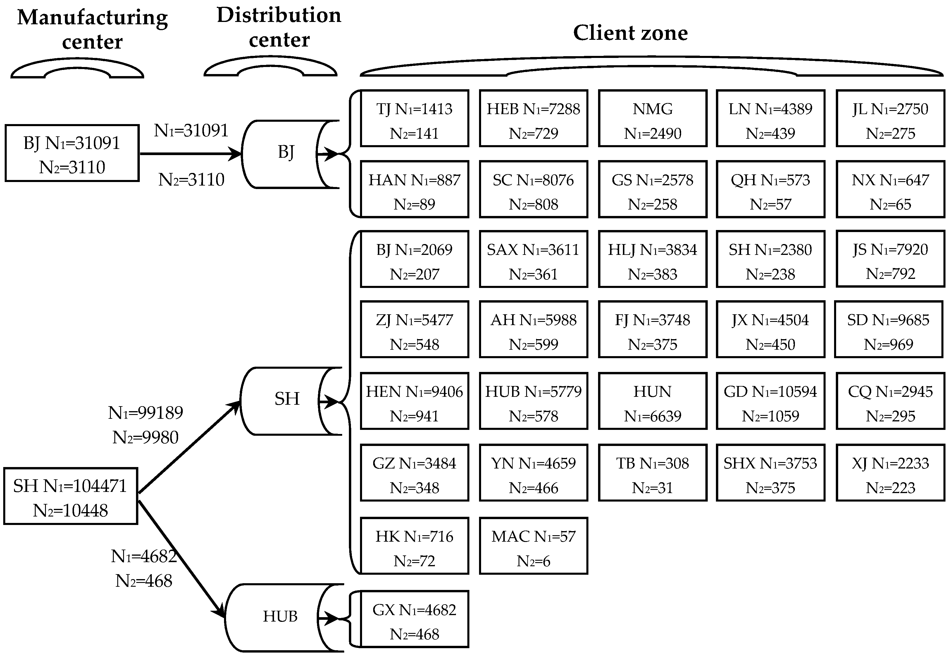
Figure 1. In this supply chain, the varieties and quantities of products in multiple manufacturing centers rest on the model; the numbers, locations, varieties and quantities of delivered goods depend on the model; and the construction of the distribution center leads to the corresponding cost of the infrastructure. The client zone represents the demand for one or multiple products. The operational cost includes infrastructure cost, manufacturing cost and material carrying cost in distribution centers and transport cost. The scenario planning is adopted to calculate and analyze the anticipated disruption cost in different cases of supply chain disruption. The scenarios can be the node disruption in the manufacturing center or distribution center, or the link disruption from manufacturing center to the distribution center or from distribution center to the client zone. To ensure stable operations in the overall supply chain system, once the distribution center is constructed, it must serve some client zones. Each distribution center and each client zone can be supplied by only one manufacturing center and one distribution center. There is no inventory accumulation or loss. The demand of each client zone can be satisfied. The data given consist of the demand of client zones, cost, manufacturing center and the distance between distribution centers and client zones, the probability of disruption in each scenario and the quantity of disrupted products. The aim is to maximize the two conflicting targets of efficiency and robustness of supply chains, and weigh and analyze efficiency and robustness and compare the total cost at the same time.
2.1. Parameters Setting
: manufacturing centers; : distribution centers; : client zones; : product types; : scenario collections.
Define whether manufacturing centers supply distribution centers as the binary system variables.
Define whether distribution centers supply client zones as the binary system variables.
Define the description of multi-echelon supply chains as integer variables.
: quantity of product by the manufacturing center ; : quantity of product from the manufacturing center to the distribution cente ; : quantity of product from the distribution center to the client zone .
: annual demand of the product in client zone .
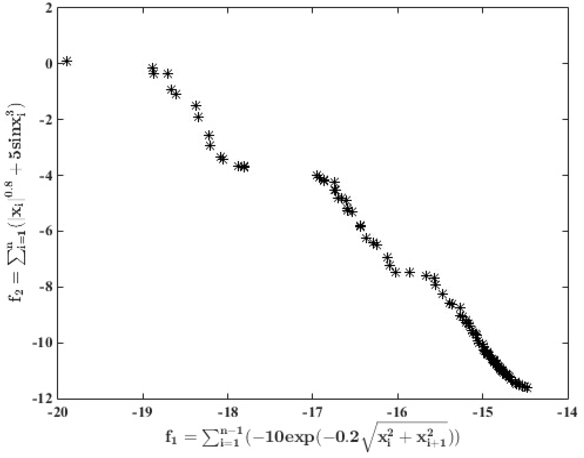
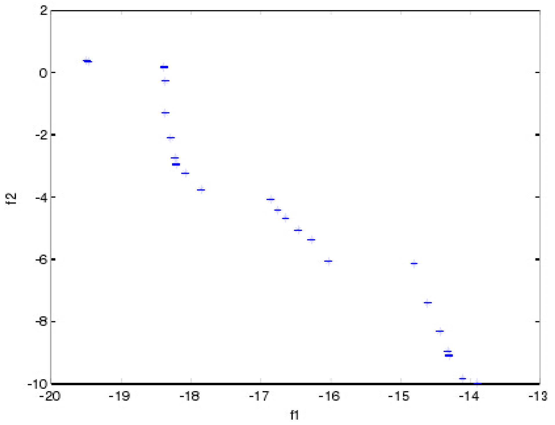
: efficiency of supply chains; : robustness of supply chains
: the fixed cost amortized annually when distribution center is constructed; : the unit changeable cost of product amortized annually when the distribution center is constructed; : the production cost of the unit product in the manufacturing center ; : unit carrying cost of the product in the distribution center ; : unit shipment cost of the unit product from the manufacturing center to the distribution center ; : the unit shipment cost of the unit product from the distribution center to the client zone ; : opportunity cost, i.e., unit marginal profit of Product .
: the distance from the manufacturing center to the distribution center ; : the distance from the distribution center to the client zone .
: probability of scenario
: quantity of disrupted product in scenario
2.2. Constraints
All the relevant network structure constraints in the manufacturing center, the distribution center and the client zone can be summarized as follows.
Formula (1) shows that if the manufacturing center serves distribution center , then the distribution center supplies at least some client zone. Formula (2) shows that if the distribution center is built, then the client zone may or may not be supplied by distribution center . As long as manufacturing center supplies distribution center , manufacturing center can provide distribution center with product . Thus, constraint (3) is formed, and is the appropriate large number, with k = 1,000,000,000. The same constraint can be applied to distribution center and the client zone , as shown in Formula (4). Formulas (5) and (6) are constraints with a single source to ensure that each distribution center and each client zone can be supplied by one manufacturing center and one distribution center.
If there is no inventory accumulation and loss, the material balance constraint can be summarized as follows.
Formula (7) shows that the quantity of product from manufacturing center to the distribution center amounts to the quantity of product in manufacturing center . Likewise, the quantity of product from manufacturing center to distribution center amounts to the quantity of product from distribution center to client zone , as shown in Formula (8). Formula (9) ensures that the demand of each client zone can be satisfied.
All the consecutive variables must be non-negativity.
To reduce the search space efficiently, efficiency and robustness of supply chains must be non-negative.
2.3. Objective Functions
The construction of supply chain considers efficiency and robustness, and thus the objective targets are defined as the two conflicting targets of the maximal efficiency and robustness. The efficiency of supply chains is expounded in terms of operational cost, whereas robustness of supply chains is explicated in terms of the anticipated disruption cost.
: the operations cost in most robust supply chains; : the operations cost in the most effective supply chains; : the anticipated disruption cost in the most robust supply chains; : the anticipated disruption cost in the most effective supply chains.
The operations cost of the objective functions include the infrastructure cost, production cost, the material carrying cost and shipment cost in the distribution center.
Formula (17) is the infrastructure cost incurred for the construction of the distribution center, which is a fixed cost. However, the changeable cost is the annual amortization, related to the unit changeable cost of product in the distribution center, multiplied by the quantity. If the production cost in the manufacturing center is in proportion to the quantity of products, the total production cost in the manufacturing center is as shown in Formula (18). Formula (19) shows that the material carrying cost in the distribution center is in proportion to the total handling capacity of the distribution center. Formulas (20) and (21) show the shipment cost from the manufacturing center to the distribution center, and from the distribution center to the client zone, respectively. The shipment cost is the function of product quantity, distance and unit shipment cost. Generally, trucks tend to carry the full cargo and therefore the economy of scale effects on the shipment cost are neglected here.
As discussed above, the operation cost can be expressed as follows.
The anticipated disruption cost of objective functions can be defined by the scenario methods, which is an ancient concept. In the earliest records, people were already interested in the future and considered scenario methods as the indirect approach to explore the future society and the system (Bradfielda
et al., 2005) [
23]. Greiner
et al. (2014) [
24] investigate the support of industrial strategic decisions by means of scenario planning, but they do not subdivide the market. Kang
et al. (2014) [
25] consider the infrastructure of water supply by scenario planning; however, they do not consider the environmental and social impacts. Therefore, these factors should be included in the setup of the control variables. Menezes
et al. (2014) [
26] design the production plans for petroleum refining by scenario planning, whereas they do not note that the government may delay the investment. Tsiakis
et al. (2001) [
27] examine the supply chain network in uncertain circumstances for minimizing the infrastructure and operation cost by scenario planning, while they only investigate the case of demand disruption.
This paper calculates and analyzes the anticipated disruption cost in different disruption scenarios of supply chains, and the scenarios are concerned with node disruption in the manufacturing center and the distribution center or the link disruption from the manufacturing center to the distribution center or from the distribution center to the client zone. The anticipated disruption cost can be expressed by multiplication of the probability in the scenario , the disrupted quantity of the product , and the unit marginal profit of the product .
Here, indicates the probability of scenario ; indicates the opportunity cost, that is, the unit marginal profit of product ; shows the quantity of product disrupted in scenario .
Therefore, substituting Formula (24) into Formula (23), the expression of the anticipated disruption cost is as follows.


