Article

Subsurface Drainage to Enable the Cultivation of Winter Crops in Consolidated Paddy Fields in Northern Iran

by
Mehdi Jafari-Talukolaee
1,*,
Henk Ritzema
2,
Abdullah Darzi-Naftchali
3 and
Ali Shahnazari
3
1
Water Engineering Department, Sari Agricultural Sciences and Natural Resources University, Sari 48161-18771, Iran
2
Water Resources Management Group, Wageningen University, Wageningen 6700–6709, the Netherlands
3
Water Engineering Department, Sari Agricultural Sciences and Natural Resources University, Sari 48161-18771, Iran
*
Author to whom correspondence should be addressed.
Sustainability 2016, 8(3), 249; https://doi.org/10.3390/su8030249
Submission received: 16 November 2015 / Revised: 2 March 2016 / Accepted: 3 March 2016 / Published: 8 March 2016
(This article belongs to the Special Issue Sustainable Irrigation and Drainage)

Abstract

:
Subsurface drainage is a prerequisite to grow winter crops in the consolidated paddy fields in Northern Iran. A four-year study (2011–2015) was conducted to quantify the effects of subsurface drainage on the saturated hydraulic conductivity, water table, drain discharge and winter crop yields. Subsurface drainage systems with two drain depths of 0.65 and 0.90 m and two drain spacings of 15 and 30 m were installed at the consolidated paddy fields of Sari Agricultural Sciences and Natural Resources University, Iran. During four successive winter seasons, the water table depth and drain discharge were measured daily. Soil saturated hydraulic conductivity was measured twice; before drainage system installation and four years following the installation. Canola grain yields were determined at harvest of each cultivation season. During the study period, the soil saturated hydraulic conductivity increased with the highest increase in the top 0–30 cm. The deeper drains were more effective in controlling the water table compared to the shallow, and the daily drain discharge of the deeper drains in the fourth year were higher than those of shallow drains. The canola grain yield of all drainage systems increased significantly by the seasons, and the largest difference in canola grain yield between first and fourth seasons was 2191 kg·ha−1 (318% increase) in the fields with 0.90 m drain depth and 30 m drain spacing. Totally, it became clear that installation of subsurface drainage systems with 0.90 m depth and 30 m spacing in the paddy fields of Northern Iran can be recommended to achieve high yield of winter crop, soil condition improvement, and multi-purpose land use.

1. Introduction

The main reasons for the installation of subsurface drainage in paddy fields are to improve the soil condition and create more conducive working conditions for the use of farm machinery, especially for large-scale paddy plot farming as well as non-rice crop farming on paddy fields [1]. Subsurface drainage improves the productivity of poorly-drained soils by lowering the water table, creating a deeper aerobic zone [2], enabling faster soil drying and improving the root zone soil layer condition [3] to activate functions of paddy roots. This results in higher yields than before, when soil layer conditions were anaerobic [4], and provides feasibility of winter cropping. Subsurface drainage is also instrumental in the improvement of non-productive soils, and it can assist in avoiding unsuitable soil conditions during farming operations [5]. Some secondary positive effects are improved land bearing stress, improved traffic ability of farm machineries, reduced maintenance costs, and improved rural community structure [6]. In addition, these effects can bring economic and social benefits to the farmers.
In different countries, installation of subsurface drainage in paddy fields caused increases in yield and facilitated working conditions on the land [7,8,9,10,11,12]. In the late 1980s, the Japanese government encouraged the use of subsurface drainage for sustainable farming of paddy fields. Over half a million hectares of paddy fields have since been installed with various types of subsurface drains in the land consolidation projects [13]. In Niigata Prefecture, Japan, where most cultivated paddy fields were wetlands or poorly drained fields, approximately 80% of the improved paddy fields had subsurface drainage systems [14]. After the world food crisis in 1974, the Korean government planned a farmland drainage improvement project in order to increase double-cropping areas, namely barley after rice, to increase crop production. The drainage improvement projects increased the per-hectare yield by reducing land submergence. On average, rice yield per hectare increased from 3.9 to 4.7 tons, a 19% increase [6]. In India, the installation of subsurface drainage system resulted in increases in rice, cotton, sugarcane, and wheat yields by 69%, 64%, 54%, and 136%, respectively [15]. In the sloping paddy fields of the Philippines, this increased crop yield and the overall economic productivity of the soil [3]. In Northern Iran, evaluation of influences of subsurface drainage systems showed positive effects on rice yields and rice water management [9,16], and cost of the installation was justified after one year [9].
Furthermore, clay soils often show an increased saturated hydraulic conductivity when drained [17,18] because of increased biological activity and improved soil structure. Investigating the effectiveness of a subsurface drainage system in poorly-drained paddy fields clearly indicated that soil profiles changed as a result of the installation of a subsurface drainage system [19]. The quantity of drainage water is a function of drain depth and spacing [20]. The effects of deep drains with 1.8 m depth and spacing of 20 m, and shallow drains with 0.7 m depth and spacing of 3.6 m were evaluated on the quantity of drainage water in Southern Australian irrigated lands [21]. Based on the results, by decreasing drain depth and spacing, the amount of drainage water decreased. So, designing drainage systems with suitable depth and spacing that can remove excess water and be affordable is very important. Meanwhile, paddy fields have layered heavy texture soils and may act in different way. There is a hydraulically less-conductive middle layer (also called plow sole layer) below plowing depth in paddy fields, and its hydraulic conductivity has effects on water regime [22].
In the literature, very limited references are available that studied the effect of drainage systems with different drain depth and spacing on crop yield (e.g., [15]); however, no work has been observed based on our knowledge to quantify the effect of these systems on soil hydraulic parameters and second crop yield in paddy fields. Further, determination of optimal drain depth and drain spacing is the primary mission in drainage system design, regarding efficiency and yield.
According to FAO [23], the total area of Iran’s paddy fields is 460 thousand hectares, more than 75% of which is located in two northern provinces (Mazandaran and Guilan). Recently, paddy fields in Northern Iran have been changing in land use to other uses due to unsuitable conditions for winter cropping and low income. So, introducing subsurface drainage systems can help farmers achieve sustainable farming by improving their cropping system. Considering that drainage at the Northern Iran paddy fields is in its infancy, research and development on different drainage system designs and new techniques to minimize cost of drainage are of great importance, which involves pilot studies. For this purpose, Sari Agricultural Sciences and Natural Resources University (SANRU), as a pioneer center in this subject, has implemented a subsurface drainage pilot with different drain depths and spacings. In a four-year investigation, the effects of different drain depths and spacings on saturated hydraulic conductivity, drain discharge, and water table depth were determined in this pilot, which were considered as the main objectives of this research. A further aim of this study was to determine the effect of different drainage systems on increase in canola (Brassica napus) yield as the second cultivation in the study area.

2. Experimental Section

This research was conducted in the consolidated paddy fields of SANRU (36.3°N, 53.04°E) located at Mazandaran province, Northern Iran (Figure 1), during four successive growing seasons of canola from October 2011 to May 2015. Mean annual rainfall at the site is 616 mm. About 70% of annual rainfall occurs over the October–March period. The monthly data of the rainfall for the study period are presented in Table 1. During the 2012 and 2013 years, the total rainfalls were 834 and 725 mm, respectively, 218 and 109 mm higher than the long-term average, occurred mainly during the first three months of the cropping season. During the 2014 year, the total rainfall was only 461 mm.
The paddy fields were consolidated in 2003, and the plots were regulated as rectangular shape with the same area [16]. The standard plot size of a consolidated rice field is 0.3 ha, 100 m long and 30 m wide [24]. Each plot has a farm road with a farm drain ditch along one of the shorter 30 m sides. Four types of subsurface drainage systems were installed in these fields in July 2011. Appropriate combinations of drain depth and spacing were computed based on steady and unsteady state equations (Kirkham, Houghoudt, and Glover–Dumm) and also some research in other countries [11,19,24]. Subsurface drains installed at depths of 0.65 and 0.90 m and variably spaced at 15 and 30 m were tested to establish a relationship between yield increase and drainage system type. Over all, nine lines of subsurface drains with mineral envelope have been installed to be fully independent of one another. The first treatment was a drainage system with 0.90 m depth and 30 m spacing (D0.90L30), the second one with 0.65 m depth and 15 m spacing (D0.65L15), the third one with 0.65 m depth and 30 m spacing (D0.65L30), and a bi-level drainage system including four drains of 15 m spacing with depths of 0.90 m and 0.65 m as alternate depths (Bi-level). Lower cost than a conventional system and providing controlled drainage [25] were the reasons for the bi-level drainage installation. The layout of the drainage treatments for the experiment is given in Figure 2. Further details about the experimental design can be found in [16].
The soil texture of the experimental site is specified in Table 2. The soil texture at the depth of 0–150 cm is silty clay and at the 150–300 cm depth is clay. At a depth of 2–3 m, a clay layer was observed in the entire area as the impermeable layer.
At the beginning of each autumn, 7 kg·ha−1 of canola seed (Hyola 401 cultivar) with minimum physical purity of 98% and minimum viability of 85% was cultivated in the study area, except for the first season that was 6 kg·ha−1. Before seeding, the soil was ploughed to a depth of 20 cm. The records of agricultural activities and fertilization are summarized in Table 3. In the first season, two times, 100 and 121 days after planting, 35 kg·ha−1 urea was broadcast in different treatments. In the second season, one time, 155 days after planting, 35 kg·ha−1 urea was broadcast in different treatments. In the third season, canola was not cultivated due to extraordinary rain (360.8 mm) during the first three months of crop growth. In the fourth season, two times, 20 and 126 days after planting, 35 kg·ha−1 of urea was broadcast in different treatments. No phosphorous fertilizer was used during canola seasons. All agricultural operations such as ploughing, fertilizing, and harvesting were done in accordance with conventional methods used in the region. Also, since canola is a rain-fed crop in the study area, the drainage systems worked freely to remove excess water from the soil quickly enough to minimize crop stress.
The saturated hydraulic conductivity (Ks) in different soil layers was measured before the installation of subsurface drainage systems and four years after the installation in 2015 by using the auger-hole method. The holes were bored into the soils in different depths with an auger, and the perforated PVC pipes with 80 mm diameter were placed inside them. All measurements were done after rainfall, when the soil was saturated. Ernst formulas [26] were used to compute saturated hydraulic conductivity as follows:
K = 4000 r 2 ( H + 20 r ) × ( 2 y H ) × ( Δ y Δ t )
K 2 = K ( H 1 + H 2 ) K 1 H 1 H 2
where K is saturated hydraulic conductivity (m·day−1); r is radius of the hole (cm); H is depth of the hole below the groundwater table (cm); y is the average depth of the water in the hole during the time of the measurement (cm); Δt is the time interval (sec); Δy is the rise of water level in the hole during the time of the measurement (cm); K1 and K2 are the saturated hydraulic conductivities in upper and lower layers (m·day−1), respectively; H1 and H2 are the depths of hole in upper and lower layers (cm), respectively.
To compare the Ks among different layers and also between before and after the drain installation, the t-test statistical analysis was used at the 0.05 probability level. In addition, the Glover–Dumm equation [27], which is based on horizontal flow, was used to theoretically calculate the Ks:
K s = q t × L 2 2 π d e h t
where Ks is the saturated hydraulic conductivity (m·day−1); qt is drain discharge (m·day−1); t is time (day); L is drain spacing (m); de is equivalent depth of soil layer below drain level (m); and h is water table height (m).
To clarify the influence of different drainage systems on the water table depth, observation wells were dug to a depth of one meter at the midway between drains. Measurements of the water table and drain outlet discharge rate were made manually each day during drainage periods until drain discharges disappeared. Overall, the water table and drain discharge data were collected 85, 90, 64, and 33 times during 2011–2012, 2012–2013, 2013–2014, and 2014–2015, respectively. Randomized complete block design was used to find the effect of drainage on crops. Canola yields at harvest during three years after drainage systems installation were determined by harvesting grain yield in one square meter area from the three rows of each plot in 0%, 25%, and 50% distance from drains. Each block was replicated three times for the subsurface drainage treatments at 25, 50, and 75 m distance from collector. Data were compared statistically by Combined ANOVA over years with least significant difference (LSD) test at the 0.05 probability level in SAS statistical software [28].

3. Results and Discussion

3.1. Long-Term Effects of Subsurface Drainage Systems on Saturated Hydraulic Conductivity

Saturated hydraulic conductivity is one of the most important indicators in the irrigation and drainage of water management of paddy fields [29]. The Ks means in different soil layers before the drain installation with the t-test statistical analysis results are presented in Table 4. There were significant differences among Ks values of soil layers. The surface soil had the highest Ks, 32%–234% higher than that of other layers. Same as our result, higher permeability in surface soil layers than other ones in Vietnamese paddy fields was reported [30]. The more permeable the surface soil is, the more easily water can infiltrate after the flooded period. Also, in subsurface drained paddy fields, the flow pattern to drains can be under the control of surface soil permeability as water flows horizontally to backfilled trench [24] in a narrow surface soil and then vertically flows into drains. Under the surface layer, there is a low-permeability layer that has major effect on the water regime in paddy fields. The Ks of the 60–90 cm soil layer, where the drains were placed, was lower than that of surface soil; however, it was higher than that of other layers in providing better conditions for draining excess water coming from above and below the drain level.
The comparison between Ks values measured before and four years after drain installation are presented in Table 5. There were significant differences between Ks in upper layers. Four years following installation, the Ks of soil layers (especially surface layer) increased. In one study [19], it was indicated that the installation of subsurface drains greatly increased the Ks. The hydraulic conductivity of clayey soil is low, although during the drainage period, clays shrink and cracks begin to form at the surface, which extend deeper in the soil as the soil dries out [31], resulting in an increase in Ks.
The Ks of the top 0–30 cm of surface layer has increased more than the other layers. In general, paddy soil fluctuates seasonally between submergence and drainage conditions, depending on water management. When soil drains freely, aeration condition improves, especially in the surface layer. But for subsoil layers, it takes a long time to crack [32] because soil under the drain depth is often saturated.
The Ks in different soil layers at the experimental site is given in Table 6. These amounts are related to before the installation of subsurface drainage systems and four years after that in different treatments. Before the drain installation, Ks ranged from 0.075 to 0.287 m·day−1 in different soil layers. This range is the same as the Ks values generalized for poorly-structured clay loam and clay soils [33]. The Ks of the surface soil layer increased by 172, 212, 289, and 293% in D0.65L30, D0.90L30, Bi-level, and D0.65L15 treatments, respectively, as a result of improved soil condition due to wetting and draining processes. In a paddy field study, increasing Ks from 0.144 m·day−1 to 1.5 m·day−1 (940%) was reported before installation of drainage systems and 10 years after installation, respectively [34]. More draining and cracking by dense drains (D0.65L15 and Bi-level) caused more increases in Ks in comparison with other treatments. Such increases were not observed in soil layers below drain level in any treatment.
The Ks values calculated by the Glover–Dumm equation are presented in Table 7. These values were calculated by using water table height and corresponding drain discharge in the fourth season, assuming a homogeneous soil profile. The average calculated Ks values and horizontal mean (the sum of the product of the Ks and thickness of the various layers on whole thickness of layers) of measured Ks in different layers are presented in Table 8. There was no significant difference between measured and calculated Ks values in different drainage treatments. Therefore, it can be concluded that the measured Ks values were a good representation of Ks in the study area and the drainage systems were designed well. In the Glover–Dumm equation, the relation between water table and drain discharge is linear (Equation (3)). In the presented drainage systems, the relationships between measured water table height and drain discharge were slightly linear. This indicated that flow condition nearly follows from the theory governing the Glover–Dumm equation. In D0.65L30 systems, a linear relationship between ht and qt was more visible than in other systems.
In D0.65L30, the average Ks calculated by Glover–Dumm is 15% higher than the measured one, and in D0.90L30 and D0.65L15, it is 25.7% and 32.4% less. The differences can be due to underestimation of the Glover–Dumm equation in computing drain spacing or other parameters. In two studies [35,36] for determination of subsurface drain spacing, the Glover–Dumm equation had a tendency to underestimate the drain spacing. Also, this equation resulted in −33.31% to −31.55% deviation from the actual spacing [37].

3.2. Long-Term Effects of Subsurface Drainage Systems on Drain Discharge

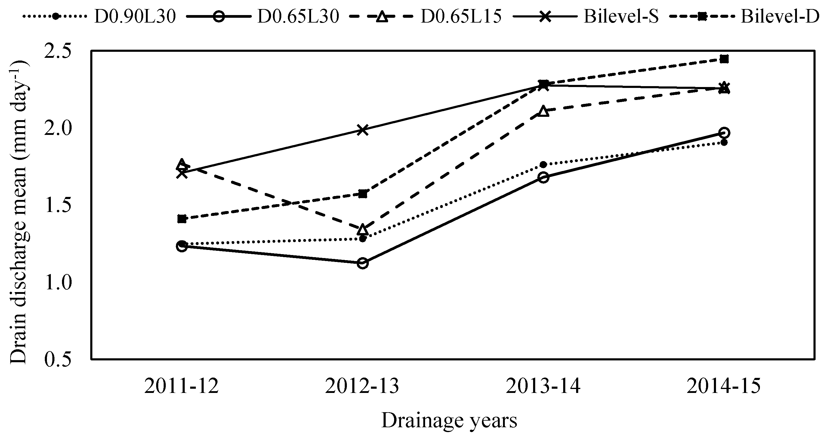
Mean drain discharge in each growing season in different drainage systems are shown in Figure 3. After this, the Bi-level-D and Bi-level-S are deep and shallow drains of the Bi-level system, respectively. In the first season, minimum and maximum drain discharges were 1.23 and 1.77 mm·day−1 related to D0.65L30 and D0.65L15, respectively. By increasing the drain spacing, the rate of drain discharge decreased. The new installation of the drainage systems in the study area, heavy textured soil in the hardpan, and its low hydraulic conductivity [38] are some of the reasons for low drainage volume in the treatments with higher spacing [39]. Also, in the D0.65L15 treatment, shallower drain depth caused shorter time for water to reach drains. It was indicated that in clayey soils with dense structures in near-surface horizons, shallow subsurface drainage systems may be fundamental for rapid water flow out of the root zone [40].
Mean discharge rates of the drainage systems have increased with time. In the third and fourth seasons, the discharges were higher than that in the first and second seasons. In the fourth season, the Bi-level-D system with 1.04 mm·day−1 had the highest increase in discharge than the others. Improving the saturated hydraulic conductivity of surface layers has a direct relation with this change [27]. Also, the drain discharges of Bi-level drainage systems in most seasons were higher than that of the other systems. This shows drainage was more effective in this plot and resulted in the greatest increase in Ks and the drains’ discharge rates. Also, because of alternative depths in the Bi-level system, which were placed at two different levels, it was helpful to make more cracks. Once cracks arise in the surface soil, water from rainfall flows rapidly into the underdrains through the cracks [32]. In another result, higher discharge in Bi-level-D than Bi-level-S was observed in the present study. This demonstrated that with improved soil conditions, a deep drain discharged a greater volume of excess water than a shallow drain.
Also, due to larger area under drainage with 30 m spaced drains (D0.65L30 and D0.90L30), the discharge rates of those were less than closer-spaced drains. It was demonstrated with a two-dimensional drainage model that drain discharge is inversely and nonlinearly related to drain spacing across a range of spacings from 5 to 50 m [41]. In the second season, the discharge rate in the D0.65L15 system was lower than other seasons. This could be due to shallow depth of drain, more surface runoff, and dense soil structure.
The variation of daily drain discharge during five days after initial water table occurring (raised up to surface) in each growing season for different drainage systems are presented in Figure 4, Figure 5, Figure 6, Figure 7 and 
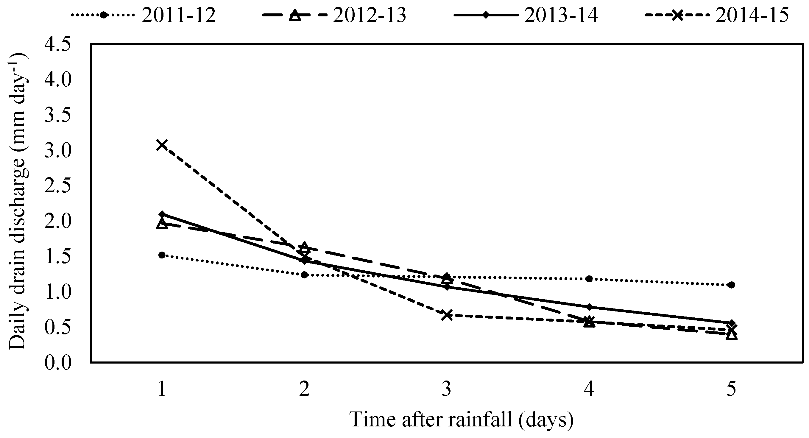
Figure 8. The drain discharges in first day for D0.90L30 were the highest in the fourth season and the lowest in the first season (Figure 4). During the first season, the drain discharge decreased gradually in later days. By the seasons, the rate of drain discharge improved and the slope of the represented line increased. This means that more excess water was drained during the first and second days after rainfall. Increase in saturated hydraulic conductivity caused an increase in drain discharge in the first and second days, that can be more effective in draining excess rainfall and protects crop from waterlogging stress.
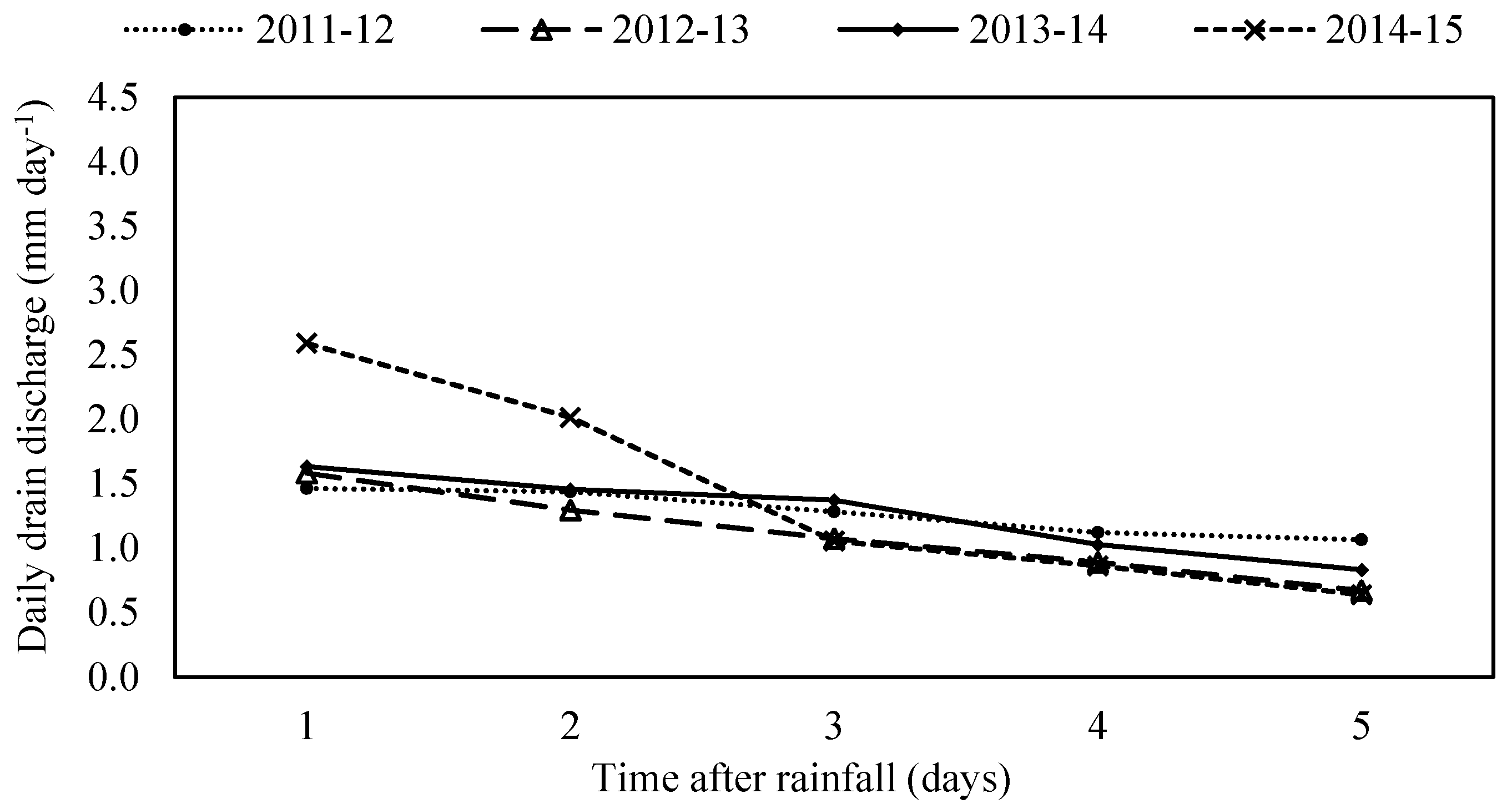
In the D0.65L30 treatment, as shown in Figure 5, the highest and lowest discharge rate in the first day were 2.59 and 1.47 mm·day−1, related to the fourth and first season, respectively. Due to shallow depth and wide spacing and small variation in saturated hydraulic conductivity (Table 6), the drain discharge rates had no major differences and varied gradually. Also, based on considerable variation in discharges from the fourth year, it can be implied that an increase in saturated hydraulic conductivity in this treatment has started after three years.
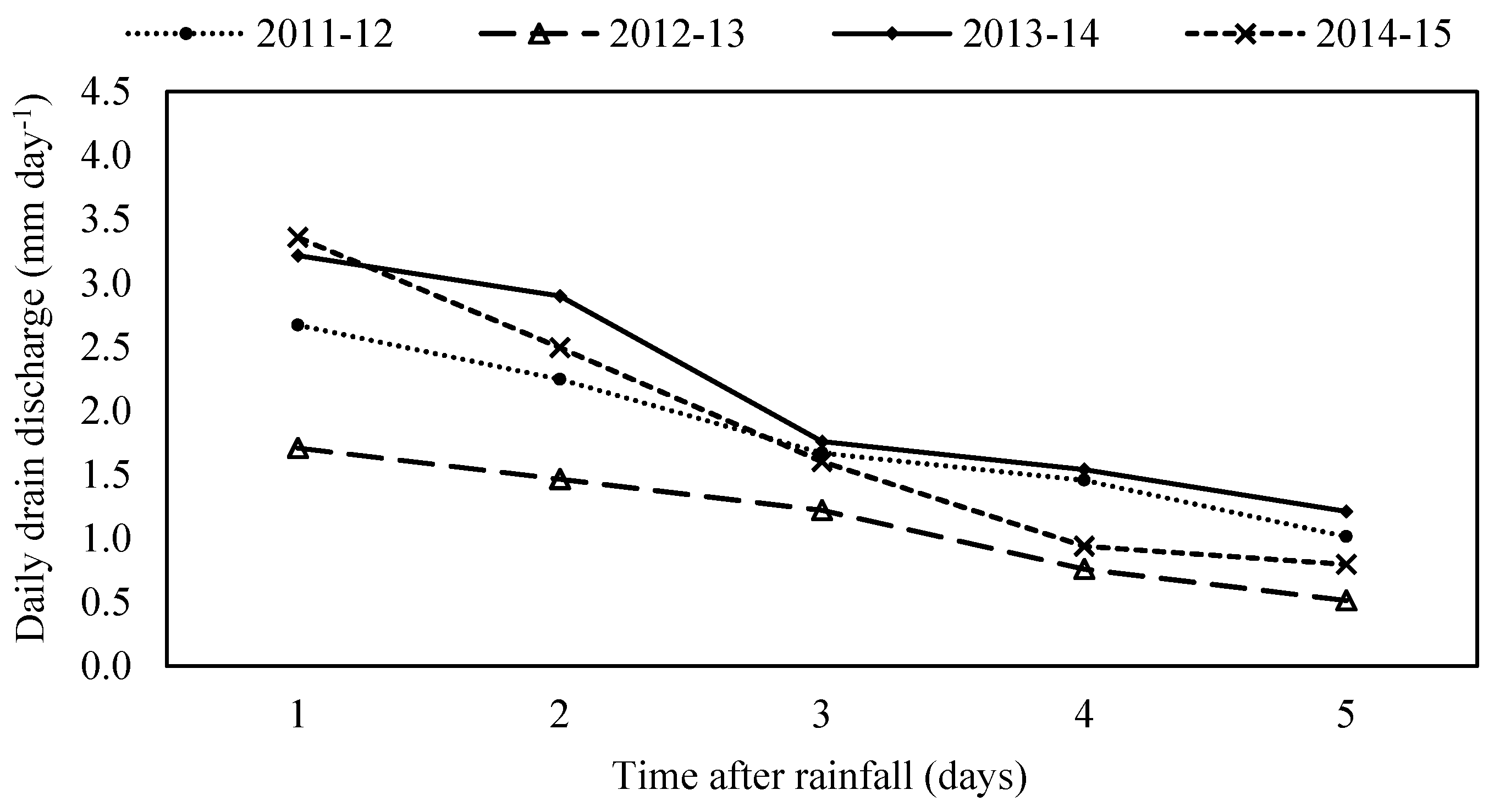
In the D0.65L15 treatment (Figure 6), the daily discharge rates decreased quickly. Due to close spacing and also shallow depth with smaller effect of hardpan layer, more excess water was discharged during the first and second days. Depth and spacing of drains as design parameters of a drainage system influence the amount of water entering drains from both saturated and unsaturated regions [39]. Also, increasing in drain discharge by the seasons was done gradually and resulted in constantly increasing saturated hydraulic conductivity.
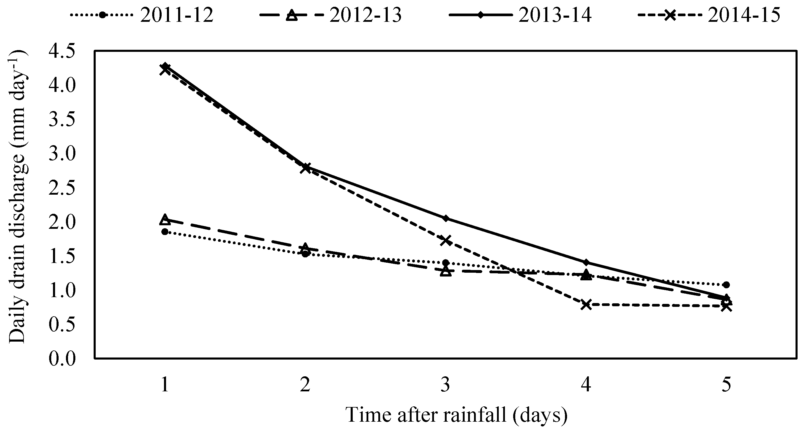
In Bi-level-S as shallow drain (Figure 7), the differences among discharges were less in comparison with Bi-level-D as deep drain (Figure 8). Furthermore, by improving the performance of drains and soil hydraulic conditions since the third and fourth seasons, both drain lines have discharged more excess water in the first day. Actually, two years after drain installation, improvement in soil condition and drain discharge was observed in this treatment.
In Table 9, the differences between drain discharges of the first and 5th days in different drainage systems along with related water tables for each year are presented. The highest value of differences was observed in the fourth season (2014–2015). The monitoring programs during the four years after the installation of the subsurface drainage systems clearly show that the subsurface drainage systems increased the drain discharge of the first day, although there were differences between the treatments. In the D0.90L30 and D0.65L15 treatments, increases in drain discharge over the years were gradual, but in the D0.65L30 and Bi-level treatments, considerable increases in drain discharge were observed from third and fourth years, respectively. It can be concluded that the differences in drain discharges are influenced by soil condition improvement. Also, in the fourth year, deep drains (D0.90L30 and Bi-level-D) had the highest difference between daily drain discharges, because they discharged most of the excess water during the first days. A study [42] found that a deep drain pipe resulted in higher tile flow. The present research has also shown that soil properties can influence tile hydrology. The plow sole layer plays a major buffering role for water flow during both dry and wet seasons [43]. However, by the time of soil structure improvement, better operation from drains can be observed.

3.3. Long-Term Effects of Subsurface Drainage Systems on Water Table Depth

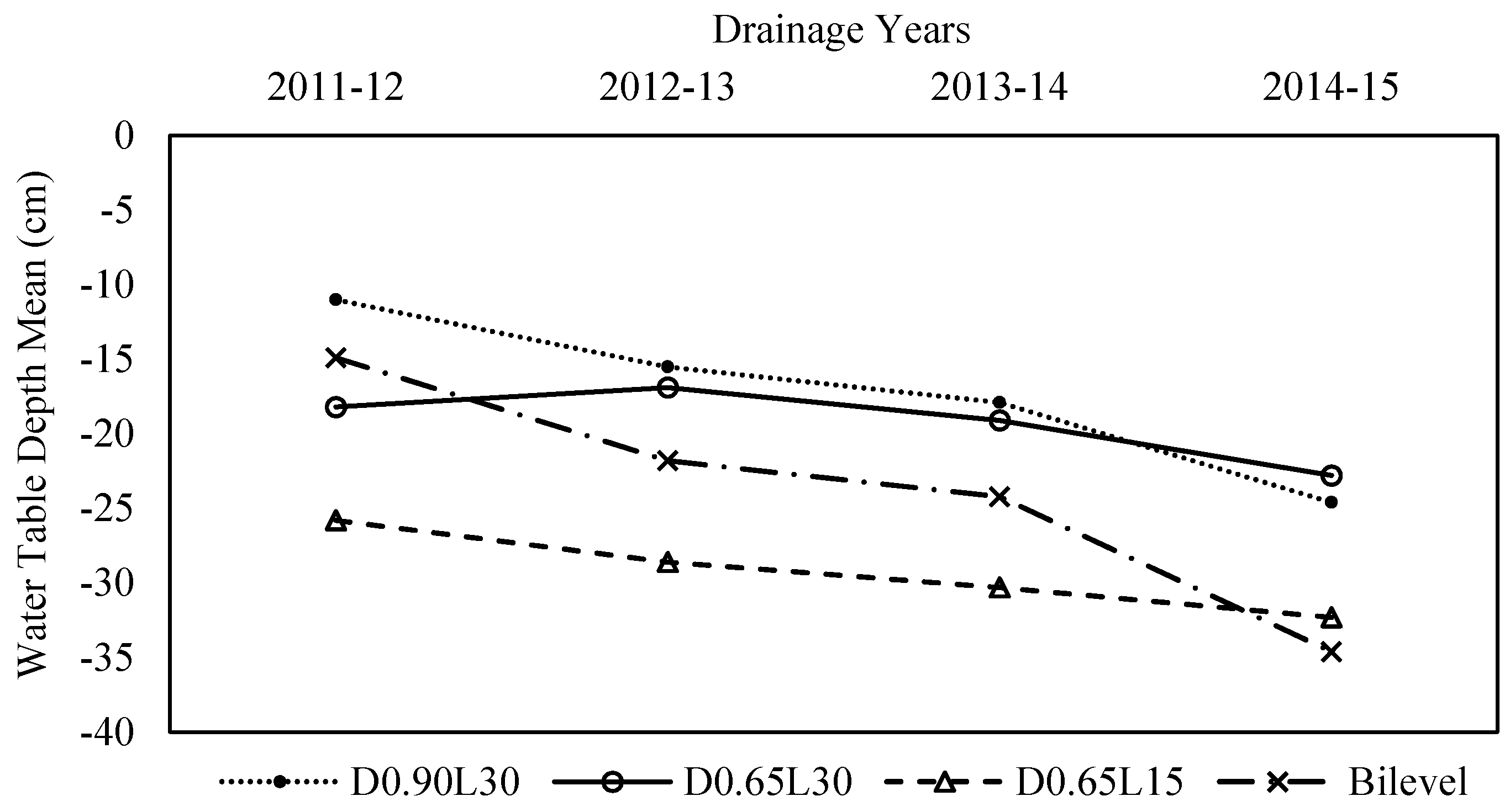
Fluctuation of the water table due to the effect of subsurface drain depth and spacing was also studied. The mean water table depth for each treatment over the seasons are presented in Figure 9. Drain systems with narrow spacing (D0.65L15) had lower water table depth than wider spacing (D0.65L30). In assessing the impacts of subsurface drainage on water table depth in northwest Minnesota, drainage systems with 12 m spacing were more effective than that with 24 m spacing [44], which is the same as the result of the present study. Moreover, due to heavy soil in paddy fields and the existence of hardpan layer [22], the performance of shallow drains in lowering the water table was better in the first season. Deeper drains do not necessarily result in a lower water table [7].
Generally, the mean water tables became deeper from year to year. However, decrease in water table depth for D0.65L30 in the second year in comparison with other years could be due to high rainfall during this season (599 mm). By improving the soil conditions for water movement and also increasing drain discharges, the performance of deep drainage systems (Bi-level and D0.90L30) improved. The highest increases in water table depth during the four seasons happened in the Bi-level drainage system with an increase of 19.7 cm. Finally, in the fourth season, deep drainage systems had better performance in draining excess water with respect to shallow drainage systems. Since the water table in the D0.90L30 treatment was deeper than in D0.65L30.
Table 10 presents the differences among the water table depths at the fourth year and also for the whole study period. The shallowest water table depth in the fourth year was related to D0.65L30. In the Bi-level system, the water table dropped more than others and it was 52% deeper than D0.65L30. The drop in water table depth of D0.90L30 was also 8% more than D0.65L30. This was because of improving soil condition and movement of water to lower layers. Moreover, during the study period, the D0.90L30 and D0.65L15 had the lowest and deepest water table depth, respectively. Heavy soil texture and low hydraulic conductivity during the first years were the reasons for low fall in water table in deep drains.

3.4. Long-Term Effects of Subsurface Drainage Systems on Canola Yield

The statistical analysis results of canola yields under subsurface drainage systems are shown in Table 11 and Table 12. Canola yields from the subsurface drainage treatments were from 450 kg·ha−1 to 3119 kg·ha−1, respectively, for the first and fourth seasons extending from 2011–2012 to 2014–2015. Due to waterlogging, it was not cultivated before drainage. In India, increase in crop yield after 2 or 3 years of drain installation were observed from 1400 to 2800 kg·ha−1 for wheat [15]. In the second season, grain yield increased in all treatments. Table 11 demonstrates that in the subsurface drainage plots, the yield gaps between the seasons were significant. The average grain yield increased from the first to second seasons and the second to fourth seasons by 152% and 12%, respectively (Table 12). In a similar study at Chashma Command Area Development Project of Pakistan during 2001–2004, quantitative comparison of pre- and post-project conditions of drainage revealed that crop yield increased for cotton (80%), sugarcane (94%), wheat (67%), and chili (147%) [45]. Increases in canola grain yield were obtained because of improvement in water table depth and drain discharge. As shown in Table 12, the water table depths in the fourth year were deeper than that in other years. Also, increase in canola yield from second year to fourth year can probably be related to fertilizer application.
Average yields obtained under subsurface drainage systems were noticeably significant when compared with each other (Table 11). In the first season, the D0.65L15 system had the highest grain yield because of better performance in discharge and falling water table (Table 12), but it was lower than the result of Cannel and Belford [46]. They harvested grain yield of oilseed rape (Brassica napus L.) as much as 3.26 t/ha in freely drainage treatment. One of the reasons for low yield is waterlogging (30 days the water table depth was less than 30 cm, as shown in Table 13) or shallow mean of water table (Table 12). In evaluations, a high reduction (14%–23%) in canola yield (rapeseed) was observed with a prolonged period of waterlogging, especially during winter [46,47]. In the second and fourth seasons, the canola under the Bi-level and D0.90L30 treatments had the highest grain yield, respectively. Also, there were significant differences between the D0.90L30 and Bi-level or D0.65L15 treatments in the fourth season. In a long-term study [48] to measure corn grain yield as affected by subsurface drain spacing, three drain spacings (5, 10, and 20 m) were compared. The results demonstrate that significant distance effects occurred more frequently for the 20 m spacing than for the 10 and 5 m spacings. Meanwhile, the yield under drainage systems with deeper depth (D0.90L30) were higher in the 2nd and 4th years as compared with the treatments with shallow drains (D0.65L30). This was because of more fall in water table levels during these seasons and also less number of days that the water table depth was less than 30 cm (Table 13).
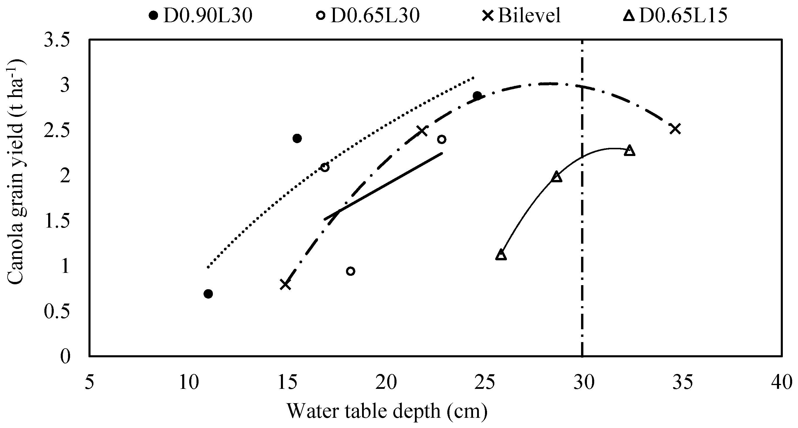
Figure 10 shows the canola grain yield in response to average of water table depth for different treatments during the study period to establish a relation between crop yield and the water table. In all treatments, the water table lowered after the introduction of subsurface drainage and crop yields increased significantly. However, the low water table may influence soil aeration, nutrient availability, and plant available moisture, but the net effect on plant growth will vary widely with crop type [49]. In this pilot, canola was harvested with yield maximum 3.1 t·ha−1, which is close to some reported values in the literature. The Canola Council of Canada [50] represented the highest canola yield of different varieties with 3.29 t·ha−1. Also, in a study in Australia, canola (Brassica napus) yields were 3–3.5 t·ha−1 and close to potential estimated [41]. So, the crop yield data analysis revealed that the objectives of drainage systems installation have been closely achieved in terms of improving the crop yields and maximum potential yield.
Basically, by lowering water table depth to optimum depth, the grain yield increases and the average of water table depth was plotted direct the average yield. Lower than optimum depth, this decreases due to much more drying and excessive drainage. By lowering water table depth to 30 cm, the grain yield of canola increased. The roots of canola are more distributed at 0–40 cm depth [51]. However, lower than 30 cm this declined, based on the results of the D0.65L15 and Bi-level treatments. Canola suffered a decrease in yield when the average water table dropped to 35 cm below the soil surface. So, it seems that average water table depth of 30 cm is optimum depth. Optimum growing conditions for canola in the area required that the water table midway between the drains would have an average depth of 30 cm. This depth is also suitable for ploughing. Therefore, the SEW30 can also be a good index for waterlogging stress. On the other hand, the D0.90L30 treatment had a direct relation between canola yield and water table depth, so this treatment needs more draining and improvement in soil condition, and can yield as much as the potential expected in future. However, in the D0.65L30 treatment, it is roughly possible to draw a direct relation between water table depth and canola yield.
Subsurface pipe drainage removes excess soil water to keep the soil moisture favorable for crop growth. From the performance point of view of drainage system operation, crop yields are generally expected to increase with the installation of subsurface drainage system [45]. Generally, canola yield as second cultivation has increased from the first to fourth seasons and along with improvement of soil aeration conditions and performance of drainage systems. The results showed direct relationship between improvement of system performance and increasing in grain yield. Moreover, improvement of soil structure and more yield after the operation will be followed by a rise in the economic level. An economic analysis showed that the cost of installing subsurface drainage systems was readily justified by annual increased rice and canola yields [9]. Also, quantifying the influence of these treatments on the salinity of drainage water indicated that by increasing drain spacing, the electrical conductivity (EC) and total salt load decreased [39]. Therefore, the D0.90L30 treatment from environmental and economical points of view have also had suitable conditions.

4. Conclusions

A field experiment was conducted in SANRU paddy fields during the rainy seasons (October to May) of 2011 to 2015 to evaluate a suitable drainage system for improving soil hydraulic properties and grain yield of lowland paddy soil. The saturated hydraulic conductivity of the soil in all treatments increased, which resulted in improved water movement in soil and drain discharge rates. Agreement between the Ks calculated with Glover–Dumm and measured in different drainage treatments indicated that the measured values were the best representation of Ks. Also, during the four growing seasons, water tables of the drainage systems lowered over time because of increasing drain discharge. On the other hand, to comprehensively describe the effect of improving water flow in such soils on crop yield, canola yield at harvest was sampled during the four years. Analysis showed that the installation of a subsurface drainage system resulted in higher crop yields as well as improving soil productivity. The D0.90L30 and Bi-level treatments had the highest canola yield in the fourth and second seasons, respectively. Optimum seasonal average depth of the water table at midway between the drains was 30 cm below the soil surface. The optimum condition with considerable increases in performance during the four years were observed more in Bi-level and D0.90L30 treatments.
Due to good conditions with deep drains and wider spacing in the improvement of paddy fields, the drains with wider spacing are recommended for these lands. On the other hand, low increase in drain depth from 0.65 m to 0.90 m, along with an increase in spacing to 30 m compared to 15 m will have less cost. From the economic point of view, material cost of denser spacing is more expensive than work cost for installation, even at a deeper level. Due to a decrease in the costs of drain installation with wider spacing, and due to the improvement of soil conditions, and the performance of these systems in two to four years, one can have cheaper drainage systems in the long run and will improve the economic situation of farmers thanks to higher yield.

Acknowledgments

The authors would like to acknowledge Sari Agricultural Sciences and Natural Resources University (SANRU) for providing land for carrying out the experiments.

Author Contributions

Abdullah Darzi-Naftchali and Mehdi Jafari-Talukolaee designed and conducted the experiments. Ali Shahnazari helped with planning and implementing the drainage systems. Mehdi Jafari-Talukolaee, Henk Ritzema and Abdullah Darzi-Naftchali wrote this paper and revised that.

Conflicts of Interest

The authors declare no conflict of interest.

References

  1. Ogino, Y.; Murashima, K. Subsurface drainage system of large size paddies for crop diversification in Japan. In Proceeding of the International Commission on Irrigation and Drainage, Fifteenth Congress, The Hague, Dutch, 8–14 August 1993.
  2. Arnold, L.A. Effect of Drain Depth on Nitrogen Losses in Drainage in Shallow Water Table Soils. M.Sc. Thesis, North Carolina State University, Raleigh, NC, USA, 2004. [Google Scholar]
  3. Jung, K.Y.; Yun, E.S.; Park, K.D.; Lee, Y.H.; Hwang, J.B.; Park, C.Y.; Ramos, E.P. Effect of subsurface drainage for multiple land use in sloping paddy fields. In Proceeding of the 19th Congress of Soil Science, Soil Solutions for a Changing World, Brisbane, Australia, 1–6 August 2010.
  4. Okamoto, M. Drainage in Japan. In proceeding of the Country report in the 7th International Drainage Workshop. Drainage for the 21st Century, Pulau Pinang, Malaysia, 17–21 November 1997.
  5. Rimidis, A.; Dierickx, W. Evaluation of Subsurface Drainage Performance in Lithuania. Agric. Water Manag. 2003, 59, 15–31. [Google Scholar] [CrossRef]
  6. RDC (Rural Development Corporation in Korea). History of agricultural land and water development projects. In Proceeding of the International Commission on Irrigation and Drainage (ICID), 24 June 1999.
  7. Abdel-Dayem, S.; Ritzema, H.P. Verification of drainage design criteria in the Nile Delta, Egypt. Irrig. Drain. Syst. 1990, 4, 117–131. [Google Scholar] [CrossRef]
  8. Azhar, A.H.; Alam, M.M.; Rafiq, M. Agricultural impact assessment of subsurface drainage projects in Pakistan–crop yield analysis. Pak. J. Water Res. 2005, 9, 1–7. [Google Scholar]
  9. Darzi-Naftchali, A.; Shahnazari, A. Influence of subsurface drainage on the productivity of poorly drained paddy fields. Eur. J. Agron. 2014, 56, 1–8. [Google Scholar] [CrossRef]
  10. El-Atfy, H.E.; Abdel-Alim, M.Q.; Ritzema, H.P. A Modified Layout of the Subsurface Drainage System for Rice Areas in the Nile Delta, Egypt. Agric. Water Manag. 1991, 19, 289–302. [Google Scholar] [CrossRef]
  11. Mathew, E.K.; Panda, R.K.; Nair, M. Influence of subsurface drainage on crop production and soil quality in a low-lying acid sulphate soil. Agric. Water Manag. 2001, 47, 191–209. [Google Scholar] [CrossRef]
  12. Satyanarayana, T.V.; Boonstra, J. Subsurface drainage pilot area experiences in three irrigated project commands of Andhra Pradesh in India. Irrig. Drain. 2007, 56, 245–252. [Google Scholar] [CrossRef]
  13. Ogino, Y.; Murashima, K. Planning and design of subsurface drainage for paddies in Japan. In proceeding of the 5th International Drainage Workshop, Lahore, Pakistan, 8–15 February 1992.
  14. Yoshiaki, K. A Long-range Agriculture and Rural Development Plan in Niigata Prefecture. Available online: https://www.jstage.jst.go.jp/article/jjsidre1965/62/6/62_6_521/_article (accessed on 2 March 2016).
  15. Ritzema, H.P.; Satyanarayana, T.V.; Raman, S.; Boonstra, J. Subsurface drainage to combat waterlogging and salinity in irrigated lands in India: Lessons learned in farmers’ fields. Agric. Water Manag. 2008, 95, 179–189. [Google Scholar] [CrossRef]
  16. Darzi-Naftchali, A.; Mirlatifi, S.M.; Shahnazari, A.; Ejlali, F.; Mahdian, M.H. Effect of subsurface drainage on water balance and water table in poorly drained paddy fields. Agric. Water Manag. 2013, 130, 61–68. [Google Scholar] [CrossRef]
  17. El-Mowelhi, N.M.; van Schilfgaarde, J. Computation of soil hydrological constants from field drainage experiments in some soils in Egypt. Trans. ASAE 1982, 25, 77–79. [Google Scholar] [CrossRef]
  18. Van Hoorn, J.W. Results of a groundwater level experimental field with arable crops on a clay soil. Neth. J. Agric. Sci. 1958, 6, 1–10. [Google Scholar]
  19. Shiratori, Y.; Watanabe, H.; Furukawa, Y.; Tsuruta, H.; Inubushi, K. Effectiveness of a subsurface drainage system in poorly drained paddy fields on reduction of methane emissions. Soil Sci. Plant Nutr. 2007, 53, 387–400. [Google Scholar] [CrossRef]
  20. Wahba, M.A.S.; Christen, E.W. Modeling subsurface drainage for salt load management in southeastern Australia. Irrig. Drain. Syst. J. 2006, 20, 267–282. [Google Scholar] [CrossRef]
  21. Christen, E.W.; Skehan, D. Design and management of subsurface horizontal drainage to reduce salt loads. J. Irrig. Drain. Eng. ASCE 2001, 127, 148–155. [Google Scholar] [CrossRef]
  22. Garg, K.K.; Das, B.S.; Safeeq, M.; Bhadoria, P.B.S. Measurement and modeling of soil water regime in a lowland paddy field showing preferential transport. Agric. Water Manag. 2009, 96, 1705–1714. [Google Scholar] [CrossRef]
  23. FAO. FAO Statistical Year Book; Food and Agriculture Organization of the United Nations: Bangkok, Thailand, 1995; p. 2014. [Google Scholar]
  24. Ogino, Y.; Ota, S. The evolution of Japan’s rice field drainage and development of technology. Irrig. Drain. 2007, 56, 69–80. [Google Scholar] [CrossRef]
  25. Verma, A.K.; Gupta, S.K.; Singh, K.K.; Chauhan, H.S. An analytical solution for design of bi-level drainage systems. Agric. Water Manag. 1998, 37, 75–92. [Google Scholar] [CrossRef]
  26. Ernst, L.F. A New Formula for the Calculation of the Permeability Factor with the Auger-Hole Method; Bouwer, H., Translator; Cornell University: Ithaca, NY, USA, 1955. [Google Scholar]
  27. Ritzema, H.P. Drainage Principles and Applications, 2nd ed.; International Institute for Land Reclamation and Improvement: the Netherlands, 1994; pp. 265–287. [Google Scholar]
  28. SAS Institute. Version 9.1.3. SAS Institute: Cary, NC, USA, 2004. [Google Scholar]
  29. Stibinger, J. Terrain Experimental Measurement of Saturated Hydraulic Conductivity on Paddy Fields in Taoyuan (Taiwan) During the Cycle of Flooded Period. Agric. Trop. Subtrop. 2009, 42, 82–89. [Google Scholar]
  30. Nguyen, D.B. Irrigation of Paddy Fields in Mekong Delta; Materials, reports and documents of Department of Water Resources; Hanoi Agriculture University: Hanoi, Vietnam, 2007. [Google Scholar]
  31. Rycroft, D.W.; Amer, M.H. Prospects for the Drainage of the Clay Soils; Irrigation and Drainage paper 51; FAO: Rome, Italy, 1995; p. 136. [Google Scholar]
  32. Tabuchi, T. Improvement of paddy field drainage for mechanization. Paddy Water Environ. 2004, 2, 5–10. [Google Scholar] [CrossRef]
  33. Smedema, L.K.; Rycroft, D.W. Land drainage: Planning and design of Agricultural Drainage Systems; Batsford: London, UK, 1983; p. 376. [Google Scholar]
  34. Ramana Rao, K.V.; Bhattacharya, A.K. Salinity distribution in paddy root zone under subsurface drainage. Agric. Water Manag. 2001, 48, 169–178. [Google Scholar] [CrossRef]
  35. Darzi-Naftchali, A.; Mirlatifi, S.M.; Asgari, A. Comparison of steady- and unsteady-state drainage equations for determination of subsurface drain spacing in paddy fields: A case study in Northern Iran. Paddy Water Environ. 2014, 12, 103–111. [Google Scholar] [CrossRef]
  36. Raju, M.M.; Kumar, A.; Bisht, D.; Kumar, Y.; Sarkar, A. Representative Hydraulic Conductivity and its Effect of Variability in the Design of Drainage System. Open Access Sci. Rep. 2012, 1, 1–7. [Google Scholar]
  37. Kumar, R.; Bhakar, S.R.; Singh, P.K. Evaluation of hydraulics characteristics and management strategies of subsurface drainage system in Indira Gandhi Canal Command. Agric. Eng. Int. CIGR J. 2013, 15, 1–9. [Google Scholar]
  38. Chen, S.K.; Liu, C.W. Analysis of water movement in paddy rice fields (I) experimental studies. J. Hydrol. 2002, 260, 206–215. [Google Scholar] [CrossRef]
  39. Jafari-Talukolaee, M.; Shahnazari, A.; Ahmadi, M.Z.; Darzi-Naftchali, A. Drain discharge and salt load in response to subsurface drain depth and spacing in paddy fields. J. Irrig. Drain. Eng. ASCE 2015, 141, 171–176. [Google Scholar] [CrossRef]
  40. Turtola, E.; Paajanen, A. Influence of improved subsurface drainage on phosphorus losses and nitrogen leaching from a heavy clay soil. Agric. Water Manag. 1995, 28, 295–310. [Google Scholar] [CrossRef]
  41. Wiskow, E.; van der Ploeg, R. Calculation of drain spacings for optimal rainstorm flood control. J. Hydrol. 2003, 272, 163–174. [Google Scholar] [CrossRef]
  42. Sands, G.R.; Song, I.; Busman, L.M.; Hansen, B. The effects of subsurface drainage depth and intensity on nitrate load in a cold climate. Trans. ASABE. 2008, 51, 937–946. [Google Scholar] [CrossRef]
  43. Li, Y.; Simunek, J.; Jing, L.; Zhang, Z.H.; Ni, L. Evaluation of water movement and water losses in a direct-seeded-rice field experiment using Hydrus-1D. Agric. Water Manag. 2014, 142, 38–46. [Google Scholar] [CrossRef]
  44. Jin, C.X.; Sands, G.R.; Hansen, B.; Wiersma, J.; Kandel, H.; Fore, Z. Assessing the impacts of subsurface drainage in northwest Minnesota. In Proceeding of the ASABE Annual Internation Meeting, Las Vegas, NV, USA, 27–30 July 2003; pp. 27–30.
  45. Azhar, A.H.; Latif, M. Subsurface Drainage Impact Assessment on Crop Yield. J. Anim. Plant Sci. 2011, 21, 215–219. [Google Scholar]
  46. Cannel, R.Q.; Belford, R.K. Effect of waterlogging at different stages of development on the growth and yield of winter oilseed rape (Brassica napus L.). J. Sci. Food. Agric. 1980, 31, 963–965. [Google Scholar] [CrossRef]
  47. Boem, G.F.H.; Lavado, R.S.; Procelli, C.A. Note on the effects of winter and spring waterlogging on growth, chemical composition and yield of rapeseed. Field Crops Res. 1996, 47, 175–179. [Google Scholar] [CrossRef]
  48. Kladivko, E.J.; Willoughby, G.L.; Santini, J.B. Corn growth and yield response to subsurface drain spacing on Clermont silt loam soil. Agron. J. 2005, 97, 1419–1428. [Google Scholar] [CrossRef]
  49. Evans, R.O.; Fausey, N.R. Effects of Inadequate Drainage on Crop Growth and Yields. In Chapter II IN ASA Drainage Monograph; American Society of Agronomy: Madison, WI, USA, 1999; pp. 13–54. [Google Scholar]
  50. Canola Council of Canada. Informed Seeding Decisions. Available online: http://www.canola-council.org (accessed on 2 March 2016).
  51. Zhang, H.; Turner, N.C.; Poole, M.L. Yield of wheat and canola in the high rainfall zone of south-western Australia in years with and without a transient perched water table. Aust. J. Agric. Res. 2004, 55, 461–470. [Google Scholar] [CrossRef]
Figure 1. Location of the study area.
Sustainability 08 00249 g001
Figure 2. Layout of the subsurface drainage systems and measuring instruments ( Sustainability 08 00249 i001 
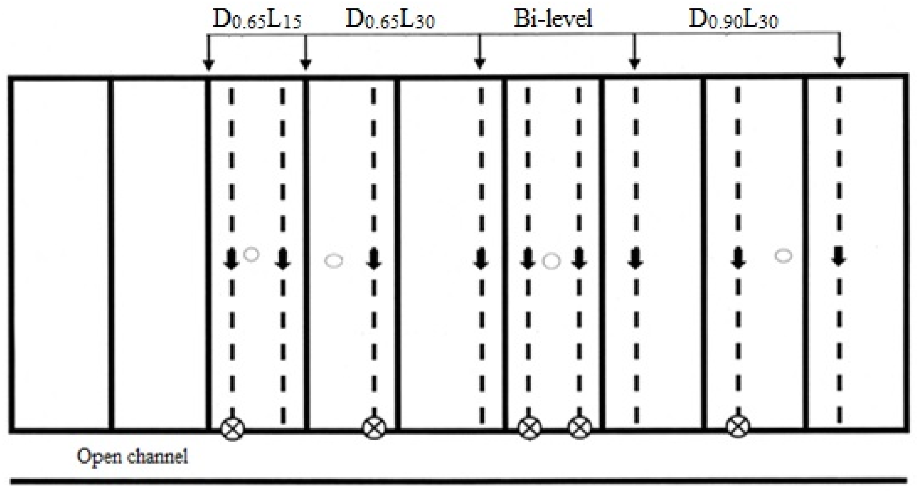
location of observation well, and Sustainability 08 00249 i002 point of drain flow measurement). D0.65L15: 0.65 m depth and 15 m spacing, D0.65L30: 0.65 m depth and 30 m spacing, Bi-level: four drains of 15 m spacing with depths of 0.90 m and 0.65 m as alternate depths, D0.90L30: 0.90 m depth and 30 m spacing.
Sustainability 08 00249 g002
Figure 3. Mean values of drain discharge for each growing season in different drainage treatments.
Sustainability 08 00249 g003
Figure 4. Daily drain discharge in D0.90L30 drainage treatment for four growing seasons.
Sustainability 08 00249 g004
Figure 5. Daily drain discharge in D0.65L30 drainage treatment for four growing seasons.
Sustainability 08 00249 g005
Figure 6. Daily drain discharge in D0.65L15 drainage treatment for four growing seasons.
Sustainability 08 00249 g006
Figure 7. Daily drain discharge in Bi-level-S drainage treatment for four growing seasons.
Sustainability 08 00249 g007
Figure 8. Daily drain discharge in Bi-level-D drainage treatment for four growing seasons.
Sustainability 08 00249 g008
Figure 9. Water table depth means in different drainage treatments for four seasons.
Sustainability 08 00249 g009
Figure 10. Canola grain yield in response to average water table depth during growing season.
Sustainability 08 00249 g010
Table 1. Monthly rainfall during the study period in the experimental site (mm).
Crop SeasonMonth2011–20122012–20132013–20142014–2015
CanolaOctober122.963.6140.083.7
November97.9111.098.876.0
December50.3173.0122.036.5
January95.464.621.531.2
February133.064.88.446.9
March82.666.472.684.9
April4.733.77.330.0
May2.822.01.210.7
Total589.6599.1471.8399.9
Table 2. Textural class of the soil of the experimental site.
Soil Depth (cm)Clay (%)Silt (%)Sand (%)Soil Texture
0–3048457Silty clay
30–6055423Silty clay
60–9047458Silty clay
90–12043516Silty clay
120–15052426Silty clay
150–20058366Clay
200–30061345Clay
Table 3. Summary of agricultural activities and fertilization during the study period.
Canola Growing SeasonTime of CultivationTime of FertilizationFertilization (kg ha−1)Time of Harvest
First28 November 20117 and 28 March 2012705 May 2012
Second4 October 20127 March 20133515 May 2013
Third----
Fourth10 October 201430 October 2014 and 14 February 20157010 May 2015
Table 4. The average Ks·(m·day−1) in different soil layers before drain installation and the differences among them.
Soil Layer (cm)Avg*St DevΔKs (%)
30–6060–9090–120120–150
0–300.273 a0.0152343270134
30–600.081 e0.005 1539642
60–900.206 b0.011 2977
90–1200.160 c0.004 37
120–1500.116 d0.010
* Means followed by the same letter in the column are not significantly different at p < 0.05 by t-test.
Table 5. Comparison between Ks means (m·day−1) of two times in different soil layers.
Soil Layer (cm)Before InstallationFour Years after InstallationΔKs (%)Significant at 0.05 Level
AvgSt DevAvgSt Dev
0–300.2730.0150.9320.167241Yes
30–600.0810.0050.1050.00529Yes
60–900.2060.0110.2530.03223Yes
90–1200.1600.0040.1600.0050No
120–1500.1160.0100.1190.0103No
Table 6. The Ks before and four years after drain installation for different drainage systems (m·day−1).
Soil Layer (cm)D0.90L30D0.65L30D0.65L15Bi-level
BeforeAfterΔKs (%)BeforeAfterΔKs (%)BeforeAfterΔKs (%)BeforeAfterΔKs (%)
0–300.2560.8002120.2870.7801720.2851.1102890.2641.040293
30–600.0810.110360.0830.100200.0870.100150.0750.11047
60–900.2070.290400.2050.22070.2210.23460.1930.27040
90–1200.1630.160-20.1580.157−10.1650.16820.1560.1571
120–1500.1090.120100.1310.13210.1110.109-20.1150.1172
Table 7. Calculated Ks (m·day−1) by Glover–Dumm equation. (ht (m) is water table height and qt (m·day−1) is corresponding drain discharge).
DateD0.90L30D0.65L30D0.65L15
htqtKshtqtKshtqtKs
05 November 20140.130.130.150.370.380.140.260.990.14
30 November 20140.630.650.160.531.480.360.404.320.41
02 December 20140.560.290.080.350.650.240.261.800.26
03 December 20140.793.070.590.592.590.570.464.300.36
04 December 20140.741.500.310.512.020.520.342.880.33
06 December 20140.510.570.170.390.860.290.281.630.22
13 February 20150.781.340.260.200.240.160.160.670.16
22 February 20150.440.460.160.360.640.230.360.790.08
04 March 20150.660.800.180.421.060.330.221.150.20
13 March 20150.750.770.150.591.440.320.351.280.14
Average0.600.960.220.431.140.320.312.000.23
Table 8. The average Ks values calculated by Glover–Dumm equation and measured data (m·day−1).
TreatmentsGlover–DummMeasuredΔ (%)Significant at 0.05 Level
D0.90L300.220.296−25.7No
D0.65L300.320.27815.0No
D0.65L150.230.340−32.4No
Table 9. The differences between drain discharges (mm·day−1) and water tables (cm) of the 1st and 5th days in each drainage treatment.
YearD0.90L30D0.65L30D0.65L15Bi-Level-SBi-Level-DBi-Level
ΔqΔhΔqΔhΔqΔhΔqΔqΔh
2011–20120.4270.408.51.6612.50.370.8711
2012–20131.57120.9110.51.19151.451.1713
2013–20141.54120.80122.00173.003.3914
2014–20152.61171.95152.56222.693.4619
Table 10. The water table depths in 2014–2015, four-year means and difference among the treatments (%).
Treatment2014–2015Difference with D0.65L30Four-Year MeansDifference with D0.65L30
D0.90L3024.6817.3−10
Bi-level34.65219.324
D0.65L3022.8029.30
D0.65L1532.34223.952
Table 11. Combined analysis of variance for the effect of drainage treatments on grain yield of canola.
Variation SourcesdfMean Square
Year (Y)227,447,498 *
Replication (R)/Y2441,718 ns
Treatment (T)3243,804 *
T×Y6611,595 *
Error7247,960
Cv (%) 11.62
ns indicates no significance.* Significant at the 0.05 level probability.
Table 12. Mean canola grain yield (Y) under different subsurface drainage systems in each season.
TreatmentSeasonal Yield (kg·ha−1)ΔY (%)Water Table Depth Means (cm)
2011–20122012–20132014–2015Average2011–20132011–20152011–20122012–20132014–2015
D0.90L30688 d2409 a2879 a1991 a2503181115.524.6
Bi-level795 c2493 a2519 b1935 a21321714.921.834.6
D0.65L30941 b2088 b2398 b1808 b12115518.216.922.8
D0.65L151129 a1991 b2279 b1799 b7610225.828.632.3
Average*888c2245 b2518 a 15218317.520.728.6
Means followed by the same letter in a column are not significantly different at p < 0.05 by LSD test; * Means followed by the same letter in this row are not significantly different at p < 0.05 by LSD test.
Table 13. Number of days that the water table depth was less than 30 cm and SEW30 under different drainage systems in each season.
TreatmentNumber of DaysSEW30 (cm)
D0.90L30D0.65L30D0.65L15Bi-levelD0.90L30D0.65L30D0.65L15Bi-Level
2011–20127550306720777662981392
2012–201364663961142810636351029
2014–201515221214410524252314
SEW30: sum of excess water above the 30 cm soil depth.

