
Multiscale Spatio-Temporal Dynamics of Economic Development in an Interprovincial Boundary Region: Junction Area of Tibetan Plateau, Hengduan Mountain, Yungui Plateau and Sichuan Basin, Southwestern China Case


Abstract
:1. Introduction
2. Materials and Methods
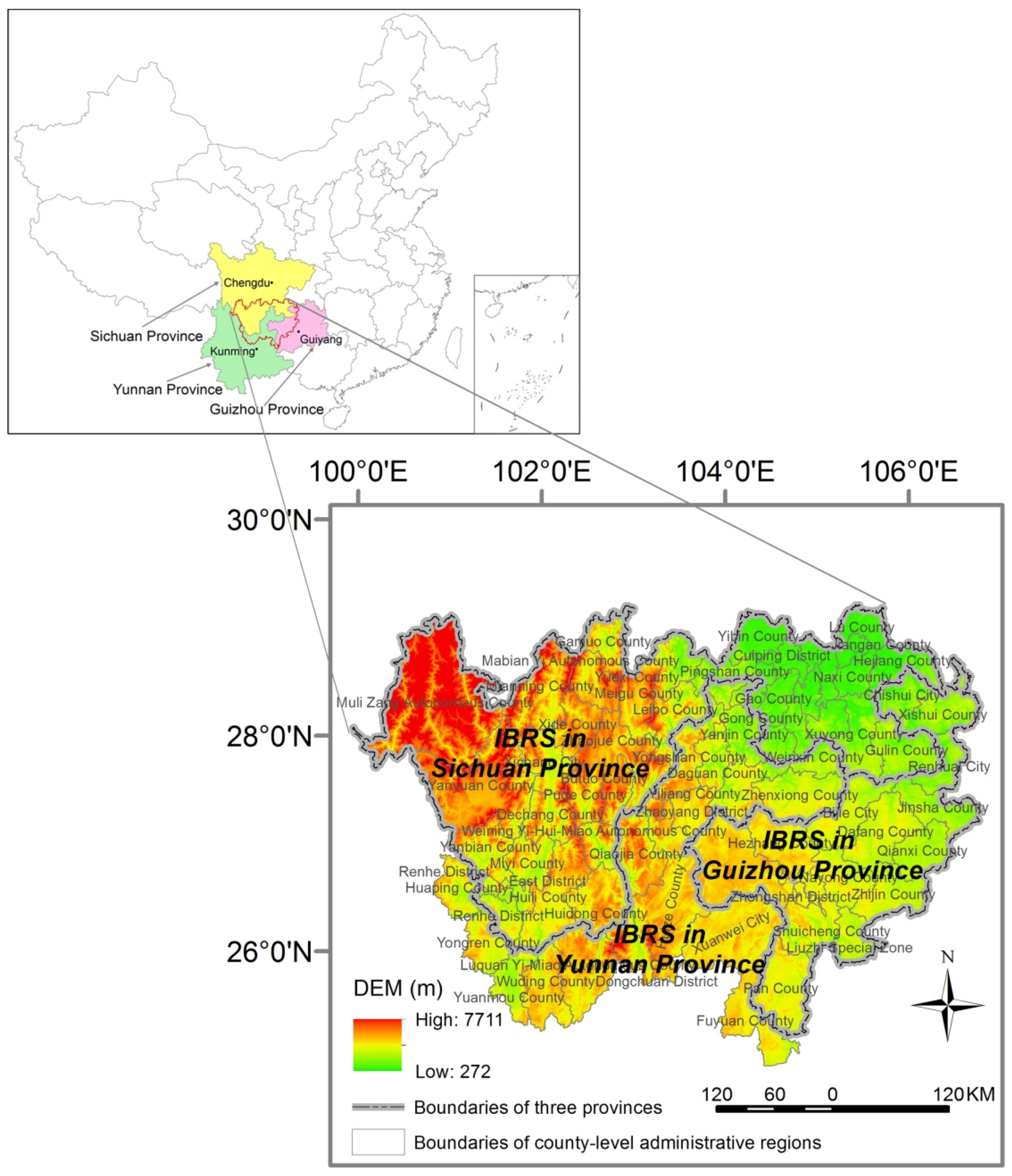
2.1. Study Area
2.2. Data
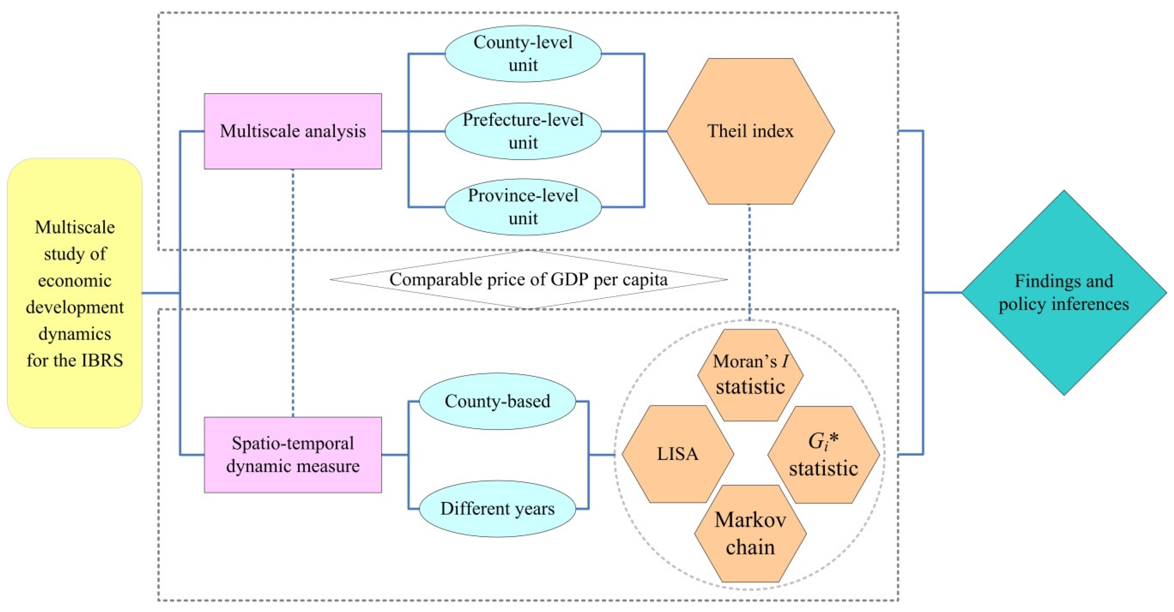
2.3. Methodology
2.3.1. Theil Index
2.3.2. Markov Chain
2.3.3. ESDA Method
3. Results and Discussion
3.1. Results
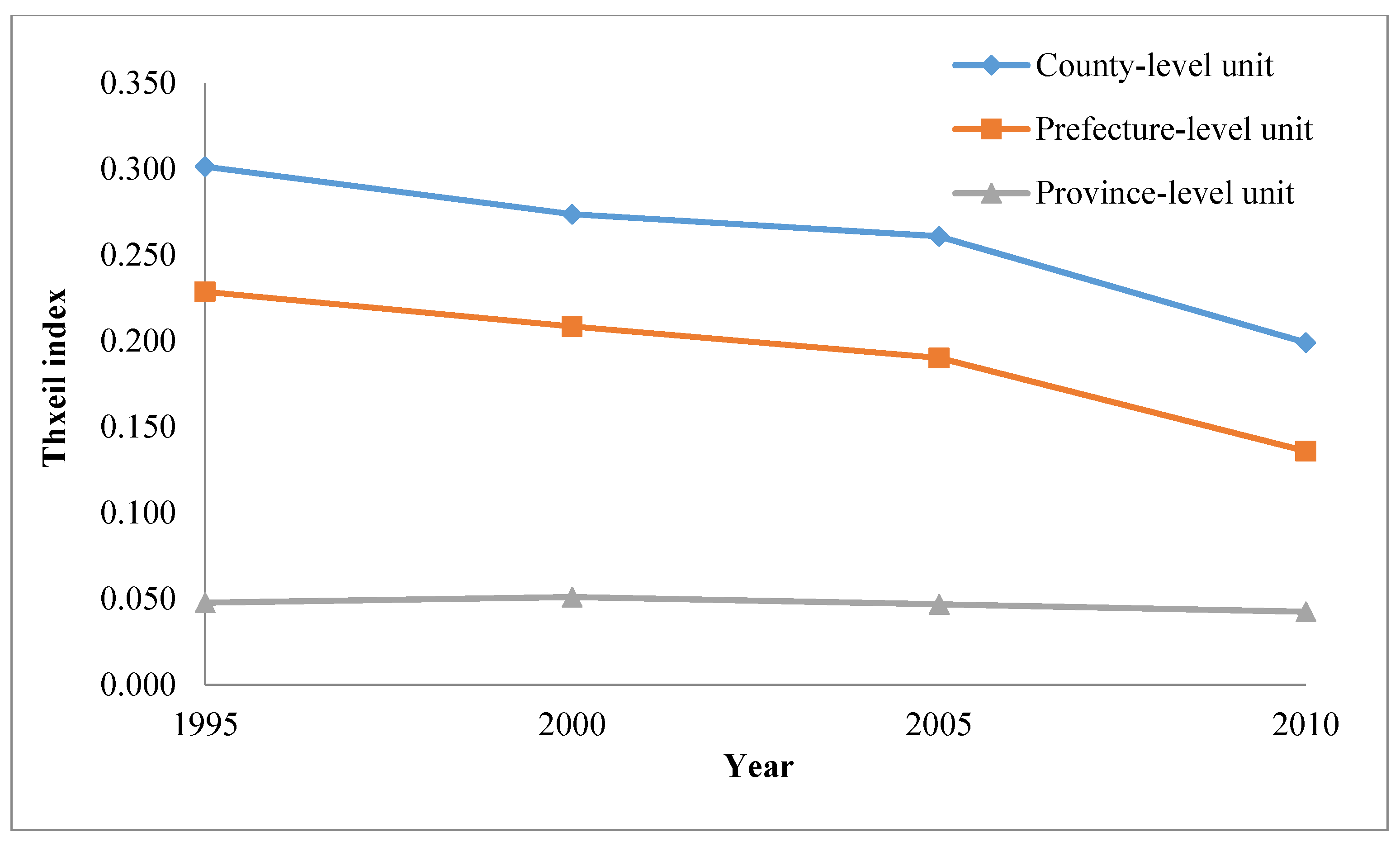
3.1.1. Scale Effect
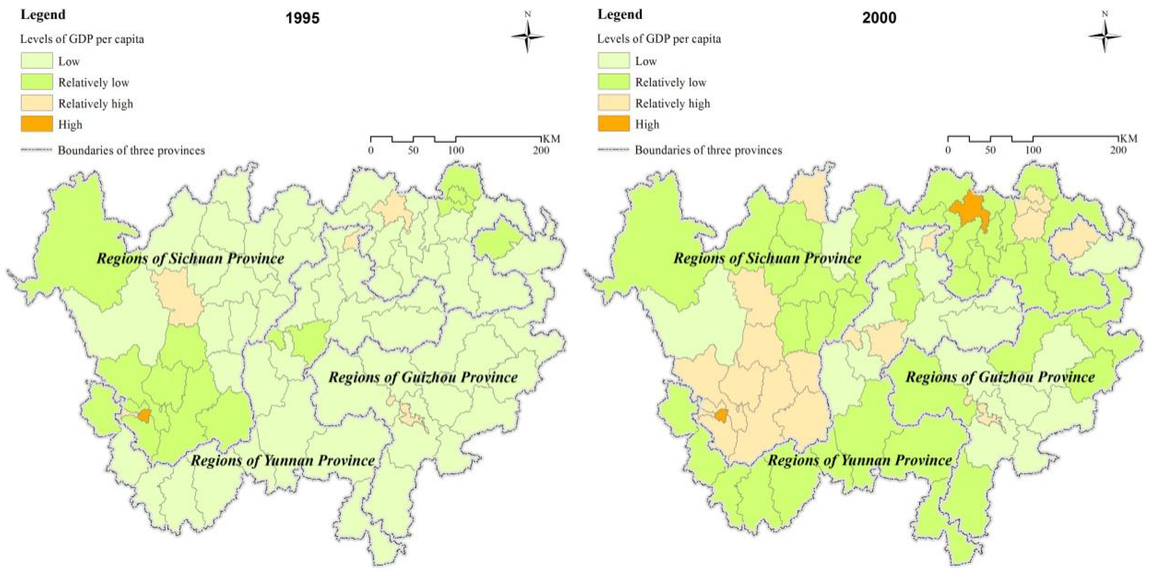
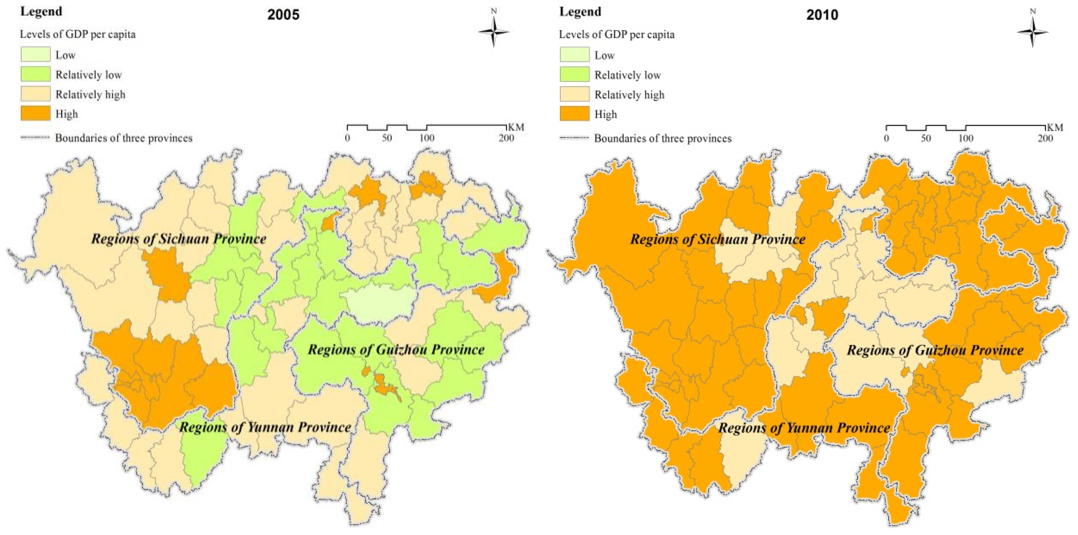
3.1.2. Spatio-Temporal Transition
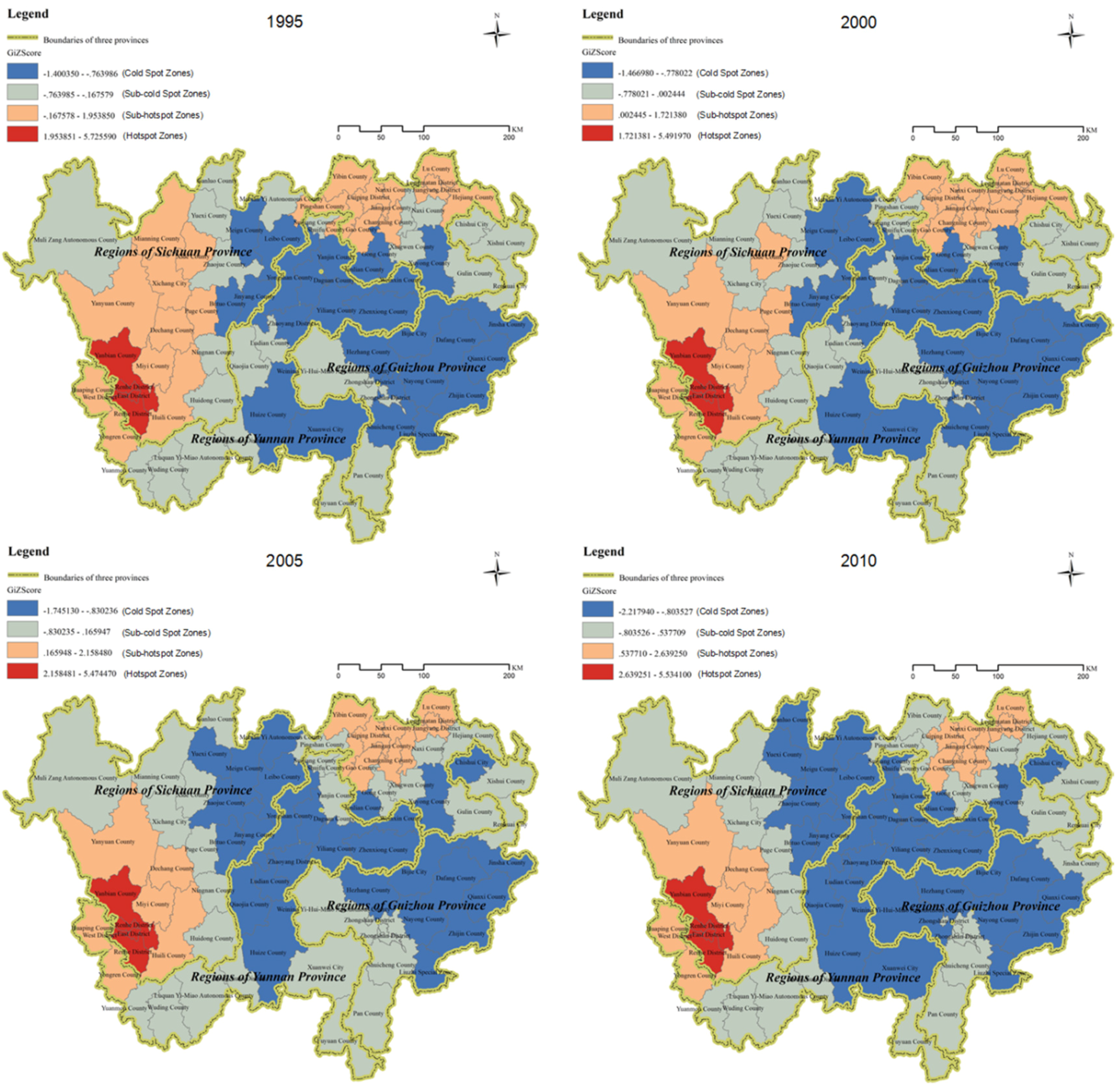
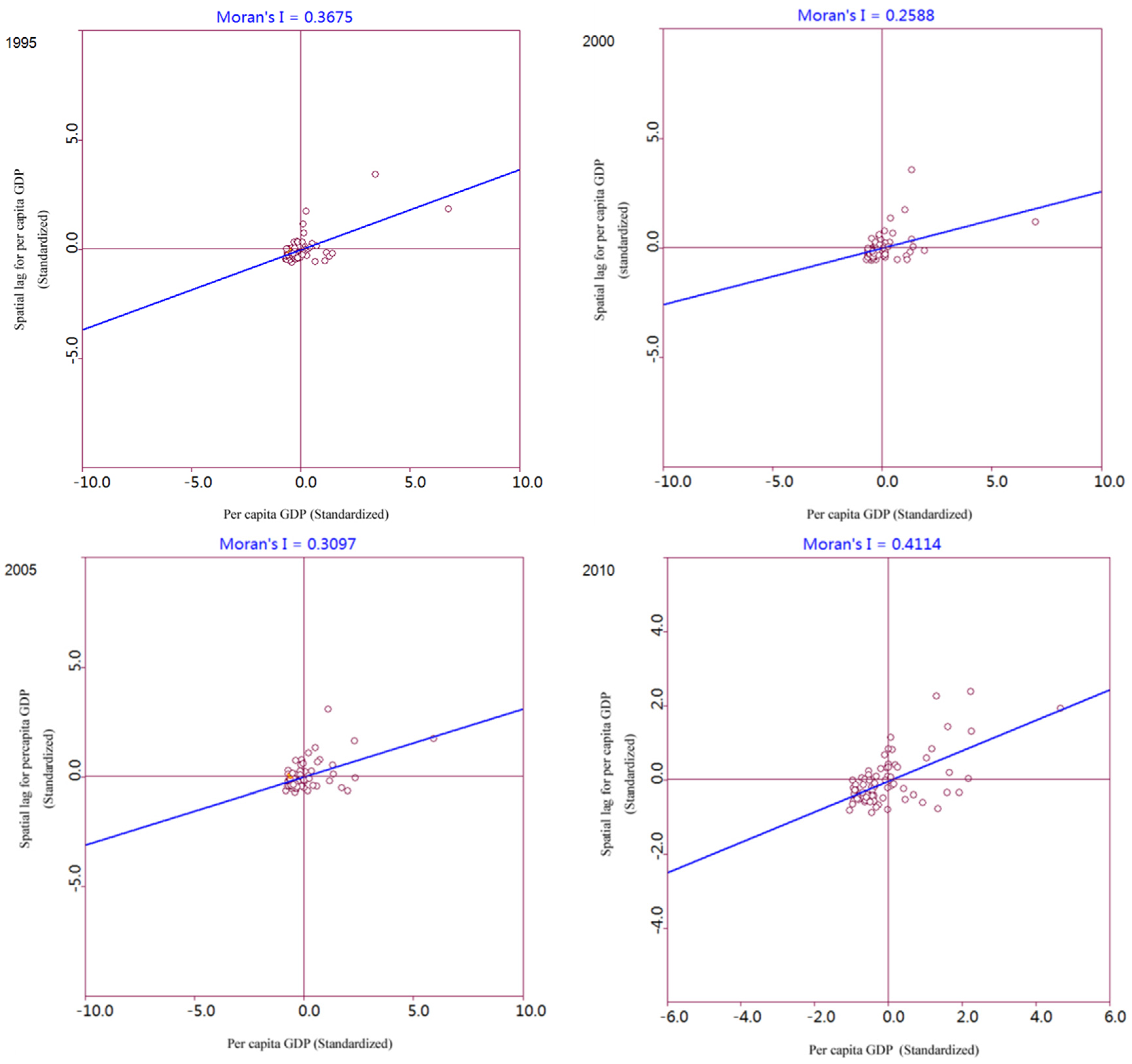
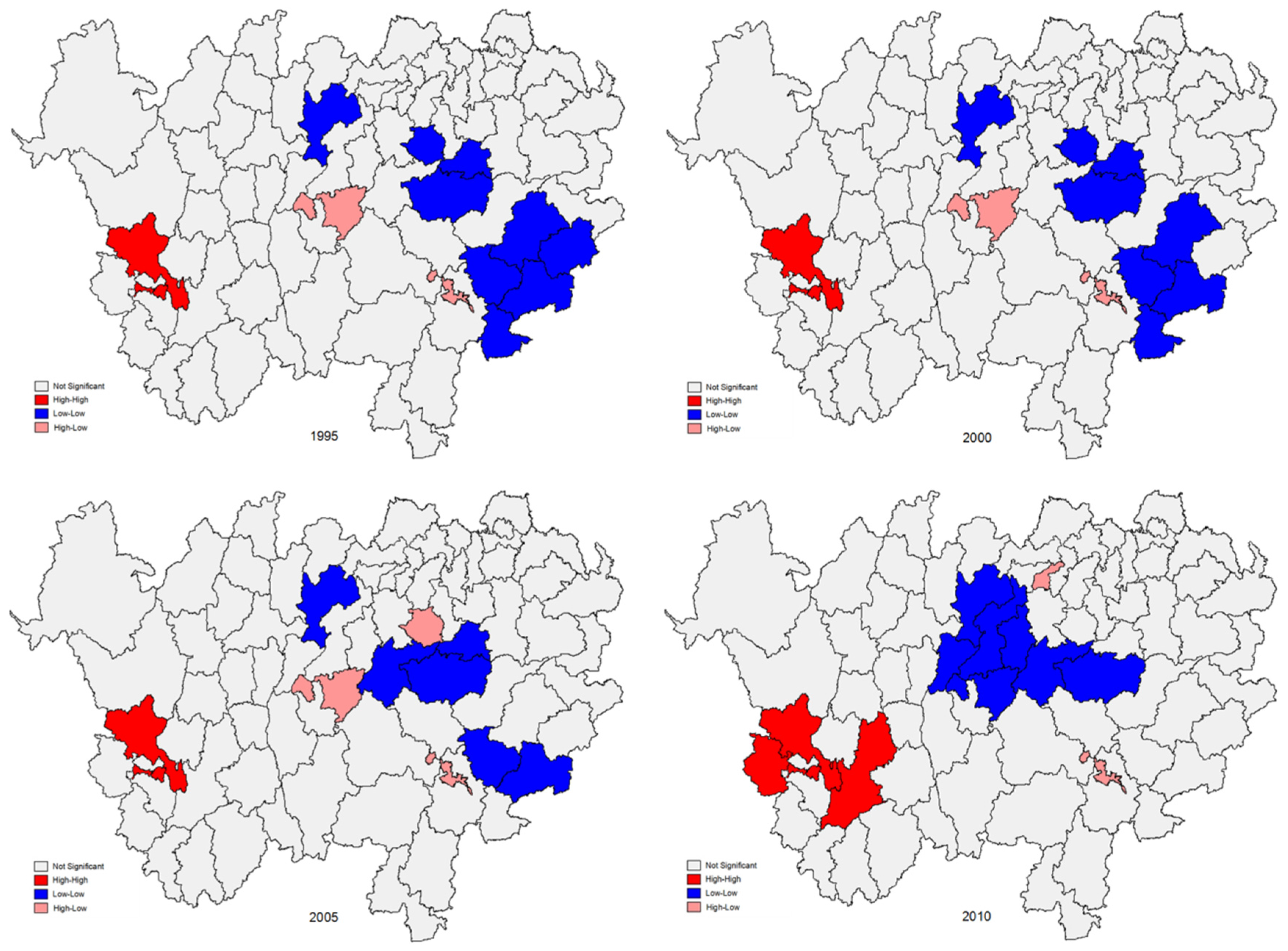
3.1.3. Spatio-Temporal Correlation
3.2. Discussion
4. Conclusions
Acknowledgments
Author Contributions
Conflicts of Interest
References
- World Bank. China Overview. 2015. Available online: www.worldbank.org/en/country/china/overview (accessed on 8 December 2015).
- Cai, F.; Wang, D.W.; Du, Y. Regional disparity and economic growth in China: The impact of labor market distortions. China Econ. Rev. 2002, 13, 197–212. [Google Scholar]
- Jones, D.C.; Li, C.; Owen, A.L. Growth and regional inequality in China during the reform era. China Econ. Rev. 2003, 14, 186–200. [Google Scholar] [CrossRef]
- Chen, M.J.; Zheng, Y.N. China’s regional disparity and its policy responses. China World Econ. 2008, 16, 16–32. [Google Scholar] [CrossRef]
- Demurger, S. Infrastructure development and economic growth: An explanation for regional disparities in China. J. Comp. Econ. 2001, 29, 95–117. [Google Scholar] [CrossRef]
- Xu, J.H.; Lu, Y.; Su, F.L.; Ai, N.S. R/S and wavelet analysis on evolutionary process of regional economic disparity in China during past 50 years. Chin. Geogr. Sci. 2004, 14, 193–201. [Google Scholar] [CrossRef]
- Lu, W.M.; Lo, S.F. A closer look at the economic-environmental disparities for regional development in China. Eur. J. Oper. Res. 2007, 183, 882–894. [Google Scholar] [CrossRef]
- Lessmann, C. Foreign direct investment and regional inequality: A panel data analysis. China Econ. Rev. 2013, 24, 129–149. [Google Scholar] [CrossRef]
- Pao, H.T.; Tsai, C.M. Modeling and forecasting the CO2 emissions, energy consumption, and economic growth in Brazil. Energy 2011, 36, 2450–2458. [Google Scholar] [CrossRef]
- Nichols, A. Income inequality, volatility, and mobility risk in China and the US. China Econ. Rev. 2010, 21, S3–S11. [Google Scholar]
- Lidia, C.; Paolo, V. The origins of the Gini index: Extracts from Variabilita e Mutabilita (1912) by Corrado Gini. J. Econ. Inequal. 2012, 10, 421–443. [Google Scholar]
- Mishra, A.; Ray, R. Prices, Inequality, and poverty: Methodology and Indian evidence. Rev. Income Wealth 2011, 57, 428–448. [Google Scholar]
- Duro, J.A.; Padilla, E. Inequality across countries in energy intensities: An analysis of the role of energy transformation and final energy consumption. Energy Econ. 2011, 33, 474–479. [Google Scholar]
- Martinez, R. Inequality and the new human development index. Appl. Econ. Lett. 2012, 19, 533–535. [Google Scholar]
- Dauth, W. Agglomeration and regional employment dynamics. Pap. Reg. Sci. 2013, 92, 419–435. [Google Scholar] [CrossRef]
- Wojcik, D. Securitization and its footprint: The rise of the US securities industry centers centers 1998–2007. J. Econ. Geogr. 2011, 11, 925–947. [Google Scholar] [CrossRef]
- Gochoco-Bautista, M.S.; Bautista, C.C.; Maligalig, D.S.; Sotocinal, N.R. Income polarization in Asia. Asian Econ. Pap. 2013, 12, 101–136. [Google Scholar]
- Wang, Y; Chen, Y.N.; Li, Z. Evolvement characteristics of population and economic gravity centers in Tarim river basin, Uygur Autonomous Region of Xinjiang, China. Chin. Geogr. Sci. 2013, 23, 765–772. [Google Scholar]
- Xie, L.N.; Zeng, S.X.; Zou, H.; Tam, V.W.Y.; Wu, Z.H. Technology transfer in clean development mechanism (CDM) projects: Lessons from China. Technol. Econ. Dev. Econ. 2013, 19, S471–S495. [Google Scholar]
- Huang, B.; Meng, L.N. Convergence of per capita carbon dioxide emissions in urban China: A spatio-temporal perspective. Appl. Geogr. 2013, 40, 21–29. [Google Scholar]
- Unwin, A.; Unwin, D.; Fischer, P. Exploratory spatial data analysis with local statistics. Stat 1998, 47, 415–421. [Google Scholar]
- Arbia, G. The role of spatial effects in the empirical analysis of regional concentration. J. Geogr. Syst. 2001, 3, 271–281. [Google Scholar] [CrossRef]
- Goodchild, M.F.; Anselin, L.; Appelbaum, R.; Harthorn, B.H. Toward spatially integrated social science. Int. Reg. Sci. Rev. 2000, 23, 139–159. [Google Scholar]
- Li, Y.R.; Wei, Y.H.D. The spatial-temporal hierarchy of regional inequality of China. Appl. Geogr. 2010, 30, 303–316. [Google Scholar]
- Porter, J.R.; Purser, C.W. Social disorganization, marriage, and reported crime: A spatial econometrics examinations of family formation and criminal offending. J. Crim. Just. 2010, 38, 942–950. [Google Scholar] [CrossRef]
- Ye, X.Y.; Wu, L. Analyzing the dynamics of homicide patterns in Chicago: ESDA and spatial panel approaches. Appl. Geogr. 2011, 31, 800–807. [Google Scholar] [CrossRef]
- Yao, J.; Murray, A.T.; Agadjanian, V.; Hayford, S.R. Geographic influences on sexual and reproductive health service utilization in rural Mozambique. Appl. Geogr. 2012, 32, 601–607. [Google Scholar] [CrossRef] [PubMed]
- Fritzell, J. Income inequality trends in the 1980s: A five country comparison. Acta Soc. 1993, 36, 47–62. [Google Scholar] [CrossRef]
- Fan, C.C. The temporal and spatial dynamics of income and population growth in Ohio, 1950–1990. Reg. Stud. 1994, 28, 241–258. [Google Scholar] [CrossRef] [PubMed]
- Fedolov, L. Regional inequality and polarization in Russia. World Dev. 2002, 30, 443–456. [Google Scholar]
- Yang, Z.S.; Cai, J.M. Progress of spatial statistics and its application in economic geography. Progr. Geogr. 2010, 29, 757–768. (In Chinese) [Google Scholar]
- Gallo, J.L.; Ertur, C. Exploratory spatial data analysis of the distribution of regional per capita GDP in Europe, 1980–1995. Pap. Reg Sci. 2003, 82, 175–201. [Google Scholar] [CrossRef]
- Ertur, C.; Koch, W. Regional disparities in the European Union and the enlargement process: An exploratory spatial data analysis, 1995–2000. Ann. Reg. Sci. 2006, 40, 723–765. [Google Scholar] [CrossRef]
- Celebioglu, F.; Dall’Erba, S. Spatial disparities across the regions of Turkey: An exploratory spatial data analysis. Ann. Reg. Sci. 2010, 45, 379–400. [Google Scholar] [CrossRef]
- Pu, Y.X.; Ge, Y.; Ma, R.H.; Huang, X.Y.; Ma, X.D. Analyzing regional economic disparities based on ESDA. Geogr. Res. 2005, 24, 965–974. (In Chinese) [Google Scholar]
- Wu, S.D.; Wang, Q. Regional economic disparities and coordination of economic development in coastal areas of southeastern China, 1995–2005. Acta Geogr. Sin. 2008, 63, 123–134. (In Chinese) [Google Scholar]
- Dong, G.P.; Guo, T.Y.; Ma, J. GIS based analysis on spatial disparity of economic growth in Beijing-Tianjin-Hebei Metropolitan Region. J. Geo-inform. Sci. 2010, 12, 797–805. (In Chinese) [Google Scholar]
- Xiong, W.; Xu, Y.L.; Wang, Y.Y. Temporal-spatial change of the county-level economic disparities in Jiangsu Province. Progr. Geogr. 2011, 30, 224–230. (In Chinese) [Google Scholar]
- Liu, Q.C.; Wang, Z. Research on geographical elements of economic difference in China. Geogr. Res. 2009, 28, 430–440. (In Chinese) [Google Scholar]
- Pan, W.Q. The economic disparity between different regions of China and its reduction: An analysis from the geographical perspective. Soc. Sci. China. 2010, 1, 72–84. (In Chinese) [Google Scholar]
- Lu, D.D.; Liu, Y.; Fan, J. The regional policy effects and regional development states in China. Acta Geogr. Sin. 1999, 54, 496–508. (In Chinese) [Google Scholar]
- Wu, D.T. A study on North-South differences in economic growth. Geogr. Res. 2001, 20, 238–246. (In Chinese) [Google Scholar]
- Guo, T.Y.; Xu, Y. The long-term trends of regional economic inequalities in China, 1952–2003. Progr. Geogr. 2005, 24, 21–30. (In Chinese) [Google Scholar]
- Ou, X.J.; Shen, Z.P.; Wang, R.C. Spatial structure evolution of regional economic growth and its inequality in China since 1978. Sci. Geogr. Sin. 2006, 26, 641–648. (In Chinese) [Google Scholar]
- Villaverde, J.; Maza, A.; Ramasamy, B. Provincial disparities in post-reform China. China World Econ. 2010, 18, 73–95. [Google Scholar] [CrossRef]
- Wang, Q.Y.; Xu, X.P. The spatial difference of regional economic develop in Jilin Province. Econ. Geogr. 2008, 28, 25–28. (In Chinese) [Google Scholar]
- Qiu, F.D.; Tong, L.J.; Zhu, C.G.; Yang, R.S. Spatio-temporal pattern and driving mechanism of economic development discrepancy in provincial border-regions: A case study of Huaihai economic zone. Geogr. Res. 2009, 28, 451–463. (In Chinese) [Google Scholar]
- Guo, R.X. The impact of spatial organizational structures on the economic development of provincial border-regions. Sci. Geogr. Sin. 1993, 13, 197–204. (In Chinese) [Google Scholar]
- Yu, F.M.; Zhang, Y.S.; Zhou, D.H.; Du, Z.C. Analyzing provincial border-regional economic disparities based on ESDA and GIS: A case study of Hohhot-Baotou-Ordos-Yulin Economic Zone. Progr. Geogr. 2012, 31, 997–1004. (In Chinese) [Google Scholar]
- Chen, P.Y.; Zhu, X.G. Regional inequalities in China at different scales. Acta Geogr. Sin. 2012, 67, 1085–1097. (In Chinese) [Google Scholar]
- Anonymous. Li Urges Building Yangtze River Economic Belt. Available online: http://www.chinadaily.com.cn/business/2014-04/29/content 17472684.htm (accessed on 17 February 2015).
- Anonymous. China: Yangtze River Economic Zone Proposal. Available online: http://www.gov.uk/government/publications/china-premier-li-proposes-gigantic-yangtze-river-economic-zone-may-2014/china-premier-li-proposes-gigantic-yangtze-river-economic-zone-may-2014 (accessed on 17 February 2015).
- Chen, Z.J. Study on integrated development strategy of the border of Sichuan, Yunnan, and Guizhou Province. Resour. Environ. Yangtza Basin 1994, 3, 193–199. (In Chinese) [Google Scholar]
- Pan, K.W.L.; Wu, N.; Pan, K.Z.; Chen, Q.H. Adiscussion on the issues of the re-construction of ecological shelter zone on the upper reaches of the Yangtze River. Acta Ecol. Sin. 2004, 24, 617–629. (In Chinese) [Google Scholar]
- Statistical Bureau of Sichuan, National Bureau of Statistics of China Survey Office in Sichuan. Sichuan Statistical Yearbook 1996; China Statistics Press: Beijing, China, 1996. (In Chinese) [Google Scholar]
- Statistical Bureau of Sichuan, National Bureau of Statistics of China Survey Office in Sichuan. Sichuan Statistical Yearbook 2001; China Statistics Press: Beijing, China, 2001. (In Chinese) [Google Scholar]
- Statistical Bureau of Sichuan, National Bureau of Statistics of China Survey Office in Sichuan. Sichuan Statistical Yearbook 2006; China Statistics Press: Beijing, China, 2006. (In Chinese) [Google Scholar]
- Statistical Bureau of Sichuan, National Bureau of Statistics of China Survey Office in Sichuan. Sichuan Statistical Yearbook 2011; China Statistics Press: Beijing, China, 2011. (In Chinese) [Google Scholar]
- Statistical Bureau of Yunnan, National Bureau of Statistics of China Survey Office in Yunnan. Yunnan Statistical Yearbook 1996; China Statistics Press: Beijing, China, 1996. (In Chinese) [Google Scholar]
- Statistical Bureau of Yunnan, National Bureau of Statistics of China Survey Office in Yunnan. Yunnan Statistical Yearbook 2001; China Statistics Press: Beijing, China, 2001. (In Chinese) [Google Scholar]
- Statistical Bureau of Yunnan, National Bureau of Statistics of China Survey Office in Yunnan. Yunnan Statistical Yearbook 2006; China Statistics Press: Beijing, China, 2006. (In Chinese) [Google Scholar]
- Statistical Bureau of Yunnan, National Bureau of Statistics of China Survey Office in Yunnan. Yunnan Statistical Yearbook 2011; China Statistics Press: Beijing, China, 2011. (In Chinese) [Google Scholar]
- Statistical Bureau of Guizhou, National Bureau of Statistics of China Survey Office in Guizhou. Guizhou Statistical Yearbook 1996; China Statistics Press: Beijing, China, 1996. (In Chinese) [Google Scholar]
- Statistical Bureau of Guizhou, National Bureau of Statistics of China Survey Office in Guizhou. Guizhou Statistical Yearbook 2001; China Statistics Press: Beijing, China, 2001. (In Chinese) [Google Scholar]
- Statistical Bureau of Guizhou, National Bureau of Statistics of China Survey Office in Guizhou. Guizhou Statistical Yearbook 2006; China Statistics Press: Beijing, China, 2006. (In Chinese) [Google Scholar]
- Statistical Bureau of Guizhou, National Bureau of Statistics of China Survey Office in Guizhou. Guizhou Statistical Yearbook 2011; China Statistics Press: Beijing, China, 2011. (In Chinese) [Google Scholar]
- Wei, Y.H.D. Multiscale and multimechanisms of regional inequality in China: Implications forregional policy. J. Contemp. China 2002, 11, 109–124. [Google Scholar] [CrossRef]
- Conceição, P.; Ferreira, P. The Young Person’s Guide to the Theil Index: Suggesting Intuitive Interpretations and Exploring Analytical Applications. 2000. Available online: http://dx.doi.org/10.2139/ssrn.228703 (accessed on 25 February 2016).
- Ye, X.Y.; Li, J.J.; Cheng, Y.Q. Multi-scale and multi-mechanism analysis of the spatial pattern and temporal change of regional economic development disparities in Zhejiang Province. Progr. Geogr. 2014, 33, 1177–1186. (In Chinese) [Google Scholar]
- Anselin, L. Interactive techniques and exploratory spatial data analysis. In Geographical Information Systems: Principles, Technical Issues, Management Issues and Applications; Longley, P.A., Goodchild, M.F., Maguire, D.J., Rhind, D.W., Eds.; Wiley: Hoboken, NJ, USA, 2005; pp. 253–266. [Google Scholar]
- Anselin, L. Spatial Econometrics. In A Companion to Theoretical Econometrics; Baltagi, B.H., Ed.; Blackwell: Oxford, UK, 2001; pp. 310–330. [Google Scholar]
- Anselin, L. Local indicators of spatial association LISA. Geogr. Anal. 1995, 27, 93–115. [Google Scholar] [CrossRef]
- Getis, A.; Ord, J.K. The analysis of spatial association by use of distance statistics. Geogr. Anal. 1992, 24, 189–206. [Google Scholar] [CrossRef]
- Dall’Erba, S. Distribution of regional income and regional funds in Europe 1989–1999: An exploratory spatial data analysis. Ann. Reg. Sci. 2005, 39, 121–148. [Google Scholar] [CrossRef] [Green Version]
- Anonymous. China, People’s Republic of: Strengthening Provincial Planning and Implementation for the Yangtze River Economic Belt. Available online: http://www.adb.org/zh/node/176121 (accessed on 17 February 2015).
- Yu, H.; Liu, S.Q.; Guo, S.L.; Zhang, H.Q. Border effect of non-equilibrium economy in contiguous areas of Sichuan, Yunnan and Guizhou Provinces. Urban. Environ. Urban. Ecol. 2011, 24, 29–32. [Google Scholar]


| Provinces | Prefectures/Cities | Counties |
|---|---|---|
| Sichuan Province | Panzhihua City (totally located in the IBRS) | East District, West District, Renhe District, Miyi County, Yanbian County (number: 5) |
| Luzhou City (totally located in the IBRS) | Jiangyang District, Naxi County, Longmatan District, Lu County, Hejiang County, Xuyong County, Gulin County (number: 7) | |
| Leshan City (partially located in the IBRS) | Mabian Yi Autonomous County (mumber: 1) | |
| Yibin City (totally located in the IBRS) | Cuiping District, Yibin County, Nanxi County, Jiangan County, Changning County, Gao County, Gong County, Junlian County, Xingwen County, Pingshan County (number: 10) | |
| Liangshan Yi Autonomous Prefecture (totally located in the IBRS) | Xichang City, Muli Zang Autonomous County, Yanyuan County, Dechang County, Huili County, Huidong County, Ningnan County, Puge County, Butuo County, Jinyang County, Zhaojue County, Xide County, Mianning County, Yuexi County, Ganluo County, Meigu County, Leibo County (number: 17) | |
| Yunan Province | Kunming City (partially located in the IBRS ) | Dongchuan District, Luquan Yi-Miao Autonomous County (number: 2) |
| Qujing City (partially located in the IBRS) | Fuyuan County, Huize County, Xuanwei City (number: 3) | |
| Zhaotong City (totally located in the IBRS) | Zhaoyang District, Ludian County, Qiaojia County, Yanjin County, Daguan County, Yongshan County, Suijiang County, Zhenxiong County, Yiliang County, Weinxin County, Shuifu County (number: 11) | |
| Lijiang City (partially located in the IBRS) | Huaping County (number: 1) | |
| Chuxiong Autonomous Prefecture (partially located in the IBRS) | Yongren County, Yuanmou County, Wuding County (number: 3) | |
| Guizhou Province | Liupanshui City (totally located in the IBRS) | Zhongshan District, Liuzhi Special Zone, Shuicheng County, Pan County (number: 4) |
| Zunyi City (partially located in the IBRS) | Xishui County, Chishui City, Renhuai City (number: 3) | |
| Bijie City (totally located in the IBRS) | Bijie City, Dafang County, Qianxi County, Jinsha County, Zhijin City, Nayong County, Weining Yi-Hui-Miao Autonomous County, Hezhang County (number: 8) |
| Time Interval | 1 | 2 | 3 | 4 | |
|---|---|---|---|---|---|
| (≤$272.09) | ($272.09–$555.93) | ($555.93–$1,299.47) | (≥$1,299.47) | ||
| 1995–2000 | 1 | 0.3036 | 0.6429 | 0.0536 | 0.0000 |
| 2 | 0.0000 | 0.2308 | 0.7692 | 0.0000 | |
| 3 | 0.0000 | 0.0000 | 0.8000 | 0.2000 | |
| 4 | 0.0000 | 0.0000 | 0.0000 | 1.0000 | |
| 2000–2005 | 1 | 0.0588 | 0.8235 | 0.1176 | 0.0000 |
| 2 | 0.0000 | 0.2564 | 0.7179 | 0.0256 | |
| 3 | 0.0000 | 0.0000 | 0.3529 | 0.6471 | |
| 4 | 0.0000 | 0.0000 | 0.0000 | 1.0000 | |
| 2005–2010 | 1 | 0.0000 | 0.0000 | 1.0000 | 0.0000 |
| 2 | 0.0000 | 0.0000 | 0.6250 | 0.3750 | |
| 3 | 0.0000 | 0.0000 | 0.0288 | 0.9722 | |
| 4 | 0.0000 | 0.0000 | 0.0000 | 1.0000 | |
| 1995–2010 | 1 | 0.0000 | 0.0000 | 0.3036 | 0.6964 |
| 2 | 0.0000 | 0.0000 | 0.0000 | 1.0000 | |
| 3 | 0.0000 | 0.0000 | 0.0000 | 1.0000 | |
| 4 | 0.0000 | 0.0000 | 0.0000 | 1.0000 |
| Year | Moran’s I | E(I) | Mean | Z(I) | p |
|---|---|---|---|---|---|
| 1995 | 0.3675 | −0.0135 | −0.0151 | 6.245902 | 0.001 |
| 2000 | 0.2588 | −0.0135 | −0.0117 | 4.176380 | 0.001 |
| 2005 | 0.3097 | −0.0135 | −0.0111 | 4.164948 | 0.001 |
| 2010 | 0.4114 | −0.0135 | −0.0138 | 5.371681 | 0.001 |
| Types | 1995 | 2000 | 2005 | 2010 | ||||
|---|---|---|---|---|---|---|---|---|
| p = Any | p < 0.05 | p = Any | p < 0.05 | p = Any | p < 0.05 | p = Any | p < 0.05 | |
| HH | 11 | 3 | 11 | 3 | 13 | 3 | 15 | 5 |
| LH | 13 | 0 | 12 | 0 | 13 | 0 | 13 | 0 |
| LL | 42 | 9 | 41 | 6 | 40 | 8 | 39 | 8 |
| HL | 9 | 4 | 11 | 5 | 9 | 4 | 8 | 3 |
© 2016 by the authors; licensee MDPI, Basel, Switzerland. This article is an open access article distributed under the terms and conditions of the Creative Commons by Attribution (CC-BY) license (http://creativecommons.org/licenses/by/4.0/).
Share and Cite
Zhang, J.; Deng, W. Multiscale Spatio-Temporal Dynamics of Economic Development in an Interprovincial Boundary Region: Junction Area of Tibetan Plateau, Hengduan Mountain, Yungui Plateau and Sichuan Basin, Southwestern China Case. Sustainability 2016, 8, 215. https://doi.org/10.3390/su8030215
Zhang J, Deng W. Multiscale Spatio-Temporal Dynamics of Economic Development in an Interprovincial Boundary Region: Junction Area of Tibetan Plateau, Hengduan Mountain, Yungui Plateau and Sichuan Basin, Southwestern China Case. Sustainability. 2016; 8(3):215. https://doi.org/10.3390/su8030215
Chicago/Turabian StyleZhang, Jifei, and Wei Deng. 2016. "Multiscale Spatio-Temporal Dynamics of Economic Development in an Interprovincial Boundary Region: Junction Area of Tibetan Plateau, Hengduan Mountain, Yungui Plateau and Sichuan Basin, Southwestern China Case" Sustainability 8, no. 3: 215. https://doi.org/10.3390/su8030215
APA StyleZhang, J., & Deng, W. (2016). Multiscale Spatio-Temporal Dynamics of Economic Development in an Interprovincial Boundary Region: Junction Area of Tibetan Plateau, Hengduan Mountain, Yungui Plateau and Sichuan Basin, Southwestern China Case. Sustainability, 8(3), 215. https://doi.org/10.3390/su8030215