
Projected Crop Production under Regional Climate Change Using Scenario Data and Modeling: Sensitivity to Chosen Sowing Date and Cultivar


Abstract
:1. Introduction
2. Methodology
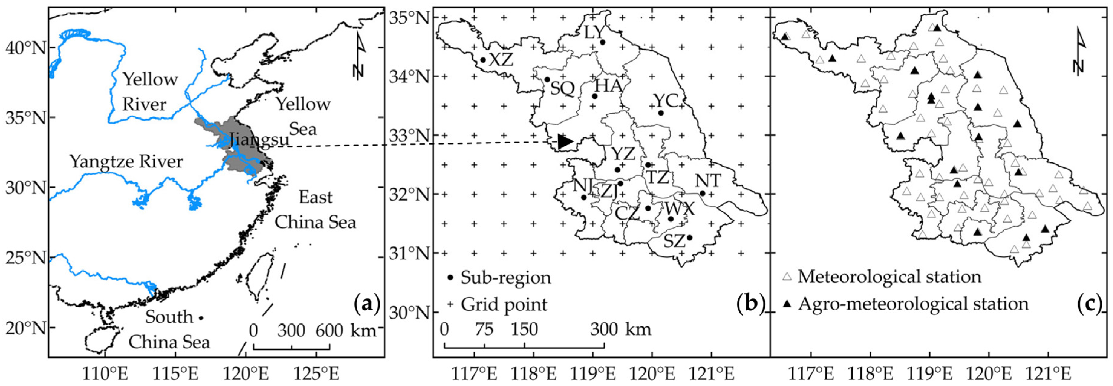
2.1. Study Region
- (i)
- The scarcity of cultivated land resources. As the economics in the province develop, the demand for non-farming construction land increases. Large areas of cultivated land have been transformed into construction land due to urbanization. The southern part of the province has a lower average amount of cultivated land per person than the northern region and a more rapid rate of decreasing farm land area [24].
- (ii)
- Observed climate change. Since 1961, the climate of this region has undergone successive cooling and warming periods. However, during recent decades, a significant warming trend has persisted. The average temperature from 2001 to 2006 increased by 1.0 °C compared with the average temperature from 1971 to 2000 [24]. However, the extent of warming varies over smaller spatial scales. The temperature is 0.9 °C greater over the Huaibei region and Jianghuai region and 1.2 °C greater over the southern Jiangsu region [24].
2.2. Data
2.3. Modeling Framework
2.3.1. The Crop Growth Model
- (i)
- First, the average sowing, emergence, anthesis and maturity dates were calculated using the observed winter wheat phenology data from the agro-meteorological stations.
- (ii)
- Second, the temperature sums were calculated using the average phenology dates and meteorological data from each agro-meteorological station.
- (iii)
- Finally, the temperature sums from sowing to emergence, from emergence to anthesis and from anthesis to maturity over the entire study region were interpolated from the results of Step (ii). For a very flat region (i.e., Jiangsu, most of which is within 50 m of sea level), it was reasonable to consider only the distances of the known points to the unknown points. In addition, because we aim to preserve the known values (i.e., observations) after spatial interpolation, a deterministic method is required. Thus, the inverse distance weights method was used.
2.3.2. Simulation Schemes
- (i)
- Running the WOFOST model under baseline and climate scenarios with average sowing dates according to the historical phenology and quantifying the changes in the winter wheat growing season, water use efficiency and water-limited yields.
- (ii)
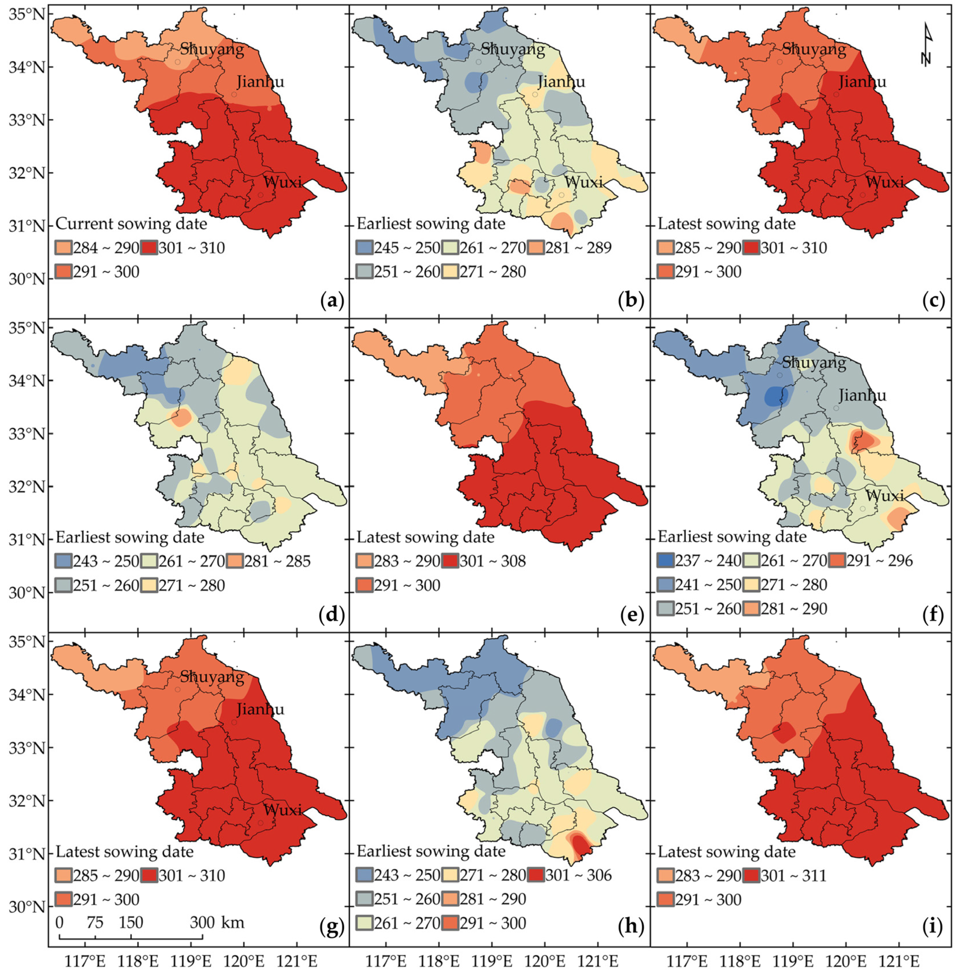
- Running the WOFOST model under climate scenarios with varying sowing dates for 2021–2050 and 2051–2080. In theory, the last date at which the daily mean temperature consistently exceeded 15 °C is treated as the latest optimal sowing date in Jiangsu. Next, the varying sowing dates for each site were established based on this date using shifts of 5 days. Sixty-day leads and 30-day lags from this date were defined as the inferior limit and superior limit of the possible sowing date interval, respectively. This varying range covered the current sowing dates (historical observations).
- (iii)
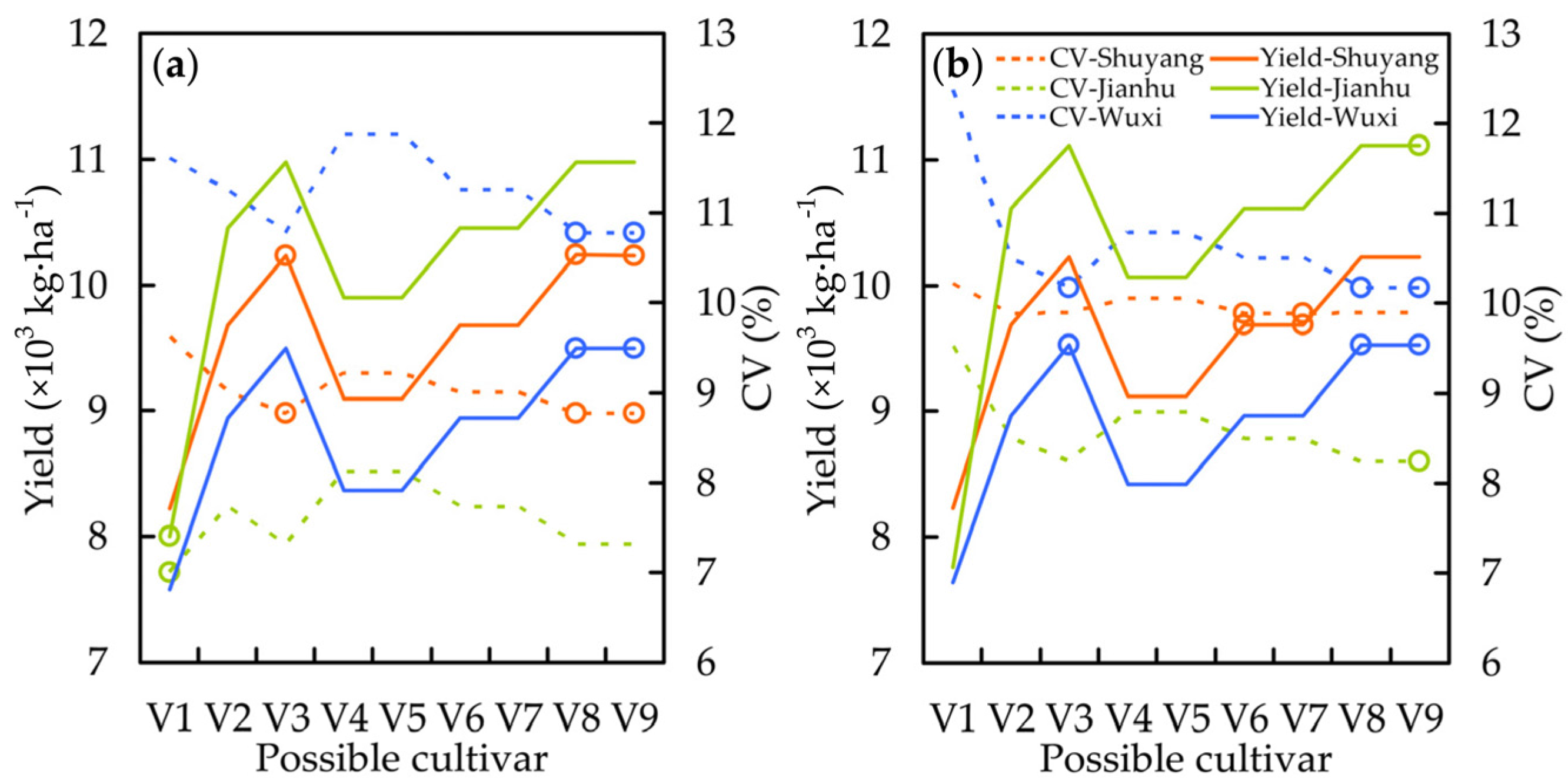
- (a)
- The minimum coefficient of variation (CV, the ratio of the standard deviation to the mean [41]) of the yield simulated using the possible sowing date (or variety) is less than or equal to the CV of the yield of the current sowing date (or variety).
- (b)
- The simulated yield is greater than or equal to the yield simulated using the current sowing date (or variety).
- (c)
- If more than one minimum is present, the CV results are equivalent, and the date (or variety) corresponding to the maximum yield is considered optimal.
3. Results
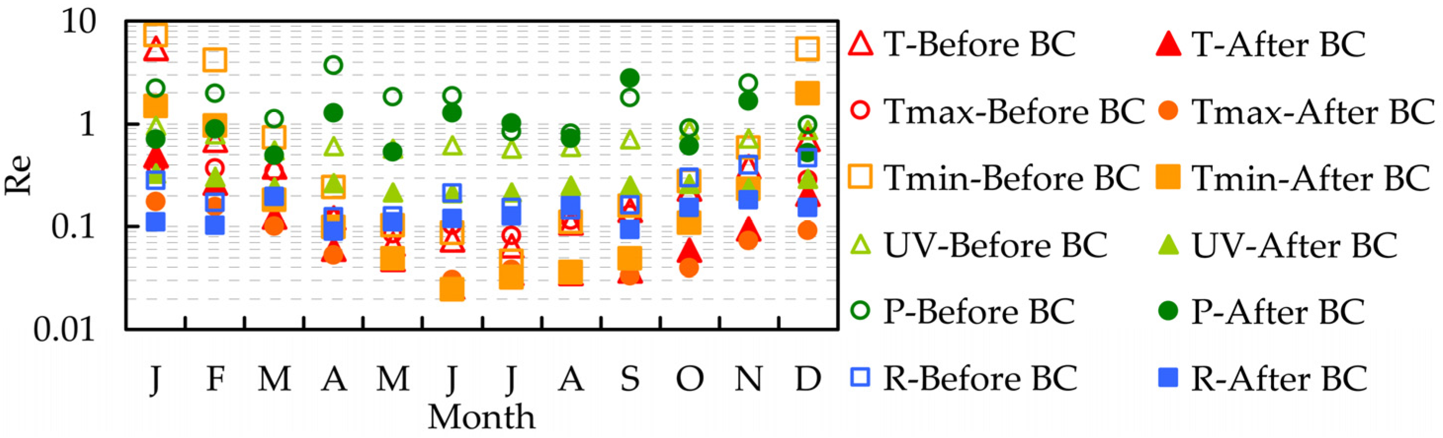
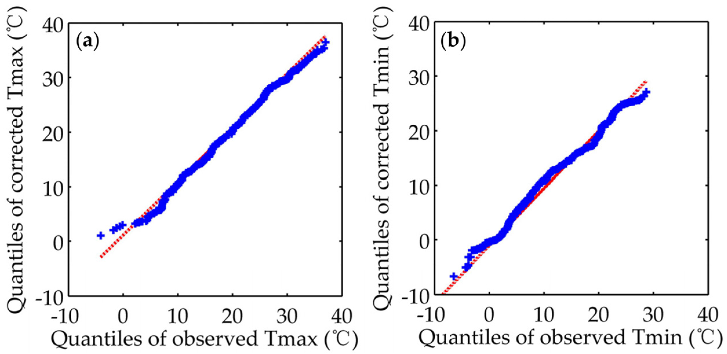
3.1. Effectiveness of the Bias Correction Method
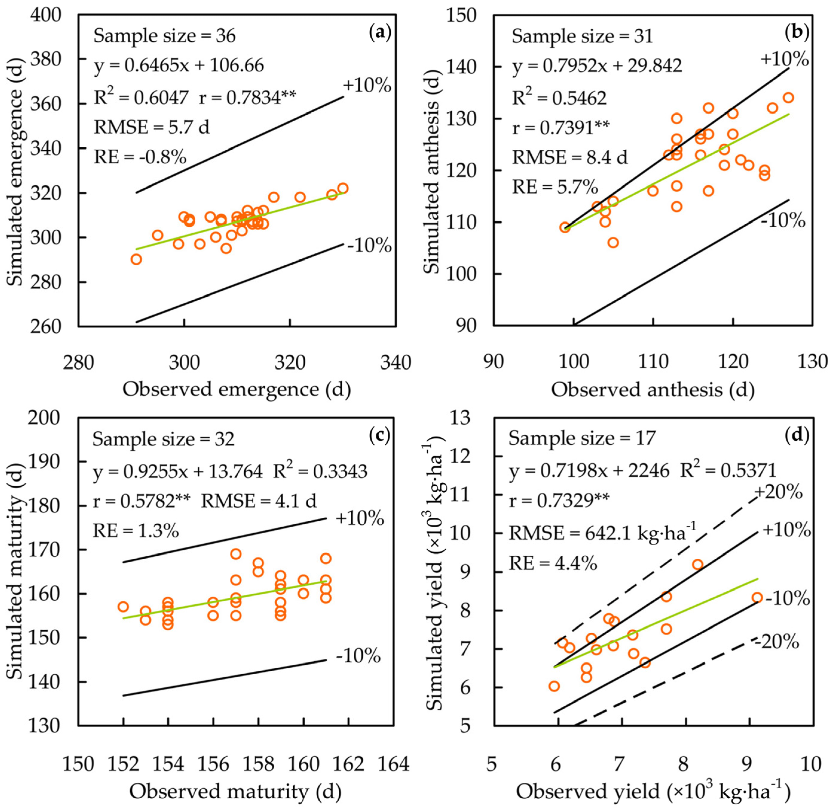
3.2. Calibration and Validation of WOFOST
- (i)
- The temperature sums from sowing to emergence, from emergence to anthesis, and from anthesis to maturity ranged from 80.0 to 140.0 °C·d, 1380.0 to 2000.0 °C·d, and 600.0 to 800.0 °C·d, respectively. Higher temperature sums from sowing to emergence and from emergence to anthesis were required by the winter wheat in northern Jiangsu than in southern Jiangsu. However, lower temperature sums from anthesis to maturity were required by winter wheat in northern Jiangsu compared with southern Jiangsu.
- (ii)
- The dominant soil groups within the province include Acrisols, Alisols, Anthrosols, Fluvisols, Gleysols, Luvisols, Planosols, Regosols, Solonchaks and Vertisols. In most areas of the province, the soil moisture contents at the wilting point, field capacity and saturation ranged from 4.7% to 33.3% cm3·cm−3, 9.7% to 44.6% cm3·cm−3 and 44.8% to 52.0% cm3·cm−3, respectively. The hydraulic conductivities of the saturated soil varied from 2.1 to 277.2 cm·d−1 and were different in the different areas of the province. The various soil groups likely account for the complex spatial patterns of these soil parameters, especially over central and northern Jiangsu.
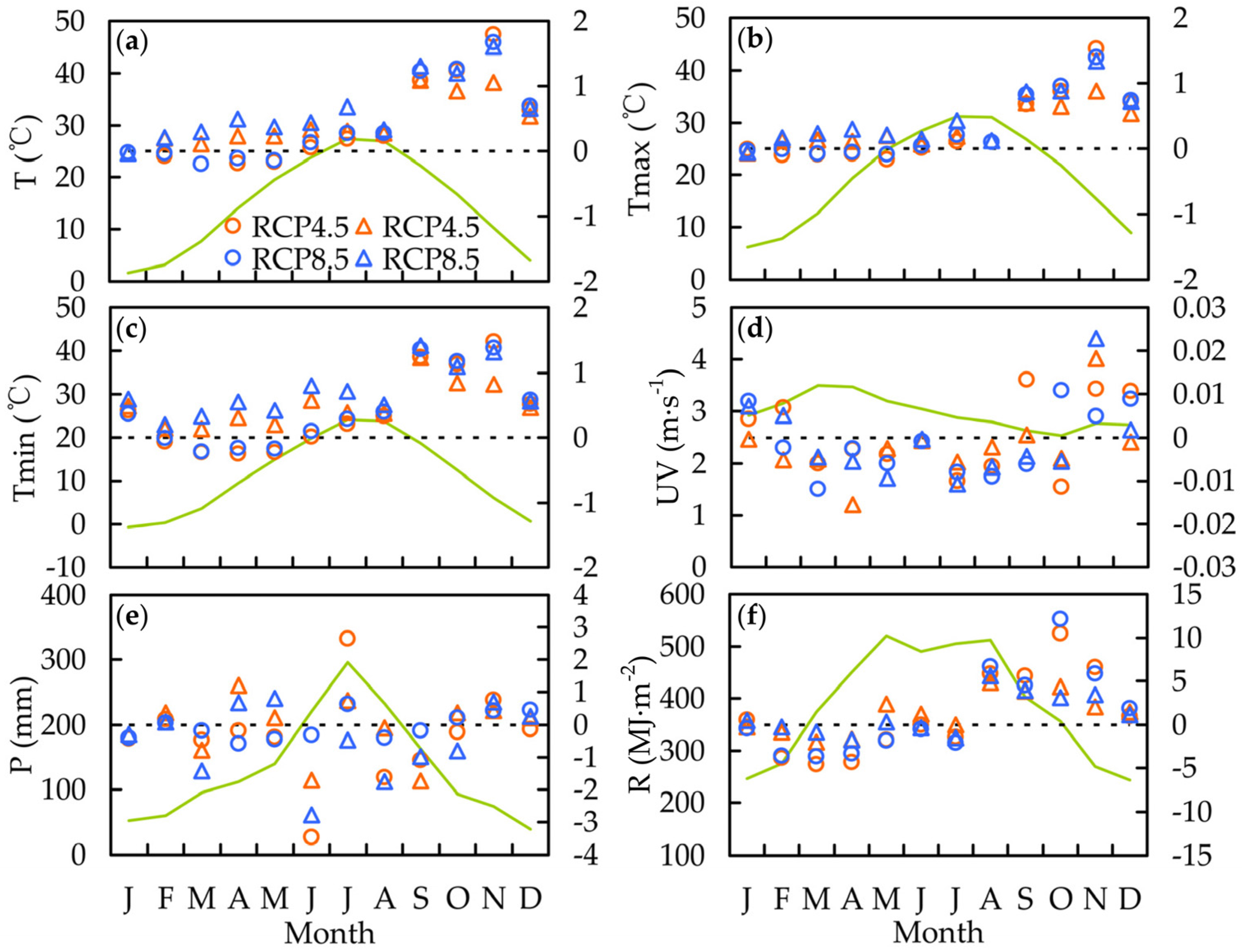
3.3. Corrected Climate Scenario Projections
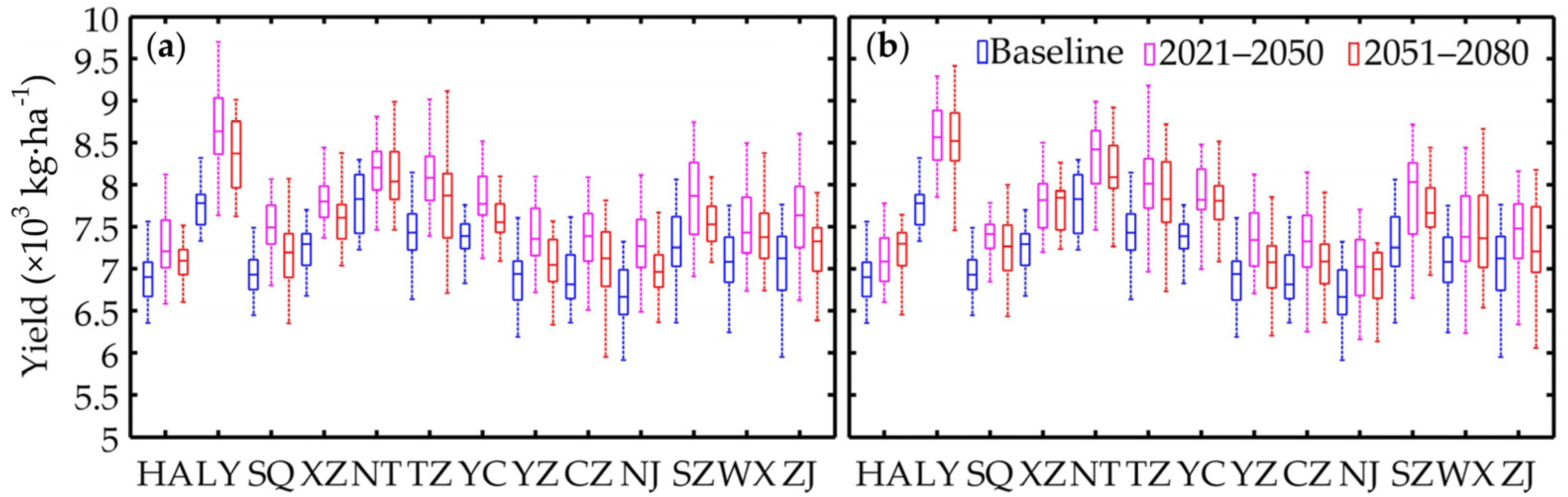
3.4. Projected Results from Using the Current Sowing Date and Cultivar
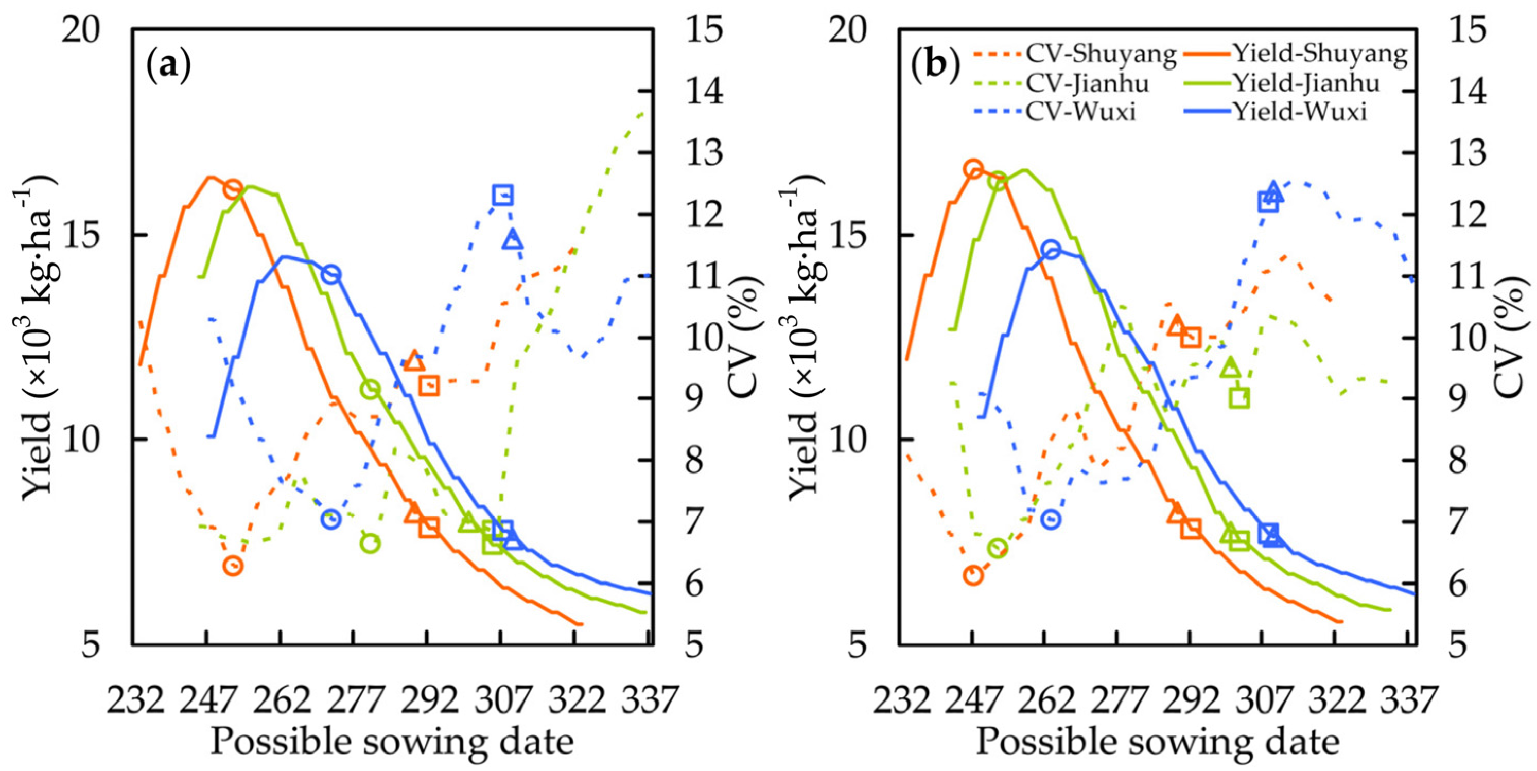
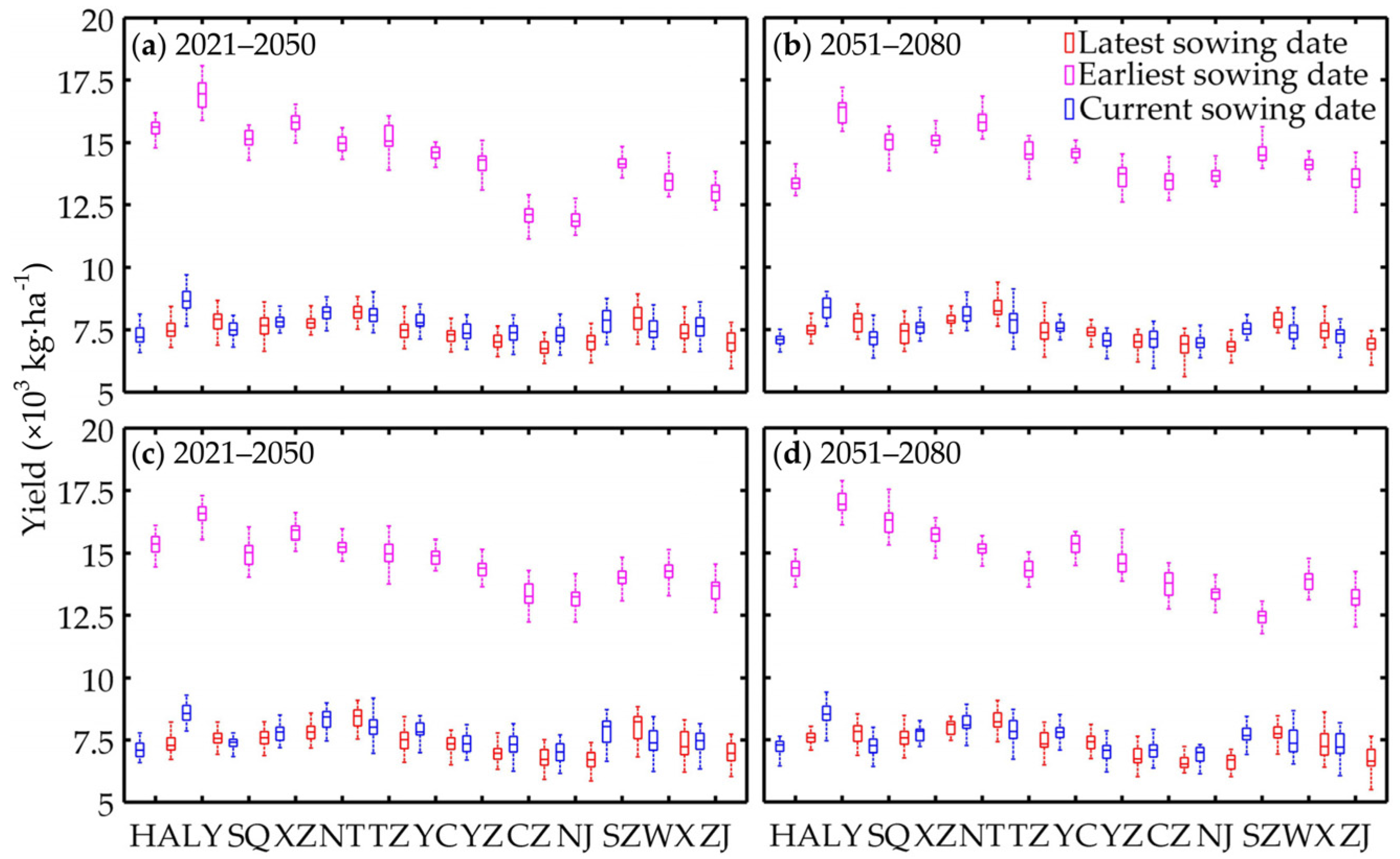
3.5. Sensitivities of the Projected Productions to the Chosen Sowing Date
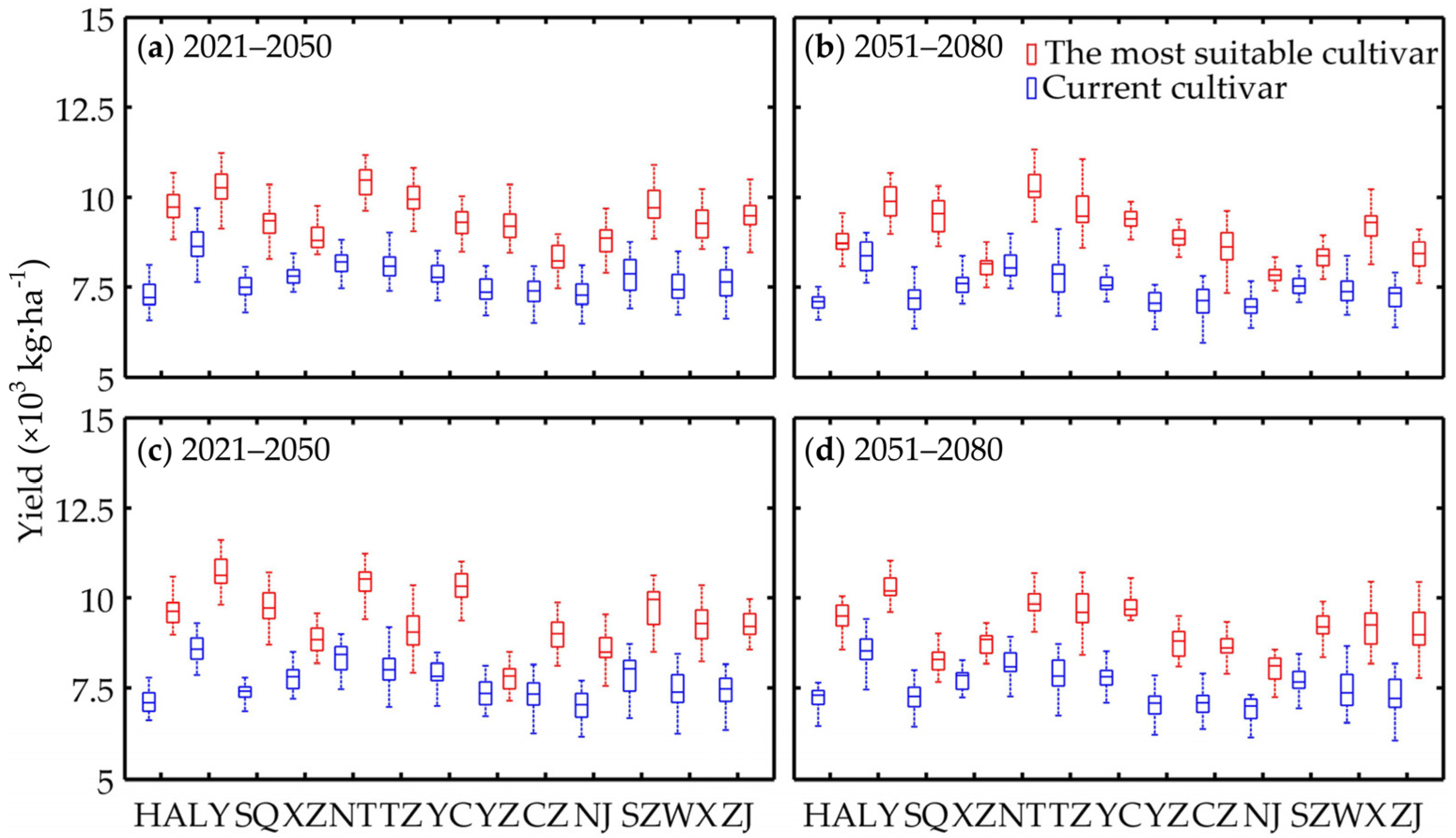
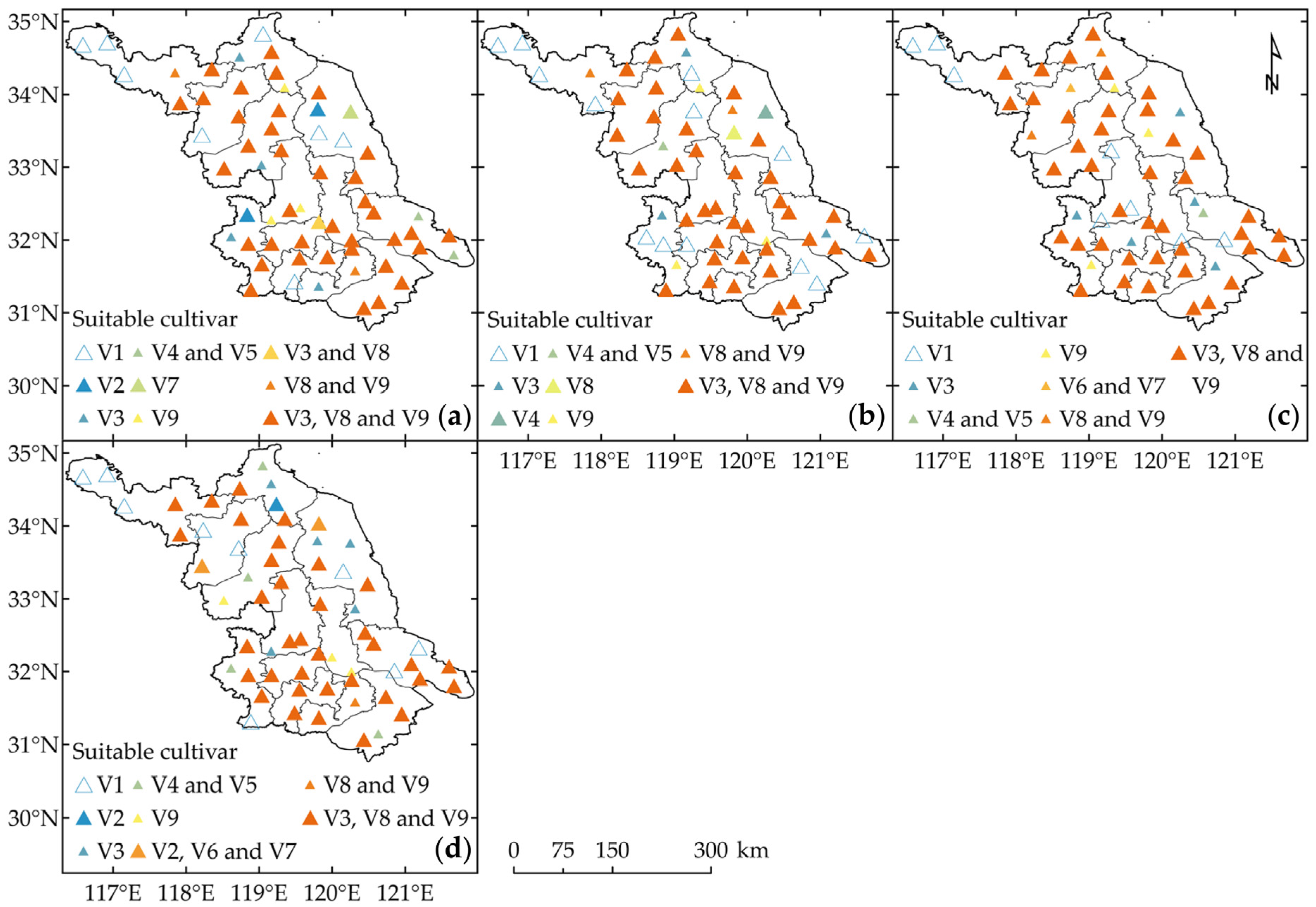
3.6. Sensitivities of the Projected Productions to the Chosen Cultivar
4. Discussion
5. Conclusions
Acknowledgments
Author Contributions
Conflicts of Interest
Appendix
A Bias Correction (BC) Method for Model-Simulated Climate Data
- (i)
- First, a nonlinear transfer function between the mean values of historical simulations and observations was determined for each ten-day period of the year. This function was constructed using a quadratic regression equation as follows:where and are the predictor and predictand, respectively. Our experiments suggested this quadratic form of transfer function because linear functions explained only a small fraction of the observed climate variability and cubic or higher order transfer functions provided poor approximations (e.g., extremely large values) for the highly oscillatory feature.
- (ii)
- Second, the mean correction was applied to the uncorrected daily value as follows:where is an intermediate variable after mean correction.
- (iii)
- Third, the parameter was used for variation correction and was determined for each ten-day period of the year because the direct application of quadratic regression models would reduce the variability between the variable and the original predictor . This parameter was determined by the intermediate variable and the mean value of the variance of the observation during the baseline conditions as follows:
- (iv)
- Finally, the variation correction was applied as follows:where is the variable after variation correction and is the final corrected value.
References
- Rosenzweig, C.; Iglesias, A.; Yang, X.B.; Epstein, P.R.; Chivian, E. Climate change and extreme weather events; implications for food production, plant diseases, and pests. Glob. Chang. Hum. Health 2001, 2, 90–104. [Google Scholar] [CrossRef]
- Tao, F.; Yokozawa, M.; Xu, Y.; Hayashi, Y.; Zhang, Z. Climate changes and trends in phenology and yields of field crops in China, 1981–2000. Agric. For. Meteorol. 2006, 138, 82–92. [Google Scholar] [CrossRef]
- Nicholls, N. Increased Australian wheat yield due to recent climate trends. Nature 1997, 387, 484–485. [Google Scholar] [CrossRef]
- Semenov, M.A.; Porter, J.R. Climatic variability and the modelling of crop yields. Agric. For. Meteorol. 1995, 73, 265–283. [Google Scholar] [CrossRef]
- Song, Y.; Chen, D.; Dong, W. Influence of climate on winter wheat productivity in different climate regions of China, 1961–2000. Clim. Res. 2006, 32, 219–227. [Google Scholar] [CrossRef]
- Vashisht, B.B.; Mulla, D.J.; Jalota, S.K.; Kaur, S.; Kaur, H.; Singh, S. Productivity of rainfed wheat as affected by climate change scenario in northeastern Punjab, India. Reg. Environ. Chang. 2013, 13, 989–998. [Google Scholar] [CrossRef]
- De Wit, A.; Duveiller, G.; Defourny, P. Estimating regional winter wheat yield with WOFOST through the assimilation of green area index retrieved from MODIS observations. Agric. For. Meteorol. 2012, 164, 39–52. [Google Scholar] [CrossRef]
- Riha, S.J.; Wilks, D.S.; Simoens, P. Impact of temperature and precipitation variability on crop model predictions. Clim. Chang. 1996, 32, 293–311. [Google Scholar] [CrossRef]
- Hulme, M.; Barrow, E.M.; Arnell, N.W.; Harrison, P.A.; Johns, T.C.; Downing, T.E. Relative impacts of human-induced climate change and natural climate variability. Nature 1999, 397, 688–691. [Google Scholar] [CrossRef]
- Semenov, M.A. Impacts of climate change on wheat in England and Wales. J. R. Soc. Interface 2009, 6, 343–350. [Google Scholar] [CrossRef] [PubMed]
- Cuculeanu, V.; Marica, A.; Simota, C. Climate change impact on agricultural crops and adaptation options in Romania. Clim. Res. 1999, 12, 153–160. [Google Scholar] [CrossRef]
- Torriani, D.; Calanca, P.L.; Schmid, S.; Beniston, M.; Fuhrer, J. Potential effects of changes in mean climate and climate variability on the yield of winter and spring crops in Switzerland. Clim. Res. 2007, 34, 59–69. [Google Scholar] [CrossRef]
- Alexandrov, V.A.; Hoogenboom, G. The impact of climate variability and change on crop yield in Bulgaria. Agric. For. Meteorol. 2000, 104, 315–327. [Google Scholar] [CrossRef]
- Luo, Q.; Bellotti, W.; Williams, M.; Wang, E. Adaptation to climate change of wheat growing in south Australia: Analysis of management and breeding strategies. Agric. Ecosyst. Environ. 2009, 129, 261–267. [Google Scholar] [CrossRef]
- Olesen, J.E.; Trnka, M.; Kersebaum, K.C.; Skjelvåg, A.O.; Seguin, B.; Peltonen-Sainio, P.; Rossi, F.; Kozyra, J.; Micale, F. Impacts and adaptation of European crop production systems to climate change. Eur. J. Agron. 2011, 34, 96–112. [Google Scholar] [CrossRef]
- Bradshaw, B.; Dolan, H.; Smit, B. Farm-level adaptation to climatic variability and change: Crop diversification in the Canadian prairies. Clim. Chang. 2004, 67, 119–141. [Google Scholar] [CrossRef]
- Xu, Z.; Yang, Z.-L. An improved dynamical downscaling method with GCM bias corrections and its validation with 30 years of climate simulations. J. Clim. 2012, 25, 6271–6286. [Google Scholar] [CrossRef]
- Xu, Z.; Yang, Z.-L. A new dynamical downscaling approach with GCM bias corrections and spectral nudging. J. Geophys. Res. 2015, 120, 3063–3084. [Google Scholar] [CrossRef]
- Huth, R. Statistical downscaling in central Europe: Evaluation of methods and potential predictors. Clim. Res. 1999, 13, 91–101. [Google Scholar] [CrossRef]
- Bakker, A.M.R.; Bessembinder, J.J.E.; de Wit, A.J.W.; van den Hurk, B.J.J.M.; Hoek, S.B. Exploring the efficiency of bias corrections of regional climate model output for the assessment of future crop yields in Europe. Reg. Environ. Chang. 2014, 14, 865–877. [Google Scholar] [CrossRef]
- Sun, W.; Huang, Y. Global warming over the period 1961–2008 did not increase high-temperature stress but did reduce low-temperature stress in irrigated rice across China. Agric. For. Meteorol. 2011, 151, 1193–1201. [Google Scholar] [CrossRef]
- Mai, M.; Zha, S.-P.; Zhu, B.; Xu, L. Agro-climatic resource zoning in Jiangsu province. Meteorol. Environ. Res. 2010, 1, 59–63. [Google Scholar]
- Ajaaj, A.A.; Mishra, A.K.; Khan, A.A. Comparison of bias correction techniques for GPCC rainfall data in semi-arid climate. Stoch. Environ. Res. Risk Assess. 2015. [Google Scholar] [CrossRef]
- Zhang, H.-F.; Zhou, S.-L.; Wu, S.-H.; Zheng, G.-H.; Hua, S.; Li, L. Temporal and spatial variation of grain production in Jiangsu province and its influencing factors. J. Nat. Resour. 2011, 26, 319–327. (In Chinese) [Google Scholar]
- Li, S.; Wheeler, T.; Challinor, A.; Lin, E.; Ju, H.; Xu, Y. The observed relationships between wheat and climate in China. Agric. For. Meteorol. 2010, 150, 1412–1419. [Google Scholar] [CrossRef]
- Van Vuuren, D.P.; Edmonds, J.; Kainuma, M.; Riahi, K.; Thomson, A.; Hibbard, K.; Hurtt, G.C.; Kram, T.; Krey, V.; Lamarque, J.-F.; et al. The representative concentration pathways: An overview. Clim. Chang. 2011. [Google Scholar] [CrossRef]
- Riahi, K.; Rao, S.; Krey, V.; Cho, C.; Chirkov, V.; Fischer, G.; Kindermann, G.; Nakicenovic, N.; Rafaj, P. RCP8.5—A scenario of comparatively high greenhouse gas emissions. Clim. Chang. 2011, 109, 33–57. [Google Scholar] [CrossRef]
- Thomson, A.M.; Calvin, K.V.; Smith, S.J.; Kyle, G.P.; Volke, A.; Patel, P.; Delgado-Arias, S.; Bond-Lamberty, B.; Wise, M.A.; Clarke, L.E.; et al. RCP4.5: A pathway for stabilization of radiative forcing by 2100. Clim. Chang. 2011, 109, 77–94. [Google Scholar] [CrossRef]
- Gao, X.J.; Wang, M.-L.; Giorgi, F. Climate change over China in the 21st century as simulated by BCC_CSM1.1-RegCM4.0. Atmos. Ocean. Sci. Lett. 2013, 6, 381–386. [Google Scholar]
- Food and Agriculture Organization of the United Nations; International Institute for Applied Systems Analysis; World Soil Information; Institute of Soil Science—Chinese Academy of Sciences; Joint Research Centre of the European Commission. Harmonized World Soil Database, version 1.0; FAO: Rome, Italy; IIASA: Laxenburg, Austria, 2008. [Google Scholar]
- Diepen, C.V.; Wolf, J.; Keulen, H.V.; Rappoldt, C. WOFOST: A simulation model of crop production. Soil Use Manag. 1989, 5, 16–24. [Google Scholar] [CrossRef]
- Boogaard, H.L.; van Diepen, C.A.; Rötter, R.P.; Cabrera, J.M.C.A.; van Laar, H.H. WOFOST 7.1: User's Guide for the WOFOST 7.1 Crop Growth Simulation Model and WOFOST Control Center 1.5; DLO Winand Staring Centre: Wageningen, The Netherlands, 1998. [Google Scholar]
- Palosuo, T.; Kersebaum, K.C.; Angulo, C.; Hlavinka, P.; Moriondo, M.; Olesen, J.E.; Patil, R.H.; Ruget, F.; Rumbaur, C.; Takáč, J.; et al. Simulation of winter wheat yield and its variability in different climates of Europe: A comparison of eight crop growth models. Eur. J. Agron. 2011, 35, 103–114. [Google Scholar] [CrossRef]
- Huang, J.; Tian, L.; Liang, S.; Ma, H.; Becker-Reshef, I.; Huang, Y.; Su, W.; Zhang, X.; Zhu, D.; Wu, W. Improving winter wheat yield estimation by assimilation of the leaf area index from Landsat TM and MODIS data into the WOFOST model. Agric. For. Meteorol. 2015, 204, 106–121. [Google Scholar] [CrossRef]
- Li, Y.; Kinzelbach, W.; Zhou, J.; Cheng, G.D.; Li, X. Modelling irrigated maize with a combination of coupled-model simulation and uncertainty analysis, in the northwest of China. Hydrol. Earth Syst. Sci. 2012, 16, 1465–1480. [Google Scholar] [CrossRef]
- Ma, H.; Huang, J.; Zhu, D.; Liu, J.; Su, W.; Zhang, C.; Fan, J. Estimating regional winter wheat yield by assimilation of time series of HJ-1 CCD NDVI into WOFOST-ACRM model with ensemble Kalman filter. Math. Comput. Model. 2013, 58, 759–770. [Google Scholar] [CrossRef]
- Diepen, C.V.; Rappoldt, C.; Wolf, J.; Keulen, H.V. Crop Growth Simulation Model WOFOST, version 4.1; Centre for World Food Studies: Wageningen, The Netherlands, 1988. [Google Scholar]
- Saxton, K.E.; Willey, P.H. The SPAW model for agricultural field and pond hydrologic simulation. In Watershed Models; Singh, V.P., Frevert, D.K., Eds.; CRC Press: Boca Raton, FL, USA, 2006; pp. 401–435. [Google Scholar]
- Ortiz, R.; Sayre, K.D.; Govaerts, B.; Gupta, R.; Subbarao, G.V.; Ban, T.; Hodson, D.; Dixon, J.M.; Ortiz-Monasterio, J.I.; Reynolds, M. Climate change: Can wheat beat the heat? Agric. Ecosyst. Environ. 2008, 126, 46–58. [Google Scholar] [CrossRef]
- Schonfeld, M.A.; Johnson, R.C.; Carver, B.F.; Mornhinweg, D.W. Water relations in winter wheat as drought resistance indicators. Crop Sci. 1988, 28, 526–531. [Google Scholar] [CrossRef]
- Piani, C.; Haerter, J.O.; Coppola, E. Statistical bias correction for daily precipitation in regional climate models over Europe. Theor. Appl. Climatol. 2010, 99, 187–192. [Google Scholar] [CrossRef]
- Song, Y.-L.; Chen, D.-L.; Liu, Y.-J.; Xu, Y. The influence of climate change on winter wheat during 2012–2100 under A2 and A1B scenarios in China. Adv. Clim. Chang. Res. 2012, 3, 138–146. [Google Scholar]
- Mo, X.; Liu, S.; Lin, Z.; Guo, R. Regional crop yield, water consumption and water use efficiency and their responses to climate change in the North China Plain. Agric. Ecosyst. Environ. 2009, 134, 67–78. [Google Scholar] [CrossRef]
- Xiao, D.; Tao, F.; Liu, Y.; Shi, W.; Wang, M.; Liu, F.; Zhang, S.; Zhu, Z. Observed changes in winter wheat phenology in the North China Plain for 1981–2009. Int. J. Biometeorol. 2013, 57, 275–285. [Google Scholar] [CrossRef] [PubMed]
- He, L.; Asseng, S.; Zhao, G.; Wu, D.; Yang, X.; Zhuang, W.; Ning, J.; Yu, Q. Impacts of recent climate warming, cultivar changes, and crop management on winter wheat phenology across the Loess Plateau of China. Agric. For. Meteorol. 2015, 200, 135–143. [Google Scholar] [CrossRef]
- Van Oort, P.A.J.; Timmermans, B.G.H.; van Swaaij, A.C.P.M. Why farmers’ sowing dates hardly change when temperature rises. Eur. J. Agron. 2012, 40, 102–111. [Google Scholar] [CrossRef]
- Southworth, J.; Pfeifer, R.A.; Habeck, M.; Randolph, J.C.; Doering, O.C.; Rao, D.G. Sensitivity of winter wheat yields in the midwestern United States to future changes in climate, climate variability, and CO2 fertilization. Clim. Res. 2002, 22, 73–86. [Google Scholar] [CrossRef]
- Cossani, C.M.; Reynolds, M.P. Physiological traits for improving heat tolerance in wheat. Plant Physiol. 2012, 160, 1710–1718. [Google Scholar] [CrossRef] [PubMed]
- Mogensen, V.O.; Jensen, H.E.; Rab, M.A. Grain yield, yield components, drought sensitivity and water use efficiency of spring wheat subjected to water stress at various growth stages. Irrig. Sci. 1985, 6, 131–140. [Google Scholar] [CrossRef]
- Xu, Y.; Guo, J.; Zhao, J.; Mu, J. Scenario analysis on the adaptation of different maize varieties to future climate change in northeast China. J. Meteorol. Res. 2014, 28, 469–480. [Google Scholar] [CrossRef]
- Semenov, M.A.; Wolf, J.; Evans, L.G.; Eckersten, H.; Iglesias, A. Comparison of wheat simulation models under climate change. II: Application of climate change scenarios. Clim. Res. 1996, 7, 271–281. [Google Scholar] [CrossRef]
- Piani, C.; Weedon, G.P.; Best, M.; Gomes, S.M.; Viterbo, P.; Hagemann, S.; Haerter, J.O. Statistical bias correction of global simulated daily precipitation and temperature for the application of hydrological models. J. Hydrol. 2010, 395, 199–215. [Google Scholar] [CrossRef]
- Olesen, J.E.; Carter, T.R.; Díaz-Ambrona, C.H.; Fronzek, S.; Heidmann, T.; Hickler, T.; Holt, T.; Minguez, M.I.; Morales, P.; Palutikof, J.P.; et al. Uncertainties in projected impacts of climate change on European agriculture and terrestrial ecosystems based on scenarios from regional climate models. Clim. Chang. 2007, 81, 123–143. [Google Scholar] [CrossRef]
- Guo, J.; Zhao, J.; Wu, D.; Mu, J.; Xu, Y. Attribution of maize yield increase in China to climate change and technological advancement between 1980 and 2010. J. Meteorol. Res. 2014, 28, 1168–1181. [Google Scholar] [CrossRef]
- Chen, R.; Ersi, K.; Yang, J.; Lu, S.; Zhao, W. Validation of five global radiation models with measured daily data in China. Energ. Convers. Manag. 2004, 45, 1759–1769. [Google Scholar] [CrossRef]


| Variety | Parameters | Characteristics |
|---|---|---|
| V1 | SPAN = 28.0 °C and DEPNR = 4.0 | Current variety |
| V2 | SPAN = 29.0 °C and DEPNR = 4.0 | Heat tolerant |
| V3 | SPAN = 30.0 °C and DEPNR = 4.0 | Heat tolerant |
| V4 | SPAN = 28.0 °C and DEPNR = 4.5 | Drought resistant |
| V5 | SPAN = 28.0 °C and DEPNR = 5.0 | Drought resistant |
| V6 | SPAN = 29.0 °C and DEPNR = 4.5 | Heat tolerant and drought resistant |
| V7 | SPAN = 29.0 °C and DEPNR = 5.0 | |
| V8 | SPAN = 30.0 °C and DEPNR = 4.5 | |
| V9 | SPAN = 30.0 °C and DEPNR = 5.0 |
| Elements | 1961–1990 | 2021–2050 | 2051–2080 | ||
|---|---|---|---|---|---|
| RCP4.5 | RCP8.5 | RCP4.5 | RCP8.5 | ||
| T (°C) | 14.77 | +0.38 | +0.42 | +0.44 | +0.63 |
| Tmax (°C) | 19.51 | +0.30 | +0.33 | +0.30 | +0.45 |
| Tmin (°C) | 11.10 | +0.38 | +0.42 | +0.49 | +0.71 |
| UV (m·s−1) | 2.97 | Increase less than 0.01 | Decrease less than 0.01 | Decrease less than 0.01 | Decrease less than 0.01 |
| P (mm) | 1578.05 | −4.50 | −0.79 | −1.12 | −6.04 |
| R (MJ·m−2) | 4641.56 | +13.86 | +15.36 | +15.08 | +12.96 |
| Variables | 1961–1990 | 2021–2050 | 2051–2080 | |||
|---|---|---|---|---|---|---|
| RCP4.5 | RCP8.5 | RCP4.5 | RCP8.5 | |||
| GS | Mean (d) | 222 | 220 | 220 | 219 | 218 |
| Standard deviation (d) | 1.21 | 1.12 | 1.37 | 1.07 | 1.31 | |
| CV (%) | 0.54 | 0.51 | 0.62 | 0.49 | 0.60 | |
| Trend (d·decade−1) | −0.48 a | −0.78 a | −0.59 a | −0.24 | −0.72 a | |
| WUE | Mean (kg·m−3) | 4.5 | 5.0 | 5.0 | 4.8 | 4.9 |
| Standard deviation (kg·m−3) | 0.117 | 0.179 | 0.174 | 0.164 | 0.178 | |
| CV (%) | 2.6 | 3.6 | 3.5 | 3.4 | 3.6 | |
| Trend (kg·decade−1·m−3) | −0.041 a | −0.046 | −0.083 a | −0.036 | 0.036 | |
| Yield | Mean (kg·ha−1) | 7239 | 7768 | 7714 | 7527 | 7613 |
| Standard deviation (kg·ha−1) | 159 | 246 | 226 | 167 | 189 | |
| CV (%) | 9.8 | 9.9 | 9.9 | 9.7 | 9.8 | |
| Trend (kg·decade−1·ha−1) | −36.4 | −75.7 | −154.4 a | −53.5 | 47.3 | |
© 2016 by the authors; licensee MDPI, Basel, Switzerland. This article is an open access article distributed under the terms and conditions of the Creative Commons by Attribution (CC-BY) license (http://creativecommons.org/licenses/by/4.0/).
Share and Cite
Tao, S.; Shen, S.; Li, Y.; Wang, Q.; Gao, P.; Mugume, I. Projected Crop Production under Regional Climate Change Using Scenario Data and Modeling: Sensitivity to Chosen Sowing Date and Cultivar. Sustainability 2016, 8, 214. https://doi.org/10.3390/su8030214
Tao S, Shen S, Li Y, Wang Q, Gao P, Mugume I. Projected Crop Production under Regional Climate Change Using Scenario Data and Modeling: Sensitivity to Chosen Sowing Date and Cultivar. Sustainability. 2016; 8(3):214. https://doi.org/10.3390/su8030214
Chicago/Turabian StyleTao, Sulin, Shuanghe Shen, Yuhong Li, Qi Wang, Ping Gao, and Isaac Mugume. 2016. "Projected Crop Production under Regional Climate Change Using Scenario Data and Modeling: Sensitivity to Chosen Sowing Date and Cultivar" Sustainability 8, no. 3: 214. https://doi.org/10.3390/su8030214
APA StyleTao, S., Shen, S., Li, Y., Wang, Q., Gao, P., & Mugume, I. (2016). Projected Crop Production under Regional Climate Change Using Scenario Data and Modeling: Sensitivity to Chosen Sowing Date and Cultivar. Sustainability, 8(3), 214. https://doi.org/10.3390/su8030214