Dynamic Coupling Analysis of Urbanization and Water Resource Utilization Systems in China

Abstract

While urbanization brings economic and social benefits, it also causes water pollution and other environmental ecological problems. This paper provides a theoretical framework to quantitatively analyze the dynamic relationship between water resource utilization and the process of urbanization. Using data from Jiangsu province, we first construct indices to evaluate urbanization and water resource utilization. We then adopt an entropy model to examine the correlation between urbanization and water resource utilization. In addition, we introduce a dynamic coupling model to analyze and predict the coupling degree between urbanization and water resource utilization. Our analyses show that pairing with rising urbanization during 2002–2014, the overall index of water resource utilization in Jiangsu province has experienced a “decline -rise-decline” trend. Specifically, after the index of water resource utilization reached its lowest point in 2004, it gradually began to rise. Water resource utilization reached its highest value in 2010. The coupling degree between urbanization and water resource utilization was relatively low in 2002 and 2003 varying between −90° and 0°. It has been rising since then. Out-of-sample forecasts indicate that the coupling degree will reach its highest value of 74.799° in 2016, then will start to gradually decline. Jiangsu province was chosen as our studied area because it is one of the selected pilot provinces for China’s economic reform and social development. The analysis of the relationship between provincial water resource utilization and urbanization is essential to the understanding of the dynamic relationship between these two systems. It also serves as an important input for developing national policies for sustainable urbanization and water resource management.

1. Introduction

Urbanization draws the rural population into cities as secondary and tertiary industries, and also develop into urban areas. As a result, the scale of urbanization expands over time [1,2]. Urbanization also reflects changes in industrialization, technological modernization, and social changes in the country [3]. In the 1800s, the world’s urban population accounted for 2.4% of the total population. By 1950, it had increased to 29.2%. The urban population then surged to 42.6% by 1990, and rising further to 50% by 2000. The global urban population is expected to reach 62.5% by 2025 [4]. Greater increasing urbanization increases the urban population, the number of cities, and also improves social wellbeing and promotes intensified uses of economic resources. Urban development is a mixture of a complex spatial morphological changes and social progress [5,6]. While urbanization brings many social and economic benefits, it can also lead to serious ecological and environmental problems caused by industrialization and dense population concentrations. With rapid urbanization, water scarcity, water pollution, and issues of water usage efficiency have become prominent problems in some Chinese areas. Potential struggles between urbanization and water conservation have clearly become an important issue [7,8,9]. Therefore, it is important to learn how to coordinate water resource utilization during urbanization process.

Urbanization and efficient water resource utilization are essential to economic development. Studies on this topic focus mainly on two aspects: first, how do water resources support and accelerate the urbanization process. Abundant water resources not only provide for the daily needs of city-dwellers, water is also an important input for various industrial and tertiary activities [10,11]. Furthermore, abundant water resources support improved ecological, environmental, and climatological factors that are attractive to business firms and talented workers. This can increase both the speed and quality of urbanization [12]. Lei and Chen [13] studied the importance of East Lake to the urbanization of Wuhan city using the water ecological carrying capacity (WECC) measure. Studying Barcelona and Madrid, March [14] considers how urbanization mobilizes water resources to keep pace with sustainable urban growth.

The second topic studied relates to changes in water resources accompanying urbanization. Urbanization is usually characterized by construction that increases impervious areas and reductions in agricultural and forest lands. This can lead to many well-known environmental problems, such as water shortages [15,16], water and air pollution [17], and the creation of urban heat islands [18]. Studies have demonstrated that degradation of river structures has created severe problems related to river health, including the “urban stream syndrome”. These problems can be particularly devastating to human development [19,20,21]. On the other hand, some remarkable improvements in water quality accompanied by urbanization in highly developed watersheds. primarily due to the influence of comprehensive water management practices (particularly for COD, BOD, NH3-N, and TP) [22]. Shrestha et al. [23] found that the Bagmati river water quality was so chemically and biologically degraded that it could not be used for any purpose due to rapid population growth and urbanization. This is particularly a problem during the region’s dry season.

While many studies focus on the linkage between urbanization and water resource utilization, few have conducted systematic analyses of the interaction between the two. In fact, urbanization itself is an integral process of urban growth and water resource utilization. All elements in these two processes function together under both social and economic restraints.

The coupling effect takes a spiraling progression from a lower degree to a higher degree of coordination [24,25,26]. In this study, we analyze the coupling effect between the evolution of urbanization and water resources utilization using data from Jiangsu province in Southeastern China. This province’s economy is booming and is highly urbanized. Its GDP in 2014 was about $10 trillion, and it was 65.2% urbanized. In addition, Jiangsu’s water system is unique: it has insufficient local water resources but abundant transit water [27]. Using the coupling model, we analyze trends associated with coordinating development between urbanization and water utilization. We further forecast the future coupling degrees between the two systems and provide some policy recommendations for sustainable urbanization in Jiangsu province. By presenting a theoretical framework and quantitative analyses of the relationship between water resources and urbanization processes in this province, we hope to provide provincial and local governments with a better understanding of the interplay of resource management and urbanization. This will assist provincial governments in implementing effective policies for sustainable water resource management as urbanization progresses.

2. Material and Methods

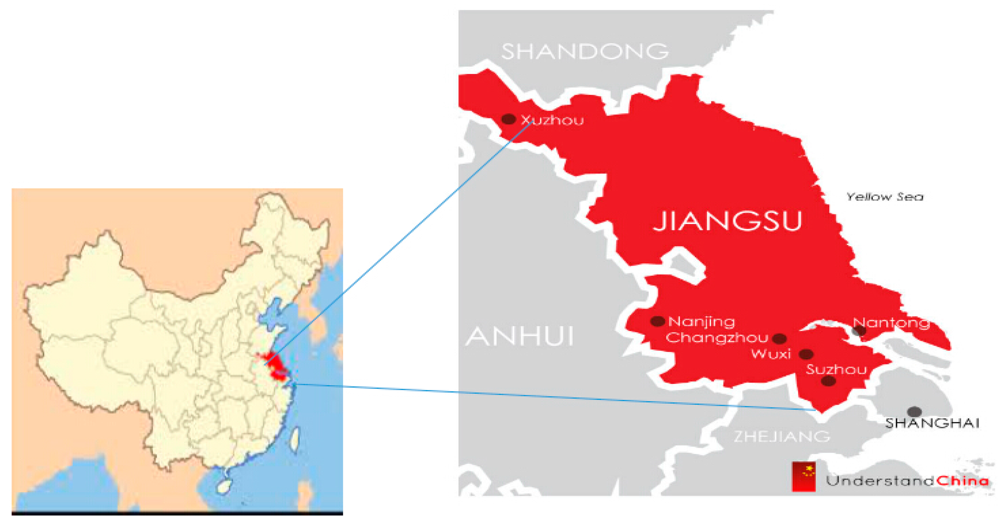
2.1. Description of Studied Area

Jiangsu province is located on the southeastern coast of China (see Figure 1). It consists of 13 cities, including Nanjing and Suzhou, covering an area of 102,600 km², accounting for 1.06 percent of China’s land mass. Jiangsu is 70,600 km² of plain with a water surface area of 17,300 km². This province’s climate is in a transition zone between subtropical and temperate. Separated by the Huaihe River and an irrigation canal, the southern part of Jiangsu is in the humid, subtropical, monsoon-climate area, while the northern part has a drier, semi-humid climate [28]. Annual precipitation gradually increases from north to south, with average annual rainfall between 700–1100 mm. Annual average sunshine hours are between 2000–2400 h. The average temperature also gradually increases from north to south, but the difference is negligible [29]. The annual average temperature is between 14–16 °C and annual average wind speed is between 2–4 m per second with relatively small regional differences.

The economy of Jiangsu province has been growing rapidly in the 21st century. GDP per capita was $1423 in 2000 growing to $13,328 by 2014. Rapid economic growth accelerated urbanization with the urban population increasing from 41.5% in 2000 to 65.2% in 2014. Employment in urban areas expanded from 6.7 million to 15.1 million between 2000 and 2014.

Water resources in Jiangsu province are unevenly distributed, both seasonally and locationally. Precipitation in the southern part is greater than the northern region with 60%–70% of the rain falling between June and September. Average annual surface water evaporation is about 950–1100 mm. Water evaporation, however, increases from southwest to the north. Most precipitation evaporates with the annual average runoff depth of about 246 mm, which is only about 2.25 percent of total rainfall. The province is located downstream of the Yangtze and Huaihe Rivers. About 1.03 trillion m³ of water flows into the province annually from these rivers. This serves as the main water source for urban residents and industries. Since the province is flat and not suitable for constructing dams or large reservoirs, it is difficult to retain transitional and local surface water. Poor capacity in regulating or storing water has led to insufficient supplies of water [30,31] with seasonal and regional water shortages often occurring in dry years.

In 2014, the total provincial water usage was 48 billion m³. The industrial and agricultural water usage was 44.2 billion m³ (92% of total water usage), domestic water usage was 3.58 billion m³ (7.4% of total water usage), and the remaining 0.6% was urban ecological and environmental usage. Compared to water usage in 2013, industrial and agricultural water usage decreased by 3.9%, while domestic usage increased by 0.8%. One serious problem with provincial water resources is water pollution. In 2014, industrial waste water totaled 2.05 billion tons, and domestic waste water reached 3.96 billion tons. To address these issues, understanding of the dynamic relationship between water resource utilization and urbanization is essential as urbanization progresses.

2.2. Methodology

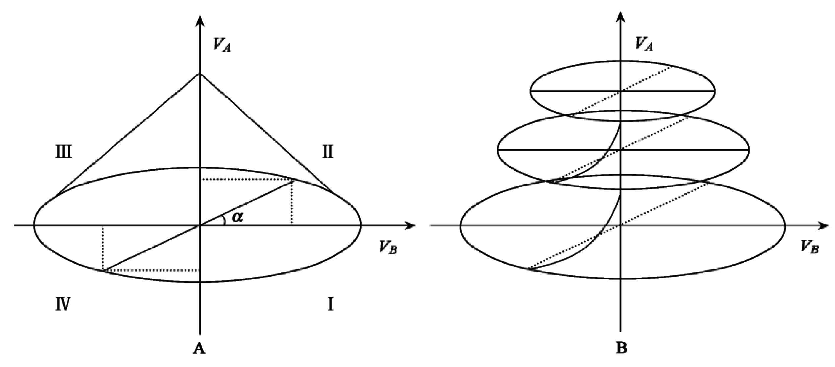
2.2.1. The Coupling Model

There is a dynamic coupling relationship between urbanization and water resource utilization. This relationship can c considered as a non-equilibrium, self-regulating, and dynamically-oscillating system [32]. This study applies the idea of systematic evolution to establish a dynamic coupling model between urbanization and water resource utilization. The progression of urbanization and water resource utilization is a nonlinear process and the evolution equation is:

$$\frac{dx(t)}{dt}=f(x_1,x_2\cdots x_n),i=1,2,\cdots ,n$$

(1)

Since the nonlinear system’s stability is mainly determined by the characteristics of the root function, we can expand Equation (1) at t = 0 as a Taylor series expansion given the system’s stability. By omitting the higher-order terms E(x₁, x₂, x_n), a linear function of the system can be approximated as:

$$\begin{array}{l}\frac{dx(t)}{dt}={\displaystyle \sum _{i=1}^n{\alpha }_i{x}_i},i=1,2,\cdots n\end{array}$$

(2)

The evolution function for urbanization and water resource utilization can be expressed as:

$$f(u)={\displaystyle \sum _{i=1}^n{\alpha }_i{x}_i,}i=1,2,\cdots n$$

(3)

$$f(w)={\displaystyle \sum _{i=1}^n{\beta }_i{y}_i,}i=1,2,\cdots n$$

(4)

where $x、y$ represent the elements of urbanization and water utilization respectively; and $\alpha 、\beta$ are their respective weights. Given the complex relationships between urbanization and water resource utilization, we transform the two systems into one comprehensive system. According to system structure theory, the evolution functions can be written as:

$$A=\frac{df(w)}{dt}=a_1{f}^{\prime }(u)+a_2{f}^{\prime }(w),V_A=\frac{dA}{dt}$$

(5)

$$B=\frac{df(u)}{dt}=b_1{f}^{\prime }(u)+b_2{f}^{\prime }(w),V_B=\frac{dB}{dt}$$

(6)

where A and B represent the dynamic evolution trend of urbanization and water resource utilization respectively, and V_A and V_B are the evolution speeds under various conditions for the two systems.

The function of the evolution speed for the comprehensive/overall system, V, can be expressed as V = F(V_A, V_B). The path of function V can be used to analyze the dynamic coupling effect between urbanization and water utilization systems.

Considering the evolution path of function V as the result of the interactions between V_A and V_B, the coordinated system can be used to analyze the evolution path of V_A and V_B as shown in Figure 2. The angle between V_A and V_B, α, represents the coupling degree of the two systems, and α satisfies tanα = V_A/V_B. By calculating α, α = arctan(V_A/V_B), the evolution trend of the overall system can be further depicted. The dynamic coupling degree between urbanization and water resources utilization is clearly presented in Figure 2.

Based on the values of the coupling degree between urbanization and water utilization, there are four stages in the coupling process shown in Panel A in Figure 2: quadrant I, coordinated symbiosis stage; quadrant II, coordinated development stage; quadrant III, limited development stage; and quadrant IV, spiral progressing stage.

In quadrant I, −90° < α < 0°, the two systems are in stage I: coordinated symbiosis. During this stage, the two systems develop independently. The urbanization process is relatively slow and water resource constraints are relatively weak. There is relatively low integration between the two systems.

In quadrant II, 0° < α < 90°, the two systems are in a coordinated development stage. With the acceleration of urbanization, problems with water shortages and pollution start to develop. Conflicts emerge between the two systems as urbanization progresses.

In quadrant III, 90° < α < 180°, the two systems are in a limited development stage. The rapid growth of urbanization further intensifies the conflicts between urbanization and water resources. With the accelerating urbanization, the demand for water resources surges sharply due to the growing demographic and economic factors. This causes serious ecological and environmental pollution and promotes misuse of water resources. This further strains the relationship between urbanization and water utilization. At this stage, the overall system may evolve into two possible scenarios: (1) conflicts between urbanization and water utilization cannot be resolved. As water shortage problems increase, the whole system collapses and civilization and its economy regress; and (2) people attempt to confront the water crisis caused by urbanization. The community can adopt effective measures to increase the local water supplies with government stringently regulating industrial and water-consuming activities to optimize water demand [33]. With continued adjustments and regulations, the internal elements of the comprehensive plan can be optimally harmonized. Then the coupling relationship between urbanization and water utilization can evolve favorably until the coupling relationship reaches the optimal symbiosis as shown in Panel B of Figure 2.

In quadrant IV, −180° < α < −90°, the coupling degree is in the rising spiral stage. As urbanization progresses, industrial and residential water usage improve and are optimized. A water-conserving society is established and enhanced. The coupling relationship between urbanization and water utilization is stabilized, and the overall system is in the rising spiral stage.

Although the four quadrants represent the entire interaction process of the two systems, it does not mean every provincial/local interaction between water resources and urbanization would experience all four quadrants. Areas/regions experiencing slow urban growth tend to stay in quadrants I and II for long periods of time. This suggests that slow urban growth does not present a threat to water resources. For rapid urbanization areas, the conflicts between urbanization and water resources may not be resolved, with the two systems in a “downward spiral” remaining in quadrant III. If the conflicts stay unresolved, it may ultimately lead to total destruction of the eco-system with the city becoming uninhabitable. Another possible development in quadrant III is that local government and residents adopt effective measures to resolve the conflicts. Then the two systems progress into quadrant IV—the coupling relationship between urbanization and water utilization is stabilized and optimized.

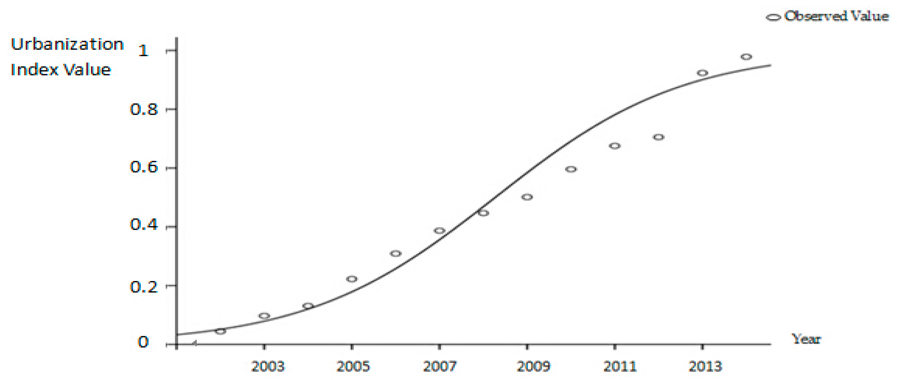
2.2.2. Forecasting Model

An exponential smoothing model is often used in forecasting time series models. It typically includes three smoothing methods: single exponential smoothing, double exponential smoothing, and triple exponential smoothing. Studies show that using triple exponential smoothing ensures superior forecasts for trended time series data [34,35], that is, the forecasts are closer to the actuals using triple exponential smoothing. Thus, we choose the triple exponential smoothing method to forecast the degrees of coupling. In triple exponential smoothing, we need to transform the original data. We first calculate the single exponential smoothing value, the double exponential smoothing value, and then the triple exponential smoothing value. Forecasts are then estimated. Suppose time series data are: X₁, X₂, X₃, …, X_n, the calculation process is as follows:

$$S_t^{(1)}=\alpha x_t+(1-\alpha )S_{t-1}^{(1)}$$

(7)

$$S_t^{(2)}=\alpha S_t^{(1)}+(1-\alpha )S_{t-1}^{(2)}$$

(8)

$$S_t^{(3)}=\alpha S_t^{(2)}+(1-\alpha )S_{t-1}^{(3)}$$

(9)

where α is the smoothing factor, and 0° < α < 1°. The smoothed statistic, S_t, is a simple weighted average of the observations X_t and the previous smoothed statistic S_t−1. S_t⁽¹⁾ is the single exponential smoothing value, S_t⁽²⁾ is the double exponential smoothing value, and S_t⁽³⁾ is the triple exponential smoothing value.

The forecasting model with triple exponential smoothing is as follows:

$$y_{t+T}=a_t+b_{t}T+c_t{T}^2$$

(10)

where Y_t+T is the forecasted value, t is the base year, T is the forecasted period, $a_t$, $b_t$, and $c_t$ are the smoothing coefficients, which are calculated as:

$$a_t=3S_t^{(1)}-3S_t^{(2)}+S_t^{(3)}$$

(11)

$$b_t=\frac{\alpha }{2{(1-\alpha )}^2}[(6-5\alpha )S_t^{(1)}-2(5-4\alpha )S_t^{(2)}+(4-3\alpha )S_t^{(3)}]$$

(12)

$$c_t=\frac{{\alpha }^2}{2{(1-\alpha )}^2}[S_t^{(1)}-2S_t^{(2)}+S_t^{(3)}]$$

(13)

2.3. Index System for Urbanization and Water Resources Utilization

2.3.1. Construction of the Urbanization Index System

Urbanization is an evolutionary process that transforms economic production and lifestyle. Studies [36,37,38,39,40] have shown that in constructing an urbanization evaluation index, four aspects should be considered: demographic, economic, social, and environmental factors. As urbanization progresses, urban population and city size continue to expand and the economic engine shifts from primary to secondary and tertiary industries. The concentration of resources and the changes in industrial structure bring rapid economic growth [36,37]. Therefore, we include the urban to total population ratio, employment ratio of tertiary industries, and urban employment ratio to account for the demographic aspect.

Urbanization improves the industrial structure and resource utilization efficiency; as a result, the local economy and household incomes grow rapidly. We adopt GDP per capita and disposable income per urban household as proxies for economic growth and the ratio of value-added by tertiary industries to reflect changes in economic structure.

The growth of the urban population and changes in economic structure promote improvement in social welfare. Urban residents desire generous transfer programs/safety net, better education services, and better medical services, hoping to improve quality of life [38,39]. Thus, we adopt four measures to reflect quality of social welfare. Social benefit expenses mainly include pensions for disabled and killed-in-action soldiers, living allowance for veterans, natural disaster relief funds, and reconstruction subsidies for post-extraordinary natural disasters. Social benefit expenses reflect the extent of financial assistance provided to the society’s most vulnerable groups by regional governments. Therefore, we include these to reflect the quality of social welfare provided by the government. Employment in the health sector (in 10,000 s) reflects the quality of medical services. The number of college students is a proxy for the quality of education services. An area with a large number of college students tends to have more universities and research institutions, which can easily lead to technological innovations and developments to provide higher quality of social welfare. We also adopt the Engel coefficient of urban households as another indicator for quality of social welfare. A small Engel coefficient indicates a relatively low level of expenditure on food and beverages by urban households. This means the expenditures on social and other activities would be relatively high, which can improve the quality of social welfare.

Urbanization brings economic and social benefits to urban dwellers, but it also carries costs, including environmental pollution. Urbanization promotes rapid growth in population and industrial output. As a result of growing population and industrial output, air pollution and industrial solid waste become serious environmental problems. In the calculation of our urbanization index, we include two environmental factors reflecting air pollution and industrial waste: sulfur dioxide emissions and comprehensive utilization rate of industrial solid waste [22,23]. Other factors, such as the ratio of urban green area to housing area, and green area per capita, are typical indicators for a positive eco-environment.

We construct our urbanization evaluation index using data from Jiangsu province. The detailed aspects of the four factors of our urbanization index are shown in

Table 1. Urbanization evaluation index system for Jiangsu province.

System Layer	Sub-System Layer	Index Layer	Weights
Urbanization	Demographic Factors	Urban population/total population	0.071
		Employment in tertiary industries/total employment	0.039
		Urban employment/total employment	0.185
		Urban population density	0.071
	Economic Factors	GDP per capita	0.071
		Value-added of the tertiary industries/total GDP	0.082
		Disposable income per urban resident	0.069
	Social Factors	Social benefits expenses	0.088
		Engel coefficient of urban households	0.038
		Employment in health sector (10,000)	0.093
		Numbers of college students	0.037
	Environmental Factors	Urban green area/housing area	0.042
		Green area per capita	0.038
		Sulfur dioxide emissions (10,000 ton)	0.040
		Comprehensive utilization rate of industrial solid waste	0.037

Source: Statistical Yearbook of Jiangsu Province [41,42,43,44,45,46,47,48,49,50,51,52,53].

.

The determinations of weights of the index system are calculated using the entropy method. This method assigns weights based on raw data and are not influenced by human factors [54]. The method first conducts an information entropy calculation using standardized index data. The formula is: $E_j=-\ln {\left(n\right)}^{-1}{\displaystyle \sum _{j=1}^n{p}_{ij}}\ln p_{ij}$, where $p_{ij}=Y_{ij}/{\displaystyle \sum _{i-1}^n{Y}_{ij}}$, and $Y_{ij}$ is the standardized index data. The weight of entropy of the jth indicator could be defined as: $W_j=\frac{1-E_j}{m-{\displaystyle \sum _{j=1}^m{E}_j}}$, in which $0\le W_j\le 1$, and ${\displaystyle \sum _{j=1}^m{W}_j}=1$. Calculated weights of urbanization index are shown in Table 1.

2.3.2. Construction of the Water Resources Utilization Index System

Water is an essential natural resource. Water shortages combined with inefficient uses of water often lead to lower water tables, degraded forests, disappearing lakes and rivers, and water pollution problems. This environmental degradation adversely affects development [55,56]. In Jiangsu province, water supply differs by location and season. Thus, the distribution, protection, and utilization of water resources can have a significant impact on regional socio-economic development [57]. Water resource utilization is a complex economic and engineering problem. We constructed a water resource utilization evaluation index for Jiangsu province based on three dimensions: volume of water resources, water utilization efficiency, and water environmental management. We include four factors to measure the volume of water resources. Three water utilization efficiency measures are included: overall, industrial, and agricultural water utilization efficiency. Four water environmental management measures are selected: industrial waste water, residential wastewater, ratio of sewage control to total pollution control investment, and the industrial wastewater compliance rate. The weight of each index layer is calculated using the same entropy method described above.

Table 2. Evaluation index system of water resource utilization.

System Layer	Sub-System Layer	Index Layer	Weights
Water Resources Utilization Index	Volume of Water Resources	Total volume of water resources (100 million m3)	0.062
		Water resources per capita	0.078
		Total volume of production water (100 million m3)	0.124
		Total volume of residential water (100 million m3)	0.114
	Water Utilization Efficiency	Water usage per 10,000 GDP (m3/10,000 yuan)	0.177
		Water usage per unit of industrial value-added (m3/10,000 yuan)	0.064
		Irrigation water usage per acre of agricultural land	0.038
	Water Environmental Management	Industrial wastewater emissions (100 million tons)	0.076
		Urban residential wastewater emission (100 million tons)	0.099
		Sewage control investment/total pollution control investment	0.120
		Industrial wastewater discharge compliance rate	0.049

Sources: Data for water resources volumes and water utilization efficiency are from “Jiangsu Water Resources Bulletin” [58,59,60,61,62,63,64,65,66,67,68,69,70]. Data for water environmental management is from the “Jiangsu Environment Protection Bulletin” [71,72,73,74,75,76,77,78,79,80,81,82,83].

shows the factors for each aspect and their respective weights.

2.3.3. Data Standardization

The data for evaluating the water resources utilization index was not available until 2002, therefore, we collected data for the period of 2002–2014.

Since the properties of the two indices are not the same, their dimensions and magnitudes also differ. We use the min-max standardizing method to normalize the data. The formulas are as follows:

$$Y_{ij}=\frac{x_{ij}-min\left(x_j\right)}{max\left(x_j\right)-min\left(x_j\right)}$$

(14)

$$Y_{ij}=\frac{max\left(x_j\right)-x_{ij}}{max\left(x_j\right)-min\left(x_j\right)}$$

(15)

where X_ij is the initial value of the jth factor at year i. Y_ij represents the corresponding standardized data. For positive data, we use Equation (14) to normalize it; for negative data, Equation (15) is used. The values of normalized data are between 0 and 1.

3. Discussion

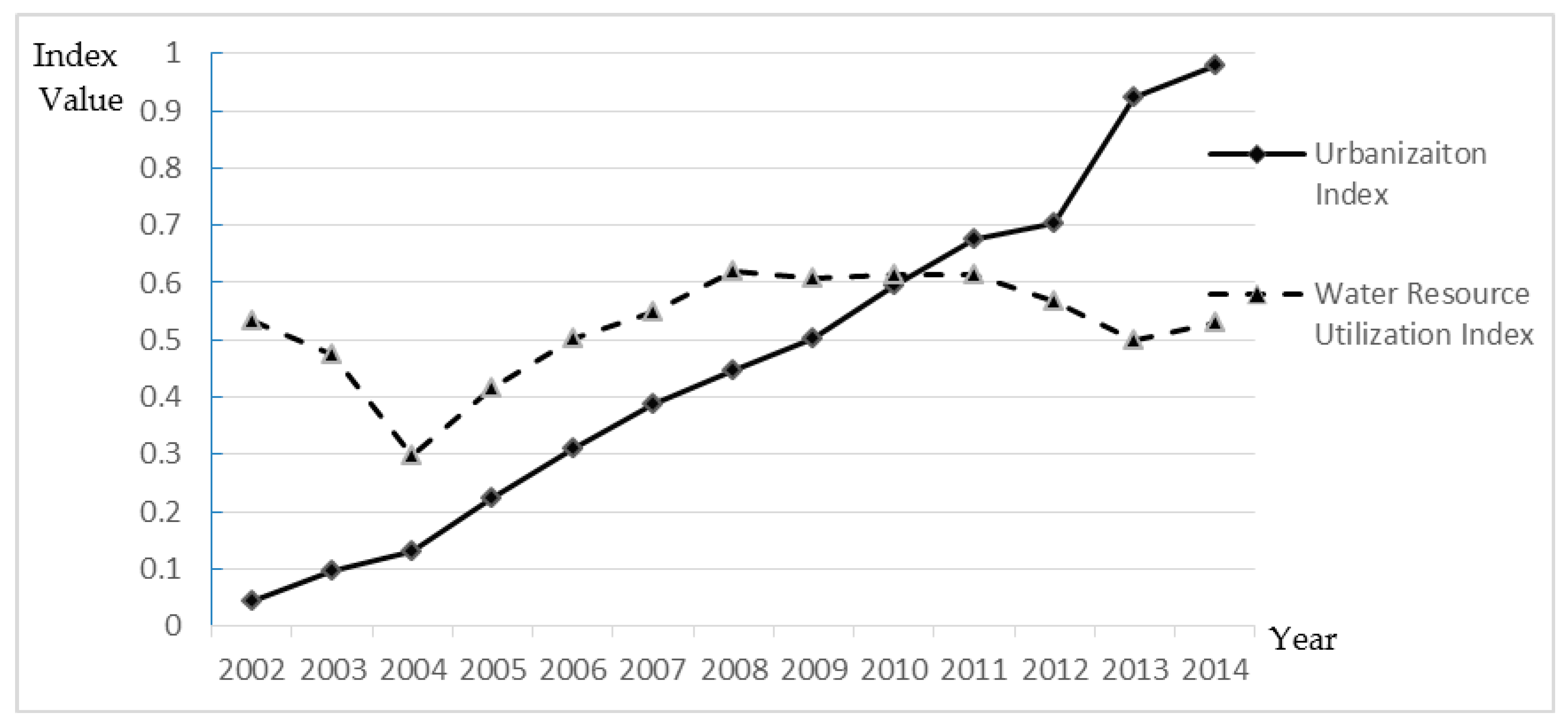
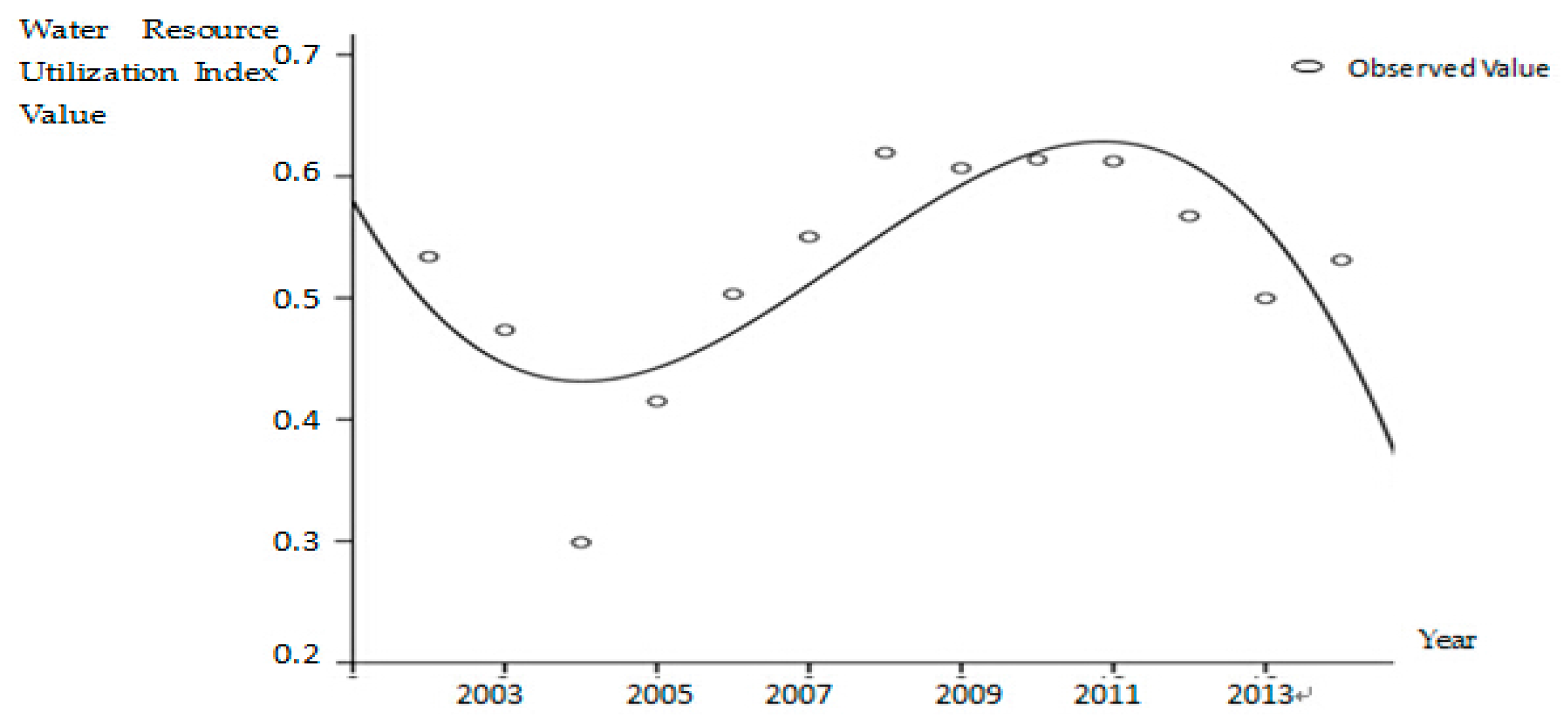
3.1. The Index of the Water Resource Utilization System for Jiangsu Province

Table 2 provides the weights for calculating the water resources utilization index. According to Table 2, the two most important factors affecting the water resources utilization index in Jiangsu are water usage per 10,000 GDP (with a weight of 0.177) and the total volume of production/industrial water (with a weight of 0.124). This means that the water usage per 10,000 GDP and production water demand are the two most important factors in evaluating water resource utilization in Jiangsu province. The computed indices are shown in Figure 3.

According to Figure 3, the index of urbanization is rising throughout the sample period, while the index of water resources utilization in Jiangsu province experienced a pattern of decline-increase-decline. The index of water utilization reached its lowest point in 2004 (0.299). It then gradually improved and reached its highest value in 2010 (0.614) after which it started to decline. There are three possible explanations for the high value in 2010: first, the total volume of production/industrial water reached the highest value, 51.5 billion m³. Second, after the “2007 Oxygenation Crisis of Taihu Lake”, the provincial government significantly increased investment in managing water pollution and improving water resources utilization. As a result, the ratio of sewage to total pollution control investment reached a high value of 0.4, it then gradually declined to 0.219 in 2014. Third, industrial wastewater discharge compliance rate was the highest for the sample period, 98.03%. This rate started to decline after 2010.

The pattern of the water utilization index can be approximated with a nonlinear fitting process as shown in Equation (10). We find that the cubic function has the best fit as shown in Equation (16) and Figure 4. The summary statistic for the regression is as follow: R² = 0.891, F value = 24.439, the t statistics for the coefficients are 5.666, −2.181, −3.585, and 3.302, respectively; all are significant at the 5% level.

$$f\left(w\right)=0.47-0.108t+0.027t^2-0.001t^3$$

(16)

3.2. The Index of Urbanization in Jiangsu Province

Among the 14 factors affecting the urbanization index in Table 1, the two most factors are urban employment ratio and employment in the health sector, with weights of 0.185 and 0.093 respectively. This indicates that the urban employment share and urban health environment are most important in computing the urbanization index for Jiangsu province.

The computed index of urbanization is depicted in Figure 3. According to this index, urbanization in Jiangsu province has increased markedly, resulting from rapid economic growth and increased industrial production. In 2002, the index of urbanization was only 0.044, but had reached 0.978 by 2013. The urbanization process of Jiangsu province has been much faster than that of other provinces in China. One of the major drivers for this has been provincial government policies. On 1 May 2003, Jiangsu implemented a “unified household registration” policy. It abolished separate registrations for agricultural residents and non-agricultural residents. The provincial government also relaxed regulations for migrant workers. Anyone with a legal local residency or a steady job in the province was allowed to apply for urban household registration. These policies drew many talented workers to the province, thus speeding up the provincial urbanization after 2003. In addition, the provincial government introduced the “urban planning template in Jiangsu Province (2012–2030)” in 2012 to help develop an affluent society and to promote sustainable urbanization. As a result the urbanization index jumped from 0.705 in 2011 to 0.923 in 2013.

Studies have shown that many regional urbanization trends can be approximated with the S-curve [84,85]. We adopt a logistic curve to fit the pattern of urbanization index. The results show the logistic curve is good fit (R² = 0.93, F value = 146.444) as shown in Equation (17) and Figure 5. The t values for the two coefficients are 5.490 and 43.579 respectively, and both are significant at 1% level. Equation (17) can be transformed into Equation (18), which is used to compute the forecasted index of urbanization:

$$\ln (1/f(u)-1)=\ln 29.62+\ln 0.627\times t$$

(17)

$$B=f(u)=\frac{1}{1+e^{\ln 29.62+\ln 0.627\times t}}$$

(18)

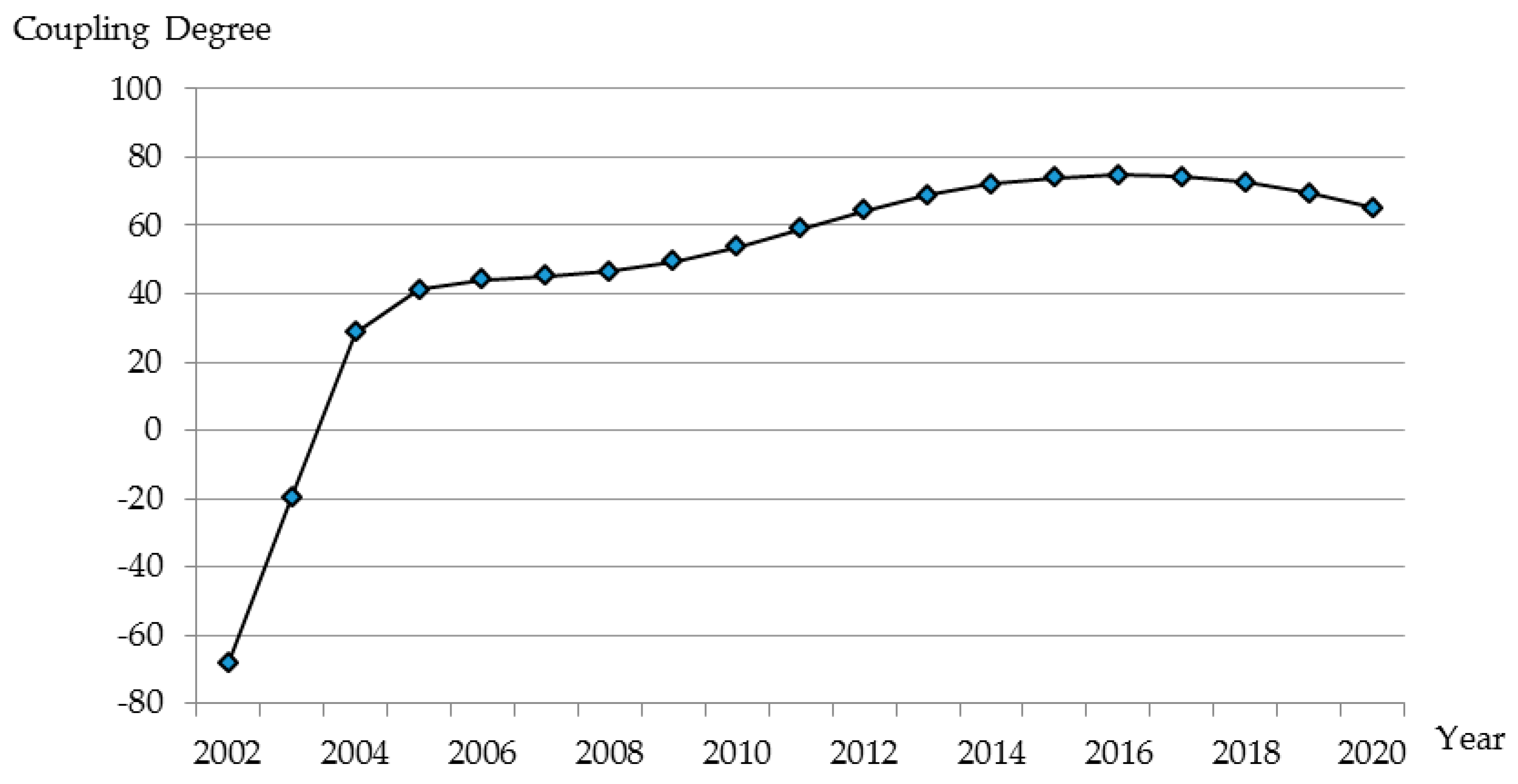
3.3. Coupling Analysis

Taking the derivative with respect to time, t, in Equations (17) and (18), we can obtain evolution equations for urbanization and water resources utilization:

$$V_A=df(w)/dt=-0.108+0.054t-0.003t^2$$

(19)

$$V_B=df(u)/dt=-\frac{\ln 0.627\times e^{\ln 29.62+\ln 0.627\times t}}{{(1+e^{\ln 29.62+\ln 0.627\times t})}^2}$$

(20)

Based on Equations (19) and (20), we calculate the values of V_A and V_B. The variable α and tanα can be calculated using formula: α = arctan(V_A/V_B). The computed annual values of V_A, V_B, α, and tanα are shown in

Table 3. The coupling statistics between urbanization and water resources utilization for Jiangsu province: 2002–2014.

Year	VA	VB	tanα	α	Quadrant
2002	−0.057	0.023	−2.519	−68.344°	I
2003	−0.012	0.034	−0.353	−19.441°	I
2004	0.027	0.049	0.546	28.630°	II
2005	0.06	0.069	0.874	41.138°	II
2006	0.087	0.089	0.973	44.205°	II
2007	0.108	0.107	1.008	45.218°	II
2008	0.123	0.116	1.058	46.609°	II
2009	0.132	0.113	1.165	49.365°	II
2010	0.135	0.099	1.359	53.645°	II
2011	0.132	0.079	1.661	58.948°	II
2012	0.123	0.059	2.084	64.364°	II
2013	0.108	0.041	2.604	68.991°	II
2014	0.087	0.028	3.104	72.143°	II

.

Table 3 and Figure 6 show that the pattern of the coupling process between urbanization and water resource utilization includes two phases. The first phase covers 2002–2003, the coupling degree was in quadrant I, −90° < α < 0°, and the two systems are in the coordinated symbiosis stage. At this stage, the level of water resource utilization declined slightly, while urbanization had just started. The interaction between the two systems was not very pronounced.

The second phase covers the years from 2004–2014, when the coupling degree was in quadrant II, 0° < α < 90°, the coordinated development stage. The coupling degree itself was rising but at a relatively slow rate. To better analyze this second phase, we further divide it into two stages. During the earlier stage, years from 2004–2007, the coupling degree rose from 28.63° to 45.218° in which the speed of urbanization far exceeded the evolution rate of water utilization. This resulted in water shortages and water pollution problems. Water resource problems became so bad that they started to threaten the urbanization process. The “2007 Oxygenation Crisis of Taihu Lake” is a notorious example of water crisis caused by rapid urbanization. The “Oxygenation Crisis of Taihu Lake” occurred in May of 2007. The environmental pollution of Taihu Lake was caused by increasing urban residential waste water and industrial waste water (two factors in water utilization index). The severe pollution led to the cyanobacteria outbreak in the lake. Seriously polluted Taihu Lake water caused 70% of the city water pollution in Wuxi city. Sheng [86] estimated that this crisis affected the drinking water supply of two million residents in Eastern China and resulted in direct economic losses of more than $30 billion.

The second stage covers 2008–2014, the coupling degree further rose from 46.609° to 72.143°. During this stage, urbanization progressed at a slower pace. In addition, following the Oxygenation Crisis in 2007, people became more environmentally conscientious and the provincial government rigorously implemented an industrial restructuring program and closed many chemical plants. Both contributed to the increase in the degree of coupling between urbanization and water resource utilization.

3.4. Forecasting the Coupling Degree

The forecast accuracy of the exponential smoothing method depends on the value of α [87]. Thus, we compare forecasted coupling degrees using three values of α.

Table 4. Forecasted coupling degrees with various values of α (t = 2007).

Year	Actual Value	α
		0.7	0.8	0.9
2012	64.364°	64.682°	65.335°	65.398°
		(0.101)	(0.941)	(1.068)
2013	68.991°	70.535°	70.491°	70.194°
		(2.383)	(2.249)	(1.447)
2014	72.143°	74.085°	73.609°	73.158°
		(3.771)	(2.151)	(1.031)
Total Squared Errors		(6.255)	(5.341)	(3.546)

Numbers in parenthesis are squared forecasting errors.

shows the predicted coupling degrees and corresponding squared errors of three values of α.

Given the values of α, the corresponding mean squared errors (MSE) are calculated as follows:

$$\begin{array}{l}{E}_t=6.255/3=2.085(\alpha =0.7)\\ E_t=5.341/3=1.780(\alpha =0.8)\\ E_t=3.546/3=1.182(\alpha =0.9)\end{array}$$

The mean squared errors indicate that the gap between forecasts and actuals is minimized when the smoothing factor α = 0.9. Therefore we adopt smoothing factor α = 0.9.

Taking year 2014 as the first period t, we calculate the smoothing coefficient $a_t$, $b_t$, and $c_t$ according to Equations (11)–(13).

$$\begin{array}{ccccccc}{a}_t=72.144& & & b_t=2.562& & & c_t=-0.617\end{array}$$

Based on Equation (10) and the values of a_t, b_t, and c_t, the forecast equation can be written as:

$$y_{t+T}=72.144+2.562T–0.617T^2$$

(21)

where T represents years. The predicted coupling degrees using Equation (21) for the period of 2015 to 2020 are shown in

Table 5. The forecasted coupling degree, years 2015–2020.

Year	2015	2016	2017	2018	2019	2020
Coupling Degree	74.088°	74.799°	74.276°	72.519°	69.528°	65.304°

.

Figure 6 plots data from Table 3 (the actual coupling degrees for years 2002–2014) and Table 5 (forecasted coupling degrees for years 2015–2020). The forecasted coupling degrees between urbanization and water resources utilization for Jiangsu province exhibit an “increase-decrease” pattern. The coupling degree is predicted to reach its highest value 74.799° in 2016, then forecast to decline. As shown in Figure 6, the pattern of coupling degrees consists of two turning points: one in 2004 and the other for the forecast value in 2016. Prior to 2004, the coupling degree between urbanization and water resources utilization increased rapidly and stayed in quadrant I. Since 2004, the coupling degree increased gradually and is predicated to peak in 2016. All predicted coupling degrees stay in quadrant II, which means the two systems are expected to stay in the coordinated development stage during the forecast period. Thus, the demand for water resources will increase to facilitate the rapid urban, economic, and social advancements. These developments will eventually cause major problems with water shortages and water pollution. Such water crises will further hinder sustainable urbanization and aggravate conflicts between urbanization and efficient water utilization. However, as people become more environmentally conscientious, they will try to optimize the tradeoff between urbanization and water resource management. Unless such changes occur, the challenge of allowing both to achieve optimal levels will remain.

4. Conclusions

This paper provides a theoretical framework analyzing the dynamic relationship between water resources utilization and the process of urbanization. We empirically examine this dynamic relationship using data from Jiangsu province in China. The results serve as an important input for developing sustainable water resource management policies during the urbanization process.

The coupling process between urbanization and water resource utilization not only reflects the complex and nonlinear interactions among various factors of two index systems, it also exhibits evolutionary phases and patterns. Based on our constructed evaluation index system, we analyze the coupling degrees of urbanization and water resources utilization in Jiangsu province. We also forecast the coupling degree of the two systems for the next six years using a cubic exponential smoothing model. Regarding the urbanization process, we find that industrial restructuring and economic development in Jiangsu province sped up the progress of urbanization. In 2002 the level of urbanization was only 0.044, but it reached 0.978 by 2013. Our analyses show the coupling degrees between urbanization and water utilization exhibit a pattern of “decline–rise–decline” for the sample period of 2002–2014. The coupling degree reached its lowest point in 2004 with the value of 0.299. Then it began to rise gradually and reached its highest value in 2010. We further divided the coupling effect between urbanization and water resource utilization into two phases. During the first phase, from 2002–2003, the two systems were at a low coordinated stage and the coupling degree stayed in quadrant I, where −90° < α < 0°. The second phase, 2004–2014, was characterized by the rising coupling degree and evident conflicts between the two systems. The coupling degree during phase two stayed in quadrant II, 0° < α < 90°. In addition, we forecast the coupling degree between these two systems. Our forecasts indicate that the coupling degree will reach its peak in 2016, and after that it starts to gradually decline. We believe that policy-makers could take our results into consideration and focus on optimizing the advancement of urbanization and sustainable management of water resources to achieve a coordinated development stage for urbanization and water resource utilization.

Possible future research could include using the theoretical framework of this study to analyze coupling degrees between urbanization and water resources utilization of other Chinese provinces. The results of such analyses would help in designing policies that coordinate urbanization and sustainable water utilization. Additional work incorporating more factors in computing the water utilization index and urbanization index would improve the quality of indices and study results. For example, adding factors to reflect the quality of urban life for the urbanization index and incorporating factors, such as ecological/environmental water usage, in computing the water utilization index.

References

1. Davis, J.C.; Henderson, J.V. Evidence on the Political Economy of the Urbanization Process. J. Urban Econ. 2003, 53, 98–125. [Google Scholar] [CrossRef]
2. Henderson, V. The Urbanization Process and Economic Growth: The So-What Question. J. Econ. Growth 2003, 8, 47–71. [Google Scholar] [CrossRef]
3. McGee, T.G. The Urbanization Process in the Third World; G. Bell and Sons, Ltd.: London, UK, 1971. [Google Scholar]
4. Zhang, J. Urbanization, Population Transition, and Growth. Oxf. Econ. Pap. 2002, 54, 91–117. [Google Scholar] [CrossRef]
5. Vermeulen, L.C.; De Kraker, J.; Hofstra, N.; Kroeze, C.; Medema, G. Modelling the Impact of Sanitation, Population Growth and Urbanization on Human Emissions of Cryptosporidium to Surface Waters—A Case Study for Bangladesh and India. Environ. Res. Lett. 2015, 10, 094017. [Google Scholar] [CrossRef]
6. Loorbach, D.; Shiroyama, H. The Challenge of Sustainable Urban Development and Transforming Cities. In Governance of Urban Sustainability Transitions; Springer: New York, NY, USA, 2016; pp. 3–12. [Google Scholar]
7. Feng, L.; Chen, B.; Hayat, T.; Alsaedi, A.; Ahmad, B. The Driving Force of Water Footprint under the Rapid Urbanization Process: A Structural Decomposition Analysis for Zhangye City in China. J. Clean. Prod. 2015. [Google Scholar] [CrossRef]
8. Bao, C.; Fang, C.-L. Water Resources Constraint Force on Urbanization in Water Deficient Regions: A Case Study of the Hexi Corridor, Arid Area of Nw China. Ecol. Econ. 2007, 62, 508–517. [Google Scholar] [CrossRef]
9. Ma, H.; Shi, C.; Chou, N.-T. China’s Water Utilization Efficiency: An Analysis with Environmental Considerations. Sustainability 2016, 8, 516. [Google Scholar] [CrossRef]
10. Xu, C.; Wang, S.; Zhou, Y.; Wang, L.; Liu, W. A Comprehensive Quantitative Evaluation of New Sustainable Urbanization Level in 20 Chinese Urban Agglomerations. Sustainability 2016, 8, 91. [Google Scholar] [CrossRef]
11. Ren, W.; Zhong, Y.; Meligrana, J.; Anderson, B.; Watt, W.E.; Chen, J.; Leung, H.-L. Urbanization, Land Use, and Water Quality in Shanghai: 1947–1996. Environ. Int. 2003, 29, 649–659. [Google Scholar] [CrossRef]
12. Hubacek, K.; Guan, D.; Barrett, J.; Wiedmann, T. Environmental Implications of Urbanization and Lifestyle Change in China: Ecological and Water Footprints. J. Clean. Prod. 2009, 17, 1241–1248. [Google Scholar] [CrossRef]
13. Ding, L.; Chen, K.-L.; Cheng, S.-G.; Wang, X. Water Ecological Carrying Capacity of Urban Lakes in the Context of Rapid Urbanization: A Case Study of East Lake in Wuhan. Phys. Chem. Earth Parts A/B/C 2015, 89, 104–113. [Google Scholar] [CrossRef]
14. March, H. Taming, Controlling and Metabolizing Flows: Water and the Urbanization Process of Barcelona and Madrid (1850–2012). Eur. Urban Reg. Stud. 2015, 22, 350–367. [Google Scholar] [CrossRef]
15. McDonald, R.I.; Green, P.; Balk, D.; Fekete, B.M.; Revenga, C.; Todd, M.; Montgomery, M. Urban Growth, Climate Change, and Freshwater Availability. Proc. Natl. Acad. Sci. USA 2011, 108, 6312–6317. [Google Scholar] [CrossRef] [PubMed]
16. Li, E.; Endter-Wada, J.; Li, S. Characterizing and Contextualizing the Water Challenges of Megacities. JAWRA J. Am. Water Resour. Assoc. 2015, 51, 589–613. [Google Scholar] [CrossRef]
17. O’Driscoll, M.; Clinton, S.; Jefferson, A.; Manda, A.; McMillan, S. Urbanization Effects on Watershed Hydrology and in-Stream Processes in the Southern United States. Water 2010, 2, 605–648. [Google Scholar] [CrossRef]
18. Zhou, D.; Zhao, S.; Zhang, L.; Sun, G.; Liu, Y. The Footprint of Urban Heat Island Effect in China. Sci. Rep. 2015, 5. [Google Scholar] [CrossRef] [PubMed]
19. Elias, E.; Dougherty, M.; Srivastava, P.; Laband, D. The Impact of Forest to Urban Land Conversion on Streamflow, Total Nitrogen, Total Phosphorus, and Total Organic Carbon Inputs to the Converse Reservoir, Southern Alabama, USA. Urban Ecosyst. 2013, 16, 79–107. [Google Scholar] [CrossRef]
20. Paul, M.J.; Meyer, J.L. Streams in the Urban Landscape. In Urban Ecology; Springer: New York, NY, USA, 2008; pp. 207–231. [Google Scholar]
21. Sun, G.; Lockaby, B.G. Water Quantity and Quality at the Urban–Rural Interface. In Urban–Rural Interfaces: Linking People and Nature; American Society of Agronomy, Soil Science Society of America, Crop Science Society of America, Inc.: Madison, WI, USA, 2012; pp. 29–48. [Google Scholar]
22. Zhao, W.; Zhu, X.; Sun, X.; Shu, Y.; Li, Y. Water Quality Changes in Response to Urban Expansion: Spatially Varying Relations and Determinants. Environ. Sci. Pollut. Res. 2015, 22, 16997–17011. [Google Scholar] [CrossRef] [PubMed]
23. Shrestha, R.A.; Huang, X.; Sillanpää, M. Effects of Urbanization on Water Quality of the Bagmati River in Kathmandu Valley, Nepal. Stud. Orient. Electron. 2015, 109, 141–150. [Google Scholar]
24. Srinivasan, V.; Lambin, E.; Gorelick, S.; Thompson, B.; Rozelle, S. The Nature and Causes of the Global Water Crisis: Syndromes from a Meta-Analysis of Coupled Human-Water Studies. Water Resour. Res. 2012, 48. [Google Scholar] [CrossRef]
25. Wu, P.; Tan, M. Challenges for Sustainable Urbanization: A Case Study of Water Shortage and Water Environment Changes in Shandong, China. Procedia Environ. Sci. 2012, 13, 919–927. [Google Scholar] [CrossRef]
26. Giacomoni, M.; Kanta, L.; Zechman, E.M. Complex Adaptive Systems Approach to Simulate the Sustainability of Water Resources and Urbanization. J. Water Resour. Plan. Manag. 2013, 139, 554–564. [Google Scholar] [CrossRef]
27. Gu, X.; Wang, Y.; Zhao, H.; Wang, F.; Zhu, X.; Lu, G. Linking between Water Resources Utilization and Economic Growth in Jiangsu Province. China Environ. Sci. 2012, 32, 351–358. [Google Scholar]
28. Wang, J.; Huang, X.; Zhong, T.; Chen, Z. Climate Change Impacts and Adaptation for Saline Agriculture in North Jiangsu Province, China. Environ. Sci. Policy 2013, 25, 83–93. [Google Scholar] [CrossRef]
29. Shuai, J.; Zhang, Z.; Liu, X.; Chen, Y.; Wang, P.; Shi, P. Increasing Concentrations of Aerosols Offset the Benefits of Climate Warming on Rice Yields During 1980–2008 in Jiangsu Province, China. Reg. Environ. Chang. 2013, 13, 287–297. [Google Scholar] [CrossRef]
30. Tao, H.; Fischer, T.; Zeng, Y.; Fraedrich, K. Evaluation of Trmm 3b43 Precipitation Data for Drought Monitoring in Jiangsu Province, China. Water 2016, 8, 221. [Google Scholar] [CrossRef]
31. Duan, H.; Hu, Q. Local Officials' Concerns of Climate Change Issues in China: A Case from Jiangsu. J. Clean. Prod. 2014, 64, 545–551. [Google Scholar] [CrossRef]
32. Fang, C.-L.; Huang, J.-C.; Bu, W.-N. Theoretical Study on Urbanization Process and Ecological Effect with the Restriction of Water Resource in Arid Area of Northwest China. Arid Land Geogr. 2004, 27, 1–7. [Google Scholar]
33. Owen, D. Urbanization, Water Quality, and the Regulated Landscape. Univ. Colo. Law Rev. 2011, 82, 431. [Google Scholar] [CrossRef]
34. Jašek, R.; Szmit, A.; Szmit, M. Usage of Modern Exponential-Smoothing Models in Network Traffic Modelling. In Nostradamus 2013: Prediction, Modeling and Analysis of Complex Systems; Springer: New York, NY, USA, 2013; pp. 435–444. [Google Scholar]
35. Yang, D.; Sharma, V.; Ye, Z.; Lim, L.I.; Zhao, L.; Aryaputera, A.W. Forecasting of Global Horizontal Irradiance by Exponential Smoothing, Using Decompositions. Energy 2015, 81, 111–119. [Google Scholar] [CrossRef]
36. Knox, P.L.; McCarthy, L. Urbanization: An Introduction to Urban Geographyr; Pearson Boston: Boston, MA, USA, 2012. [Google Scholar]
37. Brenner, N. Theses on Urbanization. Public Cult. 2013, 25, 85–114. [Google Scholar] [CrossRef]
38. Buhaug, H.; Urdal, H. An Urbanization Bomb? Population Growth and Social Disorder in Cities. Glob. Environ. Chang. 2013, 23, 1–10. [Google Scholar] [CrossRef]
39. Sato, Y.; Zenou, Y. How Urbanization Affect Employment and Social Interactions. Eur. Econ. Rev. 2014, 75, 131–155. [Google Scholar] [CrossRef]
40. Hansel, B.; Thomas, F.; Pannier, B.; Bean, K.; Kontush, A.; Chapman, M.J.; Guize, L.; Bruckert, E. Relationship between Alcohol Intake, Health and Social Status and Cardiovascular Risk Factors in the Urban Paris-Ile-De-France Cohort: Is the Cardioprotective Action of Alcohol a Myth? Eur. J. Clin. Nutr. 2010, 64, 561–568. [Google Scholar] [CrossRef] [PubMed]
41. Jiangsu Province Statistics Bureau. Statistical Yearbook of Jiangsu Province; Jiangsu Statistics Press: Nanjing, China, 2002. [Google Scholar]
42. Jiangsu Province Statistics Bureau. Statistical Yearbook of Jiangsu Province; Jiangsu Statistics Press: Nanjing, China, 2003. [Google Scholar]
43. Jiangsu Province Statistics Bureau. Statistical Yearbook of Jiangsu Province; Jiangsu Statistics Press: Nanjing, China, 2004. [Google Scholar]
44. Jiangsu Province Statistics Bureau. Statistical Yearbook of Jiangsu Province; Jiangsu Statistics Press: Nanjing, China, 2005. [Google Scholar]
45. Jiangsu Province Statistics Bureau. Statistical Yearbook of Jiangsu Province; Jiangsu Statistics Press: Nanjing, China, 2006. [Google Scholar]
46. Jiangsu Province Statistics Bureau. Statistical Yearbook of Jiangsu Province; Jiangsu Statistics Press: Nanjing, China, 2007. [Google Scholar]
47. Jiangsu Province Statistics Bureau. Statistical Yearbook of Jiangsu Province; Jiangsu Statistics Press: Nanjing, China, 2008. [Google Scholar]
48. Jiangsu Province Statistics Bureau. Statistical Yearbook of Jiangsu Province; Jiangsu Statistics Press: Nanjing, China, 2009. [Google Scholar]
49. Jiangsu Province Statistics Bureau. Statistical Yearbook of Jiangsu Province; Jiangsu Statistics Press: Nanjing, China, 2010. [Google Scholar]
50. Jiangsu Province Statistics Bureau. Statistical Yearbook of Jiangsu Province; Jiangsu Statistics Press: Nanjing, China, 2011. [Google Scholar]
51. Jiangsu Province Statistics Bureau. Statistical Yearbook of Jiangsu Province; Jiangsu Statistics Press: Nanjing, China, 2012. [Google Scholar]
52. Jiangsu Province Statistics Bureau. Statistical Yearbook of Jiangsu Province; Jiangsu Statistics Press: Nanjing, China, 2013. [Google Scholar]
53. Jiangsu Province Statistics Bureau. Statistical Yearbook of Jiangsu Province; Jiangsu Statistics Press: Nanjing, China, 2014. [Google Scholar]
54. Zou, Z.H.; Yun, Y.; Sun, J.N. Entropy Method for Determination of Weight of Evaluating Indicators in Fuzzy Synthetic Evaluation for Water Quality Assessment. J. Environ. Sci. 2006, 18, 1020–1023. [Google Scholar] [CrossRef]
55. Stauffer, J. The Water Crisis: Constructing Solutions to Freshwater Pollutionr; Routledge: London, UK, 2013. [Google Scholar]
56. Srinivasan, V.; Seto, K.C.; Emerson, R.; Gorelick, S.M. The Impact of Urbanization on Water Vulnerability: A Coupled Human–Environment System Approach for Chennai, India. Glob. Environ. Chang. 2013, 23, 229–239. [Google Scholar] [CrossRef]
57. Liu, J.; Yang, W. Water Sustainability for China and Beyond. Science 2012, 337, 649–650. [Google Scholar] [CrossRef] [PubMed]
58. Jiangsu Water Resources Bureau. Jiangsu Water Resources Bulletin; China Water Conservancy and Hydropower Press: Beijing, China, 2002. [Google Scholar]
59. Jiangsu Water Resources Bureau. Jiangsu Water Resources Bulletin; China Water Conservancy and Hydropower Press: Beijing, China, 2003. [Google Scholar]
60. Jiangsu Water Resources Bureau. Jiangsu Water Resources Bulletin; China Water Conservancy and Hydropower Press: Beijing, China, 2004. [Google Scholar]
61. Jiangsu Water Resources Bureau. Jiangsu Water Resources Bulletin; China Water Conservancy and Hydropower Press: Beijing, China, 2005. [Google Scholar]
62. Jiangsu Water Resources Bureau. Jiangsu Water Resources Bulletin; China Water Conservancy and Hydropower Press: Beijing, China, 2006. [Google Scholar]
63. Jiangsu Water Resources Bureau. Jiangsu Water Resources Bulletin; China Water Conservancy and Hydropower Press: Beijing, China, 2007. [Google Scholar]
64. Jiangsu Water Resources Bureau. Jiangsu Water Resources Bulletin; China Water Conservancy and Hydropower Press: Beijing, China, 2008. [Google Scholar]
65. Jiangsu Water Resources Bureau. Jiangsu Water Resources Bulletin; China Water Conservancy and Hydropower Press: Beijing, China, 2009. [Google Scholar]
66. Jiangsu Water Resources Bureau. Jiangsu Water Resources Bulletin; China Water Conservancy and Hydropower Press: Beijing, China, 2010. [Google Scholar]
67. Jiangsu Water Resources Bureau. Jiangsu Water Resources Bulletin; China Water Conservancy and Hydropower Press: Beijing, China, 2011. [Google Scholar]
68. Jiangsu Water Resources Bureau. Jiangsu Water Resources Bulletin; China Water Conservancy and Hydropower Press: Beijing, China, 2012. [Google Scholar]
69. Jiangsu Water Resources Bureau. Jiangsu Water Resources Bulletin; China Water Conservancy and Hydropower Press: Beijing, China, 2013. [Google Scholar]
70. Jiangsu Water Resources Bureau. Jiangsu Water Resources Bulletin; China Water Conservancy and Hydropower Press: Beijing, China, 2014. [Google Scholar]
71. Jiangsu Environment Protection Bureau. Jiangsu Environment Protection Bulletin; China Environmental Yearbook Press: Beijing, China, 2002. [Google Scholar]
72. Jiangsu Environment Protection Bureau. Jiangsu Environment Protection Bulletin; China Environmental Yearbook Press: Beijing, China, 2003. [Google Scholar]
73. Jiangsu Environment Protection Bureau. Jiangsu Environment Protection Bulletin; China Environmental Yearbook Press: Beijing, China, 2004. [Google Scholar]
74. Jiangsu Environment Protection Bureau. Jiangsu Environment Protection Bulletin; China Environmental Yearbook Press: Beijing, China, 2005. [Google Scholar]
75. Jiangsu Environment Protection Bureau. Jiangsu Environment Protection Bulletin; China Environmental Yearbook Press: Beijing, China, 2006. [Google Scholar]
76. Jiangsu Environment Protection Bureau. Jiangsu Environment Protection Bulletin; China Environmental Yearbook Press: Beijing, China, 2007. [Google Scholar]
77. Jiangsu Environment Protection Bureau. Jiangsu Environment Protection Bulletin; China Environmental Yearbook Press: Beijing, China, 2008. [Google Scholar]
78. Jiangsu Environment Protection Bureau. Jiangsu Environment Protection Bulletin; China Environmental Yearbook Press: Beijing, China, 2009. [Google Scholar]
79. Jiangsu Environment Protection Bureau. Jiangsu Environment Protection Bulletin; China Environmental Yearbook Press: Beijing, China, 2010. [Google Scholar]
80. Jiangsu Environment Protection Bureau. Jiangsu Environment Protection Bulletin; China Environmental Yearbook Press: Beijing, China, 2011. [Google Scholar]
81. Jiangsu Environment Protection Bureau. Jiangsu Environment Protection Bulletin; China Environmental Yearbook Press: Beijing, China, 2012. [Google Scholar]
82. Jiangsu Environment Protection Bureau. Jiangsu Environment Protection Bulletin; China Environmental Yearbook Press: Beijing, China, 2013. [Google Scholar]
83. Jiangsu Environment Protection Bureau. Jiangsu Environment Protection Bulletin; China Environmental Yearbook Press: Beijing, China, 2014. [Google Scholar]
84. Hsieh, S.-C. Analyzing Urbanization Data Using Rural–Urban Interaction Model and Logistic Growth Model. Comput. Environ. Urban Syst. 2014, 45, 89–100. [Google Scholar] [CrossRef]
85. Yan-Guang, C. On the Urbanization Curves: Types, Stages, and Research Methods. Sci. Geogr. Sin. 2012, 1, 12–17. [Google Scholar]
86. Sheng, Y.U.; Yin-Feng, X.U.; Zheng, F.F. Online Risk-Reward Starting Strategy of Emergency Preplan against Water Bloom Crisis in Taihu Lake. Oper. Res. Manag. Sci. 2011, 20, 117–124. [Google Scholar]
87. Yager, R.R. Exponential Smoothing with Credibility Weighted Observations. Inf. Sci. 2013, 252, 96–105. [Google Scholar] [CrossRef]
Figure 1. Area map of Jiangsu province, China.
Sustainability 08 01176 g001
Figure 2. The stages of coupling process of urbanization and water resource system. (A) The evolution path of VA; (B) The evolution path of VB.
Sustainability 08 01176 g002
Figure 3. The indices of urbanization and water resources utilization system.
Sustainability 08 01176 g003
Figure 4. Cubic fitting curve for water resource utilization in Jiangsu.
Sustainability 08 01176 g004
Figure 5. Fitting Curve of the urbanization process in Jiangsu.
Sustainability 08 01176 g005
Figure 6. The coupling degree between urbanization and water resources utilization: 2002−2020.
Sustainability 08 01176 g006