Predicting Short-Term Subway Ridership and Prioritizing Its Influential Factors Using Gradient Boosting Decision Trees

Abstract

Understanding the relationship between short-term subway ridership and its influential factors is crucial to improving the accuracy of short-term subway ridership prediction. Although there has been a growing body of studies on short-term ridership prediction approaches, limited effort is made to investigate the short-term subway ridership prediction considering bus transfer activities and temporal features. To fill this gap, a relatively recent data mining approach called gradient boosting decision trees (GBDT) is applied to short-term subway ridership prediction and used to capture the associations with the independent variables. Taking three subway stations in Beijing as the cases, the short-term subway ridership and alighting passengers from its adjacent bus stops are obtained based on transit smart card data. To optimize the model performance with different combinations of regularization parameters, a series of GBDT models are built with various learning rates and tree complexities by fitting a maximum of trees. The optimal model performance confirms that the gradient boosting approach can incorporate different types of predictors, fit complex nonlinear relationships, and automatically handle the multicollinearity effect with high accuracy. In contrast to other machine learning methods—or “black-box” procedures—the GBDT model can identify and rank the relative influences of bus transfer activities and temporal features on short-term subway ridership. These findings suggest that the GBDT model has considerable advantages in improving short-term subway ridership prediction in a multimodal public transportation system.

1. Introduction

Reliable and accurate subway ridership forecasting is beneficial for passengers and transit authorities. With the predicted passenger demand information, commuters can better arrange their trips by adjusting departure times or changing travel modes to reduce delay caused by crowdedness; subway operators can proactively optimize appropriate timetables, allocate necessary rolling stock and disseminate early warning information to passengers for extreme event (e.g., stampede) prevention. Existing studies mainly lie in long-term transit ridership prediction for public transport planning as the part of traditional four-step travel demand forecasting [1]. The typical approach is to construct linear or nonlinear regression models between passenger demands and other contributing factors such as demographics, economic features, transit attributes, and geographic information [2,3,4,5,6,7,8]. As indicated by Dill et al. [9], most previous studies concentrate on route-level and segment-level ridership forecasting, and neglect the nature of spatial heterogeneity for different stations along the same route [10,11]. Moreover, long-term ridership forecasting mainly focuses on transportation planning and policy evaluation through analyzing the elasticity of passenger demand or identifying key influential factors related to transit ridership, but has the inherent disadvantage of not being able to capture the subtle and sudden changes caused by routine passenger flows and disruption in a much finer granularity.

To address the aforementioned issues, short-term ridership prediction approaches have emerged in the recent years with only a scarcity of studies. Tsai et al. utilized multiple temporal units neural network and parallel ensemble neural network to predict short-term railway passenger demands [12]. Zhao developed a wavelet neural network algorithm for transit passenger flows in Jilin, China [13]. Sun proposed a wavelet-SVM hybrid model to predict passenger flows in the Beijing subway system [14]. Chen and Wei proposed to use the Hilbert-Huang transform to capture the time variants of passenger flow from a Bus Rapid Transit (BRT) line in Taipei [15], and they further improved the short-term metro passenger flow prediction accuracy based on empirical decomposing and neural networks [16]. Ma et al. proposed an Interactive Multiple Model-based Pattern Hybrid (IMMPH) approach to predict passenger flows using smart card data in Jinan, China [17]. Later, Xue et al. extended the IMMPH model by incorporating seasonal effects and volatility of time series data [18]. The majority of the existing short-term ridership forecasting approaches adopted the Computational Intelligence (CI) based algorithms (e.g., support vector machine and neural network) for prediction. These methods present great capability of analyzing highly nonlinear and complex phenomena with less rigorous assumptions and prerequisites than statistical models, and often yield more accurate prediction outcomes [19]. However, the explanatory power of CI-based approaches is criticized for weak interpretation and inference capabilities [20,21].

In the context of subway ridership prediction, the passenger demand is influenced by a wide range of attributes categorized as external and internal factors [2]. External factors mainly refer to those contributing variables that are outside subway systems, such as employment, land use and population, while the internal factors are determined by transit authorities, such as fares and transit service. The vast majority of previous subway ridership prediction studies either established multivariate regression models with a combination of external and internal factors (for long-term prediction) [2], or resorted to historical passenger flows for short-term ridership prediction. Very rare literatures take into account the interaction between internal factors and external factors for subway ridership prediction and interpretation. As one of the most representative variables for this interaction, intermodal transfer activities generate a positive impact on subway ridership [5,6]. Depending on the various land uses, the increase of subway ridership may be largely attributed to surface public systems since a large number of passengers have to walk access subway services after alighting from buses [22]. This is especially true in the metropolitan cities, where transfer activities play a significant role in multimodal public transit systems [23]. How the transfer ridership from feeder buses contributes to the evolution of subway passenger flows remains unclear, and is worth being investigated.

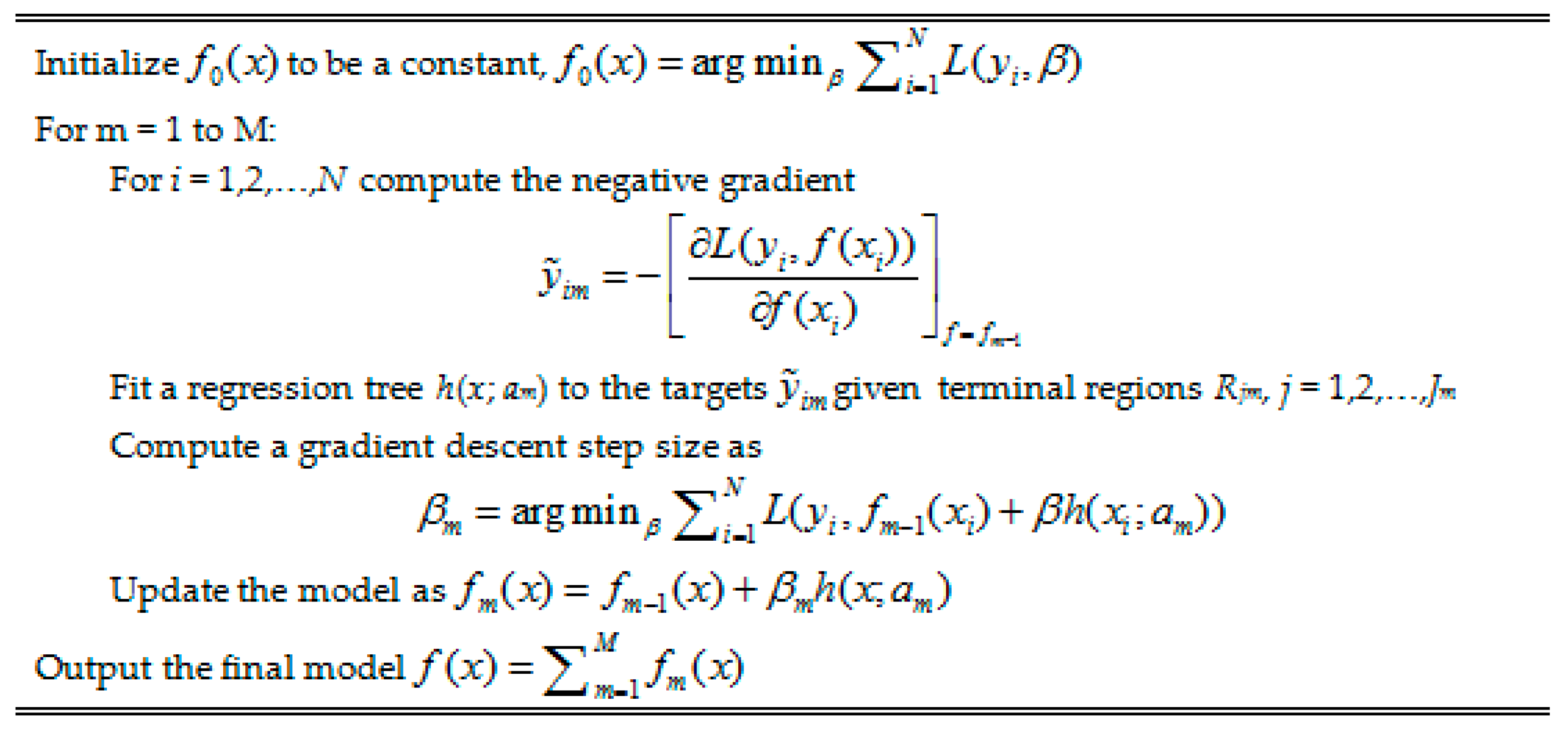
This study aims to bridge this gap by considering the access trips generated from adjacent bus stops in short-term subway ridership forecasting. A Gradient Boosting Decision Trees (GBDT) approach is proposed to capture the subtle and sudden changes of short-term subway ridership based on a series of influential factors. Different from traditional CI-based algorithms and classic statistical methods, GBDT can strategically combine several simple tree models to achieve optimized prediction performance while interpreting model results by identifying the key explanatory variables [24]. In addition, GBDT poses few restrictions and hypotheses on input data and thus is very flexible to deal with complex nonlinear relationship. These features enable GBDT to be a suitable countermeasure to predict and explain the high variability and randomness of subway passenger flows. In this study, a series of spatial and temporal factors, including historical passenger flows, time of day and transfer ridership generated by feeder buses, are incorporated into the GBDT model for short-time subway ridership. Significant relevant variables and the degree of how these variables impact future subway ridership can be identified and computed. To further demonstrate the transferability and accuracy of the proposed prediction algorithms, three subway stations with different land uses are tested to explain spatial heterogeneity. Such an approach contributes to the current literature on understanding the interaction between transfer connectivity and subway ridership forecasting in a multimodal public transit system.

The remainder of this paper is organized as follows: Section 2 describes the methodology of GBDT and documents the context of using GBDT for short-term subway ridership prediction. Section 3 presents the background of Beijing subway system with a detailed explanation of potential influential variables. Model analysis results and discussion are demonstrated in Section 4, and followed by conclusion and future research directions at the end of this paper.

2. Methodology

2.1. Gradient Boosting Decision Trees Approach

In this study, a recently developed methodological approach called gradient boosting decision trees (GBDT) was incorporated into station-level short-term subway ridership prediction. Assuming that x is a set of predictor variables and f(x) is an approximation function of the response variable y, using the training data ${\left\{y_i,x_i\right\}}_1^N$, the GBDT approach iteratively constructs M different individual decisions trees h(x; a₁),…,h(x; a_M), then f(x) could be expressed as an additive expansion of basis function h(x; a_m) as follows:

$$\{\begin{array}{l}f(x)={\displaystyle \sum _{m=1}^M{f}_m(x)}={\displaystyle \sum _{m=1}^M{\beta }_{m}h(x;a_m)}\\ h(x;a_m)={\displaystyle \sum _{j=1}^J{\gamma }_{jm}I(x\in R_{jm}),whereI=1ifx\in R_{jm}};I=0,otherwise\end{array}$$

(1)

where each tree partitions the input space into J disjoint regions R_1m, …, R_jm and predicts a constant value γ_jm for region R_jm. The parameters β_m represent weights given to the nodes of each tree in the collection and determine how predictions from the individual decision trees are combined [25,26]. The parameters a_m represents the mean values of split locations and the terminal node for each splitting variables in the individual decision tree. The parameters β_m and a_m are estimated by minimizing a specified loss function L(y, f(x)) that indicates a measure of prediction performance [27].

Defining an additive function that is combined from the first decision tree to the (m − 1)th decision tree as $f_{m-1}(x)$, the parameters β_m and a_m should be determined as follows [28]:

$$\begin{array}{ll}({\beta }_m,a_m)& =\arg \underset{\beta ,a}{\min }{\displaystyle \sum _{i=1}^{N}L(y_i,f_{m-1}(x_i)+\beta h(x_i;a))}\\ & =\arg \underset{\beta ,a}{\min }{\displaystyle \sum _{i=1}^{N}L(y_i,f_{m-1}(x_i)+\beta {\displaystyle \sum _{j=1}^J{\gamma }_j}I(x_i\in R_j))}\end{array}$$

(2)

and

$$f_m(x)=f_{m-1}(x)+{\beta }_{m}h(x;a_m)=f_{m-1}(x)+{\beta }_m{\displaystyle \sum _{j=1}^J{\gamma }_{jm}I(x\in R_{jm})}$$

(3)

Generally, it is not straightforward to solve Equation (2) due to the poor performance of squared error loss and exponential loss functions for non-robust data or censored data [29]. To overcome this problem, Friedman devised the gradient boosting approach [30], which is an approximation technique that applies the method of steepest descent to forward stagewise estimation. Gradient boosting approximation can solve the above equation for arbitrary loss functions with a two-step procedure. First, the parameters $a_m$ for the decision tree can be estimated by approximating a gradient with respect to the current function $f_{m-1}(x)$ in the sense of least square error as follows:

$$a_m=\arg \underset{a,\beta }{\min }{\displaystyle \sum _{i=1}^N{[{\tilde{y}}_{im}-\beta h(x_i;a)]}^2}=\arg \underset{a,\beta }{\min }{\displaystyle \sum _{i=1}^N{[{\tilde{y}}_{im}-\beta {\displaystyle \sum _{j=1}^J{\gamma }_{j}I(x_i\in R_j)}]}^2}$$

(4)

where ${\tilde{y}}_{im}$ is the gradient and is given by

$${\tilde{y}}_{im}=-{\left[\frac{\partial L(y_i,f(x_i))}{\partial f(x_i)}\right]}_{f(x)=f_{m-1}(x)}$$

(5)

Then, the optimal value of the parameters β_m can be determined given h(x, a_m):

$$\begin{array}{ll}{\beta }_m& =\arg \underset{\beta }{\min }{\displaystyle \sum _{i=1}^{N}L(y_i,f_{m-1}(x_i)+\beta h(x_i;a_m))}\\ & =\arg \underset{\beta }{\min }{\displaystyle \sum _{i=1}^{N}L(y_i,f_{m-1}(x_i)+\beta {\displaystyle \sum _{j=1}^J{\gamma }_{jm}I(x_i\in R_{jm})})}\end{array}$$

(6)

The gradient boosting approach replaces a potentially difficult function optimization problem in Equation (2) with the least-squares function minimization as Equation (4), and then, the calculated a_m can be introduced into Equation (6) for a single parameter optimization. Thus, for any h(x; a) for which a feasible least-squares algorithm exists, optimal solutions can be computed by solving Equations (4) and (6) via any differentiable loss function in conjunction with forward stagewise additive modeling. Based on the above discussion, the algorithm for the gradient boosting decision trees can be summarized as follows in Figure 1 [24,28,29]:

2.2. Regularization Parameters

The gradient boosting decision tree builds the model in a stagewise fashion and updates the model by minimizing the expected value of certain loss function. However, fitting the training data too closely can be counterproductive due to reducing the expected loss on the training data. When such a reduction exceeds a certain point, the population-expected loss will stop decreasing and then start increasing [28]. A regularization process can prevent such over-fitting and improve prediction accuracy by optimizing three parameters: number of trees (M), learning rate (ξ), and tree complexity (C). If the number of trees (i.e., iterations) is too small, the model cannot be fitted well. By increasing the number of trees (i.e., iterations), the model becomes complex and fits the data well. However, if the number of trees is too large, this will cause the over-fitting problem [30,31]. Learning rate, also called shrinkage, is used to scale the contribution of each base tree model by introducing a factor of ξ (0 < ξ ≤ 1) as shown in Equation (7):

$$f_m(x)=f_{m-1}(x)+\xi \times {\beta }_{m}h(x;a_m)=f_{m-1}(x)+\xi \times {\beta }_m{\displaystyle \sum _{j=1}^J{\gamma }_{jm}I(x\in R_{jm})},where0<\xi \le 1$$

(7)

where the smaller ξ is, the greater the shrinkage becomes. The over-fitting issue can be overcome by reducing or shrinking the impact of each additional tree. Smaller shrinkage values can better minimize the loss function. However, it requires a larger number of trees to be added into the model. Therefore, there is a tradeoff between the number of trees and the learning rate. Depending on the value of the learning rate and the dataset, the easiest way to find the optimal number of trees is to check how well the model fits on a validation dataset [31].

The gradient boosting algorithm also requires the specification of tree complexity. Tree complexity refers to the number of splits (or the number of nodes) that is used for fitting for each decision tree. The number of nodes equals the number of splits plus one. It represents the depth of variable interaction in a tree. Specifying one split corresponds to an additive model with only one main effect at each tree. Specifying two splits correspond to a model with two-way interactions at each tree. Generally, specifying C splits corresponds to a model with up to C-way interactions. To capture more complex interactions among variables and fully utilize the strength of gradient boosting decision trees, it is necessary to increase the tree complexity. Hastie et al. suggest that 2 ≤ C ≤ 5 generally works well [29]. Optimal performance of the model depends on selecting the combination of number of trees (M), learning rate (ξ), and tree complexity (C).

2.3. Relative Importance of Influential Factors

Generally, the influences of predictor variables on response variables are distinct, and identifying such differences is especially desirable. However, accuracy and interpretability, which are two fundamental objectives of predictive learning, do not always coincide [32]. In contrast to the statistical modeling approach and machine learning algorithms, such as autoregressive integrated moving average (ARIMA) type model, support vector machines (SVM), and neural networks, the GBDT model can identify and rank the influences of predictor variables on response predictions, while still maintaining a relative high accuracy.

For a single decision tree T, Breiman et al. proposed the following measure as an approximation of relative importance of the factor x_κ in predicting the response [33]:

$$I_{\kappa }^2(T)={\displaystyle \sum _{t=1}^{J-1}{\widehat{\tau }}_t^{2}I(v(t)=\kappa )}$$

(8)

where the summation is over the non-terminal nodes t of J-terminal node tree T, x_κ is the splitting variable associated with node t, and ${\widehat{\tau }}_t^2$ is the corresponding empirical improvement in squared error as a result of using the splitting variable x_κ as the non-terminal node t. For a collection of decision trees ${\left\{T_m\right\}}_1^M$, obtained through the gradient boosting approach, Equation (8) can be generalized by its average over all of the additive trees:

$$I_{\kappa }^2=\frac{1}{M}{\displaystyle \sum _{m=1}^M{I}_{\kappa }^2(T_m)}$$

(9)

3. Data Sources and Preparation

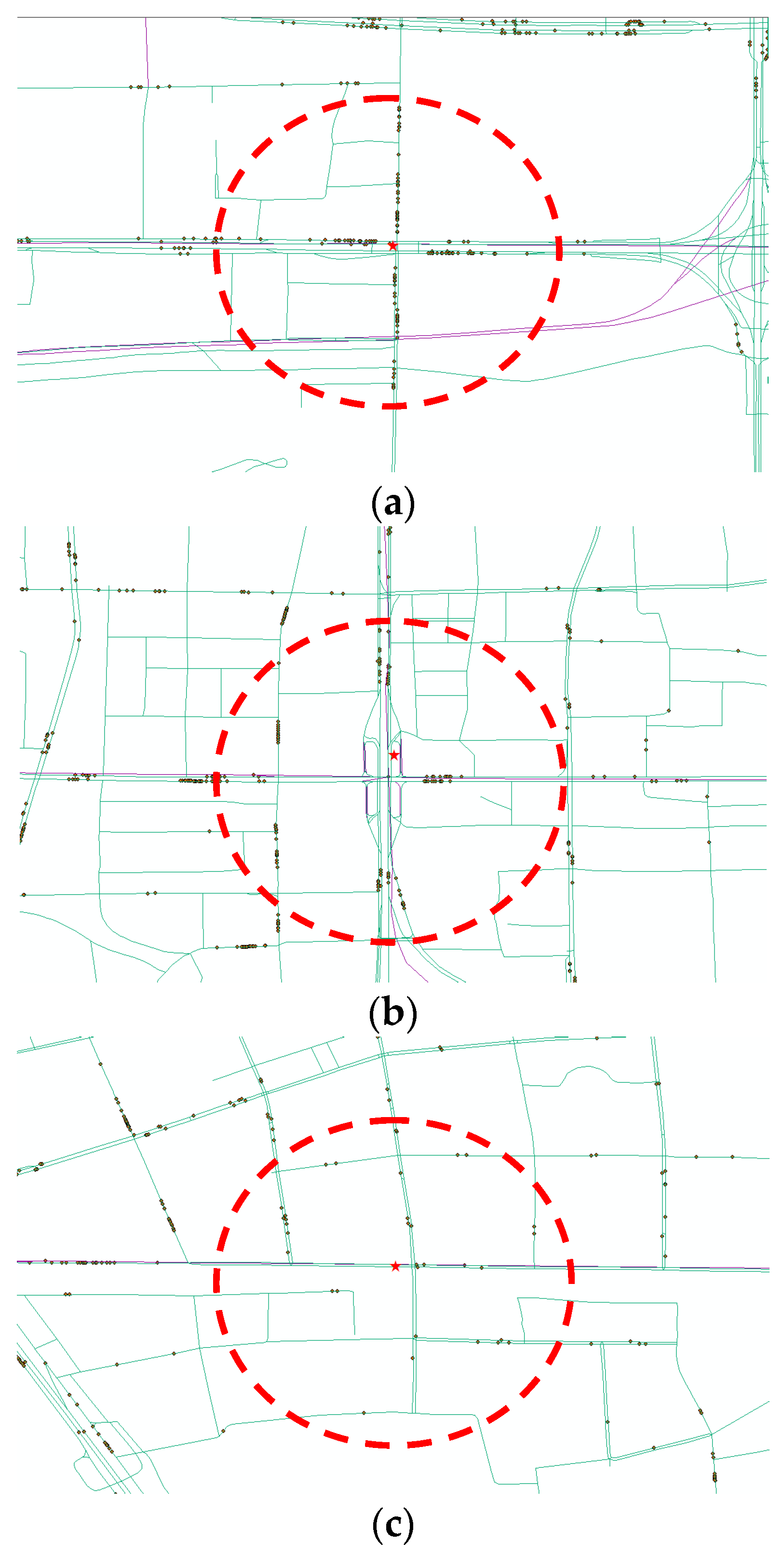
The Beijing subway network has been expanding from 4 lines with 114 km in 2006 to 16 lines with 442 km in 2012, leading to a sudden increase of daily ridership from 1.93 million to 6.74 million [34]. Such a burst of ridership stimulates several critical issues such as crowdedness in trains and insufficient capacity of transferring channels between different lines. To balance the overwhelming passenger demands and limited capacity of subway facilities, 51 subway stations began to restrict passengers’ access during certain time periods (e.g., morning and evening peak hours) in 2015. Among these stations, Da-Wang-Lu (DWL) station, Fu-Xing-Men (FXM) station and Hui-Long-Guan (HLG) station are the three most representative ones with high passenger demands in the Beijing subway system. This is owing to the surrounding land use and built environment attracting a significantly large number of passengers: The DWL station locates in the area of Central Business District (CBD) in Beijing with a wealth of Fortune 500 enterprises and shopping malls, and it also serves as a multimodal transfer hub that embraces multiple bus stops, which connects numerous commuters living in suburban to work in other districts via subway systems. The FXM station sits along the Beijing Financial Street, which is considered as one of the most significant streets in Beijing. A number of foreign and domestic financial companies and government agencies are located around the FXM station. Due to the limited parking space, the majority of commuters take the subway or bus for working in those institutions. Different from the FXM and DWL stations, the HLG station is located in a suburban residential area, where a myriad of residents live and commute to downtown on a daily basis. The layout of the three stations is presented in Figure 2, where the red pentagram indicates the target subway stations (DWL, FXM and HLG) and black dots represent the adjacent bus stops. In the field of transportation and urban planning, the 500-m circle around the subway station is generally seen as the best transit catchment [35,36]. This respectively yields 35, 26 and 15 transfer bus stops that are within passenger walking distances for DWL, FXM and HLG stations.

The acquisition of transit ridership relies on Automatic Fare Collection (AFC) techniques (also known as Smart Card). Transit smart cards have been issued in Beijing bus and subway systems since 2006 with 50% fare reduction for adults and 75% fare reduction for students. Such a substantial fare promotion quickly stimulates the wide usage of smart cards, and more than 90% passengers are smart card holders [37]. Transit fares on all routes (for bus and subway) have changed to distance-based schedules since December 2014, where passengers have to swipe their cards twice, with both boarding and alighting stops recorded. Prior to 2014, more than half of buses implemented the flat-fare strategy: Passengers are only required to tap the cards on boarding, and thus leave no alighting information for these buses. For other buses and subway systems, distance-based fare collection methods were adopted. The dataset used in this study was collected from the DWL, FXM, HLG subway stations and its adjacent bus stops between July 2012 and November 2012. The alighting stops for those flat-fare based buses can be properly inferred by using the approach proposed by [23,24], and the number of passengers transferring from buses to subway can then be estimated by counting the alighting passengers. Similarly, the subway ridership can be calculated based on the smart card transactions entering the station. Both bus ridership and subway ridership is aggregated to the interval of every 15 min. The setting of 15 min is attributed to the common practice of computing peak 15-min rate of passenger flow [38]. 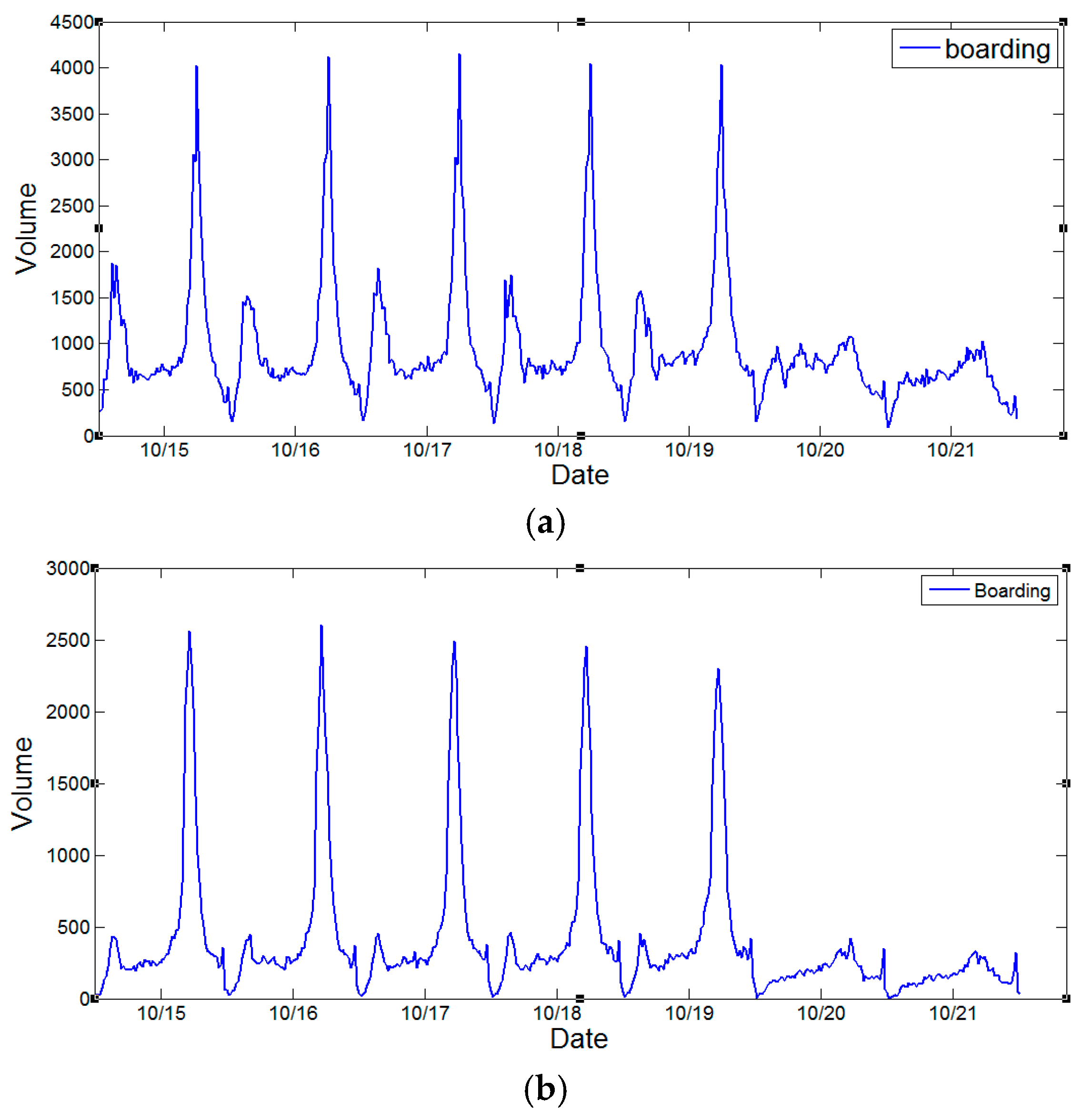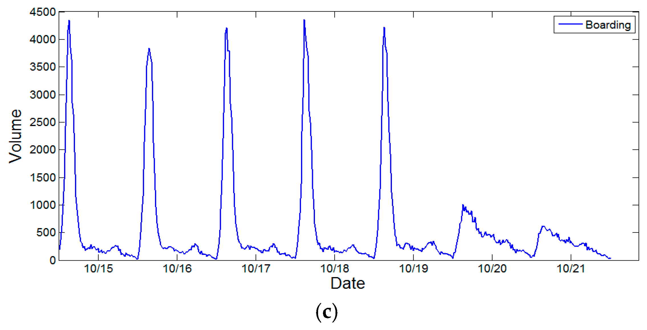Figure 3 demonstrates the weekly ridership changes at DWL, FXM and HLG stations from 15 October 2012 to 21 October 2012. For each date, the service time of subway system is from 5:00 a.m. to 11:55 p.m. The temporal distributions of subway ridership for different station vary. For DWL station, ridership exhibits a dual-peak effect since most commuters need to transfer in DWL station. For FXM station, most boarding activities occur during evening peak hours rather than morning peak hours. This is because the FXM station is adjacent to a large business and financial center, where people need to take the subway returning home in the evening. The temporal distribution of ridership in HLG station presents a reverse pattern compared with that of FXM station. The surrounding land type is residential, and thus commuters can walk to the subway station for work in the morning. However, these trends become less obvious during weekends since few people need to work on those days.

Based on the aforementioned discussion, the multimodal transfer activities are found to be strongly associated with subway ridership. Therefore, the numbers of alighting passengers at time steps t, t − 1, t − 2, t − 3 from adjacent bus stops are respectively selected as the primary independent variable with the underlying assumption of at most one-hour transfer time from buses to the subway system. Additionally, the three most relevant subway passenger demands at time steps t − 1, t − 2, t − 3 are used as inputs since the current subway ridership has strong correlations with the past ridership within one hour. Temporal factors such as time of day, day, week and month are also incorporated in the prediction model.

Table 1. Description of candidate predictor variables for short-term subway ridership.

Categories	Variables	Variable Description	Value Set
Subway station characteristics	METROt−1	Short-term subway ridership at time step t − 1	Continuous variable: R+
	METROt−2	Short-term subway ridership at time step t − 2	Continuous variable: R+
	METROt−3	Short-term subway ridership at time step t − 3	Continuous variable: R+
Bus transfer activities characteristics	BUSt	Number of bus alighting passengers at time step t	Continuous variable: R+
	BUSt−1	Number of bus alighting passengers at time step t − 1	Continuous variable: R+
	BUSt−2	Number of bus alighting passengers at time step t − 2	Continuous variable: R+
	BUSt−3	Number of bus alighting passengers at time step t − 3	Continuous variable: R+
Temporal characteristics	Time of day	Every fifteen minute time step of given day indexed from 1 to 96	Categorical variable: {1, 2, 3, …, 96}
	Date of month	Serial date number of given month that represents from 1 to 31	Categorical variable: {1, 2, 3, …, 31}
	Day of week	Serial day number of given week that represents from Monday to Sunday	Categorical variable: {1, 2, 3, …, 7}

Note: Numbers 1, 2, 3, …, 7 indicate Monday, Tuesday, Wednesday, Thursday, Friday, Saturday and Sunday, respectively.

provides the overall description of candidate predictor variables for short-term subway ridership in this study.

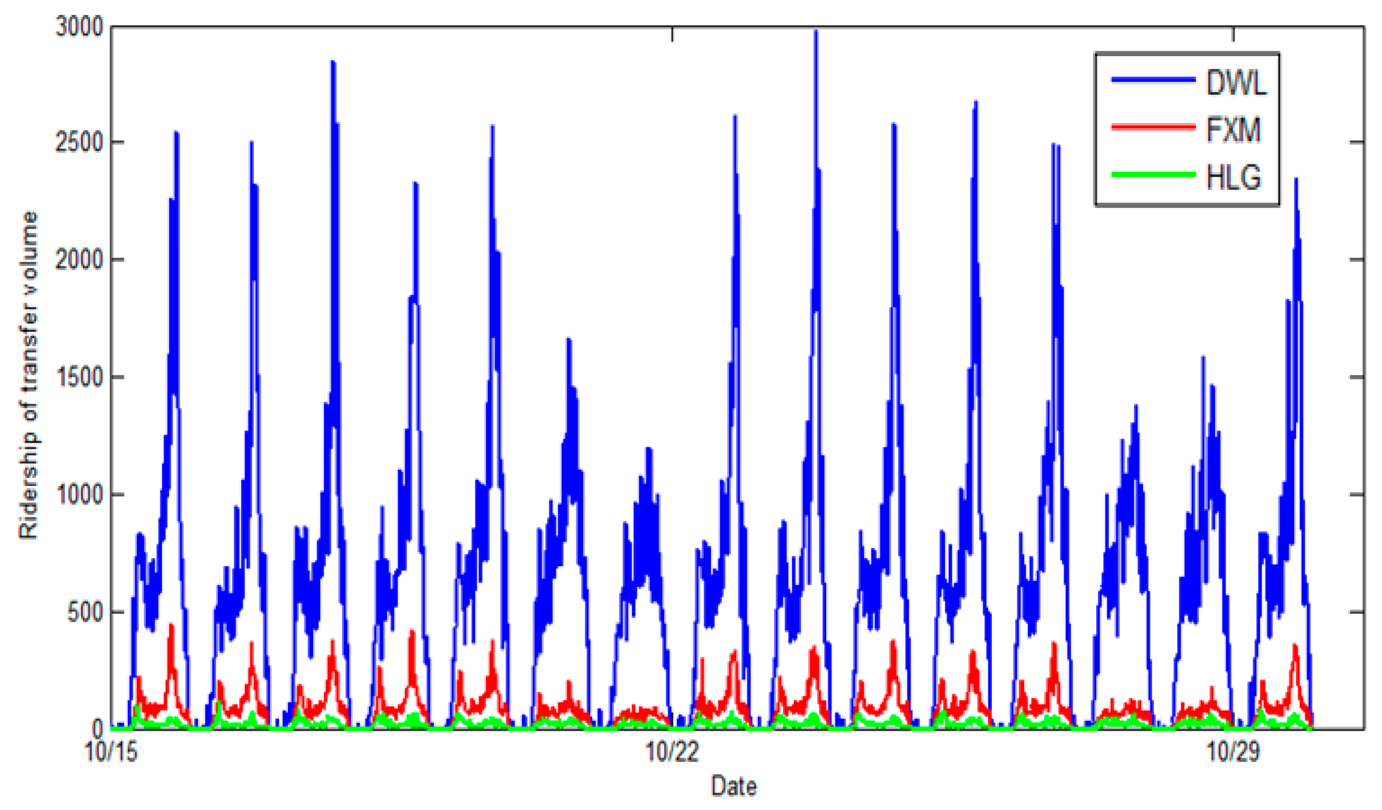
We also investigate the relationship between subway ridership and transfer passenger flows from buses. Figure 4 demonstrates the weekly ridership changes of the transfer volumes from buses at the three subway stations. The trends are consistent with Figure 3, indicating that the bus transfer activities are highly coupled with the subway ridership.

Table 2. Correlation coefficients between subway ridership and transfer volumes from buses.

Subway Ridership (METROt)	Bus Transfer Volume (BUSt−1)	Bus Transfer Volume (BUSt−2)	Bus Transfer Volume (BUSt−3)
Da-Wang-Lu (DWL)	0.243 **	0.174 **	0.044 *
Fu-Xing-Men (FXM)	0.371 **	0.277 **	0.201 **
Hui-Long-Guan (HLG)	0.311 **	0.276 **	0.226 **

Notes: ** indicates the significant correlation exists at the 0.01 level; * indicates the significant correlation exists at the 0.05 level.

computes the correlation coefficients between two variables (subway ridership and transfer volumes from buses). The level of correlation decreases as the time step increases.

4. Model Results

4.1. Model Setup

In this study, bagging is the variation used on the boosting algorithm. For the gradient boosting algorithm, only a random fraction of the residuals is selected to build the tree in each iteration. Unselected residuals are not used in that iteration at all [31]. The randomization is considered to reduce the variation of the final prediction without affecting bias. While not all observations are used in each iteration, all observations are eventually used across all iterations. Bagging with 50% of the data is generally recommended [29,30].

For the performance of short-term subway ridership modeling, the pseudo-R² is used as the measures in this study. Gradient boosting process determines the number of iterations that maximizes the likelihood or, equivalently, the pseudo-R². The pseudo-R² is defined as R² = 1 − L1/L0, where L1 and L0 are the log likelihood of the full model and intercept-only model, respectively. In the case of Gaussian (normal) regression, the pseudo-R² turns into the familiar R² that can be interpreted as “fraction of variance explained by the model” [31]. For Gaussian regression, it is sometime convenient to compute R² as follows:

$$R^2=\frac{Var(y)-MSE(y,\widehat{y})}{Var(y)}=1-\frac{{\displaystyle \sum _{i=1}^T{(f(x_i)-y_i)}^2}}{{\displaystyle \sum _{i=1}^T{(y_i-\overline{y})}^2}}$$

(10)

where $Var(y)$ and $MSE(y,\widehat{y})$ refer to the variance and mean squared error, respectively. T is the number of test samples, f(x_i) is the model prediction, and $\overline{y}$ is the mean of the test samples. In this study, the test R² is calculated on the test data based on the training model.

The data in this study is divided into three subsets: 50% of the total samples were used for model training, 25% of the total samples were used as validation dataset for model selection, and the remaining 25% were used as test dataset to assess the model performance.

4.2. Model Optimization

To validate the model performance of different combination of regularization parameters, a series of GBDT models are built with various learning rate (ξ = 0.10–0.001), tree complexity (C = 1, 2, 3, 4, 5) by fitting a maximum of M = 30,000 trees. In the gradient boosting process, the maximum number of trees is specified in this study, and the optimal number of trees that maximizes the log likelihood on a validation dataset is automatically found. Therefore, in this study the number of trees is not controlled, since an optimal solution has been achieved. For the three subway stations, the performance of GBDT models based on different combination of regularization parameters are described in the following tables. Meanwhile, given the different combination of shrinkage and tree complexity, the optimal number of trees for each model at which the minimum error is achieved is also found. In this case, if the number of trees continues to increase, then the over-fitting issues will arise.

Using the validation dataset, the influence of the shrinkage parameter on model performance can be seen in

Table 3. Performance of gradient boosting decision trees (GBDT) models for Da-Wang-Lu (DWL) subway station.

Shrinkage	R-Squared and Optimal Number of Trees
	Tree Complexity = 1		Tree Complexity = 2		Tree Complexity = 3		Tree Complexity = 4		Tree Complexity = 5
	R2	Trees	R2	Trees	R2	Trees	R2	Trees	R2	Trees
0.10	0.9565	1571	0.9742	2400	0.9764	547	0.9753	675	0.9802	429
0.05	0.9577	5730	0.9733	3383	0.9770	2894	0.9792	1617	0.9806	604
0.01	0.9605	26,851	0.9771	18,709	0.9798	14,063	0.9796	10,257	0.9807	12,479
0.005	0.9595	29,772	0.9771	29,972	0.9802	27,468	0.9803	23,201	0.9811	19,177
0.001	0.9523	30,000 *	0.9724	29,999 *	0.9776	29,999 *	0.9796	29,999 *	0.9806	29,999 *

,

Table 4. Performance of GBDT models for Fu-Xing-Men (FXM) subway station.

Shrinkage	R-Squared and Optimal Number of Trees
	Tree Complexity = 1		Tree Complexity = 2		Tree Complexity = 3		Tree Complexity = 4		Tree Complexity = 5
	R2	Trees	R2	Trees	R2	Trees	R2	Trees	R2	Trees
0.10	0.9738	10,527	0.9795	2202	0.9859	464	0.9863	602	0.9869	219
0.05	0.9759	25,516	0.9809	2107	0.9871	1570	0.9881	1013	0.9879	533
0.01	0.9756	29,997	0.9835	23,318	0.9876	10,289	0.9891	7209	0.9893	2912
0.005	0.9743	30,000 *	0.9836	29,817	0.9878	19,983	0.9890	11,473	0.9893	6743
0.001	0.9653	30,000 *	0.9819	30,000 *	0.9875	29,995	0.9888	29,982	0.9891	29,992

and

Table 5. Performance of GBDT models for Hui-Long-Guan (HLG) subway station.

Shrinkage	R-Squared and Optimal Number of Trees
	Tree Complexity = 1		Tree Complexity = 2		Tree Complexity = 3		Tree Complexity = 4		Tree Complexity = 5
	R2	Trees	R2	Trees	R2	Trees	R2	Trees	R2	Trees
0.10	0.9808	4236	0.9888	1072	0.9916	217	0.9916	457	0.9894	303
0.05	0.9827	5386	0.98884	1965	0.9905	1365	0.9905	1757	0.9910	1113
0.01	0.9835	28,242	0.9898	10,598	0.9916	7895	0.9914	5694	0.9915	5493
0.005	0.9831	29,978	0.9901	19,910	0.9915	17,596	0.9914	14,583	0.9916	8431
0.001	0.9786	30,000 *	0.9896	29984	0.9911	30,000 *	0.9915	29,927	0.9915	29,981

. For a given tree complexity, increasing the value of the shrinkage parameter will need fewer trees and less computational time to achieve its minimum error. This is due to the fact that a higher value of shrinkage parameter can increase the contribution of each tree in the model thereby needing fewer trees to be added. Depending on the tree complexity and number of trees, the optimal shrinkage parameter varies. Generally, as shrinkage parameter decreases, the model will obtain a better performance. However, when the value of shrinkage parameter reaches to a certain level, the model performance begins to deteriorate. Taking DWL subway station as an example, the model performance with C = 1 becomes better as the shrinkage parameter value decreases from ξ = 0.10 to ξ = 0.01. However, decreasing the value of shrinkage parameter from ξ = 0.01 to ξ = 0.001 leads to a worse result. To gain a better model performance, a reasonable combination of shrinkage parameter and number of trees is preferable. It should be noted that * indicates the optimal number of trees is larger than the given maximum value, and R² did not reach its best value in following tables.

The impact of tree complexity on model performance can also be quantified through Table 3, Table 4 and Table 5. For a given shrinkage parameter, increasing the value of tree complexity will generally lead to a more complex model, and thus requires fewer trees for a minimum error. Controlling the value of shrinkage parameter and number of trees, the computational time will increase as the level of tree complexity increases. Therefore, the final computational time depends on the tree complexity and optimal number of trees. Generally, the model will obtain better performance as the tree complexity increases. Taking DWL subway station as an example, the model performance becomes better with ξ = 0.10 when the tree complexity increase from C = 2 to C = 5. This is due to the fact that a higher level of tree complexity can capture more detailed information from the dataset. However, the improvement of model performance is not sensitive after the value of tree complexity reaches a certain level. Therefore, the model performance and computational time should be balanced.

Table 3, Table 4 and Table 5 present the model performances for the DWL, FXM and HLG subway stations. By comparing the model results and computational time, the best model performance for the three subway stations can be acquired, which are in bold. For the DWL subway station, the best performance is obtained at the shrinkage parameter of 0.05 and tree complexity of 5 with an optimal ensemble of 604 trees. Similar to the FXM subway station, the best model performance occurs at the shrinkage parameter of 0.01 and tree complexity of 5 with an optimal ensemble of 2912 trees. With regards to the HLG subway station, the model reached its best performance with the shrinkage parameter of 0.10, tree complexity of 3, and optimal ensemble of 217 trees. The final R² for the three optimal models are 0.9806, 0.9893 and 0.9916, respectively. This indicates a good prediction accuracy since the GBDT model is able to handle different types of predictor variables, capture interactions among the predictor variables and fit complex nonlinear relationship [39]. Hence, in this study the GBDT model can handle the nonlinear features of short-term subway ridership and leads to superior prediction accuracy. Similar studies on gradient boosting trees in travel time prediction [24] and auto insurance loss cost prediction can be also found [32].

4.3. Model Comparison

To examine the effectiveness of GBDT model used for station-level short-term subway ridership prediction, a comparison was conducted with several conventional techniques including BP-neural network, support vector machine (SVM) and random forest (RF). For BP-neural network, the learning rate is set as 0.1, and the optimal number of hidden layer neurons is calculated as 3 by using the empirical equation in [40]. For SVM, the Radial Basis Function (RBF) is selected as the kernel function. Through the three-fold cross-validation, the gamma parameter of the RBF is computed as 0.125, 1, and 0.5 for DWL, FXM and HLG stations, respectively, and the soft margin parameter C is calculated as 1. For RF, the number of tress grown is 500, and the number of predictors sampled for splitting at each node is determined as 2.

Table 6. Comparison with different models for subway ridership prediction.

Subway Station	Performance for Different Models (Measured by Root Mean Squared Error (RMSE) and R2)
	NN		SVM		RF		GBDT
	RMSE	R2	RMSE	R2	RMSE	R2	RMSE	R2
DWL	134.2033	0.9599	171.4534	0.9346	107.6754	0.9742	65.9933	0.9806
FXM	60.9258	0.9825	88.1399	0.9633	68.2797	0.9780	37.4414	0.9893
HLG	99.4166	0.9837	149.4753	0.9631	125.6164	0.9739	64.0564	0.9916

Note: NN = BP-neural network, SVM = support vector machine, and RF = random forest.

shows the comparison results for the DWL, FXM and HLG subway stations, respectively. In this study, root mean squared error (RMSE) is used additionally with R² as the model performance indicators. Lower RMSE value or higher R² value means higher accuracy. The RMSE is defined as follows:

$$RMSE=\sqrt{\frac{{\displaystyle \sum _{i=1}^T{({\widehat{y}}_i-y_i)}^2}}{N}}$$

(11)

where N is the number of test samples, ${\widehat{y}}_i$ is the predicted values, and $y_i$ is the observed values.

A statistical test is performed to evaluate the statistical significance of the results. By comparing the results of different prediction techniques, we can see that the GBDT model is statistically different to any of other techniques, and receives the best model performance for all the three stations. Overall, the GBDT model outperforms the other three models in station-level short-term subway ridership prediction in terms of both RMSE and R² measurements. As another ensemble learning method, Random Forest yields the best prediction results among other three approaches excluding GBDT with at most 36% increase of the RMSE value. On the contrary, SVM receives the worst performance for subway ridership prediction at the three stations. This finding further confirms the advantage of GBDT model in modeling complex relations between subway boarding ridership and bus transfer activities.

4.4. Model Interpretation

To explore the different influences of predictor variables on short-term subway ridership among the DWL, FXM and HLG subway stations, the relative contributions of predictor variables for the three subway stations were calculated using the optimal models as shown in Table 6, respectively. A higher value of relative importance indicates stronger influences of predictor variables in predicting short-term subway ridership.

As shown in

Table 7. Relative influence of predictor variables on short-term subway ridership.

Variable	DWL Subway Station		FXM Subway Station		HLG Subway Station
	Rank	Relative Importance (%)	Rank	Relative Importance (%)	Rank	Relative Importance (%)
METROt−1	1	82.03	1	85.06	1	92.28
METROt−2	4	1.71	4	0.95	4	0.20
METROt−3	5	1.65	5	0.77	3	0.46
BUSt	2	9.41	3	4.42	8	0.08
BUSt−1	6	0.55	6	0.44	6	0.11
BUSt−2	8	0.40	7	0.34	9	0.06
BUSt−3	7	0.41	8	0.27	5	0.16
Time of day	3	3.55	2	7.59	2	6.54
Date of month	10	0.12	9	0.10	7	0.10
Day of week	9	0.17	10	0.06	10	0.01

, each predictor variable has a different impact on short-term subway ridership. For all the three subway stations, the immediate previous subway ridership METRO_t−1 contributes most in predicting short-term subway ridership with a relative importance of 82.03%, 85.06% and 92.28% for the three subway stations, respectively. This finding falls within our expectation that the immediate previous ridership is closely related with the current subway ridership. The current bus alighting passengers BUS_t, with a contribution of 9.41%, 4.42% and 0.08% to the short-term subway ridership prediction, respectively ranks the second, third and eighth most influential predictor variable for the DWL, FXM and HLG subway stations. This result indicates that the bus transfer activities around the DWL subway station have the most potentially significant effects on the subway ridership, and the bus transfer activities around the HLG subway station have little effects on the subway ridership. This is consistent with the fact that the DWL subway station is an important transfer station, and a number of residents live around the HLG subway without needing transfer. For FXM station, bus transfer activities contribute less than 5% of ridership. This is because the station is actually within walking distance of Beijing Finance Street, where office workers can directly take subway for commuting. Meanwhile, 26 bus stops are around FXM station, and these stops still transfer a certain amount of passengers to the subway system.

Another interesting finding relates to the influence of time of day on short-term subway ridership. For the three subway stations, the influence of time of day contributes 3.55%, 7.59% and 6.54% to the short-term subway ridership, respectively. The factor of time of day is associated with the periodic feature of subway ridership: subway ridership is usually high during peak hours and maintains at a moderate level of ridership during non-peak hours. This finding confirmed the important role of time of day in predicting subway ridership. Among other variables, the short-term subway ridership at time step t − 2 METRO_t−2 and at time step t − 3 METRO_t−3 have slightly over 1% of contributions in predicting subway ridership for the DWL subway station, while their contributions become less than 1% for the FXM and HLG subway stations.

5. Summary and Discussion

Public Transportation plays an important role in reducing fuel consumption, lowering vehicle emissions and alleviating traffic congestion. As reported in Park and Lee’s study, a strong positive relationship between bus ridership and airborne particulate matter (PM10) can be found [41]. Therefore, maximizing transit ridership will ultimately improve air quality. This study ranks the potential influential factors on subway ridership, and investigates how varying the built environment impacts on passenger transfer activities to subway systems. The research outcomes provide useful information to design and optimize public transit facilities for attracting more passengers from private cars to the public transport mode, and are expected to enhance the sustainability of the transportation system.

This study contributes to improving short-term subway ridership prediction, accounting for bus transfer activities in a multimodal public transit system. The GBDT model is proposed to handle different types of predictor variables, fit complex nonlinear relationships, and automatically disentangle interaction effects between influential factors. Three subway stations with different land uses are selected to explain the spatial heterogeneity. For each station, the short-term subway ridership and bus alighting passengers are obtained based on the transit smart card data. Moreover, a series of temporal factors are incorporated into the GBDT model for short-time subway ridership. The models were built with various learning rates and tree complexities by fitting a maximum of trees.

In this study, the optimal GBDT model for each station was found by balancing algorithm effectiveness and efficiency. Our study showed that the GBDT model has superior performance in terms of prediction accuracy and model interpretation power. This is different from the traditional computational intelligence algorithms (e.g., SVM, neural networks, and random forest)—“black-box” procedures—and the relative influences of predictor variables on short-term subway ridership predictions can be identified based on the optimal GBDT model. It is greatly helpful to better understand the contribution of bus transfer activities and temporal factors on subway ridership prediction. For all three stations, the immediate previous subway ridership and time of day were found to generate the most important influence on short-term subway ridership prediction. The relative influences of bus transfer activity variables on short-term subway ridership were shown to be different according to various land uses associated with subway stations. For example, the bus transfer activities around the DWL subway station were found to yield more influences on short-term subway ridership than HLG station. These examples show that the GBDT model has the advantage of incorporating different types of predictor variables, capturing complex nonlinear relationship, and providing the relative importance of influential factors. Therefore, the GBDT model can also be applied in the field of travel time prediction, travel flow prediction, etc.

The proposed short-term subway ridership forecasting method can be applied to quantify the impact of subway ridership burst under special events. Large events (e.g., concerts or soccer games) lead to non-habitual passenger demands and may exceed the designed capacity of subway system. If the contribution of buses on subway ridership is identified, more rational and timely management strategies can be then be adopted, such as real-time train timetable adjustment and demand-driven feeder bus allocation. This is especially useful for both operators and travelers to avoid overcrowding. Meanwhile, forecasting subway ridership in the context of bus transfer activities provides insightful evidences for subway system planning. Instead of focusing on the absolute ridership during peak hours, the attractiveness to other transportation modes should be also taken into account for subway station design. One limitation of the GBDT model in this study that should be noted is that the statistical significance for influential factors cannot be captured. Further studies can be made to extend the use of the advanced GBDT model for discrete response variables such as travel model choice.