1. Introduction
Over recent years, sustainability of urban environments has become one of the key challenges of our time and a remarkable upsurge of concern about it can be observed through scientific and non-scientific literature. Considerable efforts have been invested in several methodological challenges that range from trying to define sustainable development itself [
1,
2,
3] to designing indicators that can be used to monitor it [
4,
5,
6]. Many literature sources refer to sustainable development indicators at national levels [
7,
8], while only a few take a deeper look at the city level [
9,
10], and although they all recognize the role of sustainable mobility, this topic is mainly partially covered [
9,
11] over the dispersed contexts and approaches, while holistic and systematic overview is still missing.
The aim of this paper, based on research at Ghent University commissioned by World Business Council for Sustainable Development (WBCSD), and co-creation and the reviews by expert groups and panels working within the framework of the development of SMP2.0 toolbox of the WBCSD, is to give systematic literature review of sustainable mobility indicators at urban environment level. To do this, besides the three sustainable development pillars (g—global environment, q—quality of life and e—economic success), we have added m—mobility system performance to create four dimensional space across which indicators are positioned. In addition, when reviewing sustainable mobility indicators across literature, we were guided by the principles of neutrality and transferability, meaning that when facing different indicators addressing the same issue, we tried to highlight those that are technologically neutral (meaning that they do not favour nor disfavour upcoming or existing, traditional, technological solutions), transportation mode neutral (that they do not favour nor disfavour between transportation modes) and economic development neutral (they have the same level of applicability across cities in different stages of economic development). In this way we aimed at summarizing sustainable mobility indicators across literature to a set that can be applicable and replicable in different cultural and socio-economic contexts, facilitating the transferability and scaling up of successful sustainable mobility measures and policies worldwide. In addition, when applicable, the highlighted indicators are translated into relative measures (to avoid the impact of city size on the final results) and rated on the zero to ten scales (to ensure uniformity). Special attention has been given to the input data availability, so that indicators with freely available and reliable input data (e.g., from statistical databases) are preferred, as they do not require additional funds for data collection. This was done to support equal opportunity for research groups, city’s authorities and industries worldwide in applying the highlighted indicator set. In addition, a hierarchic literature review process followed, meaning that, for each indicator topic, firstly documentation of worldwide organizations (e.g., United Nations) was reviewed, then region-wide organizations (e.g., European Commission, Asian Development Bank) documentation, then recent research project results and scientific papers. This was done to ensure full literature coverage, but also to provide a holistic overview of sustainable mobility indicators.
In the following sections, we first describe the concepts of sustainability and sustainable mobility, which provide the conceptual framework for the selection of indicators for sustainable (urban) mobility (
Section 2). In
Section 3, a measure is selected for each individual indicator. This happens in two steps: first, the frequently applied measures in literature are summarized, from which a preferable measure is selected by means of a SMART (Specific, Measurable, Achievable, Relevant, Timely) evaluation.
Section 4 concludes by describing the further application of these measures within a global evaluation methodology for sustainable urban mobility.
2. Dimensions and Indicators of Sustainable Urban Mobility
WBCSD formulates the process of developing urban sustainable mobility as follows: “The ultimate goal is to accelerate and extend access to safe, reliable and comfortable mobility for all whilst having zero traffic accidents, low environmental impacts, affordability, and reduced demands on energy and time. The movement of people and goods would be facilitated, contributing to a more prosperous and resilient society by creating new values and businesses, and a positive environmental and economic growth cycle”. To formulate sustainable mobility indicators that measure potential solutions to enable cities to better implement sustainable mobility solutions makes part of that ambition” [
12].
The ambition formulated by WBCSD reflects a holistic and dynamic approach of urban sustainable mobility, widespread in academic literature [
13,
14].
The most cited and authoritative author is David Banister. In his key article “The sustainable mobility paradigm”, he argues that “policy measures are available to improve urban sustainability in transport terms but that the main challenges relate to the necessary conditions for change. These conditions are dependent upon high-quality implementation of innovative schemes…” [
13]. He develops the contrast between conventional transport planning and the sustainable mobility approach.
Some crucial differences are that the conventional planning focuses on physical dimensions (infrastructure) in terms of mobility and the resulting (car) traffic, while a sustainable mobility approach primarily considers social dimensions, in terms of accessibility and people, either in/on a vehicle or on foot. The accessibility is not only relevant for the transportation system, but even so impacts land use, where compactness and functional diversity contribute in creating accessibility. This has impacts on several aspects of transport planning. One can say that conventional planning considers a street as a “road”, while a more sustainable approach considers it as a street. In these terms, conventional planning strives to minimize travel time and thus to speed up traffic, whereas sustainable mobility attempts to realize reasonable and reliable travel times which may require slowing down movement. For the evaluation of the transportation system, conventional planning results in an economic evaluation in terms of flows and delays. The sustainable mobility approach prefers a broader Multi-Criteria Analysis to take into account also environmental and social concerns [
13].
Based on the sustainable mobility approach described by D. Banister, the proposed indicator set was structured around four dimensions. The first three are according to the wide-spread TBL (Triple Bottom Line) concept [
15], which focuses sustainable development on the harmony between people, planet and profit (or prosperity [
16]), namely:
Global environment (g)—though the impact of urban mobility on global environment exceeds the city limits, cities have moral and in many cases binding obligations (e.g., environmental conventions) to limit the global impacts;
Economic success (e)—refers to the contribution of mobility to the welfare of the city;
Quality of life (q)—refers to the impacts of mobility on the social aspects of city life, including safety and health.
The performance of the mobility system (
m) itself is added as a fourth dimension. This fourth dimension aims to obtain a holistic approach, starting from the performance of the mobility, described in a comprehensive and systemic way: the mobility system consisting of three markets or arenas in which mobility decisions can be situated [
17].
The “mobility system” includes freight as well as persons being moved or moving around in the city area. It includes all modes relevant for city traffic (motorised and non-motorised, public as well as private modes): inland ships and boats, helicopters, trains, light trains and metro (underground), trams and busses, different types of cars, motorbikes and mopeds, bikes (e-bikes as well as regular bikes), and last but not least, walking. It includes also all levels of decisions to be taken by individuals and organisations including businesses “demanding” mobility as well as by actors offering mobility (city government, public and private organisations offering mobility services).
In the conceptual model, representing the interactions within the mobility system approach represented in scheme (
Figure 1), three levels of mobility performance are distinguished:
- -
Travel: refers to the need and the ability to move around in the city to participate in an activity (such as shopping), to provide the goods to make the functioning of the activity possible and to move the products of an activity towards other places.
- -
Transport refers to the transfer of goods and people from one place to another. Transport is performed via different transport modes, modes referring to different forms or organisation (e.g., public versus private), different types of infrastructure (road, rail, waterways and air transport) or different types of vehicles (car, train, tram, moped, bike, etc.).
- -
The transport of goods and people requires vehicles and infrastructure. The word traffic is used to describe the actual movement of vehicles across the infrastructure (or the parking of vehicles on dedicated infrastructure).
The differentiation between travel, transport and traffic is not only relevant for academic research: it refers to different “markets” (or arenas) in which different types of actors are confronted with certain types of demand and supply decisions within the mobility field. A complexity is that these three markets are interrelated (
Figure 1), meaning that certain mobility solutions offered by the transport business within one of these markets might affect—intentionally or unintentionally—the performance in the other markets.
Figure 1.
Indicators of mobility (from [
18]).
Figure 1.
Indicators of mobility (from [
18]).
For each of these dimensions, literature research was done, in order to define a set of indicators, covering all relevant aspects, as illustrated in
Figure 1. This resulted in a list of 22 indicators (
Table 1).
Table 1.
The list of 22 sustainable mobility indicators.
Table 1.
The list of 22 sustainable mobility indicators.
| Indicators for the Sustainability of Urban Mobility | Short Name | Dimension |
|---|
| Emissions of greenhouse gases | GHG | Global environment |
| Energy efficiency | Energy efficiency | Global environment |
| Net public finance | Public finance | Economic success |
| Congestion and delays | Congestion | Economic success |
| Economic opportunity | Economic opportunity | Economic success |
| Commuting travel time | Travel time | Economic success |
| Mobility space usage | Space usage | Quality of life |
| Quality of public area | Public area | Quality of life |
| Access to mobility services | Access | Quality of life |
| Traffic safety | Safety | Quality of life |
| Noise hindrance | Noise hindrance | Quality of life |
| Air polluting emissions | Air pollution | Quality of life |
| Comfort and pleasure | Comfort and pleasure | Quality of life |
| Accessibility for mobility impaired groups | Accessibility for the impaired | Mobility system performance |
| Affordability of public transport for poorest group | Affordability | Mobility system performance |
| Security | Security | Mobility system performance |
| Functional diversity | Functional diversity | Mobility system performance |
| Intermodal connectivity | Intermodal connectivity | Mobility system performance |
| Intermodal integration | Intermodal integration | Mobility system performance |
| Resilience for disaster and ecologic/social disruptions | Resilience | Mobility system performance |
| Occupancy rate | Occupancy rate | Mobility system performance |
| Opportunity for active mobility | Active mobility | Mobility system performance |
The result is a set of indicators which combines “classic” criteria, such as greenhouse gas emissions or noise hindrance, with more innovative criteria, such as affordability of public transport or accessibility for deficiency groups. This needs to result in a more integrated approach of evaluating urban mobility, enabling the evaluation of the current mobility system, but also allowing the assessment of possible actions towards more sustainable mobility.
3. Methodology for the 22 Indicators
After the selection of the indicators, a methodology needs to be defined for the evaluation of each indicator in an objective and quantified way. Therefore, the SMART methodology was selected, as it requires that the selected indicator set needs to be:
Specific, evaluating exactly the mobility aspects which are relevant for sustainable mobility;
complete (covering the whole range of sustainable mobility, including all relevant types of mobility users, transport modes, mobility impacts, etc.);
Measurable with sufficient accurateness, based on Attainable data, i.e., on existing data or easily collectable data (in order to create a methodology which is applicable for cities of varying size, region or development),
have the capability (sensitivity) of detecting relevant changes in sustainability (either ongoing progress, either due to specific projects), both positive and negative, in a time-based way (allowing a frequent update in order to monitor evolution);
technology neutral, i.e., not excluding or monopolizing specific type(s) of solution;
scalable, i.e., indicator evaluation must be independent from city size. Therefore, most indicators are related (population, geographical area, etc.).
Another methodologic limitation is that air transport and shipping are excluded from the methodology, as in most cities (the sustainability impacts of) these modes are beyond the scope of urban governance.
In the following paragraphs, the 22 indicators are outlined, subsequently giving an overview of measures applied in the current practice as found in literature, before evaluating and selecting the most suitable indicator in view of sustainable urban mobility.
3.1. Emissions of Greenhouse Gases
3.1.1. Overview of Applied Measures
The intention of this indicator is to evaluate the total emissions of greenhouse gases by all passenger and freight city transport modes, and several types of measurements for this can be found in literature. The obvious one would be to measure the total emission of greenhouse gases by the whole city’s mobility system for a given period (e.g., per day or year) and while some sources only consider the emission of CO
2 [
19,
20,
21], others advise to take the variety of greenhouse gases into account [
22]. The greenhouse gases include several types of gases with different climate impacts and most often each of them is converted into CO
2 equivalents, according to the Global Warming Potential (GWP) [
23]. The GWP describes the cumulative effect of a gas over a time horizon (usually 100 years) compared to that of CO
2, and due to the global impact of greenhouse gases, usually the total well-to-wheel production of CO
2 is considered [
23].
The main objection to measuring the total emission of greenhouse gases is that this would not meet the requirement of being scalable, as larger cities would have higher total emissions than smaller ones. Therefore, the emission of greenhouse gases needs to be scaled and is often expressed in relation to the size of the population, as either amount of CO
2 per capita [
20,
24,
25] or CO
2-equivalents per capita [
21,
26,
27,
28], or per unit of GDP [
23].
3.1.2. Selected Measure
As mentioned above, the absolute total of greenhouse gas emissions is not comparable between cities of different size, so one of the scaled measures is needed. Relating to the GDP of the city is not relevant when considering urban mobility, as it would only consider the economic value of mobility, omitting e.g., the social importance of mobility. Relating emissions to the population considered is more relevant, as the purpose is to fulfil the population’s mobility needs with the smallest impact possible. Finally, it is preferable to include all types of greenhouse gases in the evaluation by converting each type to CO2-equivalents.
This leaves the total annual well-to-wheel emission of CO2-equivalents per capita by urban transport as the best measure for this indicator. This measure can be calculated by a summation of the emission of greenhouse gases, converted to CO2-equivalents, over the different transport modes and vehicles brands for different fuel types.
3.2. Net Public Finance
3.2.1. Overview of Applied Measures
This indicator expresses to which extent the urban mobility system is financially sustainable, by comparing the net result revenues and expenditures related to city transport.
A remark to start with is that in definitions of net public finance, sometimes there is a thin line between revenues and expenditures of the transport system and the transport sector. For example, European project REFIT [
29] defines the share of the Gross Value Added generated by transport as a possible measure, indicating the direct contribution of the transport sector to national economy, where transport includes all activities related directly and indirectly to the use of vehicles, vessels and aircraft and of related infrastructures (highways, inland waterways, railways, pipelines, port facilities, airports, warehouses,
etc.) for the movement of goods and passengers. There is a need to clearly define the “mobility system” to be considered. Parameters, such as the total employment in the transport sector [
29] are relevant for the transport sector, but not for the urban mobility system. Government revenues from transport related taxes and charges, net of transport related subsidies are uniform units for the net public finance, but needs scaling in order to be comparable between cities [
29,
30]. This can be attained by expressing the net public finance related to the Gross Domestic Product (GDP). Other measures for the economic impacts of transport investments are the return on investment (ROI) or payback time [
31,
32].
3.2.2. Selected Measure
The net public finance is directly measurable as the net result of the government’s and other public authorities’ revenues from transport related taxes and charges minus investment, operational and other costs, per unit of GDP.
3.3. Congestion and Delays
3.3.1. Overview of Applied Measures
This indicator calculates the impact of congestion and delays in the urban mobility system. Literature mentions congestion as one of the most important goals for improving the sustainability of mobility [
33,
34,
35,
36] and different ways to measure this impact, from different points of view. Measures from the user’s perspective consider the size and impact of delays (e.g., time lost in congestion), while other methods measure the extent of congestion, either in time (during which period of the day does congestion occur) or in space (which part of the network suffers from congestion). Finally, a more complex indicator combines these time-related and spatial indicators.
The first class of measures focuses on people’s exposure to congestion and delays, and thus on the time lost in congestion:
The total annual amount of time lost is an intuitive measure, but needs scaling in order to be comparable between cities of different sizes, e.g., in terms of time lost in traffic congestion per capita, per road user or per road kilometre [
37] or per auto commuter [
38].
Average commute travel time partially reflects congestion and delays [
37], but is not specific as a higher commute time may have others causes (e.g., different spatial structure, with longer commute distances). Therefore, this measure overlaps with other indicators like “functional diversity” and “commute travel time”.
The ratio between peak period travel times and off-peak travel times is a very direct measure for congestion impact, although definitions differ. Some (“travel time rate”) only incorporate reoccurring delays (normal congestion delays), while other (“travel time index”) also take into account incident delays (e.g., traffic crashes) [
37,
38,
39].
Travel time reliability is expressed as the ratio between the mean travel time and its standard deviation [
40].
Other measures focus on the time dimension of congestion. These measure the period (percentage of the day) during which congestion occurs. A derived measure is the percentage of peak period travel (per vehicle or per person) which occurs under congested conditions, the “Travel time in Congestion Index” [
37].
Yet, another perspective is the network level, indicating which proportion of the road network is affected by traffic congestion.
A drawback of the above measures is that some need a uniform definition of “congestion” (e.g., in terms of speed reduction) or of a “peak period”. Also, most of the above measures cover only certain aspects of the congestion problem. Ideally, a congestion measure should incorporate the congestion level, the time period and the network extent of traffic congestion. This has led to more complex indicators, considering which part of the urban road network suffers from which level of congestion during which part of the day. As calculations are based on (big) traffic data, methodologies have been developed and applied by major companies in this field, leading to the INRIX index [
41], the TomTom Congestion Index [
42] or the IBM Commuter Pain Index [
43]. IBM Commuter Index aims at covering all types of “pain” felt by commuters, which includes congestion but even so pollution, road condition,
etc. It is therefore much broader than traffic congestion and thus not specific for this single indicator. A last consideration is that most indicators are applicable to public transport as well as to car traffic. For public transport, delays can be defined as the average distance between the average actual travel time and the scheduled travel time [
44].
3.3.2. Selected Measure
The yearly delay per car commuter is a direct reflection of the congestion impact, which is attainable based on floating car data or traffic model results. However, it does not incorporate during which share of the day period or in which portion of the road network traffic congestion occurs.
As stated above, a congestion measure should incorporate the congestion level, the time period and the network extent of traffic congestion. This requires the more complex methods, from which INRIX index and Tom Tom Congestion Index are more specific. For this reason, the application of a similar approach is most suitable for evaluating congestion and delays for car traffic. For public transport, a similar methodology should be applied by comparing actual travel time with the scheduled times.
3.4. Economic Opportunity
3.4.1. Overview of Applied Measures
This indicator intends to quantify the direct economic contribution from the city transport sector to the welfare of the metropolitan area. Obvious ways of measuring this are the share of employment in the transport sector (%) [
30,
45], the share of the population which is employed in the transport sector [
46], the percentage of the Gross Domestic Product (GDP) [
45,
46] or the Gross Value Added (GVA) [
47], which is created by the transport sector. The Transport Service output Index (TSI) is a more specific measure of the volume of services performed by the for-hire freight transportation sector [
47], and therefore covers only a part of the transport sector.
A more specific definition uses the public revenues from taxes and traffic system charging as the measure [
30], but this covers only the public part of the transport sector. Therefore, this measure is more relevant for the indicator on the net public finance of the mobility system.
The Location Quotient (LQ) calculates the relative strength of an economic sector X in a metropolitan area, compared to the national situation, as the ratio between the share of employment (employment in sector X/total employment) for the metropolitan area and the national share [
46].
3.4.2. Selected Measure
The main considerations for the selection of a measure are the attainability (availability of—uniform—base data) and specificity (representing the complete transport sector) of the measure. For these reasons, the share of the Gross Value Added (GVA) to the city transport and storage sector is chosen as the measure for economic opportunity.
3.5. Commuting Travel Time
3.5.1. Overview of Applied Measures
Commuting travel time is recognized as an important sustainable mobility indicator across the literature [
35,
48,
49,
50], mainly as an economic aspect of sustainable mobility [
51,
52] but also as a part of accessibility analysis and the role of public transport in a more sustainable modal shift [
53]. This indicator evaluates the time needed to commute from home to work or to an educational establishment (for students).
The obvious measure for this indicator is the average commuting travel time [
9,
54]. This measure should include the total door-to-door travel time, which means that travel time by car should include normal delays and time needed for parking, while travel time by public transport should include the travel time from one’s origin to a transit stop, waiting time for a transit vehicle, travel time on-board, time required for transfers during the trip and travel time from a transit stop to one’s destination [
55,
56].
A derived measure is the average travel time per 10 km journey [
57]. This excludes the effect of trip length, and puts the focus on the average commuting speed and thus on the performance of the mobility system. Another way of expressing (the perception of) the commuting travel time is monetarized value of the commuting travel time [
58]. This conversion is done by means of the Value of Travel Time (VTT), referring to the cost of time spent on transport, including waiting as well as actual travel time. VTT includes costs to consumers of personal (unpaid) time spent on travel, and costs to businesses of paid employee time spent in travel. Research on VTT has differentiated values to reflect the impact of qualitative factors such as comfort, convenience and reliability. Using these corrections, the monetarization gives a heavier weight to waiting time or travel time spent in congestion, or a lower weight to travel time used efficiently (e.g., reading or calling). The Travel Time Index is the ratio of the average peak hour travel times to the average free flow travel times [
59]. This however is more a measure for the delays during the peak periods than for the total travel time. The same goes for Travel Time Predictability (the difference between the expected and the actual travel times) and the Travel Time Variability (the measured variance in actual travel times) [
60]. A last possible measure is the percentage of commute journeys that are within a certain range of the mean commuting travel time [
61], but this again is more a measure for reliability than for the actual travel time.
3.5.2. Selected Measure
The indicator for commuting travel time is closely related to other indicators, such as congestion and delays and access to the mobility system. Therefore, the chosen measure should specifically represent the total travel time, and not the uncertainty (reliability) of the travel time. The most basic, and yet most relevant, indicator is the average actual commuting travel time. It can be collected from several sources (travel survey, floating car data) and has the lowest risk of overlaps with the indicator for congestion and delays. Note that the measure should include travel time for commuters of all available transport modes.
3.6. Mobility Space Usage
3.6.1. Overview of Applied Measures
This indicator represents the proportion of land use, taken by all city transport modes, including direct (e.g., roads, rails) and indirect uses (e.g., parking space).
A very direct measure is the total surface of the road network (and other modes), but this measure depends strongly on the size of the city and needs to be scaled, which is possible by converting it into the road surface per capita [
62], or into the share of the total area which is occupied by mobility infrastructure [
29,
63,
64]. Another way of scaling, which differentiates between modes, is relating the space use to the amount of users per mode (square metre per user) [
65]. Alternatively, the size of the network can be expressed by the total length of the road network, resulting in similar measures like the network density (road length or road surface per square kilometre) [
66] or the road length per capita [
67].
A more complex method also takes into account the time dimension, multiplying the surface taken by the time it is used (expressed in square metre hours) [
68]. This allows a logic integration of direct and indirect costs for different modes. For example, for car commuting, 8 h of vehicle parking is included, while no parking is needed in case of walking or public transport [
69].
3.6.2. Selected Measure
In order to have a complete overview of this indicator, the selected measure should include all modes, and should cover both direct and indirect costs. Indicators limited to car traffic (road network) are therefore unsuitable. Measures including the time usage of the surface are interesting, but need detailed and specific input data, which requires additional data collection (surveying). Therefore, the selected measure calculates the amount of square metre of direct and indirect mobility space usage per capita.
3.7. Quality of Public Area
3.7.1. Overview of Applied Measures
The quality of the public area describes the presence of streets and squares in the city that offer opportunities for individual contact and social interaction, and that have a good image. It is clear that this quality covers a wide range of aspects, which all have separate measures of quality.
A recurring aspect is the presence of green in the city, expressed as the percentage of green space (public parks) in relation to the city area, or in relation to the population (green area per capita) [
70]. A critique is that this measure only accounts for the size of the green areas, but not their quality. This is covered in the Green, Public space and heritage Indicator (GPI) [
71], which calculates the percentage of the green or public spaces and local heritage in need of improvement. Another important aspect is the presence of facilities for walkability, such as pedestrian areas, traffic-calmed areas, car-free paths, dropped curbs and disabled facilities, and children- and pedestrian-friendly design of public spaces [
72]. However, these measures have already been taken into account for the indicator about opportunities for active modes. Finally, also the quality of the roads is a part of the quality of public areas, quantified as the percentage of roadways which are in good condition [
70]. However, this indicator is not relevant (and even counterproductive) for the purpose of this indicator, the opportunities for social interaction in public spaces. Even so, this indicator is closely related to the indicator for space usage for mobility facilities.
As all above measures concern only certain aspects of the quality of public space, there still is a need for an indicator which evaluates the quality as a whole. This can be realized by means of the reported social usage of streets and squares, and the subjective appreciation of the quality of public area [
73].
3.7.2. Selected Measure
Most measures do not meet the requirement of being a specific measure for this indicator, as only partial aspects are measured. Therefore, the selected measure is the reported satisfaction about the quality of the public space in the city in a satisfaction survey among the population.
3.8. Access to Mobility Services
3.8.1. Overview of Applied Measures
This indicator shows whether people have sufficient access to the urban mobility services, in order to fulfill their travel needs.
A first type of measures evaluates the access to specific modes. For cars, this can be expressed by the percentage of people that have a private motor vehicle available for their use [
74,
75]. For public transport, a logical indicator is the percentage of the city’s population living within a certain range of a public transport stop. This range may be expressed as a straight distance from the stop or as walking time from the stop [
76]. Also, park-and-ride lots can be included in a similar definition. The ranges used in various sources are similar, e.g., a range of 400 m is used in [
46,
77]. The PTALs (Public Transport Accessibility Levels) method applies a maximum walking time of 8 min or a maximum walking distance of 640 m for buses, while rail and light rail services allow a maximum walking time of 12 min and a maximum walking distance of 960 m [
78]. A second approach is to measure the accessibility of specific destinations, for example expressed by the percentage of the employment within a certain range (e.g., 0.4 miles) of a transit stop [
74]. Similarly, [
79] defines employment accessibility as the number of job opportunities and commercial services within a 30-min travel distance of residents.
Transport for London’s PTALs method [
78] combines these approaches by evaluating the accessibility of specific destinations by public transport. It includes:
Walking times from specified point(s) of interest to all public transport access points (bus stops, rail stations, light rail stations, underground stations and Tramlink halts) within pre-defined catchments.
A measure of service frequency by calculating an average waiting time based on the frequency of services at each public transport access point.
A reliability factor of the public transport services.
Haase [
80] describes a similar model-based evaluation method for public transport taking into account the accessibility of key services (such as hospitals, schools, retailing, financial services,
etc.) by public transport, resulting in the Transport Accessibility Index. For active modes, the Active Mode Accessibility (AMA) [
81] evaluates the proportion of activities that can be reached by active modes (walking, cycling, and public transport) alone, given the population demographics of the study area [
79].
3.8.2. Selected Measure
Access to mobility is obvious for car owners. Problems arise mostly for non-car owners, who are designated public transport for their needs. Therefore, this indicator should focus on access to public transport. The PTALS method is a very complete evaluation of public transport services, but creates overlaps and double-counting with other indicators such as “congestion and delays”, “comfort and quality in city transport” and “security in city transport”. Therefore, the measure for this indicator should focus on the first part of the PTALs methodology, the walking access from home and key destinations from public transport stops.
Therefore, the selected measure for “access to the mobility system” is the percentage of the population living within a distance of 400m from a public transport stop (or 800 m from a rail transport stop).
3.9. Traffic Safety
3.9.1. Overview of Applied Measures
This indicator should reflect the damage caused by road and rail accidents in the city.
The most obvious measurement for traffic safety is the absolute number of traffic fatalities [
82,
83,
84], or traffic injuries [
85]. In order to be comparable between cities, the number needs to be scaled, e.g., per 100,000 inhabitants, and a standardized definition of traffic fatalities and traffic injuries needs to be applied worldwide. Some definitions are found in literature:
Road traffic accident: an accident which occurred or originated on a way or street open to public traffic; which resulted in on or more persons being injured; and where at least one moving vehicle was involved [
85].
Fatalities caused by road accidents: drivers and passengers of motorized vehicles and pedal cycles, as well as pedestrians, killed within 30 days from the day of the accident [
11].
Injured [
85] is any person who was not killed but sustained one or more serious or slight injuries as a result of the accident:
Serious injuries: Fractures, concussions, internal lesions, crushing, severe cuts and laceration, severe general shock requiring medical treatment and any other serious lesions entailing detention in hospital.
Slight injuries: Secondary injuries such as sprains or bruises. Persons complaining of shock, but who have not sustained other injuries, should not be considered in the statistics as having been injured, unless they show very clear symptoms of shock and have received medical treatment or appeared to require medical attention.
Another possible measurement uses an index representing traffic injuries or fatalities, compared to a base year value [
27].
3.9.2. Selected Measure
The proposed index is not withheld as a good measurement, as it reflects the evolution of traffic safety, rather than traffic safety itself. For example, for cities which already have taken measures and have improved their traffic safety, it will be hard to make further improvements and obtain a good score for this measurement.
The measurements of traffic injuries give a more complete view of the traffic safety, compared to measures based on traffic fatalities only, but have the drawback of standardization.
Another issue is the reliability of accident data, which decreases for less heavy accidents. This is in favour of using a measurement based on traffic fatalities only (which are usually well reported by traffic police, hospitals, insurance, etc.). The uncertainty increases for (serious and minor) traffic injuries.
Based on these considerations, the selected measurement is the annual number of traffic fatalities per 100,000 inhabitants.
3.10. Noise Hindrance
3.10.1. Overview of Applied Measures
This indicator expresses the impact of the noise, generated by city transport, on people’s well-being. Several types of measurement are applied, which can be divided into three types. Noise levels measure the absolute level which the city’s inhabitants are exposed to, while hindrance measures to which extent people actually report negative impacts by the noise. Finally, investments in noise abatement are used as proxy indicator for the level of hindrance.
Measuring noise levels is a complex matter on its own, where a range of measures is applied, taking into account the levels for different frequencies, at different moments and locations, for different aggregations. Frequently used scales are
Leq (considering the energetic equivalent of the noise signal),
LA,eq (taking into account people’s different sensitivity for different frequencies) and
LDEN (taking into account people’s different sensitivity during day, evening and night period) [
86].
LDEN is mostly used in terms of noise hindrance, because it combines the noise levels in daytime (
D), evening (
E) and night (
N), incorporating the higher sensitivity to evening and night noise. However,
LDEN is not directly measurable in the field, like
Leq or
LA,eq (which on the other hand require measurements for long periods and a sufficient number of locations in order to be representative [
86]).
LDEN is often derived from traffic noise models [
87].
Noise hindrance is a more subjective measure, as the level of hindrance depends on external factors [
88], including person-related variables (age, years of employment, duration of stay at the accommodation during the day), house-related variables (orientation of windows of living room and/or bedroom, floor) and neighbourhood-related variables (noise levels as equivalent noise level
Leq for the daytime and nighttime periods, the maximal nighttime noise level
Lmax, traffic flow during day and during the night). Possible measures for noise hindrance are:
- ○
The percentage of people annoyed by traffic noise [
86,
89] is the most direct indication. It can be gathered by surveying inhabitants, or can be estimated based on the noise levels in the city. Other methods to scale the annoyance is to calculate the ratio of the number of people annoyed by traffic noise to the number of passenger-kilometres (for person traffic) or ton-kilometres (for freight) [
86,
87].
- ○
The percentage of the population which is exposed to noise levels exceeding a certain limit value [
90].
- ○
The percentage of the city area which is exposed to noise levels exceeding a certain limit value [
90].
Investments in noise abatements can be measured by the budget allocations to noise abatement [
86] (with preference for spending on noise control at the source), indicating the level of awareness and concern about noise annoyance. Measures can be taken at the source (road) or at the receptor (building), leading to indicators like:
- ○
Percentage of roads with noise abatement (e.g., silent surfaces, noise barriers) [
91]
- ○
Percentage of houses with noise abatement (e.g., noise insulation, presence of a quiet side) [
91]
It should be noted that the above measures do not take into account the actual need for noise abatement. For example, areas with high noise levels should not be a problem if not nearby any living areas, or roads without noise abatement are acceptable if they carry low amounts of traffic.
3.10.2. Selected Measure
Absolute noise levels have the benefit of being objectively measurable, or can be calculated by means of computer models. However, it is hard to define one single noise level for a complete city, as the result depends highly on the selected measurement location(s). Covering a complete city would require an extensive measurement campaign, which would still be hard to standardize between different cities (where, when, how to measure?). Measurements on noise annoyance have the advantage of taking into account people’s exposure to high noise levels. High traffic noise levels are not necessarily harmful, if no inhabitants are exposed to them. Therefore, this type of measurement is the most representative for this indicator. However, the indicator requires an extensive survey, or a traffic (noise) model to estimate the hindrance, based on so-called dose-effect relations. Proxy indicators like investments in noise abatement are very indirect measurements, and seem less reliable. Another problem is that the measurement already selects the type of measures to be taken, e.g., measures of traffic calming or speed reduction have no influence on this measurement.
As a result, the selected indicator is the percentage of the population, annoyed by traffic noise.
3.11. Air polluting Emissions
3.11.1. Overview of Applied Measures
The impact of urban traffic on air quality can be measured at several levels:
The fuel consumption is proportional to the resulting emission, so the total fuel consumption by the mobility system can be considered as a proxy for the impact on air quality [
92]. Derived indicators are fuel consumption per vehicle-kilometre or per person-kilometre, but these express fuel efficiency, rather than emissions of air pollutants [
93]. Fuel consumption per capita or per GPD are better alternatives [
92].
The total amount of emission of air pollutants by the mobility system is the most direct measure [
92,
94]. A complexity for this type of indicator is the presence of several types of polluting emissions (NO
x, PM, NO
2, SO
2, ozone, VOC,
etc.). Therefore, it is necessary to either consider several pollutants separately; select one pollutant as determining for this indicator or aggregate different pollutants into one measure. The latter is for example possible by converting pollutants into “emission costs” by monetarizing the impact of different pollutants [
95]. Furthermore, total amounts of air polluting emissions would have the problem of being scale-dependent: values are not comparable between cities of different size or between different areas within a city. The total amount of emissions needs to be scaled.
- ○
Road transport emissions per GPD (e.g., emission of PM, NOx) [
92]
- ○
Road transport emissions per capita (e.g., emission of PM, NOx) [
92]
- ○
Road transport emissions per passenger-kilometre or per freight-ton-kilometre (e.g., emission of PM, NO
x) [
92]
Finally, the resulting concentration of pollutants in the environment is a direct indication of a city’s air quality. The concentrations can be evaluated in several ways:
- ○
Direct measurements of the concentration level of pollutant(s) like PM10, PM2.5, O
3, SO
2, NO
2, … [
22,
26,
96,
97,
98]
- ○
% of the population that is exposed to air pollution levels exceeding the EU limit values set for the protection of human health [
99]
- ○
Number of times per year that limit values for selected air pollutants are exceeded [
25]
3.11.2. Selected Measure
Measures based on fuel consumption do not consider one important aspect of cleanliness of the vehicle fleet (e.g., installing filters in vehicles to reduce emissions would have no effect on this measure, as the fuel consumption would be invariable). This aspect could be incorporated by considering the average age of the fleet or by evaluating the average level of maintenance of vehicles, but these are very indirect measures which are hard to quantify. Therefore, these indicators are considered to be incomplete and not suitable for our purpose. The main drawback of measures based on concentration levels of pollutants is that it is impossible to distinguish the contribution of the mobility system to the air quality. Further analysis and interpretation would be necessary to make a correct assessment. As a result, a measure based on total emission levels is selected. In order to incorporate the different type of air pollutants, a measure is chosen which aggregates different pollutants to a total monetary cost. However, scaling is necessary to eliminate the size of the considered city or area. Therefore, the total emission cost should be scaled. Because of the interest in urban mobility, scaling by the population number is the most likely way of scaling.
As a result, the selected measure for this indicator is the total tailpipe harmful emission cost per year per capita.
3.12. Comfort and Pleasure
3.12.1. Overview of Applied Measures
This indicator evaluates the physical and mental comfort of transport and services for all users. In literature, comfort and pleasure is measured for different transportation modes (e.g., [
100] for car users, [
101,
102,
103,
104] for walking) and target groups (e.g., [
105] for commuters), but all are based on reported satisfaction in a survey.
The main issue is the survey methodology and the selection of aspects to be dealt with in the survey:
For example, Steg [
100] compares the attractiveness of the car and public transport by comparing both modes in regards to 17 aspects: arousal, comfort, convenience, freedom, stressfulness, control, status, sexiness, pleasure, various experiences, flexibility, independence, security, traffic safety, cosiness, travel speed and price.
In [
105] people were asked about pleasant and unpleasant experiences in transport. For pleasant experiences, five categories were created: scenery, listening to music or reading, flexibility (not being stuck in traffic), the presence and behaviour of others, and the mere enjoyment of the travel activity (I like cycling, walking,
etc.). Analysis was undertaken to assess how the sources of pleasure and displeasure varied between users of various transport modes. Danger was a worry especially for cyclists and pedestrians, while fewer car users worried about safety and no public transport users. Delays were particularly salient issues for public transport users and drivers, whereas inconvenience was an issue for pedestrians and cyclists. The most unpleasant experience for drivers also tended to be related to traffic queues. For cyclists, unpleasant experiences were mainly caused by other road users, and for public transport, they were mainly related to provisions. For pedestrians, the main sources of displeasure were provisions (overgrown, unlit paths and a lack of safe crossings) and the sheer volume of traffic causing noise, pollution, and danger. The most pleasant experiences of respondents did not vary as much between different mode users, as the most unpleasant experiences. Beautiful scenery was relevant for all commuters. Users of public transport and drivers were more likely to mention music and literature as sources of pleasure, and cyclists and pedestrians were more likely to say that they simply enjoyed the activity itself.
For the attractiveness of walking, [
103] focuses on features of urban spaces, as aesthetic attributes, the convenience of facilities for walking (sidewalks, trails), the accessibility of destinations (stores, park, beach) and perceptions about traffic and busy roads. Giles-Corti
et al. [
104] also evaluates walking attractiveness, but finds other measures, like shade along paths (%), lawns irrigated (%), presence of walking paths (%),presence of sporting facilities, adjacent to ocean or river (%),presence of water features (%), quietness of the surrounding roads, presence of lighting (%) and presence of birdlife (%).
3.12.2. Selected Measure
As most of the found measures are difficult to attain, evaluate only partial (unspecific) aspects of the indicator, and/or omit the appreciation by the mobility users, most of the cited measures do not meet the requirements of a good measure. Therefore, the selected measure for this indicator is the average reported satisfaction about the comfort of the city transport and the enjoyability of traveling within the city area. A satisfaction survey should enquire about the perception of several aspects of the comfort and enjoyability of the transportation system, but also the relative weight given to the several aspects. This allows a final evaluation taking into account the relative importance of each of the aspects of enjoyability and comfort.
3.13. Accessibility for Mobility Impaired Groups
3.13.1. Overview of Applied Measures
Existing methods in literature are based on satisfaction surveys among specific target groups, such as wheelchair users [
106], disabled people [
107] and elderly people [
108]. One more general approach can be found in [
109]. Therefore, the most crucial consideration for this indicator is the selection of mobility impaired groups to take into account. For example, there is no single definition for a “disabled” person, and, moreover, this meaning in a medical sense is different from the social sense [
106]. This selection of the target groups is also relevant for the aspects to be covered by the indicator. For example, [
106] lists the main problems, as reported by wheelchair users in open-question surveys: impossibility of accessing public buses, too many people on pavements, entrance to shops, lack of dropped curbs, high curbs, steps, uneven surfaces and non-adjacent dropped curbs. The survey towards elderly people [
107] evaluates 5 categories: physical barriers, orientation and warning (relevant for blind and visually disabled), bus stops and shops, orderliness, benches and chairs.
3.13.2. Selected Measure
In accordance with common practice, this indicator is measured by the average appreciation of the convenience and comfort of the city transport, as reported by the target groups by means of a survey. Selected target groups for the survey are elder people (65+), people with (registered) visual disabilities or reduced mobility and pregnant women.
3.14. Affordability of Public Transport for Poorest Group
3.14.1. Overview of Applied Measures
The affordability indicator evaluates the ability of transportation system users to pay for their transportation needs [
110]. A consideration is the extent of the indicator, whether it should cover only public transport cost [
111], or should also include private transport [
27,
110,
112] In the first case, transportation cost only includes public transport fares, while in the second case also fixed costs (like vehicle depreciation, insurance, finance charge, license fee) and variable costs (like fuel and oil, tires, maintenance, user fees) are incorporated [
110].
In order to evaluate affordability, the transportation cost should be compared to the available transportation budget. Some sources used the per capita income as a reference [
110,
112], while other refer to the total after-tax income [
27].
A last consideration is the target group for this indicator. As affordability is particularly important for low-income and disadvantaged groups, World Bank calculates affordability for the bottom quintile of the income distribution [
111]. Therefore, their evaluation is not based on the real transportation spending (which may be limited because of the affordability), but on a calculated public transport cost, based on a public transport use of 60 trips per month during 12 months per year with a typical trip length of 10 km [
111].
3.14.2. Selected Measure
The measure should be able to compare the affordability to fulfil one’s basic transportation needs by public transport. In this view, it is opted to select a measure which is based on public transport cost only. In order to reflect the required budget for basic activities, the cost for typical public transport use should be calculated. To be specific to the actual target group of the indicator, the focus should be on the lower income groups.
As a result of these considerations, the measure for this indicator is the ratio between the cost for 60 relevant public transport trips and the average monthly household income, calculated for the poorest population quartile.
3.15. Security
3.15.1. Overview of Applied Measures
Security covers the risk for crime in mobility. For this indicator we refer to [
113], which summarizes a large number of security parameters. A first type of measures describes the actual number of incidents affecting the security. European project SUMMA [
113] states that security suffers from offences against property, offences against passengers and offences against operatives. The annual number of incidents per 1000 inhabitants or per 1000 km of roads are possible measures. This can be specified into specific types of offences (e.g., vehicle thefts). A closely related measure is the financial cost because of incidents (e.g., damage because of vandalism, cost of stolen goods,
etc.). A second type of measures represents the initiatives taken to improve security in transport. In a general way, this can be measured by the total annual investment in security, expressed in € per kilometre (for roads or public transport), € per passenger (public transport), € per ton of freight. Other indicators quantify the availability of specific security measures, such as the presence of police (measured by the daily opening hours of the police station), of guards (number of guards per passenger or per ton of freight, number of controls by guards per day) or of video surveillance cameras (density of cameras per square km, e.g., for a train station or a freight deposit facility). A resulting measure is the response time, the time it takes security guards to arrive at the location after being called. A third type registers the reported satisfaction by inhabitants by means of a survey, e.g., about the perception of security at night or when travelling alone.
3.15.2. Selected Measure
The first type of measures gives a direct indication of incidents and the resulting security. However, it requires a good registration of incidents, which may pose problems. A typical issue is the underregistration of smaller incidents, although these may have an important impact on people’s perception of security. The second type has important limitations, as most measures concentrate on a specific type of solution, and do not include the effectiveness of the solution. Therefore, the third type of measure is selected, being the reported satisfaction about security in transport.
3.16. Functional Diversity
3.16.1. Overview of Applied Measures
The indicator on functional diversity measures the mobility impact of the city’s spatial structure. Large monofunctional areas (housing, industry, commercial activities) urge people to travel for other activities. Mixing several functions within one area creates proximity, allowing people to realize more activities with travelling less frequently or for shorter distances. The measure for this indicator should describe how well different functions are spatially intermixed.
A simple measure, which focuses on the two main functions of housing and employment, is the ratio of jobs to housing [
21]. At the metropolitan scale, the ratio of jobs to housing is usually close to 1, but neighbourhoods often have a large imbalance between jobs and housing, meaning that people have to commute further to work, to other neighbourhoods. A limitation of this measure is that no other functions are taken into consideration. These other functions are incorporated in the Function Mix model (MXI) [
114], which expresses the mix of functions in terms of the percentage of dwellings, work places and amenities, measured in square metres of the total gross floor area. For a more detailed evaluation, formulas based on entropy are applied, e.g., in the spatial Shannon Index [
115,
116,
117]. The entropy is calculated as
where
i represents one urban function,
k represents the total number of functions, and
Prop(i) represents the proportion of function
i (measured in area) in the total functional area. Two problems of this approach are that it delivers the maximum value for equal proportions of all urban functions, which is unrealistic, and that it gives equal importance for all instances of the same function across the study area [
21].
3.16.2. Selected Measure
The entropy-based approach is preferred, as it allows taking into account more types of urban functions. The required spatial data is detailed, but is presumably available in urban planning administrations of larger cities. If the spatial data are less detailed, the formula remains applicable by distinguishing fewer different functions.
3.17. Intermodal Connectivity
3.17.1. Overview of Applied Measures
This indicator evaluates the availability of different mobility subsystems, and their ability to function as a whole. Therefore, it evaluates the (quality of) intermodal transfers within the urban mobility system. Note that this has two closely related aspects: one is the physical existence of the intermodal activities, and the other is the quality (comfort) of the interchanges. Because of the importance of both aspects, two separate indicators have been defined. “Intermodal connectivity” covers the first aspect, describing the availability of intermodal interchanges. The next indicator on “intermodal integration” describes the quality of intermodal transfers.
Different types of interchanges can be considered within this indicator, depending on the characteristics [
56,
118]:
Volume of passenger and activities
Number of interfacing routes
Number of interfacing modes
Physical configuration
Investment in facilities
Transit centre type (community, regional, or other)
Whether or not it is a joint development with commercial use of the facility.
For the definition of “modal interchanges”, it is important to distinguish which means passengers may use to arrive at a transit station, such as bus, shuttle, taxi, and paratransit services as well as personal automobile, bicycling, walking, or other transit modes. Station design should include features necessary for providing convenient access to the station by all common modes of transportation, where each mode has its own requirements. Typically, the last mode of transportation before boarding the transit vehicle is walking. The design process should ensure seamless and safe movements of pedestrians as they interact with other modes at the station. Measures exist for the connectivity within the transit network (e.g., [
119,
120]). The latter report three indices to measure intermodality at high speed rail stations. The “intermodal time” for a specific mode is defined as the summation of the times required for this mode to reach every other mode at this station. The “intermodal integral time” and is calculated as the summation of the intermodal times for all modes per station. The “intermodal entropy” reflects how unbalanced different modes are. If the intermodal times for all the transportation modes are the same, the entropy reaches its maximum value, while it decreases in cases of imbalance.
Four aspects of connectivity are defined in [
121]: co-ordination and co-operation, information, pricing and ticketing and timetabling. It describes some accessibility and interconnectivity indicators, mostly with gravity-based formulas. The Interconnectivity Ratio is the proportion of the access and egress time to/from the network to the total trip travel time, as the access and egress time are the weakest part of a multimodal chain and their contribution to the total travel disutility is often substantial. Finally some indicators describe “centrality” of a node within a network, such as the Degree of Centrality of a node or the Closeness Centrality. However, it remarks that interconnectivity indicators are unable to capture the manifold dimensions of co-modality. Most indicators are network indices, not considering the quality of interconnectivity.
3.17.2. Selected Measure
The above measures all focus on the connectivity between different types or levels of transit modes, on a network levels. This type of intermodal connections is important for the users, as the transfer is determined by the schedules of different routes or operators. However they don’t consider the connections with car (park-and-ride, kiss-and-ride, shared car systems), bike (bike-and-ride, shared bike systems) or walking. In order to take all available modes into account, a new measure has been proposed, calculating the density of intermodal interchanges (number of interchanges, relative to the surface of the city). Interconnection points include interchanges between two different public transport modes (e.g., bus, tram, metro, train), park-and-ride facilities, stations or stops providing shared bikes or organized bike parking, etc. Nodes get a weight of (m−1), with m representing the number of interconnecting modes.
3.18. Intermodal Integration
3.18.1. Overview of Applied Measures
The indicator on “intermodal integration” is closely related to the previous indicator for “intermodal connectivity”. Where the “connectivity” describes the physical opportunities of intermodal transfers, this indicator focuses on the ease and comfort of transfers.
The research within the framework of the EPIC project [
122] gives a detailed insight into the quality of transit stops and stations. It distinguishes three perspectives:
the passengers/users are the clients who use stops, stations, and transit transfer facilities
transit operators control the design and operation of the stop or facility
neighbouring communities/businesses & residents, who have a stake in the facility that may be largely unrelated to its utility to transit users.
In the view of this indicator, the passenger/user is the most relevant. Survey results ranks different quality aspects from higher to lower importance for this group:
One could say that the first two are necessities for a well working interchange, while the others define the surplus quality. Practical guidelines for the design of intermodal connections are summarized in [
123]. Aspects to be considered include:
The station platform (e.g., boarding and alighting area, platform dimensions, presence of a shelter, benches, fences, furniture, …);
Signage (e.g., wayfinding to and within the station, video monitors, maps, kiosks, travel information, etc.);
Facilities (e.g., intermodal connections for pedestrians, bicyclists, paratransit, kiss-and-ride, park-and-ride, etc.).
It is important to note that this indicator goes beyond the purely infrastructural design of transit stops and locations. For example, also door-to-door travel information, integrated ticketing services and integration of long-distance travel with the last urban mile (e.g., rent-a-bike) are aspects of intermodal integration [
124]. Similarly, [
125] distinguishes spatial connectivity (at the station scale, the station neighbourhood level, the municipality level and the regional level) and operational connectivity (coordination and collaboration among operators, authorities,
etc.).
Quality of an efficient transport interchange requires that it does not only function as a node within the transport network, but also as a place [
126]. The first requires optimization of the transfer time, the second puts emphasis on the (quality of the) waiting time. General guidelines are formulated in order to improve the design, operation and management of an urban transport interchange:
Reducing waiting time (transfer distances, co-ordination between operators, etc.);
Making the interchange easy and reducing the users' stress levels (travel information, signposting, etc.);
Making the stay more comfortable (external and internal design, air quality, temperature and noise, information displays, etc.);
Improving the use of time in the interchange (services and facilities, availability of a telephone signal and Wi-Fi, shops, etc.).
3.18.2. Selected Measure
The above descriptions of quality of intermodal interchanges clearly demonstrate the wide range of relevant aspects, each of which can be measured by specific measures. However, no unique measure is found to measure the integral quality of the whole mobility system. Moreover, there still is the subjective appreciation of how the users perceive this quality. For these reasons, the selected measure is the reported quality of interchange facilities between different transport modes referring to the integration of organization of the subsystems and the physical quality of the interchange facilities. This information is collected in a satisfaction survey among both users and non-users of intermodal connections.
3.19. Resilience for Disaster and Ecologic/Social Disruptions
3.19.1. Overview of Applied Measures
Measures for resilience in literature cover two aspects of resilience. One is resilience to extreme weather events (heavy rainfall, windstorm, hurricanes, droughts,
etc.), which regularly occur in the current and in the future climates, even though likelihoods and intensities may be modified. The second is resilience to long-term climate change, which influences average weather conditions, and thereby can reduce infrastructure service quality, quantity or reliance, and can require infrastructure retrofit. Given the purpose of the indicator set, measuring the sustainability of the city’s urban mobility system, the focus is on the current mobility system, and therefore the focus is on the first aspect of resilience, the capability to face sudden perturbations from hazards. An important concept in this matter is the robustness of a transportation network. Robustness measures how well a network can function after sudden impacts on the network (
i.e., network links being temporarily eliminated). The gamma index [
110] is a measure, purely based on the network geometry. It is a network connectivity index, relating the actual number of links in the network to the maximum number of possible links. A higher gamma index means that on average more connections are available between two links, and thus that it is more likely that if a connection fails, an alternative connection remains available. The Network Robustness Index (NRI) [
110] is a derived measure, which also takes into account the traffic volume and traffic capacity of a link. Apart from checking if there is an alternative connection, it also checks if the free capacity of this alternative(s) is sufficient to adopt the traffic from the original link. If not, congestion occurs and travel times will rise. The total loss of vehicle hours because of disruptions at different locations are a measure for the robustness [
127]. Another type of measure for resilience measures the financial impact of resilience. An example is the maintenance and repair cost, caused by extreme weather events [
128]. However, this is an indication for the gravity of the weather events, rather than for the network resilience. Aspects of robustness can also be expressed in financial terms, e.g., the reduction in economic value due to infrastructure perturbation, the economic losses in case of an infrastructure perturbation, or the number of persons at risk in case of an infrastructure perturbation [
129]. Retrofit costs include the monetary costs needed to make the transportation network (more) resilient to sudden weather events. A related measure is the planned time required for completion of retrofit actions [
129].
3.19.2. Selected Measure
Most of the mentioned measures have drawbacks. Robustness indicators are more theoretical quantities, requiring the availability of a traffic model. Retrofit measures are more relevant for long term resilience towards climate change, but not for the intended resilience to short term hazards. Therefore, a new indicator is proposed, representing the ability of the transport system for urgent evacuations of the city population due to a disaster or disruption. This is expressed by the best possible evacuation time in hours, calculated as the total of:
the emergency response time;
the reaction and information time on possible evacuation directions;
the actual evacuation time, based on the hourly evacuation capacity, i.e., the available road capacity to cross the city border or crucial screen lines in the city (such as a river).
3.20. Occupancy Rate
3.20.1. Overview of Applied Measures
This indicator intends to quantify the average load factor of all modes of city transport, both for passenger and freight transport. Occupation is the ratio between the actual performance of the mobility system per period and per direction (
i.e., the number of persons travelling on a road or on a public transport line, the amount of freight transported on a road or line) and the maximum capacity [
130]. The maximum capacity of a route or line is obtained as the product of the running way capacity (vehicles per hour per direction) and the vehicle capacity (passengers per vehicle). This definition can be applied for car traffic, bus, tram or train traffic. Note that for public transport the vehicle capacity equals the number of seats plus the number of standing places (estimated as the available area for standing, divided by the average area per standee) [
130]. Derived measures differentiate the average car occupancy by time of the day (all day car occupancy
versus AM peak or PM peak), by purpose, by trip distance,
etc. [
131]. For public transport operations, rough estimations can be calculated over a longer period, as the total number of passengers carried during a period, divided by the total number of vehicles licensed in that period, and divided by the number of days in the period [
132]. The load factor [
133], the ratio of the average load to the total vehicle freight capacity (in tons or volume) has a similar meaning for freight traffic. It can be applied for any kind of freight vehicle (truck, van, train wagons, ships, aircraft) [
133,
134]. A method to calculate the occupancy rate on a network level is to calculate the ratio between the total transport performance (passenger-kilometres or ton-kilometres) and the supplied vehicle-kilometres [
135]. This measure can for example account for higher capacity vehicles resulting in fewer vehicle-kilometres travelled for a given amount of freight transported [
136].
3.20.2. Selected Measure
Elements in the choice of a measure are that all transport modes should be covered by the measure, for person and freight transport. Therefore the selected measure is a weighted sum of the average load factors for car traffic, for public transport and for freight transport, weighted by the total amount of kilometres driven by the different transport modes.
3.21. Opportunity for Active Mobility
3.21.1. Overview of Applied Measures
The indicator expresses how good the city creates friendly conditions towards walking and biking in the city. Two types of measures are found in literature. One focuses on the measures taken to promote walking and cycling, while the other uses the revealed walking and biking travel behaviour of the population. The first type consists mainly of measures of the (quality of) pedestrian and cycling infrastructure. In a broad sense, this can be expressed as the ratio between the length of the pedestrian and bicycle networks and the total road network length [
137]. An objection could be whether specific facilities are always required in order to offer a comfortable walking/cycling network (e.g., in local streets with low traffic speeds and volumes). Therefore, [
138] uses a more strict definition, by measuring the share of pedestrian areas, traffic-calmed streets and car-free paths as a proportion of the total length of the city network of roads and footways. A similar measure looks at the presence of dropped kerbs at pedestrian crossings and of disabled facilities at signal-controlled junctions, as a proportion of the total number of measures needed [
138]. The second type quantifies the revealed use of walking and biking within the urban travel behaviour. A logical indication is the percentage of trips which are done by walking or cycling. Some sources incorporate walking and biking into one indicator [
139,
140], while others calculate separate indicators for the share of trips by walking and by cycling [
21]. A slightly different definition focuses on short trips, calculating the percentage of short trips which are done by walking or cycling [
141]. As a reference for the definition of “short” trips, limit values are mentioned: typically walking trips are no more than two miles and bicycling trips are no more than five miles [
141]. Another measure for active mobility is the percentage of the population that walks or cycles on an average day [
79]. A more ambitious variation of this definition looks at the percentage of the population that walks or cycles sufficiently for fitness and health purposes (
i.e., at least 15 min per day according to World Health Organization) [
137]. A last possible measure is the average distance travelled by walking or by bicycle [
137,
142].
3.21.2. Selected Measure
The second group of indicators has the disadvantage that data about walking behaviour are hard to collect. Most traffic models insufficiently cover walking behaviour, and collecting additional data requires an extensive traffic survey. The first group of indicators is generally easier to establish, but has the limitation that they only measure the infrastructural quality, and not the actual use of this infrastructure. Besides, the measures mentioned restrict to specific aspects of this quality. The first is very general in terms of “pedestrian and bicycle networks, while the second focuses very narrowly on pedestrian areas, traffic-calmed streets and car-free paths. Therefore, a own interpretation of this definition is selected as the measure for this indicator in terms of the total length of roads and streets with sidewalks and biking lanes, of 30 km/h zones (or 20 miles/h zones) and of pedestrian zones, related to the total length of the city road network (excluding motorways).
3.22. Energy Efficiency
3.22.1. Overview of Applied Measures
The primary interest of this indicator is the total road sector energy consumption [
143,
144], which can be defined as the total energy used in the road sector including petroleum products, natural gas, electricity, and combustible renewable and waste. Note that this definition focuses on road transport, although other modes (e.g., rail) seem equally relevant for this indicator. In order to add up different energy sources they are converted into oil equivalents, indicating the quantity of oil needed to procure the same energy content to the system. The main issue is how to scale this energy consumption in order to reach a measure which is comparable for cities of different sizes and structures. Often the energy use is related to the Gross Domestic Product (megajoules or kilowatt-hours per unit of GDP) [
144,
145,
146], but this unity depends strongly on the economic profile. The road sector energy consumption per capita [
143,
147] or per kilometre [
27,
144] (passenger-kilometre for person traffic, ton-kilometres for freight traffic) are more specific measures for energy efficiency, as they directly relate the inputs (energy consumption) and outputs (transportation of people and freight) of the urban mobility system. A last option is expressing which share of the city’s total energy consumption is dedicated to the road sector [
143]. However, this measure is highly related to the city’s (economic) profile, e.g., cities with a high industrial energy consumption will obtain better results for this measure. A last remark concerns the well-to-wheels efficiency of the transportation sector. Distinction is made between the well-to-tank efficiency (the efficiency of the system to convert a primary energy source to useful energy to be stored on board of the vehicle) and tank-to-wheel efficiency (the efficiency of the propulsion technology to convert the primary energy stored in the vehicle to useful power to the wheels). The result of both is the well-to-wheel efficiency. Joint Research Center [
148] explicitly mentions that the total well-to-wheel efficiency is used, while for the other sources it is unclear whether well-to-wheel efficiency is calculated, or only the tank-to-wheel part.
3.22.2. Selected Measure
It is important that the selected measure focuses on energy efficiency (rather than energy consumption) of the urban mobility system (independent of the city’s economic or urban profile). This means that it should not only consider road traffic, but even so other modes (rail, tram, etc.). The most suitable measure in this view is the total energy use by urban transport per passenger-kilometre and per ton-kilometre, calculated on an annual base over all modes.
4. Discussion and Conclusions
The selected measures for all of the indicators make the core of the evaluation methodology for sustainable mobility. For each of the indicators, data are gathered in order to calculate the measure value as defined. The selected indicator measures can be divided into five groups, according to the type of data gathering needed for the evaluation of the indicator.
Indicators based on existing databases concern parameters for which authoritative international sources need to be used (e.g., emission factors for different types of vehicles), of for which national or city-specific date are more relevant (e.g., about public finance for urban transport). The following indicators are partly based on coefficients from external databases: Emissions of greenhouse gases (GHG), Energy efficiency and Air polluting emissions. Other indicators are completely (or mainly) based on city- or region-specific databases that are expected to be available because they have to be reported in the frame of monitoring the more general (apart from mobility) performances of cities, regions or national economies. It concerns: Net public finance, Economic opportunity, Traffic safety (city or regional/national database), Affordability of public transport for the poorest group. Note that also the calculation of some other indicators requires some city-specific data, e.g., population, surface of the city, etc.
A second group of indicators is based on a population survey. This goes for the indicators for public perception of specific aspects of the mobility system: Commuting travel time (if no traffic model is available), Quality of public area, Accessibility for mobility-impaired groups, Comfort and pleasure, Security and Intermodal integration. The surveys for most of these indicators cover the total population, except for the survey on Accessibility for mobility-impaired groups, for which the survey addresses elderly people (65+), pregnant women and physically and visually disabled. Some indicators also require data on the distances travelled with different traffic modes. If these are not available via traffic modelling or in existing databases, a survey has to be carried out to obtain this type of data. This is the case for the Emissions of greenhouse gases, Energy efficiency, Congestion and delays and Air polluting emissions.
For a part of the indicators, traffic models are proposed as methodology: Emissions of greenhouse gases (GHG), Energy efficiency, Air polluting emissions and Occupancy rate. Also, the congestion and delays indicator is partially based on data representing distances travelled, which is to be obtained via traffic model calculation (or existing databases, e.g., for public transport). If cities do not have a traffic model available, alternatives include referring to data obtained in earlier traffic model studies or executing a survey (see above) to obtain the distances travelled with the different modes from a representative sample of transport users (both persons and freight). Model output values to be collected for indicator calculation are vehicle-kilometres. Many models also directly generate emissions and energy consumption (for road traffic).
A fourth type are the indicators based on GIS (Geographic Information System). Many cities dispose of a GIS-system in order to manage spatial (social and geographical) data. Indicators evaluated based on (analysis of) spatial data are: Resilience to disaster and ecological/social disruptions, Congestion and delays, Mobility space usage, Access to mobility services, Intermodal connectivity, Functional diversity and Opportunity for active mobility.
Field surveys are limited to Noise hindrance, which requires sound level metres at selected locations. Congestion and delays can also be partly based on field surveys (with a floating car methodology at selected corridors during peak hours). Public transport delays may be obtained as raw data from public transport companies. For road traffic, a less time consuming and costly way is to rely on the data obtained from online requests by route planners (apps) based on real-time traffic conditions for the corridors to be studied, resulting in travel times during peak conditions being combined with travel times in off peak conditions.
With the gathered data, each indicator can be “measured” by a value as defined. In a next step, a scale is defined for converting each measure value into a score between 0 and 10 per indicator. For example, the indicator on traffic safety is measured by means of the fatality rate, the number of traffic fatalities per 100,000 inhabitants. This is converted to a score on a scale where a fatality rate of 0 fatalities per 100,000 inhabitants corresponds with a score of 10 points, and a rate of 50 fatalities per 100,000 inhabitants results in a score of 0 points. For example, the city of Rio de Janeiro with a fatality rate of 16.7 fatalities per 100.000 inhabitants [
149] would obtain a score of 6.7 points. In a last step, the separate indicator scores will be aggregated into a global score for the urban mobility system.
The resulting methodology can be applied for several purposes.
Self-evaluation of a city’s mobility system: what is the global score, and what are the strengths and weaknesses? This results in a specific “city profile” which can be visualized in e.g., a spider chart.
Monitoring: a regular update of the score shows the evolution of (aspects of) the sustainability of the urban mobility system, showing the impact of measures taken.
Policy assessment: estimating the impact of a planned (package of) mobility measure(s) on each of the indicators, gives insight into the global sustainability of the proposed mobility investments.
Benchmarking with other cities: evaluating how the partial and total scores compare to other cities. This allows the city to set (realistic) targets for its future development.
Backcasting: alternatively, the methodology assists in exploring what changes need to be realized to reach the set goal(s) for the (total or partial) sustainable mobility score(s): which indicators allow large improvements, is it sufficient to focus actions on a limited number of indicators, or is a broader approach needed?
As a next step, the methodology is currently being implemented by the World Business Council for Sustainable Development for a range of cities. This serves as a test-case for the practical applicability of the methodology and as a validation of the (preliminary) results.
Acknowledgments
The research activities at Ghent University under which this literature review was conducted, were commissioned by the World Business Council for Sustainable Development (WBCSD) and were coordinated by M. Fahy and S. Roizard. The research was co-created by an expert working group and reviewed by expert panels working in the frame of the development of SMP2.0 toolbox of the WBCSD. This Indicators Work Stream was led by T. Shiina and J. Van Damme (Honda Motor Co.).
Author Contributions
Authors contributed equally to this work.
Conflicts of Interest
The work presented below has been carried out as part of the Sustainable Mobility Project 2.0 (http://www.wbcsd.org/work-program/sector-projects/mobility.aspx) of World Business Council for Sustainable Development.
The indicators and methodologies presented in this article have been developed, based on a literature review and after refinement in several workshops including 15 leading global companies involved in mobility with cross-sector implementation expertise, OECD and ITF.
The below publication presents the status at that stage (1st Edition of Indicator Report, 2014: http://www.wbcsd.org/Pages/EDocument/EDocumentDetails.aspx?ID=16489&NoSearchContextKey=true).
Both indicators and methodologies were further developed by WBCSD based on practical experience with cities. The final set of indicators is published here (http://wbcsdpublications.org/project/smp2-0-sustainable-mobility-indicators-2nd-edition/).
References
- Lélé, S.M. Sustainable development: A critical review. World Dev. 1991, 19, 607–621. [Google Scholar] [CrossRef]
- Waas, T.; Verbruggen, A.; Wright, T. University research for sustainable development: Definition and characteristics explored. J. Clean. Prod. 2010, 18, 629–636. [Google Scholar] [CrossRef]
- Robert, K.W.; Parris, T.M.; Lei, A.A. What is Sustainable Development? Goals, Indicators, Values, and Practice. Environ. Sci. Policy Sustain. Dev. 2005, 47, 8–21. [Google Scholar] [CrossRef]
- Hopwood, B.; Mellor, M.; O’Brie, G. Sustainable development: Mapping different approaches. Sustain. Dev. 2005, 13, 38–52. [Google Scholar] [CrossRef]
- Kuik, O.J.; Verbruggen, H. Search of Indicators of Sustainable Development; Springer Science & Business Media: Dordrecht, The Netherlands, 2012. [Google Scholar]
- Parris, T.M.; Kates, R.W. Characterizing and measuring sustainable development. Ann. Rev. Environ. Resour. 2003, 28, 559–586. [Google Scholar] [CrossRef]
- De Sherbinin, A.; Bittar, H.G. The Role of Sustainability Indicators as a Tool for Assessing Territorial Environmental Competitiveness; International Forum for Rural Development: London, UK, 2003. [Google Scholar]
- Joint UNECE/Eurostat/OECD Task Force on Measuring Sustainable Development. Framework and Suggested Indicators to Measure Sustainable Development; United Nations Economic Commission for Europe: Geneva, Switzerland, 2013. [Google Scholar]
- Gallup Organisation. Perception Survey on Quality of Life in European Cities; European Commission: Berlin, Germany, 2009. [Google Scholar]
- Rodrigues da Silva, A.N.; Azevedo Filho, M.A.N.; Macêdo, M.H.; Sorratini, J.A.; Silva, A.F.; Lima, J.P.; Serafico Pinheiro, A.M.G. A comparative evaluation of mobility conditions in selected cities of the five Brazilian regions. Transp. Policy 2015, 2015, 147–156. [Google Scholar] [CrossRef]
- Eurostat. Sustainable Development in the European Union; European Commission: Luxembourg, 2013. [Google Scholar]
- WBCSD. Sustainable Mobility Project; World Business Council for Sustainable Development: Geneva, Switzerland, 2013; Available online: http://www.wbcsd.org/work-program/sector-projects/mobility/overview.aspx (accessed on 1 December 2015).
- Banister, D. The sustainable mobility paradigm. Transp. Policy 2008, 15, 73–80. [Google Scholar] [CrossRef]
- Bertolini, L. Sustainable urban mobility, an evolutionary approach. Eur. Spat. Res. Policy 2005, 15, 109–125. [Google Scholar]
- Elkington, J. Towards the sustainable Corporation: Win-win-win business strategies for sustainable development. Calif. Manag. Rev. 1994, 36, 90–100. [Google Scholar] [CrossRef]
- United Nations. Report of the World Summit for Sustainable Development; United Nations Press: Johannesburg, South Africa, 2002. [Google Scholar]
- Egeter, B.; van de Riet, O. Systeemdiagram voor het beleidsveld vervoer en verkeer. In System Diagram for the Policy Area Transport and Traffic; TNO Inro: Delft, The Netherlands, 1998. [Google Scholar]
- Lauwers, D.; Allaert, G. Sustainable Mobility Project 2.0, Methodology and Indicator Calculation Method for Sustainable Urban Mobility; World Business Council for Sustainable Development: Ghent, Belgium, 2015. [Google Scholar]
- WorldBank, Indicators. 2013. Available online: http://data.worldbank.org/indicator/EN.CO2.TRAN.MT (accessed on 20 May 2015).
- OECD. Reducing Transport Greenhouse Gas Emissions: Trends & Data; Organisation for Economic Co-Operation and Development: Paris, France, 2010. [Google Scholar]
- EPA. Guide to Sustainability Transportation Performance Measures; United States Environmental Protection Agency: Washington, WA, USA, 2011. [Google Scholar]
- UNESA. Indicators of Sustainable Development: Guidelines and Methodologies, 3rd ed.; United Nations Department of Economic and Social Affairs: New York, NY, USA, 2007. [Google Scholar]
- VMM. Achtergrond Rapport Transport (Environmental Report Flanders—Background Report on Transport); Milieurapport Vlaanderen MIRA: Mechelen, Belgium, 2010. [Google Scholar]
- OECD. Carbon Dioxide Emissions Embodied in International Trade; Organisation for Economic Co-Operation and Development: Paris, France, 2015. [Google Scholar]
- European Commission & AmbientItalia. European Common Indicators; European Commission: Brussels, Belgium, 2003. [Google Scholar]
- WorldBank. Global City Indicators. 2013. Available online: http://www.cityindicators.org/Default.aspx (accessed on 15 April 2015).
- The Centre for Sustainable Transportation. Sustainable Transportation Performance Indicators; The Centre for Sustainable Transportation: Davis, CA, USA, 2003. [Google Scholar]
- Built Environment and Geosciences. Refinement and Test of Sustainability and Tools with Regard to European Transport Policies, 1.2; Business Unit of TNO Built Environment and Geosciences: Delft, The Netherlands, 2006. [Google Scholar]
- REFIT. Transport Sustainability Indicators: Existing Sustainability Indicators, Knowledge Gaps and Roadmap towards Better Indicators and Tools; European Commission’s Regulatory Fitness and Performance Programme: Brussel, Belgium, 2007. [Google Scholar]
- Transport & Mobility Leuven. Sustainable Mobility, Policy Measures and Assessment; Transport & Mobility Leuven: Leuven, Belgium, 2004; Available online: http://www.tmleuven.be/project/summa/summa-d3.pdf (accessed on 3 June 2015).
- United Nations. Transport Investing in Energy and Resource Efficiency; United Nations Environment Programme: New York, NY, USA, 2011. [Google Scholar]
- National Institute for Public Health and the Environment. Land-Use/Transport Interaction Models as Tools for Sustainability Impact Assessment of Transport Investments: Review and Research Perspectives; The Netherlands Environmental Assessment Agency: Hague, The Netherlands, 2004. [Google Scholar]
- Eads, G.C. Transport and Sustainability. 2009. Available online: https://bitre.gov.au/events/2005/files/2005_seminar_series_Transport_and_Sustainability.ppt (accessed on 22 November 2015). [Google Scholar]
- WBCSD. Mobility 2030: Meeting the Challenges to Sustainability; World Business Council for Sustainable Development: Hertfordshire, UK, 2004. [Google Scholar]
- Zegras, P.C. Sustainable Urban Mobility: Exploring the role of Built Environment; Massachusetts Institute of Technology: Cambridge, MA, USA, 2005. [Google Scholar]
- Banister, D. (Ed.) European Transport Policy and Sustainable Mobility; Taylor & Francis: London, UK, 2000.
- WorldBank. Cairo Traffic Congestion Study Phase 1. 2010. Available online: http://www-wds.worldbank.org/external/default/WDSContentServer/WDSP/IB/2012/08/14/000112742_20120814112100/Rendered/PDF/718450ESW0Whit0ing0Annexes00PUBLIC0.pdf (accessed on 21 April 2015).
- Texas, A & M Transportation Institute. National Congestion Tables. 2011. Available online: http://mobility.tamu.edu/ums/national-congestion-tables/ (accessed on 14 May 2015).
- Victoria Transport Policy Institute. Transportation Cost and Benefit Analysis—Congestion Costs; Victoria Transport Policy Institute: Victoria, BC, Canada, 2013; Available online: http://vtpi.org/tca/ (accessed on 18 January 2015).
- Ronghui, L.; Sinha, S. Modelling Urban Bus Service and Passenger Reliability; Institute for Transport Studies, University of Leeds: Leeds, UK. Available online: http://www.its.leeds.ac.uk/software/dracula/downloads/Paper2-INSTR2007-Microsimulation-Bus-Reliability-Liu.pdf (accessed on 19 October 2015).
- INRIX. INRIX Traffic Scorecard. 2013. Available online: http://scorecard.inrix.com/scorecard/ (accessed on 19 December 2015).
- TomTom. TomTom Congestion Index. 2013. Available online: http://www.tomtom.com/nl_be/congestionindex/ (accessed on 10 August 2015).
- IBM. IBM Global Commuter Pain Survey. 2011. Available online: http://www-03.ibm.com/press/us/en/presskit/35314.wss (accessed on 10 September 2015).
- Eboli, L.; Mazzulla, G. Performance indicators for an objective measure of public transport service quality. Avalable online: http://www.openstarts.uni...20Eboli%20e%20Mazzulla.pdf (accessed on 19 December 2015).
- FHWA. Economic Returns from Transportation Investment; Federal Highway Administration: Washington, DC, USA, 2015. Available online: http://www.fhwa.dot.gov/policy/otps/060320a/forum.htm (accessed on 10 May 2015).
- TNO Business Unit Mobility and Logistics. Refinement and Test of Sustainability and Tools with Regard to European Transport Policies; TNO Business Unit Mobility and Logistics: Hague, The Netherlands, 2007. [Google Scholar]
- Transport & Mobility Leuven. Transport Sustainability Indicators: Existing Sustainability Indicators, Knowledge Gaps and Roadmap towards Better Indicators; Transport & Mobility Leuven: Leuven, Belgium, 2006. [Google Scholar]
- UNDESA. Shanghai Manual: A Guide for Sustainable Urban Development in the 21st Century; United Nations Department of Economic and Social Affairs: New York, NY, USA, 2012. [Google Scholar]
- Anoyrkati, E. Optimism Report Summary; European Commission: Brussels, Belgium; Luxembourg; Available online: http://cordis.europa.eu/result/rcn/55988_en.html (accessed on 1 December 2015).
- Rye, T. An indicator Set for Measuring Cities Urban Mobility Performance; Civitas, 2015; Available online: www.civitas.eu/.../rye_session_8_civ_forum_2015_capital_ag5_v3.pdf (accessed on 20 November 2015).
- Klaus, R.; Hohmeyer, O.; Ottinger, R. (Eds.) Social Costs and Sustainable Mobility; Springer: Berlin, Germany, 2010.
- Directorate General for Internal Policies. Economic Aspects of Sustainable Mobility; European Parlament: Brussels, Belgium, 2011. [Google Scholar]
- Peralta-Quirós, T. Mobility for All: Getting the Right Urban Indicator. Available online: http://www.worldbank.org/en/topic/transport/brief/connections-note-25 (accessed on 19 December 2015).
- Cianfano, M.; Gentile, G.; Nussio, F.; Tuffanelli, G.; Rossi, P.; Vergini, R.; Terenzi, G. Transport and Mobility Indicators Based on Traffic Measures Good Practices Guidebook; Citeair: Rome, Italy, 2011. [Google Scholar]
- Transportation Research Board. Transit Capacity and Quality of Service Manual, 2nd ed.; Transportation Research Board: Washington, DC, USA, 2014. [Google Scholar]
- Garau, C.; Masala, F.; Pinna, F. Benchmarking Smart Urban Mobility: A Study on Italian Cities. In Computational Science and Its Applications; Springer: Berlin, Germany, 2015; pp. 612–623. [Google Scholar]
- Austroads. Traveller Efficiency; Austroads: Sydney, Australia, 2009; Available online: http://algin.net/austroads/site/Index.asp?id=202 (accessed on 14 July 2015).
- Victoria Transport Policy Institute. Transportation Cost and Benefit Analysis II—Travel Time Costs; Victoria Transport Policy Institute: Victoria, BC, Canada, 2013; Available online: www.vtpi.org/tca/tca0502.pdf (accessed on 18 September 2015).
- Rockefeller Foundation. Measuring Urban Transportation Performance; Rockefeller Foundation: New York, NY, USA, 2010. [Google Scholar]
- Van der Mede, P.; Palm, H.; Flikkema, H. Travel time variability as a new quality indicator, Transportation Planning Methods. In Proceedings of Seminar E Held At The PTRC European Transport Forum, England, UK, 2–6 September 1996.
- The Ministry of Transport, New Zeland. Network reliability: Speed and Variance of Travel Time. 2015. Available online: http://www.transport.govt.nz/ourwork/tmif/networkreliability/nr003 (accessed on 19 October 2015). [Google Scholar]
- Sustainable Measures. Land Use Indicators. Available online: http://sustainablemeasures.com (accessed on Accessed 10 October 2015).
- OECD. Land Take (CSI 014/LSI 001)—Assessment; Organisation for Economic Co-Operation and Development: Paris, France, 2013. [Google Scholar]
- MIRA. Achtergronddocument 2010 Transport; MIRA: Mechelen, Belgium, 2010. [Google Scholar]
- Wuppertal Institute for Climate and Energy. Land Use and Urban Transport; Wuppertal Institute for Climate an Energy: Wuppertal, Germany, 2004. [Google Scholar]
- OECD. Indicators for the Integration of Environmental Concerns into Transport Policies; Organisation for Economic Co-Operation and Development: Paris, France, 1999. [Google Scholar]
- Newman, P.; Kenworthy, J. Urban Design to Reduce Automobile Dependence. Opolis Int. J. Suburb. Metrop. Stud. 2006, 2, 35–52. [Google Scholar]
- Nicolas, J.P.; Pochet, P.; Poimboeuf, H. Towards sustainable mobility indicators: application to the Lyons conurbation. Transp. Policy 2003, 10, 197–208. [Google Scholar] [CrossRef]
- Victoria Transport Policy Institute. Evaluating Transportation Land Use Impacts; Victoria Transport Policy Institute: Victoria, BC, Canada, 2012. [Google Scholar]
- Sustainable Cities International. Indicators for Sustainability; Canadian International Development Agency: Vancouver, Canada, 2012. [Google Scholar]
- Mega, V.; Pedersen, J. Urban Sustainability Indicators; European Foundation for the Improvement of Living and Working Conditions: Luxembourg, 1998. [Google Scholar]
- Verron, H.; Malow, M.; Klippel, P. Quality Targets and Indicators for Sustainable Mobility; Umweltbundesamt Dessau: Dessau, Germany, 2005. [Google Scholar]
- Anne, M.; Newman, P. Jan Gehl and new visions for walkable Australian cities. World Transp. Policy Pract. 2012, 17, 30–41. [Google Scholar]
- Victoria Transport Policy Institute. Evaluating Accessibility for Transportation Planning; Victoria Transport Policy Institute: Victoria, BC, Canada, 2012; Available online: http://www.vtpi.org/access.pdf (accessed on 9 October 2015).
- United States Environmental Protection Agency. Guide to Sustainability Transportation Performance Measures; EPA: Washington, DC, USA, 2011. [Google Scholar]
- OECD. Accessibility to Public Transport: The OECD Approach; OECD: Paris, France, 2013. Available online: http://www.oecd.org/gov/regional-policy/PPT-Transport.pdf (accessed on 2 October 2015).
- Bhat, C.R.; Guo, J.Y.; Sen, S.; Weston, L. Measuring Access to Public Transportation Services: Review of Customer-Oriented Transit Performance Measures and Methods of Transit Submarket Identification; Centre for Transportation Research, University of Texas: Austin, TX, USA, 2005; Available online: https://www.utexas.edu/research/ctr/pdf_reports/0_5178_1.pdf (accessed on 20 October 2015).
- Transport for London. Measuring Public Transport Accessibility Levels; Transport for London: London, UK, 2009. Available online: data.london.gov.uk/dataset/public-transport-accessibility-levels (accessed on 1 June 2015).
- Victoria Transport Institute. Well Measured Developing Indicators for Sustainable and Livable Transport Planning; Victoria Transport Institute: Victoria, BC, Canada, 2013. [Google Scholar]
- Haase, G.; Haase, T. Towards the Development of a Transport Accessibility Index; Pobal: Dublin, Ireland, 2008. [Google Scholar]
- Rendall, S.; Page, S.; Reitsma, F.; van Houten, E.; Krumdieck, S. Quantifying Transport Energy Resilience: Active Mode Accessibility. Transp. Res. Rec. 2011, 2242, 72–80. [Google Scholar] [CrossRef]
- Global City Indicators. Profile Indicators. 2013. Available online: http://www.cityindicators.org/Default.aspx (accessed on 21 January 2015).
- World Health Organisation. Global Status Report on Road Safety; World Health Organisation: Geneva, Switzerland, 2013. [Google Scholar]
- European Commission. Eurostat. 2013. Available online: http://epp.eurostat.ec.europa.eu/portal/page/portal/transport/data/main_tables (accessed on 17 November 2014).
- OECD. Health Data Definitions, Sources and Methods Injuries in Road Traffic Accidents; Organisation for Economic Co-Operation and Development: Paris, France, 2013. [Google Scholar]
- European Environment Agency. Noise Term; European Environment Agency: Copenhagen, Denmark, 2001; Available online: http://www.eea.europa.eu/data-and-maps/indicators/traffic-noise-exposure-and-annoyance (accessed on 10 April 2015).
- Borst, H.C.; Miedema, H.M.E. Comparison of noise quality indicators. In Proceedings of the 8th International Congress on Noise as a Public Health Problem, Rotterdam, The Netherlands, 29 June–3 July 2003.
- Jakovljevic, B.; Paunovic, K.; Belojevic, G. Road-traffic noise and factors influencing noise annoyance in an urban population. Environ. Int. 2008, 35, 552–556. [Google Scholar] [CrossRef] [PubMed]
- CEDR. Noise management and abatement. In Proceedings of the Conference of European Directors of Roads, Paris, France, April, 2010.
- OECD. Guidelines for Community Noise; Organisation for Economic Co-Operation and Development: Paris, France, 2000. [Google Scholar]
- Ising, H.; Babisch, W. Exposure and effect indicators of Environmental Noise. 2004. Available online: http://www.euro.who.int/document/NOH/isingpaper.pdf (accessed on 10 December 2014).
- Clean Air Asia. Accessing Asia: Air Pollution and Greenhouse Gas Emissions Indicators for Road Transport and Electricity; Clean Air Asia: Pasig City, Philippines, 2012. [Google Scholar]
- Gwilliam, K.; Kojima, M.; Johnson, T. Reducing Air Pollution from Urban Transport; WorldBank: Washington, WA, USA, 2004. [Google Scholar]
- Cefic; ECTA. Guidelines for Measuring and Managing CO2 Emission from Freight Transport Operations; Cefic and ECTA: Brussels, Belgium, 2011. [Google Scholar]
- Victoria Transport Policy Institute. Transportation cost and benefit analysis II—Air Pollution Costs; Victoria Transport Policy Institute: Victoria, BC, Canada, 2013. [Google Scholar]
- WorldBank. Indicators. 2013. Available online: http://data.worldbank.org/indicator/EN.ATM.PM10.MC.M3 (accessed on 27 January 2015).
- World Health Organisation. Air Quality Guidelines; World Health Organisation: Geneva, Switzerland, 2005. [Google Scholar]
- European Commission. Environment. 2013. Available online: http://ec.europa.eu/environment/air/quality/standards.htm (accessed on 14 January 2015).
- European Environment Agency. 2013. Available online: http://www.eea.europa.eu/data-and-maps/indicators/exceedance-of-air-quality-limit-1/exceedance-ofair-quality-limit-4 (accessed on 10 December 2014).
- Steg, L. Can public transport compete with the private car? IATSS Res. 2003, 27, 27–35. [Google Scholar] [CrossRef]
- Suminski, R.R.; Carlos Poston, W.S.; Petosa, R.L.; Stevens, E.; Katzenmoyer, L.M. Features of the Neighborhood Environment and Walking by U.S. Adults. Am. J. Prev. Med. 2005, 28, 149–155. [Google Scholar] [CrossRef] [PubMed]
- Humpel, N.; Owen, N.; Iverson, D.; Leslie, E. Perceived Environment Attributes, Residential Location, and Walking for Particular Purposes. Am. J. Prev. Med. 2004, 26, 119–125. [Google Scholar] [CrossRef] [PubMed]
- Owen, N.; Humpel, N.; Leslie, E.; Bauman, A.; Sallis, J.F. Understanding Environmental Influences on Walking—Review and Research Agenda. Am. J. Prev. Med. 2004, 27, 67–76. [Google Scholar] [CrossRef] [PubMed]
- Giles-Corti, B.; Broomhall, M.H.; Knuiman, M.; Collins, C.; Douglas, K.; Ng, K.; Lange, A.; Donovan, R.J. Increasing walking. Am. J. Prev. Med. 2005, 28, 169–176. [Google Scholar] [CrossRef] [PubMed]
- Gatersleben, B.; Uzzell, D. Affective Appraisals of the Daily Commute: Comparing Perceptions of Drivers, Cyclists, Walkers, and Users of Public Transport. Environ. Behav. 2007, 39, 416–431. [Google Scholar] [CrossRef]
- Bromley, R.D.F.; Matthews, D.L.; Thomas, C.J. City centre accessibility for wheelchair users: The consumer perspective and the planning implications. Cities 2007, 24, 229–241. [Google Scholar] [CrossRef]
- Wennberg, H.; Hydén, C.; Ståhl, A. Barrier-free outdoor environments: Older peoples’ perceptions before and after implementation of legislative directives. Transp. Policy 2010, 17, 464–474. [Google Scholar] [CrossRef]
- Schmöcker, J.; Quddus, M.A.; Noland, R.B.; Bell, M.G.H. Mode choice of older and disabled people: A case study of shopping trips in London. J. Transp. Geogr. 2008, 16, 257–267. [Google Scholar] [CrossRef] [Green Version]
- Suen, L.; Mitchell, C. Accessible Transportation and Mobility; Committee on Accessible Transportation and Mobility: Washington, DC, USA, 2000. [Google Scholar]
- Madhusudan, G.C. Disaster resilience of transportation infrastructure and ports—An overview. Int. J. Geomat. Geosci. 2011, 2, 443–455. [Google Scholar]
- WorldBank. Affordability of Public Transport in Developing Countries; WorldBank: Washington, WA, USA, 2005. [Google Scholar]
- Transport & Mobility Leuven. Refinement and test of Sustainability and Tools with Regard to European Transport Policies; Transport & Mobility Leuven: Leuven, Belgium, 2006. [Google Scholar]
- SUMMA. Sustainable Mobility, Policy Measures and Assessment; Transport & Mobility Leuven: Leuven, Belgium, 2004. [Google Scholar]
- Van Nes, A.; Berghauser Pont, M.; Mashhoodi, B. Combination of Space syntax with space matrix and the mixed use index: The Rotterdam South test case. In Proceedings of the 8th International Space Syntax Symposium, Santiago de Chile, Chile, 3–6 January 2012.
- OECD. Urban Accessibility: Perception, Measurement and Equitable Provision; Organisation for Economic Co-Operation and Development: Paris, France, 2013. [Google Scholar]
- Batty, M. Cost, Accessibility, and Weighted Entropy. Geogr. Anal. 1983, 15, 256–267. [Google Scholar] [CrossRef]
- Boussauw, K. Aspects of Spatial Proximity and Sustainable Travel Behaviour in Flanders: A Quantitative Approach; Ghent University: Ghent, Belgium, 2011. [Google Scholar]
- California Department of Transportation. Thinking Outside the Bus: Understanding User Perceptions of Waiting and Transferring in Order to Increase Transit Use; California Department of Transportation: Sacramento, CA, USA, 2007. [Google Scholar]
- Welch, T.F.; Mishra, S.; Jha, M.K. Transit service indicators for alternative route structure analysis. In Applied Mathematics in Electrical and Computer Engineering; WSEAS Press: Cambridge, MA, USA, 2012. [Google Scholar]
- Tapiador, F.J.; Burckhart, K.; Martí-Henneberg, J. Characterizing European High-Speed Train Stations Using Intermodal Time and Entropy Metrics. Transp. Res. A 2009, 43, 197–208. [Google Scholar] [CrossRef]
- De Stasio, C.; Fiorello, D.; Maffii, S. Public transport accessibility through co-modality: Are interconnectivity indicators good enough? Res. Transp. Bus. Manag. 2011, 2, 48–56. [Google Scholar] [CrossRef]
- Isek, H.; Ringler, A.; Taylor, B.D.; Miller, M.; Smart, M. Evaluating Transit Stops and Stations from the Perspective of Transit Users; California Department of Transportation: Sacramento, CA, USA, 2007. [Google Scholar]
- Florida Department of Transportation Transit Office. Guidelines for Enhancing Intermodal Connections at Florida Transit Stations; Florida Department of Transportation Transit Office: Tallahassee, FL, USA, 2010. [Google Scholar]
- Institut für Landes- und Stadtentwicklungsforschun. The LINK Forum on Intermodal Passenger Travel, Intermodal Passenger Transport in Europe. Available online: http://www.fgm.at/linkforum/index.phtml?ID1=984 (accessed on 14 March 2015).
- Loukaitou-Sideris, A.; Peters, D.; Wei, W. Promoting Intermodal Connectivity at California’s High-Speed Rail Stations; Mineta Transportation Institute: San José, CA, USA, 2015. [Google Scholar]
- Hernandez, S.; Monzon, A. Key factors for defining an efficient urban transport interchange: Users’ perceptions. Cities 2016, 158–167. [Google Scholar] [CrossRef]
- Snelder, M. Designing Robust Road Networks: A General Method Applied to The Netherlands; Delft University of Technology: Delft, The Netherlands, 2010. [Google Scholar]
- Transportation & Logistics. Transportation & Logistics 2030, Volume 2: Transport Infrastructure—Engine or Hand Brake for Global Supply Chains? PricewaterhouseCoopers: Ghent, Belgium, 2010. [Google Scholar]
- United Nations Environment Programme. MCA4climate: A Practical Framework for Planning Pro-Development Climate Policies—Adaptation Theme Report: Increasing Infrastructure Resilience; UNEP: Paris, France, 2011. [Google Scholar]
- WorldBank. Public Transport Capacity Analysis Procedures for Developing Cities; WorldBank: Washington, WA, USA, 2011. [Google Scholar]
- City of Melbourne. Charting Transport: Looking at Transport through Graphs and Maps; City of Melbourne: Melbourne, Australia, 2011. [Google Scholar]
- Public-Private Infrastructure Advisory Facility. Urban Bus Toolkit. 2006. Available online: http://www.ppiaf.org/sites/ppiaf.org/files/documents/toolkits/UrbanBusToolkit/assets/1/1c/1c12.html (accessed on 10 October 2015).
- European Environment Agency. Load Factors for Freight Transport; EEA: Brussel, Belgium, 2010. [Google Scholar]
- U.S. Department of Transportation. Research and Innovative Technology Administration. 2013. Available online: http://www.transtats.bts.gov/Data_Elements.aspx?Data=5 (accessed on 15 February 2015).
- European Environment Agency. Occupancy Rates of Passenger Vehicles. 2013. Available online: http://www.eea.europa.eu/data-and-maps/indicators/occupancy-rates-of-passenger-vehicles/ (accessed on 7 October 2015).
- International Transport Forum. Moving Freight with Better Trucks; International Transport Forum: Paris, France, 2010. [Google Scholar]
- World Health Organization. Measuring the Impacts of Transport Systems on Health; World Health Organization: Geneva, Switzerland, 2011. [Google Scholar]
- The Federal Environment Agency. Quality Targets and Indicators for Sustainable Mobility; The Federal Environment Agency: Dessau-Roßlau, Germany, 2005. [Google Scholar]
- Victoria Transport Policy Institute. Well Measured, Developing Indicators for Sustainable and Livable Transport Planning; Victoria Transport Policy Institute: Victoria, BC, Canada, 2013; Available online: http://www.vtpi.org/tdm/tdm63.htm (accessed on 25 September 2015).
- Burbidge, S.; Goulias, K. Active travel behavior. Transp. Lett. 2009, 1, 147–167. [Google Scholar] [CrossRef]
- SUMMA. SUstainable Mobility, Policy Measures and Assessment—Final Report; RAND Europe: Cambridge, UK, 2005. [Google Scholar]
- Asian Development Bank. Walkability and Pedestrian Facilities in Asian Cities; Asian Development Bank: Mandaluyong, Philippines, 2011. [Google Scholar]
- WorldBank. Road Sector Energy Consumption. 2013. Available online: http://data.worldbank.org/indicator/IS.ROD.ENGY.ZS (accessed on 13 May 2014).
- United Nations. Indicators of Sustainable Development: Guidelines and Methodologies. Available online: http://www.un.org/esa/sustdev/natlinfo/indicators/guidelines.pdf (accessed on 13 June 2015).
- The WorldBank and Office of the National Economic and Social Development Board. Thailand: Making Transport More Energy Efficient. Available online: http://siteresources.worldbank.org/THAILANDEXTN/Resources/333295-1253072771677/TH_MakingTransportMoreEnergyEfficient_EnOverview.pdf (accessed on 21 October 2015).
- UNESA. Indicators for Monitoring the Millennium Development Goals; United Nations Department of Economic and Social Affairs: New York, NY, USA, 2003. [Google Scholar]
- WorldBank. Road Sector Gasoline Fuel Consumption Per Capita. 2013. Available online: http://data.worldbank.org/indicator/IS.ROD.SGAS.PC/countries (accessed on October 21 2015).
- Joint Research Center. JRC Scientific and Policy Reports—Sustainability Assessment of Road Transport Technologies; JRC-IET: Brussel, Belgium, 2012. [Google Scholar]
- Center for Sustainable Cities. Cities Safer by Design; World Resources Institute: Washington, DC, USA, 2015. [Google Scholar]
© 2015 by the authors; licensee MDPI, Basel, Switzerland. This article is an open access article distributed under the terms and conditions of the Creative Commons by Attribution (CC-BY) license (http://creativecommons.org/licenses/by/4.0/).


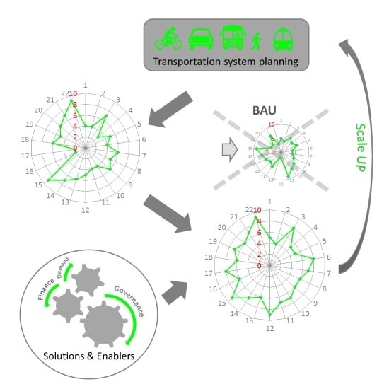
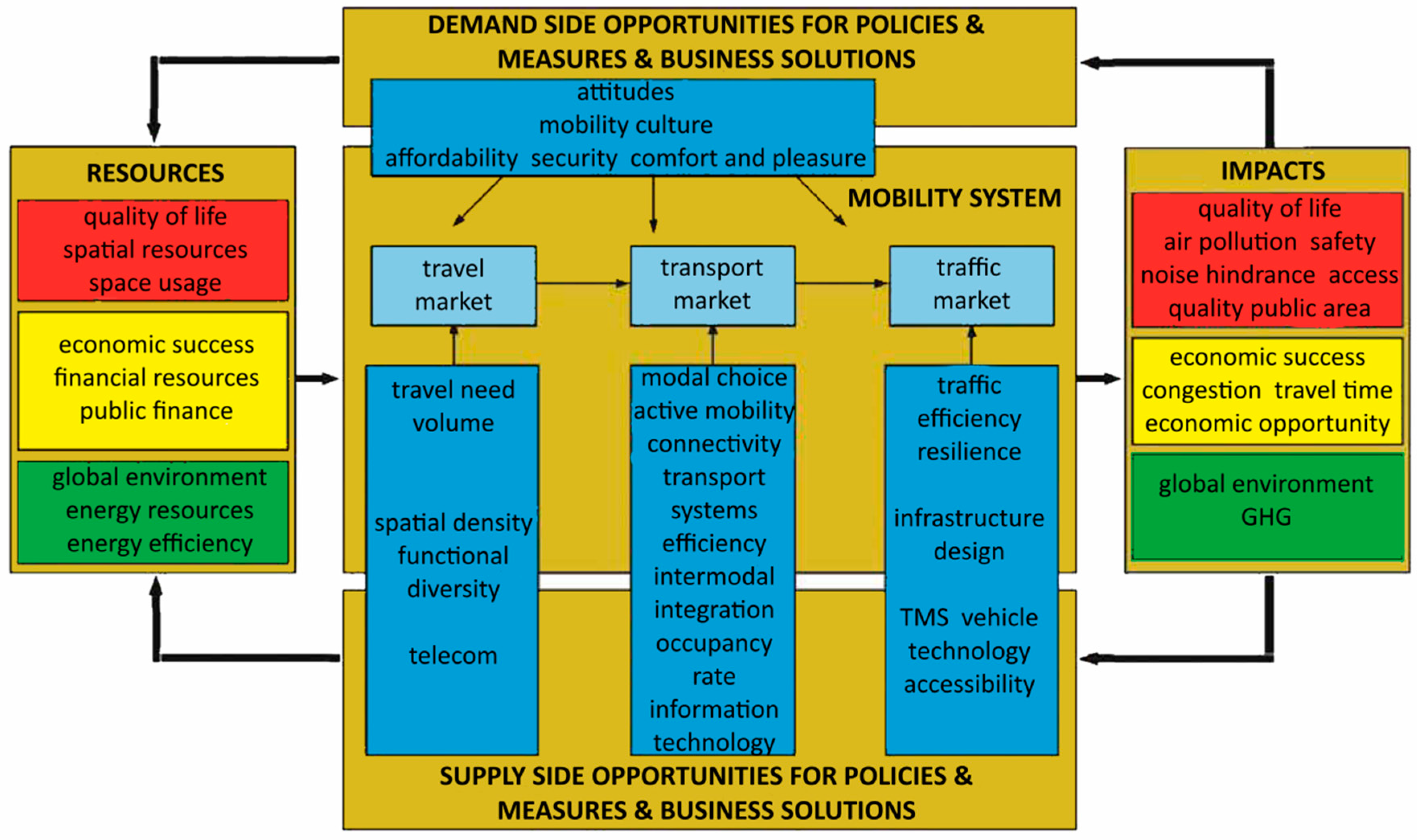

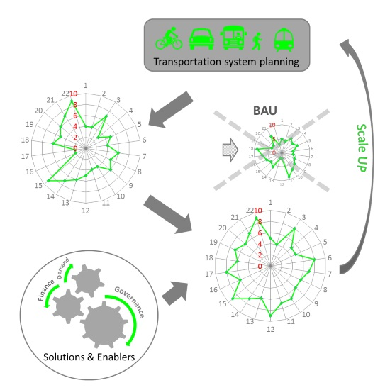