1. Introduction
The outdoor air pollution which accompanied China’s urbanization and industrial development presently constitutes one of the country’s most serious environmental problems [
1]. In fact, sufficient evidence now exists to prove that exposure to outdoor air pollution in itself constitutes a health hazard in China [
2]. Contributing to 1.2 million premature deaths in 2010 and 1.6 million premature deaths in 2014, ambient particulate matter pollution has become the fourth greatest risk factor in all deaths in China, behind only dietary risks, high blood pressure, and smoking [
3,
4,
5]. Beyond the unacceptable cost in human lives, between 2000 and 2010, the economic cost of air quality degradation in China amounted to approximately 6.5% of Chinese GDP annually [
6]. Given these worrying statistics, China faces an arduous task in addressing the challenges presented by air pollution.
A complex process involving significant demographic change, intensified economic activity, and induced variations in extensive land cover and traffic patterns, urbanization plays a significant role in relation to air quality, especially in developing regions [
7,
8,
9,
10]. China underwent rapid urbanization as the result of the country’s shift towards an industrial economy following the reform and “opening up” policies of the 1980s. The permanent urban population in China increased from 17.9% to a staggering 54.77% between 1978 to 2014; ten million people a year migrated from rural areas to China’s large cities during this period, a movement of people that probably constitutes the largest migration in human history [
11]. In association with this growth, in 2010, the country became the world’s second largest economy in terms of its gross domestic product (GDP), after only the year before becoming the world’s biggest energy consumer. This unprecedented scale and accelerated rate of China’s urbanization, linked to the country’s energy consumption, has led to serious resource, energy, and environmental crises, and significant increases in air pollutant and carbon dioxide emissions in the past three decades [
1,
12]. Given that China’s urbanization trend is likely to continue for another 30 years [
13,
14], the conflict between urbanization and the atmospheric environment is likely to continue into the foreseeable future.
The presence of persistent smog and high levels of fine particulates (PM2.5) have acted as a tipping point for China’s clean air movement in recent years, which has been increasingly active in stimulating debates about these issues among the urban Chinese public, the government, academia, and the media [
15,
16]. The current Chinese government has begun to realize the seriousness of the country’s environment problems, and has proposed a “people-oriented, new-type urbanization strategy” for balancing the speed and the quality of urbanization and coordinating the relationship between human and nature [
17,
18]. In 2013, the government’s environment department issued the
Air Pollution Prevention and Control Action Plan (2013–2017) and the Chinese new Air Quality Index, or AQI. The AQI considers six pollutants (PM10, PM2.5, NO
2, SO
2, CO, and O
3), which—compared with its predecessor, the API (Air Pollution Index)—added PM2.5, O
3, and CO. China’s AQI is divided into six grades: good, moderate, unhealthy for sensitive groups, unhealthy, very unhealthy, and hazardous. Regrettably, there were, on average, 73 days characterized by “unhealthy” or worse air quality (
i.e., AQI > 150) in 70 major cities in 2014, and the dominant pollutants present were PM2.5, PM10, and O
3.
Air quality exhibits marked regional differences at the city scale [
19]. What, then, are the factors that are behind these differences and what role does urbanization play? Scholars undertaking work in fields spanning from the humanities to the physical sciences have begun to engage with these critical questions through studies of natural and human factors on air quality. Having reviewed this previous literature, we contend that existing studies have focused excessively on natural factors in recent years. A number of studies regarding, for instance, the impact of local climate and meteorological parameters on air quality—either more generally [
20,
21] or specifically in terms of factors like temperature, wind speed, mixing height, and relative humidity [
22,
23,
24], or changes in mid-latitude cyclone and synoptic weather patterns with climate change [
25,
26,
27].
This is not to say that human factors have not been addressed in research on air quality—for instance, studies have been undertaken on the potential impacts of city vehicles [
28,
29], energy use [
30,
31], population gathering [
19,
32,
33], anthropogenic heat [
34], industrial activities [
35], urban sprawl [
36,
37], and urbanization rate [
38]. Similarly, the urban landscape and land cover have also been identified as important factors [
39], along with changes in land-use patterns [
40] and urban impervious surface [
24,
41]. However, these existing studies are highly specific, considering limited aspects of urbanization. A comprehensive evaluation of the impact of urbanization on air quality is thus required. In particular, we note that imbalances in urban development affect urban air quality indexes [
42]; most of the current research has, however, ignored the spatiality of such imbalances, thereby failing to address spatial dependence and heterogeneity.
In response to this identified deficiency, in the present study, we collected air quality index (AQI) records and urbanization indexes for 289 Chinese cities, posing the following research questions in relation to this data: (1) What is the spatial pattern of China’s air pollution at the city level? (2) How can we evaluate the comprehensive influence of urbanization and identify the impact of significant variables on air quality, quantitatively? (3) To what extent does the spatial contribution made by various urbanization factors account for variations in AQI values? The results from this study, we argue, could constitute a valuable reference for mid-to-long-term environmental policy making in diverse parts of China, and could further assist in improving the quality of the results of future Chinese urbanization.
3. Methodology
Many studies have shown that air pollution emissions exhibits an inverted-U relationship in relation to both economic development and urbanization—this is referred to as the Environmental Kuznets Curve, or EKC [
54,
55]. Despite this general pattern, most parts of China have not reached the inflection points of an EKC [
56], and whilst levels of sulfur dioxide and particulate pollution show some signs of diminishing, nitrogen dioxide levels have in fact increased [
57]. This illustrates that both air quality and the impact of urbanization exhibit obvious “spatial heterogeneity” (
i.e., the presence of variation or instability in space) and complexity. In addition, from existing experience, we know that air pollution has a strongly trans-regional character: it inevitably affects neighboring regions, a quality which can be described in terms of “spatial autocorrelation” in the data. All of these characteristics break with the basic precondition for classical regression analysis, which holds that the samples analyzed must be independent. If we undertake OLS estimation under these circumstances, the results are in fact likely to be biased [
58].
3.1. Measures of Spatial Dependence and Heterogeneity
According to Tobler’s first law of geography, everything is related to everything else, but near things are more related than distant things [
59]. Spatial dependence (or autocorrelation) is thus a fundamental property of all attributes located in space. Global Moran’s
I and local Moran’s
I are measures of spatial autorrelation that indicate whether a variable exhibits significant spatial dependence and heterogeneity quantitatively at a given scale—in this case, whether an AQI value does so at the city scale [
60]. Global Moran’s
I can be expressed as:
where,
n is the number of cities;
xi,
xj is the AQI of spatial location
i,
j; and
S denotes the standard deviation of samples.
Formally, the membership of observations in the neighborhood set for each location is expressed by means of a spatial weights matrix (i.e., Wij). The range of values of global Moran’s I is [–1, 1]. The Z-score is used to test the significance of any spatial autocorrelation. When Z > 2.58(1.96), this usually indicates a positive autocorrelation in the observations at the confidence coefficient of 99% (95%)—i.e., the existence of either high-value or low-value clustering. A significant and negative value, Z < −2.58(−1.96), usually indicates a negative autocorrelation—e.g., a tendency toward the juxtaposition of high values with low values. If I and Z are both close to 0 if n is large, this indicates that the observations display qualities of spatial randomness (i.e., there is no spatial dependence between variables).
To measure and test the spatial heterogeneity and the abnormal value of our results, and given the focus of our study, we adopted Anselin’s LISA (Local Indicators of Spatial Association) technique, using local Moran’s
I to measure significant spatial autocorrelation for each location [
61,
62]. We then visualized the spatial clusters, hot-spots, and outliers using ArcGIS 10.2 [
63]. A local Moran’s
I autocorrelation statistic at the location
i can be expressed as:
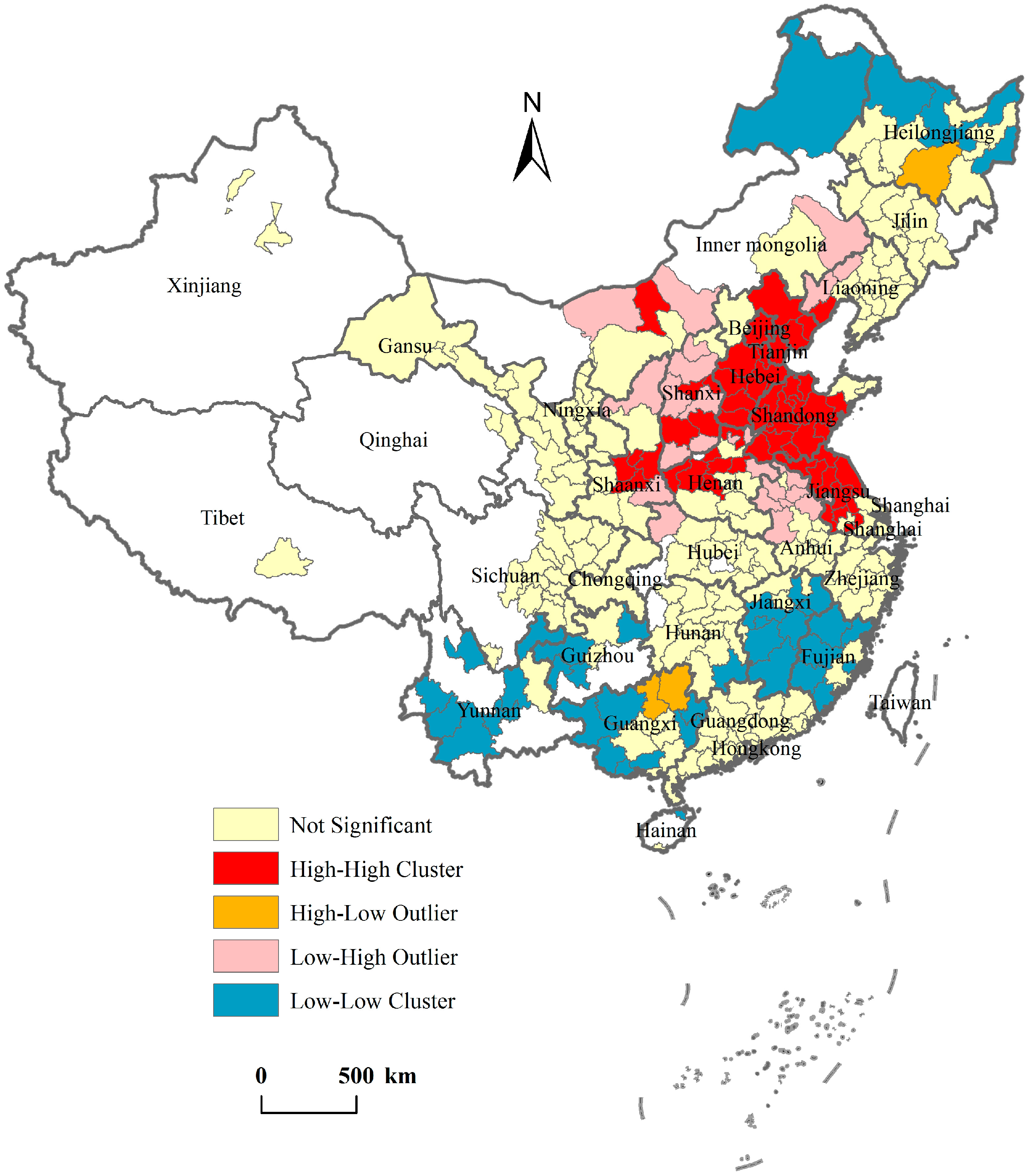
The same significance test was used in relation to local and global clusters. Spatial clusters include high–high clusters (high values in a high-value neighborhood) and low–low clusters (low values in a low-value neighborhood). LISA can thus reveal the presence of hot spots (high–high clusters) and of cool spots (low–low clusters) in terms of the values being studied (in this case, AQI values).
3.2. Spatial Regression Models
If spatial autocorrelation and heterogeneity exist in the spatial units being addressed, an appropriate spatial regression model must be chosen. Spatial regression models allow researchers to account for dependence among their observations, which often arises when observations are collected from points or regions located in space [
64]. The spatial lag model (SAR) and spatial error model (SEM) are spatially constant coefficient models that can be used to produce a spatial extension of OLS, thereby correcting certain spatial dependence problems. The geographically weighted regression (GWR) can be used to produce a spatially varying coefficient model, thereby solving spatial non-stationarity.
3.2.1. Spatial Lag Model (SAR) and Spatial Error Model (SEM)
Choosing the most appropriate spatially constant coefficient model for this research was not without its problems. Formally, the conventional global regression model (that is, using the OLS method of estimation) is the most well known of all regression techniques. This type of regression is known as “global” because of the spatial stationarity of its coefficient estimates, meaning that a single model can be applied equally to different areas of interest. The OLS can be expressed as:
where
xi and
y are, respectively, the independent and dependent variables;
k is the number of independent variables;
β0 is the intercept;
βi is the parameter estimate (coefficient) for the independent variable
xi; and
ɛ is the error term. In Equation (7), the parameter estimates
βi are assumed to be spatially stationary.
When spatial dependence is suspected in the error terms, the SEM is particularly suitable [
65]. The SEM model can be expressed as Equation (8).
where
y is a (N × 1) vector of the dependent variable; X is a (N × K) matrix of the K explanatory variables;
β is a (K × 1) vector of parameters;
u is a (N × 1) vector of residuals; λ is the spatial autocorrelation parameter;
W is a (N × N) spatial-weight matrix or neighborhood connectivity matrix; and ε is a vector of normally distributed errors.
Use of the SAR model is appropriate when spatial dependence is suspected in the values of the dependent variable, an occurrence that can give rise to auto-regressive problems. The SAR model can be expressed as:
where
ρ is the auto-regressive parameter, and spatial lag (
W) as a smoother is the weighted average of neighboring values.
For the spatial econometric models of SAR and SEM, maximum likelihood (ML) estimation allows for efficient estimation of cross-section data in a spatial econometric model [
66]. To determine which model is more appropriate, two Lagrange Multiplier tests are possible: LM (lag) can be used in relation to an autoregressive spatial lag variable, and LM (error) in relation to the spatial autocorrelation of errors. The two robust tests R-LM (lag) and R-LM (error) have a good power against their specific alternative [
67].
3.2.2. Geographically Weighted Regression (GWR)
To address the issue of complex spatial parametric variation or spatial heterogeneity, Fotheringham
et al. have proposed a simple but powerful method called geographically weighted regression (GWR), which extends the OLS to give all the elements and diagnostics of a regression model—such as parameter estimates, goodness-of-fit measures (
R2), and
t-values—on a local basis [
68]. An effective, spatially varying coefficient model, GWR has been widely used in both socioeconomic [
69,
70] and eco-environmental fields [
71,
72,
73], generating results that can be displayed in a spatial map through use of GIS [
74]. The GWR model extends the conventional global regression of Equation (7) by adding a geographical location parameter, and can be expressed as:
where
uj and
vj are the coordinates of location
j;
β0 (
uj,
vj) acts as intercept for location
j; and
βi (
uj,
vj) is the local estimated coefficient for independent variable
xi.
Based on the established concept of distance decay, GWR is calibrated by weighting all observations around a sample point, assuming that the observations closer to the location of the sample point have a higher impact on the local parameter estimates for the location [
74]. A Gaussian distance decay weighting can be used to express the weight function:
where
Wij is the weight for observation
j within the neighborhood of observation
i;
dij denotes the distance between observations
i and
j; and
h represents the kernel bandwidth, which controls the smooth degree of local regression. If the distance is greater than the kernel bandwidth, the weight rapidly approaches zero. GWR is sensitive to kernel bandwidth, and the optimal bandwidth can be chosen by minimizing the corrected Akaike Information Criterion, or AIC [
64].
In this study, when we compared the different models, goodness of fit tests, Log likelihood (LK), and Akaike’s Information Criteria were all used. OLS, SAR, and SEM were carried out using Geoda 1.6. GWR and map visualization was made using ArcGIS 10.2.
5. Conclusions and Policy Implications
5.1. Conclusions
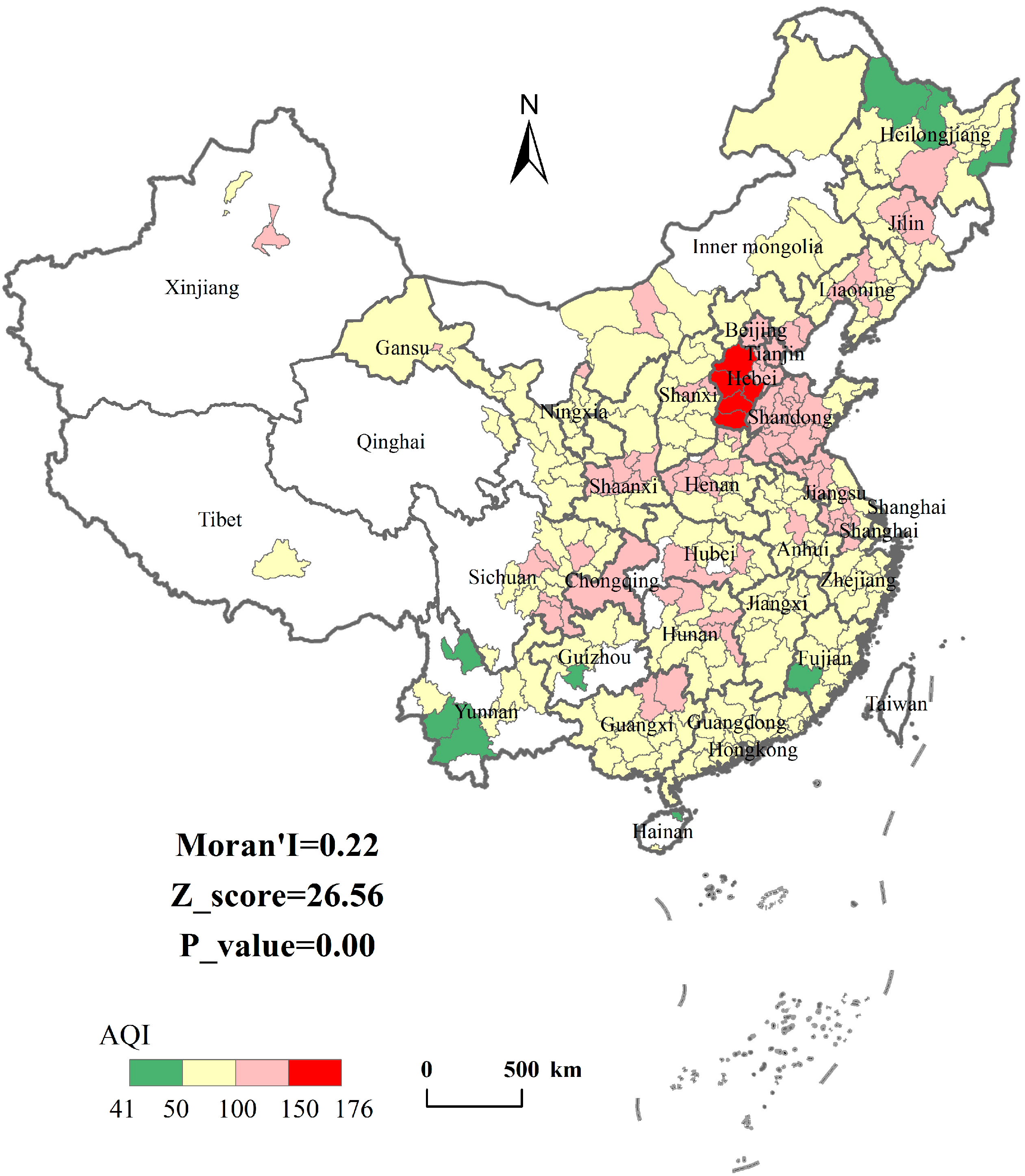
This study first analyzed the spatial pattern of air quality in 289 cities in China, based on Air Quality Index (AQI) records from 2014. Using OLS, SAR, and GWR models, we quantitatively estimated the impact of China’s urbanization processes on air quality, highlighting and exploring the spatial contribution made by a range of urbanization factors in relation to variations in AQI values. We found the AQI of 96.89% of the cities studied to be larger than 50 in 2014, subsequently identifying a significant and strongly positive spatial dependence and heterogeneity in AQI values at the city level. Seriously polluted cities were found to be gathered closely together in Beijing, Tianjin, Hebei, Henan, and Shandong, which presented as hot spots on the visualizations.
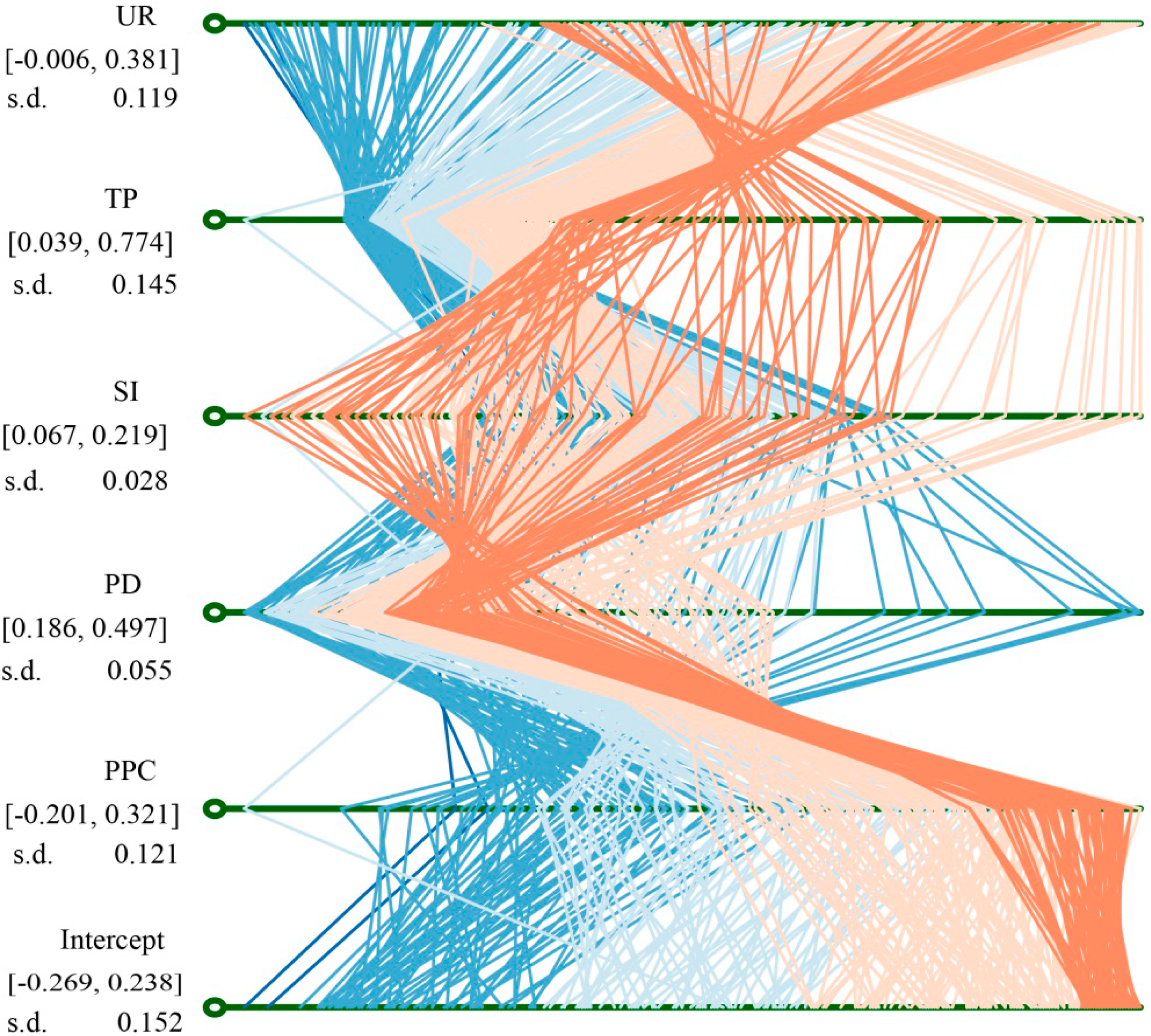
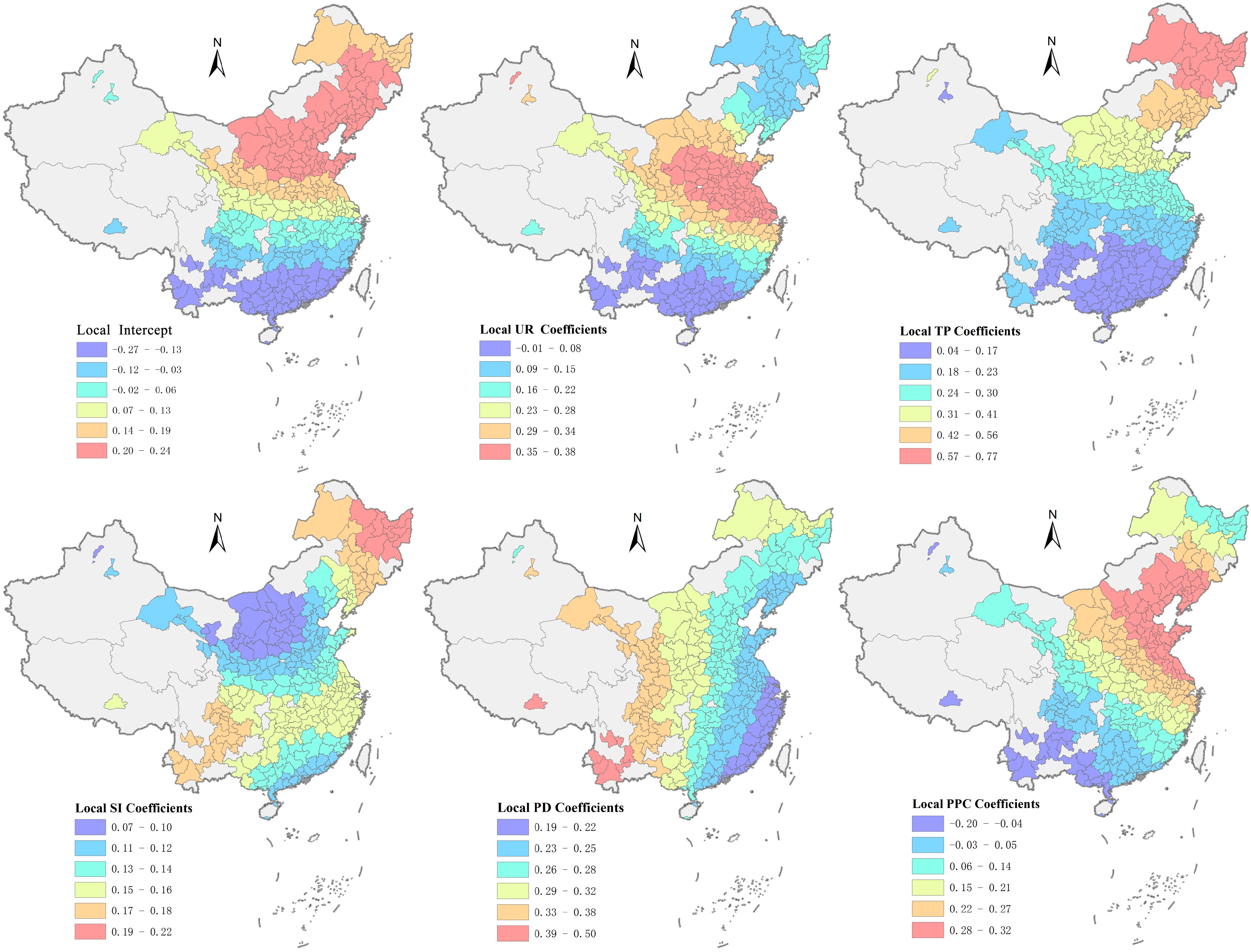
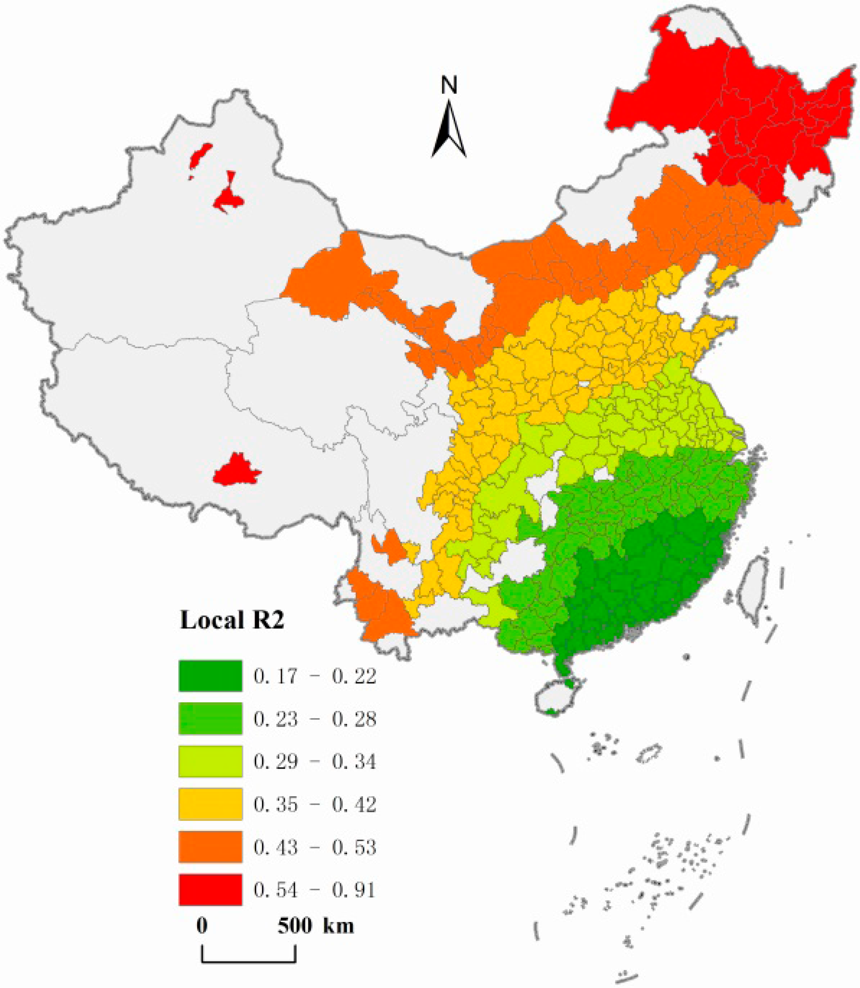
Regression models revealed that all the seven explanatory variables used to depict the urbanization process in fact exerted a negative effect in relation to air quality. The interpretation degree of the R2 reached between 38% and 49.5%, confirming that, with the exclusion of natural factors, urbanization plays an important role in determining air quality. Among the variables, the population, urbanization rate, automobile density, and the proportion of secondary industry were all found to have had a significant influence over air quality. The area of urban development land and per capita GDP, in contrast, failed the significance test at 10% level although they maintained a remarkable correlation with AQI. The results of Moran’s I and SAR modeling indicated that the AQI value of a city can be attributed not only to influencing factors stemming from the city itself but also that of neighboring cities. The GWR results showed that the relationship of urbanization to air quality was not constant over space, but rather varied, with relations being more accurately captured by the regression model in the northern and western areas. The visualization of local parameter estimates highlighted the great spatial variation, which exists in the impact exerted by different urbanization factors in relation to different regional AQI values. These results also reinforce the complementary nature of these methods: the OLS (and SAR) results provided needed context for the GWR model, and the GWR was able to be used for simulating air quality in a manner that could take into account spatial dependence and heterogeneity.
In addition, these results should be generalized with caution, and it is emphasized that the present study only addresses the Chinese context. Whether the results of the study are suitable for other developing countries constitutes a matter for further examination. Considering the strong linkage exposed here between natural factors and air quality, it recognized that is also necessary to integrate natural and urbanization-related factors, and a comprehensive mechanism should thus be developed for such an operation through the future research.
5.2. Policy Implications
With the rate and scale of urbanization expected to drastically increase in the next 30 years, Chinese government officials face serious challenges in addressing the issue of air pollution. Through this paper, we propose several suggestions based on the empirical results:
Firstly, this study provides scientific validation for the presence of a strong spatial dependence in air quality at the city scale mainly because of the atmospheric flow. On the other hand, the pollutants are generated not only stationary sources (e.g., industry) but also non-stationary sources (e.g., vehicles). As such, we should take into full account spatial factors and policies must be directed at the source, increasing awareness of regional environmental systems. Air pollution prevention and control should be coordinated, with complementary measures undertaken across adjacent regions, especially in the urban agglomerations (e.g., Beijing-Tianjin-Hebei).
Secondly, because overall population density and total population play the most important roles in determining air quality, from the perspective of improving the country’s urban air quality, China must strictly control the scale of megacities and actively develop small and medium-sized cities. Automobile density and the proportion of secondary industry has significant impacts in relation to AQI values: thus, on the one hand, China must promote intelligent traffic management, increase the proportion of green public transport and reasonably controlling the vehicle population in order to reduce emissions from transport; on the other, more attention needs to be paid to accelerating the adjustment and transformation of the country’s industrial structure, accelerating the elimination of lagging productivity, and reducing dependence on coal.
Thirdly, we should fully acknowledge the spatial dependence and heterogeneity present in the relation between various parameters of urbanization and air quality in different geographic areas in China. Regional inequality between Chinese cities in terms of both urbanization and economic development is very large [
76], and regionally specific policy analysis should be undertaken by local governments with respect to the various influence mechanisms exerted by urbanization on the atmospheric environment. The macroscopic environment policy of the central government should ultimately act to balance these regional differences on the basis of the understanding that “one size does not fit all”.


