Estimating the Impact of Urbanization on Air Quality in China Using Spatial Regression Models

Abstract

Urban air pollution is one of the most visible environmental problems to have accompanied China’s rapid urbanization. Based on emission inventory data from 2014, gathered from 289 cities, we used Global and Local Moran’s I to measure the spatial autorrelation of Air Quality Index (AQI) values at the city level, and employed Ordinary Least Squares (OLS), Spatial Lag Model (SAR), and Geographically Weighted Regression (GWR) to quantitatively estimate the comprehensive impact and spatial variations of China’s urbanization process on air quality. The results show that a significant spatial dependence and heterogeneity existed in AQI values. Regression models revealed urbanization has played an important negative role in determining air quality in Chinese cities. The population, urbanization rate, automobile density, and the proportion of secondary industry were all found to have had a significant influence over air quality. Per capita Gross Domestic Product (GDP) and the scale of urban land use, however, failed the significance test at 10% level. The GWR model performed better than global models and the results of GWR modeling show that the relationship between urbanization and air quality was not constant in space. Further, the local parameter estimates suggest significant spatial variation in the impacts of various urbanization factors on air quality.

1. Introduction

The outdoor air pollution which accompanied China’s urbanization and industrial development presently constitutes one of the country’s most serious environmental problems [1]. In fact, sufficient evidence now exists to prove that exposure to outdoor air pollution in itself constitutes a health hazard in China [2]. Contributing to 1.2 million premature deaths in 2010 and 1.6 million premature deaths in 2014, ambient particulate matter pollution has become the fourth greatest risk factor in all deaths in China, behind only dietary risks, high blood pressure, and smoking [3,4,5]. Beyond the unacceptable cost in human lives, between 2000 and 2010, the economic cost of air quality degradation in China amounted to approximately 6.5% of Chinese GDP annually [6]. Given these worrying statistics, China faces an arduous task in addressing the challenges presented by air pollution.

A complex process involving significant demographic change, intensified economic activity, and induced variations in extensive land cover and traffic patterns, urbanization plays a significant role in relation to air quality, especially in developing regions [7,8,9,10]. China underwent rapid urbanization as the result of the country’s shift towards an industrial economy following the reform and “opening up” policies of the 1980s. The permanent urban population in China increased from 17.9% to a staggering 54.77% between 1978 to 2014; ten million people a year migrated from rural areas to China’s large cities during this period, a movement of people that probably constitutes the largest migration in human history [11]. In association with this growth, in 2010, the country became the world’s second largest economy in terms of its gross domestic product (GDP), after only the year before becoming the world’s biggest energy consumer. This unprecedented scale and accelerated rate of China’s urbanization, linked to the country’s energy consumption, has led to serious resource, energy, and environmental crises, and significant increases in air pollutant and carbon dioxide emissions in the past three decades [1,12]. Given that China’s urbanization trend is likely to continue for another 30 years [13,14], the conflict between urbanization and the atmospheric environment is likely to continue into the foreseeable future.

The presence of persistent smog and high levels of fine particulates (PM2.5) have acted as a tipping point for China’s clean air movement in recent years, which has been increasingly active in stimulating debates about these issues among the urban Chinese public, the government, academia, and the media [15,16]. The current Chinese government has begun to realize the seriousness of the country’s environment problems, and has proposed a “people-oriented, new-type urbanization strategy” for balancing the speed and the quality of urbanization and coordinating the relationship between human and nature [17,18]. In 2013, the government’s environment department issued the Air Pollution Prevention and Control Action Plan (2013–2017) and the Chinese new Air Quality Index, or AQI. The AQI considers six pollutants (PM10, PM2.5, NO₂, SO₂, CO, and O₃), which—compared with its predecessor, the API (Air Pollution Index)—added PM2.5, O₃, and CO. China’s AQI is divided into six grades: good, moderate, unhealthy for sensitive groups, unhealthy, very unhealthy, and hazardous. Regrettably, there were, on average, 73 days characterized by “unhealthy” or worse air quality (i.e., AQI > 150) in 70 major cities in 2014, and the dominant pollutants present were PM2.5, PM10, and O₃.

Air quality exhibits marked regional differences at the city scale [19]. What, then, are the factors that are behind these differences and what role does urbanization play? Scholars undertaking work in fields spanning from the humanities to the physical sciences have begun to engage with these critical questions through studies of natural and human factors on air quality. Having reviewed this previous literature, we contend that existing studies have focused excessively on natural factors in recent years. A number of studies regarding, for instance, the impact of local climate and meteorological parameters on air quality—either more generally [20,21] or specifically in terms of factors like temperature, wind speed, mixing height, and relative humidity [22,23,24], or changes in mid-latitude cyclone and synoptic weather patterns with climate change [25,26,27].

This is not to say that human factors have not been addressed in research on air quality—for instance, studies have been undertaken on the potential impacts of city vehicles [28,29], energy use [30,31], population gathering [19,32,33], anthropogenic heat [34], industrial activities [35], urban sprawl [36,37], and urbanization rate [38]. Similarly, the urban landscape and land cover have also been identified as important factors [39], along with changes in land-use patterns [40] and urban impervious surface [24,41]. However, these existing studies are highly specific, considering limited aspects of urbanization. A comprehensive evaluation of the impact of urbanization on air quality is thus required. In particular, we note that imbalances in urban development affect urban air quality indexes [42]; most of the current research has, however, ignored the spatiality of such imbalances, thereby failing to address spatial dependence and heterogeneity.

In response to this identified deficiency, in the present study, we collected air quality index (AQI) records and urbanization indexes for 289 Chinese cities, posing the following research questions in relation to this data: (1) What is the spatial pattern of China’s air pollution at the city level? (2) How can we evaluate the comprehensive influence of urbanization and identify the impact of significant variables on air quality, quantitatively? (3) To what extent does the spatial contribution made by various urbanization factors account for variations in AQI values? The results from this study, we argue, could constitute a valuable reference for mid-to-long-term environmental policy making in diverse parts of China, and could further assist in improving the quality of the results of future Chinese urbanization.

2. Data

2.1. AQI Record

An Air Quality Index (AQI) integrates a range of air pollutant measures. This dimensionless index is widely used to comprehensively reflect atmospheric pollution, as well as potential effects on citizens’ health, in a range of countries. Air quality monitoring systems in China have been installed in 338 cities, including 1436 monitoring sites in 2015. The new version of AQI was made available in about 300 prefecture-level cities in 2014 [43]; these values represent the maximum pollution sub index of six individual pollutants (SO₂, NO₂, PM10, PM2.5, O₃, CO), and are calculated as follows:

$$AQI=\max (IAQ{I}_1,IAQ{I}_2,\dots ,IAQ{I}_n）$$

(1)

$$IAQ{I}_p=\frac{IAQ{I}_{Hi}-IAQ{I}_{Lo}}{C_{Hi}-C_{Lo}}（C_p-C_{Lo}）+IAQ{I}_{Lo}$$

(2)

where IAQI_p is the air quality sub index for pollutant p; C_p is the concentration of pollutant p; C_lo is the concentration breakpoint that is ≤C; C_hi is the concentration breakpoint that is ≥C; IAQI_lo is the index breakpoint corresponding to C_lo; and IAQI_hi is the index breakpoint corresponding to C_hi.

It is necessary to note that different countries each have their own air quality indices, which correspond to specific national air quality standards. In the process of formulating such standards, the World Health Organization (WHO) Air Quality Guidelines are usually referenced [44], which focus on minimum particle concentrations. Considering the developmental stage of socioeconomic conditions in China, as well as the priority that is placed upon public health [45], the concentration breakpoint of China’s IAQI is set at the WHO’s recommended interim target (Table 1). Considering the availability and consistency of data, this study used the annual mean AQI value for each of the 289 cities (285 prefecture-level cities and four municipalities) for the year 2014. The raw daily data of AQI came from ministry of environmental protection of China [43]. What we should note here is that because the monitoring sites are concentrated in the urban area, the AQI value reflect the air environment of population exposure region. On the other hand, there are likely errors with the measurements if we want to know the average value within the whole area.

Table 1. Pollutant-specific sub-indices of the Air Quality Index (AQI) in China.

AQI Categories (Index Values)	SO2 (μg/m3, 24-h)	NO2 (μg/m3, 24-h)	CO (μg/m3, 24-h)	O3 (μg/m3, 1-h)	PM2.5 (μg/m3, 24-h)	PM10 (μg/m3, 24-h)
Good (Up to 50)	0–50	0–40	0–2	0–160	0–35	0–50
Moderate (51–100)	51–150	41–80	3–4	161–200	35–75	51–150
Unhealthy for Sensitive Groups (101–150)	151–475	81–180	5–14	201–300	75–115	151–250
Unhealthy (151–200)	476–800	181–280	15–24	301–400	115–150	251–350
Very Unhealthy (201–300)	801–1600	281–565	25–36	401–800	150–250	351–420
Hazardous (301–500)	1601–2620	566–940	37–60	801–1200	250–500	421–600

Note: Daily urban air quality uses 24-h average concentration limit of pollutants except O₃, and the IAQI of O₃ uses 1-h average concentration.

Table 1. Pollutant-specific sub-indices of the Air Quality Index (AQI) in China.

AQI Categories (Index Values)	SO2 (μg/m3, 24-h)	NO2 (μg/m3, 24-h)	CO (μg/m3, 24-h)	O3 (μg/m3, 1-h)	PM2.5 (μg/m3, 24-h)	PM10 (μg/m3, 24-h)
Good (Up to 50)	0–50	0–40	0–2	0–160	0–35	0–50
Moderate (51–100)	51–150	41–80	3–4	161–200	35–75	51–150
Unhealthy for Sensitive Groups (101–150)	151–475	81–180	5–14	201–300	75–115	151–250
Unhealthy (151–200)	476–800	181–280	15–24	301–400	115–150	251–350
Very Unhealthy (201–300)	801–1600	281–565	25–36	401–800	150–250	351–420
Hazardous (301–500)	1601–2620	566–940	37–60	801–1200	250–500	421–600

Note: Daily urban air quality uses 24-h average concentration limit of pollutants except O₃, and the IAQI of O₃ uses 1-h average concentration.

2.2. Urbanization Index

Urbanization is a comprehensive and complex process, and the interactive coupling between air pollution and urbanization reflects this complexity. The raw data came from the China City Statistical Yearbook 2014 [46] and China’s Regional Economic Statistical Yearbook 2014 [47]. In accordance with previous research [48,49], we divided urbanization into four subsystems: demographic urbanization, economic urbanization, spatial urbanization, and social urbanization. As shown in Table 2, 12 indicators (including the proportion of urban population, per capita GDP, private car ownership, amongst others) were selected in order to build a primary index system able to quantitatively depict the urbanization process as it impacts air quality. These indicators are organized within the four aforementioned urbanization subsystems. Energy-related indicators were deliberately not included in this research due to the strong statistical collinearity. Whilst energy consumption acts as an important index with respect to urbanization and is the primary source of many pollutants [31,50], it affects many aspects of urbanization, including population, GDP, and the proportion of secondary industry [51,52].

Table 2. The primary index system used to reflect the impact of urbanization on air quality.

The Subsystem of Urbanization	Index	Acronym Index
Demographic urbanization	The proportion of urban population (%)	UR
	Total population (104 people)	TP
	Non-agricultural population (104 people)	NP
Economic urbanization	Proportion of the added value of secondary industry to GDP (%)	SI
	GDP (104 Yuan)	GDP
	GDP per capita (Yuan)	PGDP
Spatial urbanization	Urban development land (sq km)	UL
	Population density (people/sq km)	PD
	Urban development land per capita (m2/people)	PUL
Social urbanization	Private car ownership	PC
	Private cars per unit of urban development land	PPC
	Total retail sales of consumer goods (108 Yuan)	TG

Table 2. The primary index system used to reflect the impact of urbanization on air quality.

The Subsystem of Urbanization	Index	Acronym Index
Demographic urbanization	The proportion of urban population (%)	UR
	Total population (104 people)	TP
	Non-agricultural population (104 people)	NP
Economic urbanization	Proportion of the added value of secondary industry to GDP (%)	SI
	GDP (104 Yuan)	GDP
	GDP per capita (Yuan)	PGDP
Spatial urbanization	Urban development land (sq km)	UL
	Population density (people/sq km)	PD
	Urban development land per capita (m2/people)	PUL
Social urbanization	Private car ownership	PC
	Private cars per unit of urban development land	PPC
	Total retail sales of consumer goods (108 Yuan)	TG

2.3. Variable Selection and Data Pre-Processing

Multicollinearity is a state of very high intercorrelation or inter-association among the independent variables in a regression model; it can play havoc with an analysis, generating misleading results for regression coefficients and standard errors [53]. Multicollinearity can be detected with the help of a variance inflation factor (VIF). A VIF value of 10 or above indicates that the level of multicollinearity is problematic. In order to ensure that proper explanatory variables were used in the ordinary least squares (OLS) regression, we removed the independent variables whose VIF > 10, one by one, until multicollinearity disappeared entirely. We were then left with seven explanatory variables (UR, TP, SI, PGDP, UL, PD, PPC), between which there existed no obvious correlation (Table 3). We subsequently undertook a correlation analysis of each of these seven variables and the AQI values for the 289 cities, the results of which suggested that Spearman’s correlations were all significant at the 5% significance level (Table 4).

Table 3. Descriptive statistics of the independent variables.

Variables	Minimum	Maximum	Mean	Standard Error	Standard Deviation
AQI	41.15	175.70	84.53	1.47	25.06
UR	10.46	100.00	38.52	1.20	20.36
TP	20.00	2970.00	440.82	17.71	301.06
UL	13.00	2915.56	133.65	13.30	226.16
SI	17.48	79.36	50.78	0.59	9.99
PD	14.57	8248.04	901.04	50.15	852.51
PGDP	8404.47	466,996.14	51,233.46	2834.88	48,192.94
PPC	310.00	15,426.00	3595.79	139.27	2367.57

Table 3. Descriptive statistics of the independent variables.

Variables	Minimum	Maximum	Mean	Standard Error	Standard Deviation
AQI	41.15	175.70	84.53	1.47	25.06
UR	10.46	100.00	38.52	1.20	20.36
TP	20.00	2970.00	440.82	17.71	301.06
UL	13.00	2915.56	133.65	13.30	226.16
SI	17.48	79.36	50.78	0.59	9.99
PD	14.57	8248.04	901.04	50.15	852.51
PGDP	8404.47	466,996.14	51,233.46	2834.88	48,192.94
PPC	310.00	15,426.00	3595.79	139.27	2367.57

Table 4. Spearman’s correlation of the independent variables and AQI.

		AQI	UR	TP	UL	SI	PD	PGDP	PPC
AQI	Spearman’s correlation	1.00	0.199 **	0.367 **	0.254 **	0.171 **	0.459 **	0.207 **	0.134 *
	sig.(2-tailed)		0.00	0.00	0.00	0.00	0.00	0.00	0.02
UR	Spearman’s correlation	0.199 **	1.00	−0.09	0.437 **	0.08	0.08	0.611 **	−0.326 **
	sig.(2-tailed)	0.00		0.15	0.00	0.18	0.16	0.00	0.00
TP	Spearman’s correlation	0.367 **	−0.09	1.00	0.483 **	−0.177 **	0.351 **	−0.06	0.194 **
	sig.(2-tailed)	0.00	0.15		0.00	0.00	0.00	0.35	0.00
UL	Spearman’s correlation	0.254 **	0.437 **	0.483 **	1.00	−0.155 **	0.244 **	0.456 **	−0.151 *
	sig.(2-tailed)	0.00	0.00	0.00		0.01	0.00	0.00	0.01
SI	Spearman’s correlation	0.171 **	0.08	−0.177 **	−0.155 **	1.00	0.149 *	0.149 *	−0.03
	sig.(2-tailed)	0.00	0.18	0.00	0.01		0.01	0.01	0.57
PD	Spearman’s correlation	0.459 **	0.08	0.351 **	0.244 **	0.149 *	1.00	0.09	0.09
	sig.(2-tailed)	0.00	0.16	0.00	0.00	0.01		0.13	0.11
PGDP	Spearman’s correlation	0.207 **	0.611 **	−0.06	0.456 **	0.149 *	0.09	1.00	−0.06
	sig.(2-tailed)	0.00	0.00	0.35	0.00	0.01	0.13		0.29
PPC	Spearman’s correlation	0.134 *	−0.326 **	0.194 **	−0.151 *	−0.03	0.09	−0.06	1.00
	sig.(2-tailed)	0.02	0.00	0.00	0.01	0.57	0.11	0.29

Note: **, or * indicates significance at 1% or 5% levels respectively. Number of samples: 289.

Table 4. Spearman’s correlation of the independent variables and AQI.

		AQI	UR	TP	UL	SI	PD	PGDP	PPC
AQI	Spearman’s correlation	1.00	0.199 **	0.367 **	0.254 **	0.171 **	0.459 **	0.207 **	0.134 *
	sig.(2-tailed)		0.00	0.00	0.00	0.00	0.00	0.00	0.02
UR	Spearman’s correlation	0.199 **	1.00	−0.09	0.437 **	0.08	0.08	0.611 **	−0.326 **
	sig.(2-tailed)	0.00		0.15	0.00	0.18	0.16	0.00	0.00
TP	Spearman’s correlation	0.367 **	−0.09	1.00	0.483 **	−0.177 **	0.351 **	−0.06	0.194 **
	sig.(2-tailed)	0.00	0.15		0.00	0.00	0.00	0.35	0.00
UL	Spearman’s correlation	0.254 **	0.437 **	0.483 **	1.00	−0.155 **	0.244 **	0.456 **	−0.151 *
	sig.(2-tailed)	0.00	0.00	0.00		0.01	0.00	0.00	0.01
SI	Spearman’s correlation	0.171 **	0.08	−0.177 **	−0.155 **	1.00	0.149 *	0.149 *	−0.03
	sig.(2-tailed)	0.00	0.18	0.00	0.01		0.01	0.01	0.57
PD	Spearman’s correlation	0.459 **	0.08	0.351 **	0.244 **	0.149 *	1.00	0.09	0.09
	sig.(2-tailed)	0.00	0.16	0.00	0.00	0.01		0.13	0.11
PGDP	Spearman’s correlation	0.207 **	0.611 **	−0.06	0.456 **	0.149 *	0.09	1.00	−0.06
	sig.(2-tailed)	0.00	0.00	0.35	0.00	0.01	0.13		0.29
PPC	Spearman’s correlation	0.134 *	−0.326 **	0.194 **	−0.151 *	−0.03	0.09	−0.06	1.00
	sig.(2-tailed)	0.02	0.00	0.00	0.01	0.57	0.11	0.29

Note: **, or * indicates significance at 1% or 5% levels respectively. Number of samples: 289.

In addition, we also undertook a Z-score normalization in relation to the raw data in order to eliminate the influence of unit and order of magnitude, making the data accord better with a normal distribution. The Z-score normalization used can be expressed as:

$$Z=\frac{x_i-\mu }{\sqrt{\sum {(x_i-\mu )}^2/(n-1)}}$$

(3)

where x_i is the raw value of city i, and µ represents the mean of the indicator.

3. Methodology

Many studies have shown that air pollution emissions exhibits an inverted-U relationship in relation to both economic development and urbanization—this is referred to as the Environmental Kuznets Curve, or EKC [54,55]. Despite this general pattern, most parts of China have not reached the inflection points of an EKC [56], and whilst levels of sulfur dioxide and particulate pollution show some signs of diminishing, nitrogen dioxide levels have in fact increased [57]. This illustrates that both air quality and the impact of urbanization exhibit obvious “spatial heterogeneity” (i.e., the presence of variation or instability in space) and complexity. In addition, from existing experience, we know that air pollution has a strongly trans-regional character: it inevitably affects neighboring regions, a quality which can be described in terms of “spatial autocorrelation” in the data. All of these characteristics break with the basic precondition for classical regression analysis, which holds that the samples analyzed must be independent. If we undertake OLS estimation under these circumstances, the results are in fact likely to be biased [58].

3.1. Measures of Spatial Dependence and Heterogeneity

According to Tobler’s first law of geography, everything is related to everything else, but near things are more related than distant things [59]. Spatial dependence (or autocorrelation) is thus a fundamental property of all attributes located in space. Global Moran’s I and local Moran’s I are measures of spatial autorrelation that indicate whether a variable exhibits significant spatial dependence and heterogeneity quantitatively at a given scale—in this case, whether an AQI value does so at the city scale [60]. Global Moran’s I can be expressed as:

$$\mathit{Global}I=\frac{{\displaystyle \sum _{i=1}^n}{\displaystyle \sum _{j\ne i}^n}{W}_{ij}(x_i-\bar{x})(x_j-\bar{x})}{S^2{\displaystyle \sum _{i=1}^n}{\displaystyle \sum _{j\ne i}^n}{W}_{ij}}=\frac{n{\displaystyle \sum _{i=1}^n}{\displaystyle \sum _{j=1}^n}{W}_{ij}(x_i-\bar{x})(x_j-\bar{x})}{{\displaystyle \sum _{i=1}^n}{\displaystyle \sum _{j=1}^n}{W}_{ij}{\displaystyle \sum _{i=1}^n}{(x_i-\bar{x})}^2}$$

(4)

$$Z=\frac{I-E(I)}{\sqrt{VAR(I)}}=\frac{{\displaystyle \sum _{j\ne i}^n}{\mathrm{W}}_{ij}(d)(x_j-{\bar{x}}_i)}{S_i\sqrt{{\mathrm{W}}_i(n-1-{\mathrm{W}}_i)/(n-2)}} j\ne i$$

(5)

where, n is the number of cities; x_i, x_j is the AQI of spatial location i, j; and S denotes the standard deviation of samples.

Formally, the membership of observations in the neighborhood set for each location is expressed by means of a spatial weights matrix (i.e., W_ij). The range of values of global Moran’s I is [–1, 1]. The Z-score is used to test the significance of any spatial autocorrelation. When Z > 2.58(1.96), this usually indicates a positive autocorrelation in the observations at the confidence coefficient of 99% (95%)—i.e., the existence of either high-value or low-value clustering. A significant and negative value, Z < −2.58(−1.96), usually indicates a negative autocorrelation—e.g., a tendency toward the juxtaposition of high values with low values. If I and Z are both close to 0 if n is large, this indicates that the observations display qualities of spatial randomness (i.e., there is no spatial dependence between variables).

To measure and test the spatial heterogeneity and the abnormal value of our results, and given the focus of our study, we adopted Anselin’s LISA (Local Indicators of Spatial Association) technique, using local Moran’s I to measure significant spatial autocorrelation for each location [61,62]. We then visualized the spatial clusters, hot-spots, and outliers using ArcGIS 10.2 [63]. A local Moran’s I autocorrelation statistic at the location i can be expressed as:

$$LocalI=\frac{(x_i-\overline{x})}{S^2}{\displaystyle \sum _j{W}_{ij}(x_j-\overline{x})}$$

(6)

The same significance test was used in relation to local and global clusters. Spatial clusters include high–high clusters (high values in a high-value neighborhood) and low–low clusters (low values in a low-value neighborhood). LISA can thus reveal the presence of hot spots (high–high clusters) and of cool spots (low–low clusters) in terms of the values being studied (in this case, AQI values).

3.2. Spatial Regression Models

If spatial autocorrelation and heterogeneity exist in the spatial units being addressed, an appropriate spatial regression model must be chosen. Spatial regression models allow researchers to account for dependence among their observations, which often arises when observations are collected from points or regions located in space [64]. The spatial lag model (SAR) and spatial error model (SEM) are spatially constant coefficient models that can be used to produce a spatial extension of OLS, thereby correcting certain spatial dependence problems. The geographically weighted regression (GWR) can be used to produce a spatially varying coefficient model, thereby solving spatial non-stationarity.

3.2.1. Spatial Lag Model (SAR) and Spatial Error Model (SEM)

Choosing the most appropriate spatially constant coefficient model for this research was not without its problems. Formally, the conventional global regression model (that is, using the OLS method of estimation) is the most well known of all regression techniques. This type of regression is known as “global” because of the spatial stationarity of its coefficient estimates, meaning that a single model can be applied equally to different areas of interest. The OLS can be expressed as:

$$y={\beta }_0+\sum _{i=1}^k{\beta }_i{x}_i+\epsilon , \epsilon ~N(0, {\delta }^2)$$

(7)

where x_i and y are, respectively, the independent and dependent variables; k is the number of independent variables; β₀ is the intercept; β_i is the parameter estimate (coefficient) for the independent variable x_i; and ɛ is the error term. In Equation (7), the parameter estimates β_i are assumed to be spatially stationary.

When spatial dependence is suspected in the error terms, the SEM is particularly suitable [65]. The SEM model can be expressed as Equation (8).

$$y=X\beta +\lambda Wu+\epsilon ,\epsilon ~N(0,{\delta }^2)$$

(8)

where y is a (N × 1) vector of the dependent variable; X is a (N × K) matrix of the K explanatory variables; β is a (K × 1) vector of parameters; u is a (N × 1) vector of residuals; λ is the spatial autocorrelation parameter; W is a (N × N) spatial-weight matrix or neighborhood connectivity matrix; and ε is a vector of normally distributed errors.

Use of the SAR model is appropriate when spatial dependence is suspected in the values of the dependent variable, an occurrence that can give rise to auto-regressive problems. The SAR model can be expressed as:

$$y=\rho Wy+X\beta +\epsilon ,\epsilon ~N(0,{\delta }^2)$$

(9)

where ρ is the auto-regressive parameter, and spatial lag (W) as a smoother is the weighted average of neighboring values.

For the spatial econometric models of SAR and SEM, maximum likelihood (ML) estimation allows for efficient estimation of cross-section data in a spatial econometric model [66]. To determine which model is more appropriate, two Lagrange Multiplier tests are possible: LM (lag) can be used in relation to an autoregressive spatial lag variable, and LM (error) in relation to the spatial autocorrelation of errors. The two robust tests R-LM (lag) and R-LM (error) have a good power against their specific alternative [67].

3.2.2. Geographically Weighted Regression (GWR)

To address the issue of complex spatial parametric variation or spatial heterogeneity, Fotheringham et al. have proposed a simple but powerful method called geographically weighted regression (GWR), which extends the OLS to give all the elements and diagnostics of a regression model—such as parameter estimates, goodness-of-fit measures (R²), and t-values—on a local basis [68]. An effective, spatially varying coefficient model, GWR has been widely used in both socioeconomic [69,70] and eco-environmental fields [71,72,73], generating results that can be displayed in a spatial map through use of GIS [74]. The GWR model extends the conventional global regression of Equation (7) by adding a geographical location parameter, and can be expressed as:

$$y_j={\beta }_0(u_j,{\upsilon }_j)+\sum _{i=1}^p{\beta }_i(u_j,{\upsilon }_j)x_{ij}+{\epsilon }_j$$

(10)

where uj and vj are the coordinates of location j; β₀ (uj, vj) acts as intercept for location j; and βi (uj, vj) is the local estimated coefficient for independent variable xi.

Based on the established concept of distance decay, GWR is calibrated by weighting all observations around a sample point, assuming that the observations closer to the location of the sample point have a higher impact on the local parameter estimates for the location [74]. A Gaussian distance decay weighting can be used to express the weight function:

$$W_{ij}=\exp (-d_{ij}^2/h^2)$$

(11)

where W_ij is the weight for observation j within the neighborhood of observation i; d_ij denotes the distance between observations i and j; and h represents the kernel bandwidth, which controls the smooth degree of local regression. If the distance is greater than the kernel bandwidth, the weight rapidly approaches zero. GWR is sensitive to kernel bandwidth, and the optimal bandwidth can be chosen by minimizing the corrected Akaike Information Criterion, or AIC [64].

In this study, when we compared the different models, goodness of fit tests, Log likelihood (LK), and Akaike’s Information Criteria were all used. OLS, SAR, and SEM were carried out using Geoda 1.6. GWR and map visualization was made using ArcGIS 10.2.

4. Results and Interpretations

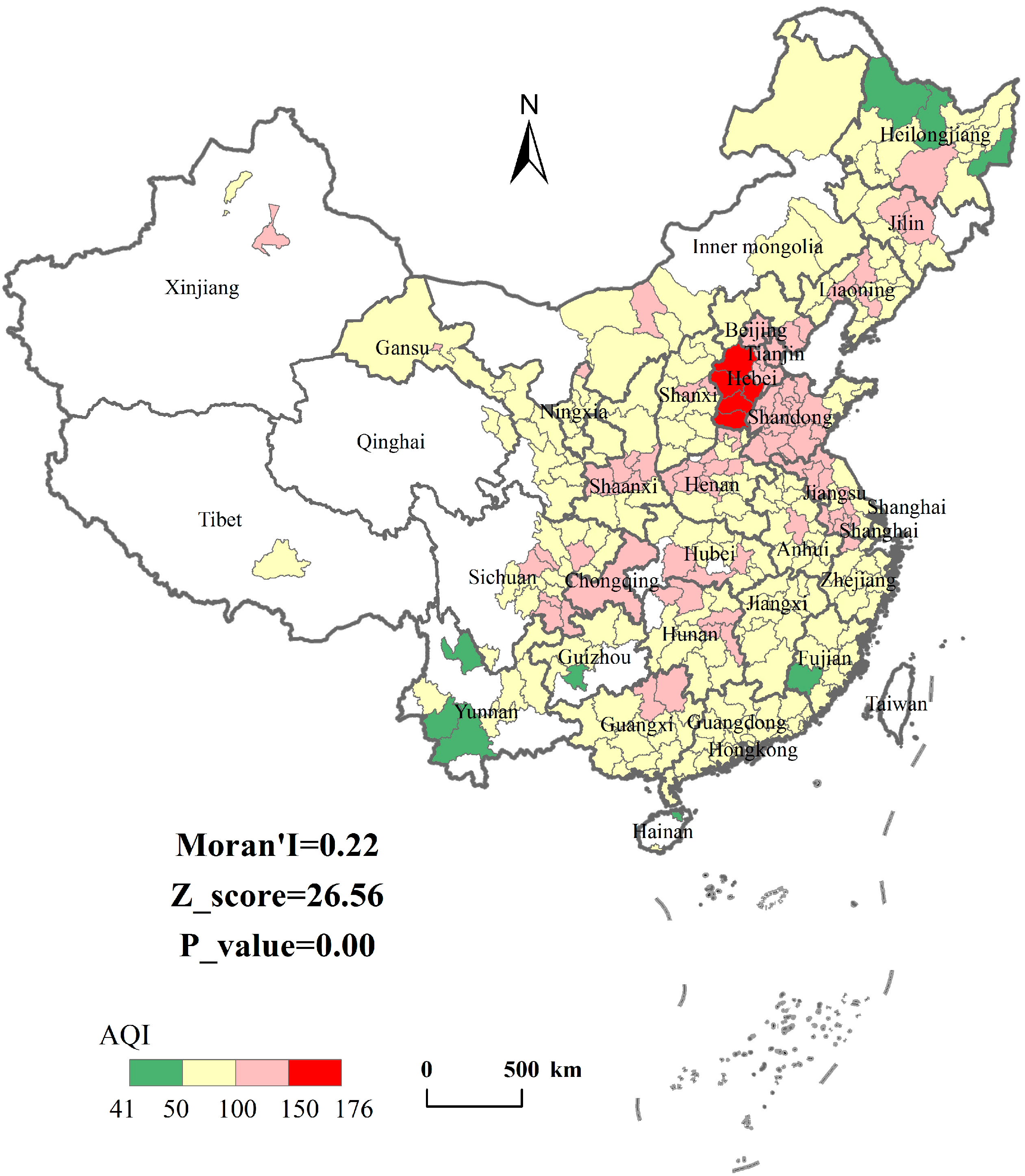
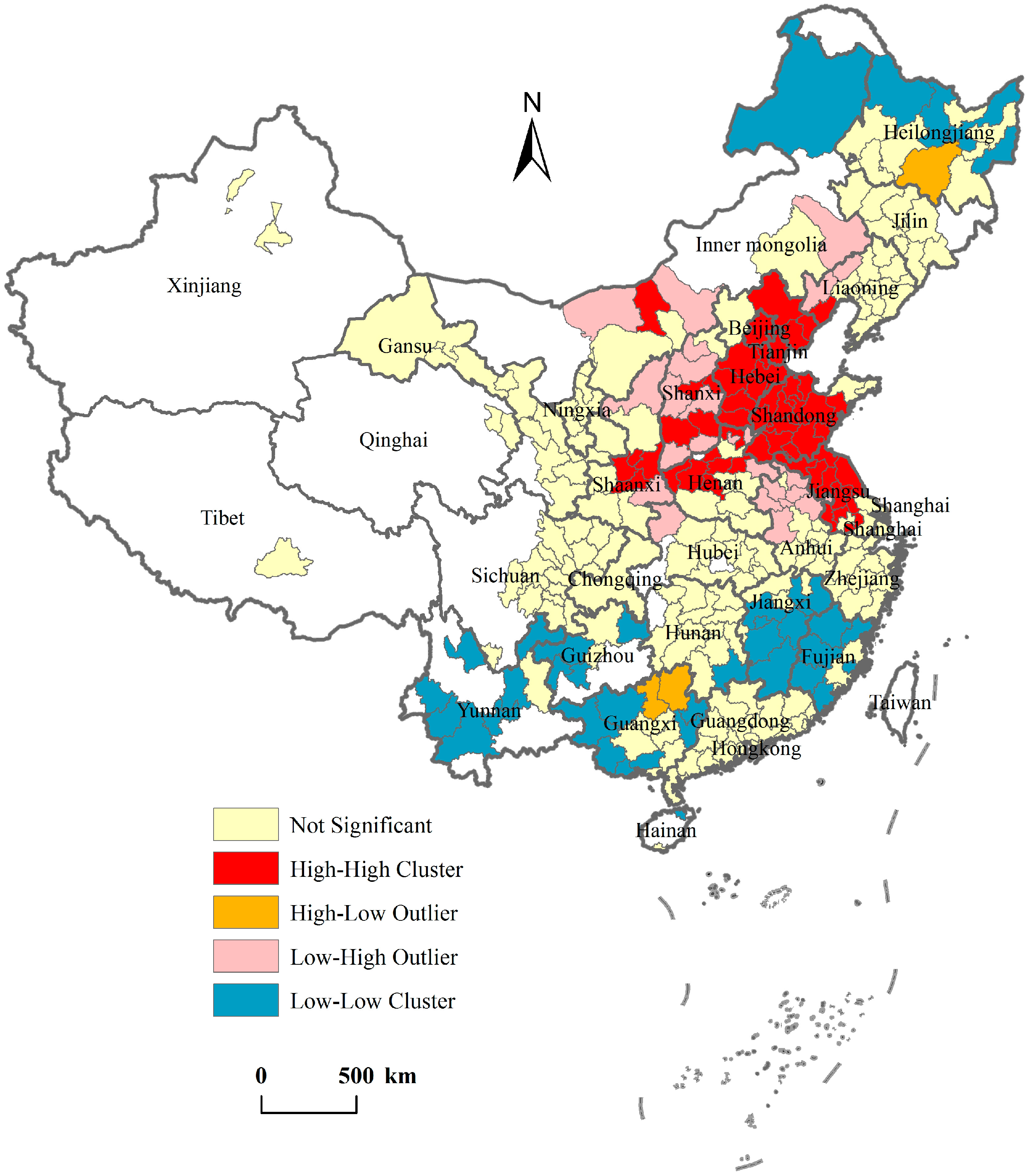
4.1. Spatial Pattern of AQI

Using the six grades that make up China’s AQI (good, moderate, unhealthy for sensitive groups, unhealthy, very unhealthy, and hazardous) as a basis (Table 1), considering the range of AQI value is 41.15–175.7, the spatial distribution of urban air quality in China’s 289 cities (285 prefecture-level cities and four municipalities) was divided into four levels (marked in four colors—green, yellow, pink, and red—in Figure 1). From the results of this study, as expressed in terms of this division, we can see very clearly that the AQI distribution displays definite spatial clustering characteristics. Of the 289 cities that were considered in this study, there were five cities that maintained an AQI value greater than 150 in 2014—these were all located in the Hebei province. The 72 cities with an AQI value of between 100 and 150 were mainly distributed across the North China Plain, within the Sichuan Basin, along the Longhai railway, and in parts of Northeast China. Most cities (70.24% of the total) were found to maintain an AQI value of between 50 and 100. It is regrettable that only nine cities reached the “Good” level (i.e., AQI < 50). In order to further explore the spatial autocorrelation of urban air quality, we built a spatial weight matrix that used inverse distance weighting (IDW), giving greater weight to points closer to the prediction location, and diminishing weight to points as a function of their distance from the prediction point. We subsequently used this matrix to calculate the global Moran’s I and local Moran’s I using Equations (4)–(6). The results returned a global Moran’s I of 0.22 and a Z-score of 26.56; the fact that the latter was greater than 2.58 (p = 0.01) suggests the existence of a significant and strongly positive spatial autocorrelation (a clustering of similar values) with respect to AQI values when analyzed at the city level.

The results of a LISA analysis, which measures spatial clustering and heterogeneity, are depicted visually at Figure 2. The specific cluster and outlier areas are also provided in this figure. Hot spot regions (H-H clusters) were found to include and surround the cities of Beijing, Tianjin, Hebei, Henan, and Shandong. Seriously polluted cities gathered closely together in these areas. Cool spot region (L-L cluster) were found to be located in three main areas: Heilongjiang, Yunnan-Guangxi, and the hilly areas of the southeast, suggesting that air quality was good in these cities and neighboring areas. Some outlier cities also formed L-H clusters. Overall, both the hot and cool spots indicate that the AQI values of Chinese cities exhibit both global spatial autocorrelation and also local spatial autocorrelation. As such, the data can be said to reflect spatial non-stationarity.

Figure 1. Spatial grade distribution and Moran’s I output of AQI.

Figure 1. Spatial grade distribution and Moran’s I output of AQI.

Figure 2. Clusters and outliers of AQI.

Figure 2. Clusters and outliers of AQI.

4.2. Estimation Results and Model Comparisons

The above analysis indicates significant spatial dependence in the AQI values of Chinese cities. In order to avoid model error and to improve the fitting precision, the spatiality of the factors studied should be taken into account. To compare to ordinary linear regression, we set up three global regression models using OLS, SAR, and SEM (Table 5). Through the OLS estimation, the R² (goodness of fit) of the model was found to be 0.338, the adjusted R² was 0.321, and the F-value was 20.484. The OLS model thus passed the significance test at the 1% level. The significance tests of the coefficients showed all the regression coefficients to be positive—that is to say, the selected explanatory variables were shown to all have a positive effect in relation to AQI values, a finding which was consistent with our expectations. Among the variables, TP, SI, and PD passed the significance test at the 1% level, meaning that these three urbanization factors exerted the greatest impact in relation to AQI. UR and PPC were also found to have significant influence in relation to AQI, clearing significance tests at the 5% level. Urban development land and per capita GDP, in contrast, failed the significance test at the 10% level. The diagnostic tests (i.e., Moran’s I, LM lag and LM error, p < 0.01) indicate clear problems with autocorrelation. Given this condition, the estimation results obtained from the OLS model may have led to biased parameter estimation, which in turn can cause problematic or even misleading conclusions.

Table 5. Ordinary least squares (OLS) estimation and spatial dependence.

Model	Coefficient	t-Statistic	Probability
constant	0.002	0.048	0.961
UR	0.171 **	2.447	0.015
TP	0.254 ***	3.246	0.001
UL	0.074	0.532	0.595
SI	0.163 ***	3.073	0.002
PD	0.302 ***	5.602	0.000
PGDP	0.045	0.584	0.559
PPC	0.129 **	2.291	0.023
R2	0.338
Adjusted R2	0.321
F-statistic	20.484
P(F-statistic)	0.000
AIC	715.992
Spatial Dependence	MI/DF	Value	Probability
Moran’s I (error)	0.056	7.016 ***	0.000
LM (lag)	1.000	42.059 ***	0.000
Robust LM (lag)	1.000	14.105 ***	0.001
LM (error)	1.000	28.963 ***	0.000
Robust LM (error)	1.000	1.009	0.315

Note: UR = The proportion of urban population; TP = Total population; UL = Urban development land; SI = Proportion of the added value of secondary industry to GDP; PD = Population density; PGDP = GDP per capita; PPC = Private cars per unit of urban development land; LM = Lagrange Multiplier; AIC = Akaike Information Criterion; ***, **, or * indicates significance at 1%, 5%, or 10% levels respectively.

Table 5. Ordinary least squares (OLS) estimation and spatial dependence.

Model	Coefficient	t-Statistic	Probability
constant	0.002	0.048	0.961
UR	0.171 **	2.447	0.015
TP	0.254 ***	3.246	0.001
UL	0.074	0.532	0.595
SI	0.163 ***	3.073	0.002
PD	0.302 ***	5.602	0.000
PGDP	0.045	0.584	0.559
PPC	0.129 **	2.291	0.023
R2	0.338
Adjusted R2	0.321
F-statistic	20.484
P(F-statistic)	0.000
AIC	715.992
Spatial Dependence	MI/DF	Value	Probability
Moran’s I (error)	0.056	7.016 ***	0.000
LM (lag)	1.000	42.059 ***	0.000
Robust LM (lag)	1.000	14.105 ***	0.001
LM (error)	1.000	28.963 ***	0.000
Robust LM (error)	1.000	1.009	0.315

Note: UR = The proportion of urban population; TP = Total population; UL = Urban development land; SI = Proportion of the added value of secondary industry to GDP; PD = Population density; PGDP = GDP per capita; PPC = Private cars per unit of urban development land; LM = Lagrange Multiplier; AIC = Akaike Information Criterion; ***, **, or * indicates significance at 1%, 5%, or 10% levels respectively.

The Lagrange Multiplier test, including LM (lag) and LM (error), passed the significance test at the 1% level, but the LM (lag) value was larger than latter. Meanwhile, the robust LM (lag) test was found to maintain significance at the 1% level, but the robust LM (error) failed the test of significance. Moreover, by comparing the goodness of fit of the SAR and SEM models—here, the R-square of SAR was found to be 0.390 and the R-square of the SEM was 0.374, and the AIC of the SAR was 700.132 and of the SEM was 703.372—and following the decision rule introduced above, the SAR model was considered the more appropriate model. Hence, we chose the SAR as the constant coefficient spatial regression model to study further.

Table 6 provides the detailed results of the GWR, OLS, and SAR estimation undertaken in this study. The AIC tests we conducted indicated the optimal bandwidth to be 857,196 m. The GWR model’s goodness-of-fit statistic was found to be much larger than that of either the OLS or the SAR models, and the GWR model was also found to have the lowest AIC value (36 points less than that of the OLS model and about 20 points less than that of the SAR model). Further, W_AQI was found to be 0.603 significant at the 1% level using the SAR model, that is to say: there existed an obvious spatial lag, meaning that the AQI value of a given city could be attributed not only to the influence factors of itself but, importantly, could be affected by the AQI values of neighboring cities. Compared to the OLS technique, SAR is more appropriate when dependent variables exhibit spatial autocorrelation. The GWR model performed the best of the three with respect to the issues addressed by this study.

Table 6. Parameter summary of geographically weighted regression (GWR), OLS, and spatial lag model (SAR) estimation.

Variables	Min.	Lower Quartile	Median	Mean	Global (OLS)	SAR (ML)	Upper Quartile	Max.
UR	−0.006	0.128	0.253	0.225	0.1708 **	0.171 **	0.336	0.381
TP	0.040	0.166	0.233	0.267	0.254 ***	0.246 ***	0.311	0.774
UL	−0.110	−0.069	−0.035	0.000	0.074	0.066	0.062	0.932
SI	0.067	0.112	0.133	0.132	0.163 ***	0.110 **	0.148	0.219
PD	0.186	0.239	0.259	0.273	0.302 ***	0.272 ***	0.296	0.497
PGDP	−0.212	0.019	0.075	0.087	0.045	0.037	0.143	0.257
PPC	−0.201	0.054	0.175	0.149	0.129 **	0.118 **	0.253	0.321
Intercept	−0.269	−0.075	0.091	0.053	0.002	−0.037	0.192	0.238
W_AQI				n.a.	n.a.	0.603 ***
No. of observations				289	289	289
Bandwidth				857196	n.a.	n.a.
R2				0.495	0.338	0.380
Adjusted R2				0.431	0.321	n.a.
AIC				679.866	715.992	700.132

Note: The Min., Max., Lower quartile, Upper quartile, Median, Mean are base statistics for the GWR model’s parameters. ***, **, or * indicates significant at 1%, 5%, or 10% levels respectively. UR = The proportion of urban population; TP = Total population; UL = Urban development land; SI = Proportion of the added value of secondary industry to GDP; PD = Population density; PGDP = GDP per capita; PPC = Private cars per unit of urban development land; AIC = Akaike Information Criterion.

Table 6. Parameter summary of geographically weighted regression (GWR), OLS, and spatial lag model (SAR) estimation.

Variables	Min.	Lower Quartile	Median	Mean	Global (OLS)	SAR (ML)	Upper Quartile	Max.
UR	−0.006	0.128	0.253	0.225	0.1708 **	0.171 **	0.336	0.381
TP	0.040	0.166	0.233	0.267	0.254 ***	0.246 ***	0.311	0.774
UL	−0.110	−0.069	−0.035	0.000	0.074	0.066	0.062	0.932
SI	0.067	0.112	0.133	0.132	0.163 ***	0.110 **	0.148	0.219
PD	0.186	0.239	0.259	0.273	0.302 ***	0.272 ***	0.296	0.497
PGDP	−0.212	0.019	0.075	0.087	0.045	0.037	0.143	0.257
PPC	−0.201	0.054	0.175	0.149	0.129 **	0.118 **	0.253	0.321
Intercept	−0.269	−0.075	0.091	0.053	0.002	−0.037	0.192	0.238
W_AQI				n.a.	n.a.	0.603 ***
No. of observations				289	289	289
Bandwidth				857196	n.a.	n.a.
R2				0.495	0.338	0.380
Adjusted R2				0.431	0.321	n.a.
AIC				679.866	715.992	700.132

Note: The Min., Max., Lower quartile, Upper quartile, Median, Mean are base statistics for the GWR model’s parameters. ***, **, or * indicates significant at 1%, 5%, or 10% levels respectively. UR = The proportion of urban population; TP = Total population; UL = Urban development land; SI = Proportion of the added value of secondary industry to GDP; PD = Population density; PGDP = GDP per capita; PPC = Private cars per unit of urban development land; AIC = Akaike Information Criterion.

Table 6 also presents base statistics for the models’ parameters across the entire sample of 289 cities. These include the minimum and the maximum values of GWR model’s parameters, as well as the values by quartiles. The OLS and SAR estimations are also listed for comparison purposes. On the whole, the value of the parameters estimated using OLS were higher than those obtained using SAR. If we take the mean value as the coefficient of the explanatory variables of the GWR model, the parameter estimations generated from all three models produced similar results: (1) Population density had the strongest effect on air quality, with this parameter being greater than 0.27 in all three models. Total population also proved to be significant, as the parameters for this variable were larger than 0.24; (2) At the 5% significance level, the parameters of urbanization rate and private car density reached 0.17 and 0.11 respectively; (3) per capita GDP and the area of urban development land, reflecting economic power and urban scale respectively, both failed to pass the significance test at 10%. Thus, we remain cautious about characterizing the relationship between the scale of urban land uses, economic conditions, and air quality. Finally, the parameter estimation of the proportion of secondary industry was different in each of the three models, reaching 0.163 at the 1% significance level with OLS model, while it was 0.11 significant at the 5% level in the SAR model, and had a mean of 0.132 in the GWR model.

Parallel coordinate plots of estimated GWR coefficients are visualizations that can be used for diagnosing correlation in estimated regression coefficients in typical, spatially varying coefficient model estimations [75]. As is shown in Figure 3, we took the intercept as the reference axis, with coefficients gradually getting larger, from the left to the right. One line represents one city, and the lines’ color changes from cool to warm in the axis so as to easily observe the parameters’ change of every city. The parallel coordinate plot at Figure 3 clearly shows correlation amongst the five groups of regression coefficients between different cities (for instance, there exists a strong consistency between the coefficients of the variables UR and PPC). It can also be observed that the distribution of the regression coefficients is unbalanced between the different axes. The coefficients of UR and SI are uniformly distributed in all cities, while the coefficients of TP and PD are centered in the low range for most cities. The results of GWR thus show that most of the regression coefficients spanned a wide range; with respect to their standard deviation, the minimum (SI) was 0.028 and the maximum (TP) reached 0.145. Wider ranges of variable parameters imply greater spatial variation in the contribution and explanatory effects in the model. To a large extent, the contribution of SI had no obvious spatial heterogeneity and dependence. Moreover, the regression coefficients of four explanatory variables in the GWR model in fact presented as negative values, with the minimum coefficient of PPC reaching −0.201. This further illustrates the appropriateness of the GWR model in providing a better explanation and more detailed results with respect to local estimation.

Figure 3. Parallel coordinate plot of the estimated GWR coefficients for intercept and five significant explanatory variables. Note: s.d. = standard deviation; UR = The proportion of urban population; TP = Total population; SI = Proportion of the added value of secondary industry to GDP; PD = Population density; PPC = Private cars per unit of urban development land.

Figure 3. Parallel coordinate plot of the estimated GWR coefficients for intercept and five significant explanatory variables. Note: s.d. = standard deviation; UR = The proportion of urban population; TP = Total population; SI = Proportion of the added value of secondary industry to GDP; PD = Population density; PPC = Private cars per unit of urban development land.

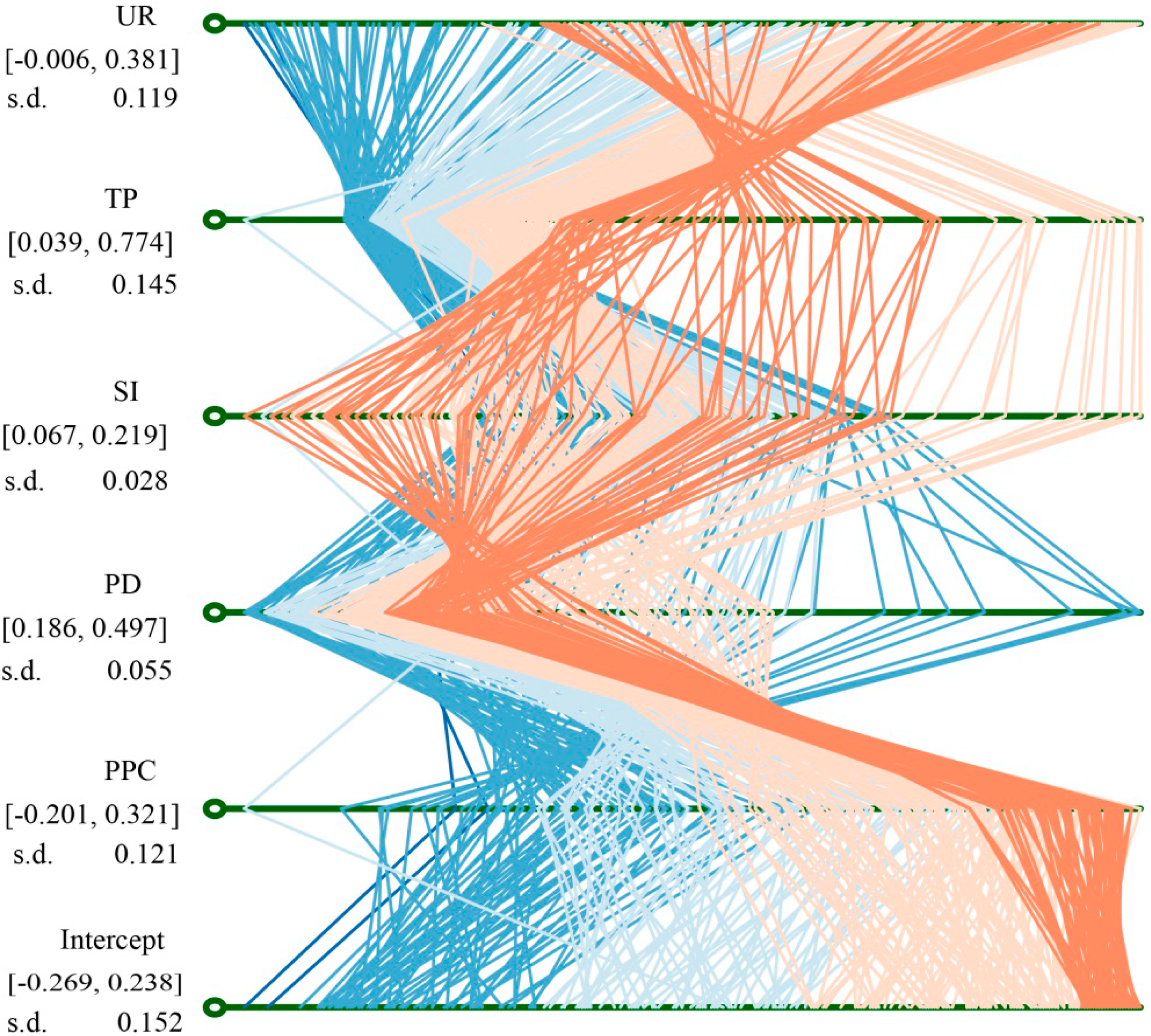
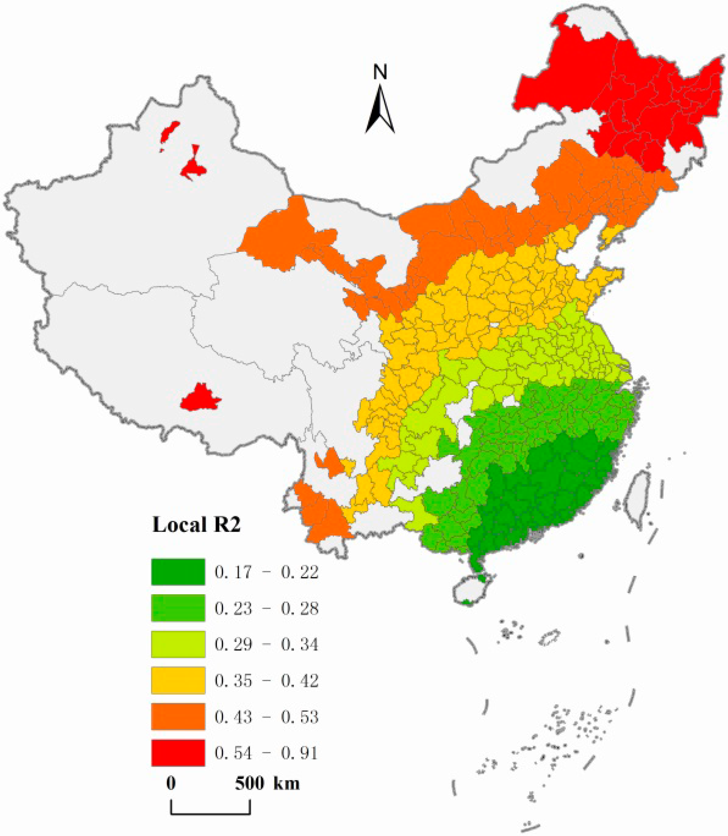
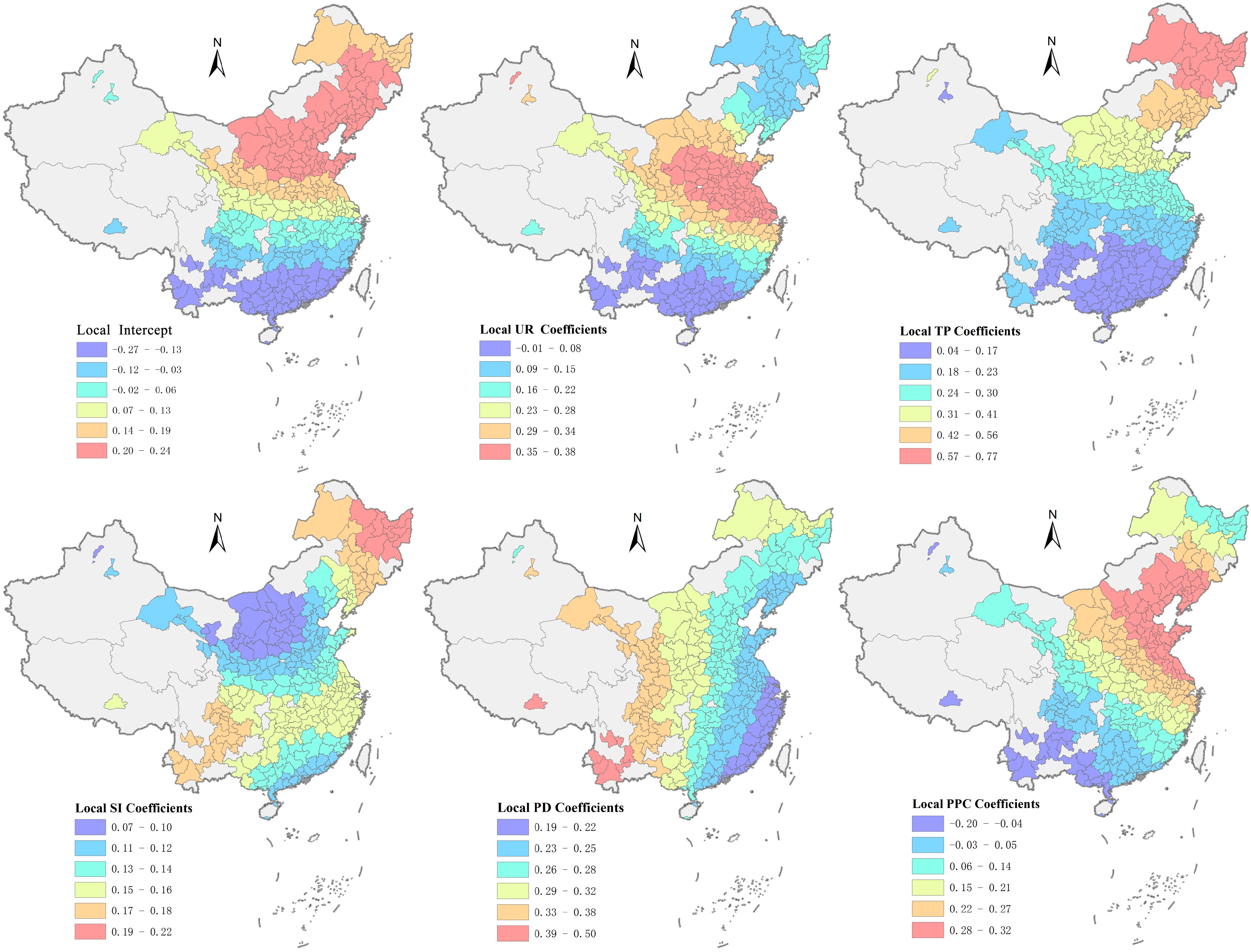
4.3. Spatial Distribution of GWR Estimation

The OLS model explains 33.8% of the variance of AQI values in Chinese cities, which is lower than the 49.5% obtained through GWR global R-Squared. In Figure 4, GWR local R-Squared values are mapped, yielding a number of interesting results. The local R-square was found to vary between 0.17 and 0.91 with the spatial variation, which means that some local models had a better fit than the OLS model, while some did not. Figure 4 demonstrates an obvious regularity in the spatial distribution of R-Squared: clearly, the northern and western region have higher R-square values. This illustrates that the relationships between various urbanization factors and air quality were much better captured by the regression model in the northern and western areas. AQI values in the southeast region may, in comparison, be rather more affected by other factors—for instance, temperature or vegetation fraction.

Figure 4. The spatial distribution of GWR Local R-Squared.

Figure 4. The spatial distribution of GWR Local R-Squared.

Figure 5 depicts the spatial distribution of intercept terms in relation to the five significant explanatory variables. In principle, the intercept term measures the fundamental level of AQI, excluding the effects of all factors on urbanization. We can see clearly that the intercept values increase gradually from the south to the north. This implies that, under the same urbanization factors, the air quality (measured in terms of AQI values) of cities in the southern region is better than of those located in the northern areas of China.

Figure 5. The spatial distribution of GWR local coefficients. Note: UR = The proportion of urban population; TP = Total population; SI = Proportion of the added value of secondary industry to GDP; PD = Population density; PPC = Private cars per unit of urban development land.

Figure 5. The spatial distribution of GWR local coefficients. Note: UR = The proportion of urban population; TP = Total population; SI = Proportion of the added value of secondary industry to GDP; PD = Population density; PPC = Private cars per unit of urban development land.

The relationships between the AQI values of Chinese cities and the coefficients of the five significant urbanization factors (as calculated in this study) displayed considerable spatial variability. It can be observed from the spatial distribution of UR coefficients that the central areas had greater coefficient estimates, the northeastern region maintained average coefficient estimates, and the southwestern region lower estimates. The proportion of urban population thus played a more important role in the North China Plain. The spatial pattern of PPC coefficients was similar to those of UR, and the traffic factor was found to have the most important effect on air quality in the Bohai Bay Rim area. Further, both UR and PPC had a negative effect on AQI in some southwestern Chinese cities, and this might be related to their limited social and economic development, which is related to the retention of a natural environment that has not been affected by urbanization trends. The spatial distribution of TP coefficients displayed a laddered distribution which varied with latitudinal zonality, i.e., highest (>0.42) in the north to lowest (<0.17) in the south. This indicates that the population size of cities in the north of China had a greater impact on their AQI values than in the cities of the south. What is interesting is that the spatial distribution of PD coefficients displayed a pattern of longitudinal zonality. The impact of population density on air quality in eastern coastal China was thus found to be lower than that in western cities, although the population density of the eastern cities was in fact higher. The spatial distribution of SI coefficients also demonstrated relatively higher values in the cities of the northeastern region and the Yangtze valley, compared to other areas, a result which can be attributed to the presence of more heavy industries in these cities. Further, whilst the proportion of secondary industry is very high in the areas that are shown in dark blue in Figure 5 (these coincide with the coal production base of China), the SI coefficients were in fact found to be lower than 0.1, a finding which implies that coal production does not exert large impacts in relation to AQI, even though coal consumption is the main source of many pollutants.

Overall, the relationships between air quality and urbanization factors were shown to be spatially non-stationary, and the spatial distribution pattern of each local parameter very different from the other, even though each parameter showed some zonal regularity. The local regression coefficients generated by the analysis also reveal that the explanation power of variable does not increase in strength in response to changes in the value of urbanization indicators.

5. Conclusions and Policy Implications

5.1. Conclusions

This study first analyzed the spatial pattern of air quality in 289 cities in China, based on Air Quality Index (AQI) records from 2014. Using OLS, SAR, and GWR models, we quantitatively estimated the impact of China’s urbanization processes on air quality, highlighting and exploring the spatial contribution made by a range of urbanization factors in relation to variations in AQI values. We found the AQI of 96.89% of the cities studied to be larger than 50 in 2014, subsequently identifying a significant and strongly positive spatial dependence and heterogeneity in AQI values at the city level. Seriously polluted cities were found to be gathered closely together in Beijing, Tianjin, Hebei, Henan, and Shandong, which presented as hot spots on the visualizations.

Regression models revealed that all the seven explanatory variables used to depict the urbanization process in fact exerted a negative effect in relation to air quality. The interpretation degree of the R² reached between 38% and 49.5%, confirming that, with the exclusion of natural factors, urbanization plays an important role in determining air quality. Among the variables, the population, urbanization rate, automobile density, and the proportion of secondary industry were all found to have had a significant influence over air quality. The area of urban development land and per capita GDP, in contrast, failed the significance test at 10% level although they maintained a remarkable correlation with AQI. The results of Moran’s I and SAR modeling indicated that the AQI value of a city can be attributed not only to influencing factors stemming from the city itself but also that of neighboring cities. The GWR results showed that the relationship of urbanization to air quality was not constant over space, but rather varied, with relations being more accurately captured by the regression model in the northern and western areas. The visualization of local parameter estimates highlighted the great spatial variation, which exists in the impact exerted by different urbanization factors in relation to different regional AQI values. These results also reinforce the complementary nature of these methods: the OLS (and SAR) results provided needed context for the GWR model, and the GWR was able to be used for simulating air quality in a manner that could take into account spatial dependence and heterogeneity.

In addition, these results should be generalized with caution, and it is emphasized that the present study only addresses the Chinese context. Whether the results of the study are suitable for other developing countries constitutes a matter for further examination. Considering the strong linkage exposed here between natural factors and air quality, it recognized that is also necessary to integrate natural and urbanization-related factors, and a comprehensive mechanism should thus be developed for such an operation through the future research.

5.2. Policy Implications

With the rate and scale of urbanization expected to drastically increase in the next 30 years, Chinese government officials face serious challenges in addressing the issue of air pollution. Through this paper, we propose several suggestions based on the empirical results:

Firstly, this study provides scientific validation for the presence of a strong spatial dependence in air quality at the city scale mainly because of the atmospheric flow. On the other hand, the pollutants are generated not only stationary sources (e.g., industry) but also non-stationary sources (e.g., vehicles). As such, we should take into full account spatial factors and policies must be directed at the source, increasing awareness of regional environmental systems. Air pollution prevention and control should be coordinated, with complementary measures undertaken across adjacent regions, especially in the urban agglomerations (e.g., Beijing-Tianjin-Hebei).

Secondly, because overall population density and total population play the most important roles in determining air quality, from the perspective of improving the country’s urban air quality, China must strictly control the scale of megacities and actively develop small and medium-sized cities. Automobile density and the proportion of secondary industry has significant impacts in relation to AQI values: thus, on the one hand, China must promote intelligent traffic management, increase the proportion of green public transport and reasonably controlling the vehicle population in order to reduce emissions from transport; on the other, more attention needs to be paid to accelerating the adjustment and transformation of the country’s industrial structure, accelerating the elimination of lagging productivity, and reducing dependence on coal.

Thirdly, we should fully acknowledge the spatial dependence and heterogeneity present in the relation between various parameters of urbanization and air quality in different geographic areas in China. Regional inequality between Chinese cities in terms of both urbanization and economic development is very large [76], and regionally specific policy analysis should be undertaken by local governments with respect to the various influence mechanisms exerted by urbanization on the atmospheric environment. The macroscopic environment policy of the central government should ultimately act to balance these regional differences on the basis of the understanding that “one size does not fit all”.

References

1. Chan, C.K.; Yao, X. Air pollution in mega cities in china. Atmos. Environ. 2008, 42, 1–42. [Google Scholar] [CrossRef]
2. Kan, H.; Chen, B.; Hong, C. Health impact of outdoor air pollution in china: Current knowledge and future research needs. Environ. Health Perspect. 2009. [Google Scholar] [CrossRef] [PubMed]
3. Matus, K.; Nam, K.-M.; Selin, N.E.; Lamsal, L.N.; Reilly, J.M.; Paltsev, S. Health damages from air pollution in China. Glob. Environ. Chang. 2012, 22, 55–66. [Google Scholar] [CrossRef]
4. Wong, E. Air Pollution Linked to 1.2 Million Premature Deaths in China. 2013. Available online: http://ming3d.com/sustainable/wp-content/uploads/2013/04/Air-Pollution-linked-to-Premature-Deaths.pdf (accessed on 18 November 2015).
5. Rohde, R.A.; Muller, R.A. Air pollution in China: Mapping of concentrations and sources. PLoS ONE 2015. [Google Scholar] [CrossRef] [PubMed]
6. Crane, K.; Mao, Z. Costs of Selected Policies to Address Air Pollution in China; RAND Corporation: Santa Monica, CA, USA, 2015. [Google Scholar]
7. Zhang, D.; Liu, J.; Li, B. Tackling air pollution in China—What do we learn from the great smog of 1950s in London. Sustainability 2014, 6, 5322–5338. [Google Scholar] [CrossRef]
8. Ma, T.; Zhou, C.; Pei, T.; Haynie, S.; Fan, J. Quantitative estimation of urbanization dynamics using time series of DMSP/OLS nighttime light data: A comparative case study from China’s cities. Remote Sens. Environ. 2012, 124, 99–107. [Google Scholar] [CrossRef]
9. Beirle, S.; Boersma, K.F.; Platt, U.; Lawrence, M.G.; Wagner, T. Megacity emissions and lifetimes of nitrogen oxides probed from space. Science 2011, 333, 1737–1739. [Google Scholar] [CrossRef] [PubMed]
10. Hopke, P.K.; Cohen, D.D.; Begum, B.A.; Biswas, S.K.; Ni, B.; Pandit, G.G.; Santoso, M.; Chung, Y.-S.; Davy, P.; Markwitz, A. Urban air quality in the Asian region. Sci. Total Environ. 2008, 404, 103–112. [Google Scholar] [CrossRef] [PubMed]
11. NBSC. China Statistical Yearbook 2014; China Statistics Press: Beijing, China, 2014. (In Chinese) [Google Scholar]
12. Grimm, N.B.; Faeth, S.H.; Golubiewski, N.E.; Redman, C.L.; Wu, J.G.; Bai, X.M.; Briggs, J.M. Global change and the ecology of cities. Science 2008, 319, 756–760. [Google Scholar] [CrossRef] [PubMed]
13. Fang, C.L.; Wang, J. A theoretical analysis of interactive coercing effects between urbanization and eco-environment. Chin. Geogr. Sci. 2013, 23, 147–162. [Google Scholar] [CrossRef]
14. Zhou, N.; Fridley, D.; Khanna, N.Z.; Ke, J.; McNeil, M.; Levine, M. China’s energy and emissions outlook to 2050: Perspectives from bottom-up energy end-use model. Energy Policy 2013, 53, 51–62. [Google Scholar] [CrossRef]
15. Liu, L.; He, P.; Zhang, B.; Bi, J. Red and green: Public perception and air quality information in urban China. Environ. Sci. Policy Sustain. Dev. 2012, 54, 44–49. [Google Scholar] [CrossRef]
16. Yuan, Y.; Liu, S.; Castro, R.; Pan, X. PM2.5 monitoring and mitigation in the cities of China. Environ. Sci. Technol. 2012, 46, 3627–3628. [Google Scholar] [CrossRef] [PubMed]
17. Chen, M.; Liu, W.; Lu, D. Challenges and the way forward in China’s new-type urbanization. Land Use Policy 2015, in press. [Google Scholar] [CrossRef]
18. Bai, X.; Shi, P.; Liu, Y. Society: Realizing China’s urban dream. Nature 2014, 509, 158–160. [Google Scholar] [CrossRef] [PubMed]
19. Molina, M.J.; Molina, L.T. Megacities and atmospheric pollution. J. Air Waste Manag. Assoc. 2004, 54, 644–680. [Google Scholar] [CrossRef] [PubMed]
20. Tai, A.P.; Mickley, L.J.; Jacob, D.J. Correlations between fine particulate matter (PM2.5) and meteorological variables in the United States: Implications for the sensitivity of PM2.5 to climate change. Atmos. Environ. 2010, 44, 3976–3984. [Google Scholar] [CrossRef]
21. Zhang, Z.; Zhang, X.; Gong, D.; Quan, W.; Zhao, X.; Ma, Z.; Kim, S.-J. Evolution of surface O3 and PM2.5 concentrations and their relationships with meteorological conditions over the last decade in Beijing. Atmos. Environ. 2015, 108, 67–75. [Google Scholar] [CrossRef]
22. Asimakopoulos, D.; Flocas, H.; Maggos, T.; Vasilakos, C. The role of meteorology on different sized aerosol fractions (PM10, PM2.5, PM2.5–10). Sci. Total Environ. 2012, 419, 124–135. [Google Scholar] [CrossRef] [PubMed]
23. Gebhart, K.A.; Kreidenweis, S.M.; Malm, W.C. Back-trajectory analyses of fine particulate matter measured at big bend national park in the historical database and the 1996 scoping study. Sci. Total Environ. 2001, 276, 185–204. [Google Scholar] [CrossRef]
24. Han, L.; Zhou, W.; Li, W.; Meshesha, D.T.; Li, L.; Zheng, M. Meteorological and urban landscape factors on severe air pollution in Beijing. J. Air Waste Manag. Assoc. 2015, 65, 782–787. [Google Scholar] [CrossRef] [PubMed]
25. Leibensperger, E.M.; Mickley, L.J.; Jacob, D.J. Sensitivity of us air quality to mid-latitude cyclone frequency and implications of 1980–2006 climate change. Atmos. Chem. Phys. 2008, 8, 7075–7086. [Google Scholar] [CrossRef]
26. Ramsey, N.R.; Klein, P.M.; Moore, B. The impact of meteorological parameters on urban air quality. Atmos. Environ. 2014, 86, 58–67. [Google Scholar] [CrossRef]
27. Zhang, Y.; Ding, A.; Mao, H.; Nie, W.; Zhou, D.; Liu, L.; Huang, X.; Fu, C. Impact of synoptic weather patterns and inter-decadal climate variability on air quality in the north China plain during 1980–2013. Atmos. Environ. 2015, in press. [Google Scholar] [CrossRef]
28. Hirota, K. Comparative studies on vehicle related policies for air pollution reduction in ten Asian countries. Sustainability 2010, 2, 145–162. [Google Scholar] [CrossRef]
29. Schmale, J.; von Schneidemesser, E.; Dörrie, A. An integrated assessment method for sustainable transport system planning in a middle sized German city. Sustainability 2015, 7, 1329–1354. [Google Scholar] [CrossRef]
30. Hao, J.; Wang, L. Improving urban air quality in China: Beijing case study. J. Air Waste Manag. Assoc. 2005, 55, 1298–1305. [Google Scholar] [CrossRef] [PubMed]
31. Jacobson, M.Z. Review of solutions to global warming, air pollution, and energy security. Energy Environ. Sci. 2009, 2, 148–173. [Google Scholar] [CrossRef]
32. De Leeuw, F.A.; Moussiopoulos, N.; Sahm, P.; Bartonova, A. Urban air quality in larger conurbations in the European Union. Environ. Model. Softw. 2001, 16, 399–414. [Google Scholar] [CrossRef]
33. Zhao, J.; Chen, S.; Wang, H.; Ren, Y.; Du, K.; Xu, W.; Zheng, H.; Jiang, B. Quantifying the impacts of socio-economic factors on air quality in Chinese cities from 2000 to 2009. Environ. Pollut. 2012, 167, 148–154. [Google Scholar] [CrossRef] [PubMed]
34. Ryu, Y.-H.; Baik, J.-J.; Lee, S.-H. Effects of anthropogenic heat on ozone air quality in a megacity. Atmos. Environ. 2013, 80, 20–30. [Google Scholar] [CrossRef]
35. Han, L.; Zhou, W.; Li, W.; Li, L. Impact of urbanization level on urban air quality: A case of fine particles (PM2.5) in Chinese cities. Environ. Pollut. 2014, 194, 163–170. [Google Scholar] [CrossRef] [PubMed]
36. Cho, H.-S.; Choi, M.J. Effects of compact urban development on air pollution: Empirical evidence from Korea. Sustainability 2014, 6, 5968–5982. [Google Scholar] [CrossRef]
37. Stone, B., Jr. Urban sprawl and air quality in large us cities. J. Environ. Manag. 2008, 86, 688–698. [Google Scholar] [CrossRef] [PubMed]
38. Xia, T.-Y.; Wang, J.; Song, K.; Da, L. Variations in air quality during rapid urbanization in Shanghai, China. Landsc. Ecol. Eng. 2011, 10, 181–190. [Google Scholar] [CrossRef]
39. Beelen, R.; Hoek, G.; Vienneau, D.; Eeftens, M.; Dimakopoulou, K.; Pedeli, X.; Tsai, M.-Y.; Künzli, N.; Schikowski, T.; Marcon, A. Development of no 2 and no x land use regression models for estimating air pollution exposure in 36 study areas in Europe–the escape project. Atmos. Environ. 2013, 72, 10–23. [Google Scholar] [CrossRef]
40. Borrego, C.; Martins, H.; Tchepel, O.; Salmim, L.; Monteiro, A.; Miranda, A.I. How urban structure can affect city sustainability from an air quality perspective. Environ. Model. Softw. 2006, 21, 461–467. [Google Scholar] [CrossRef]
41. Nowak, D.J.; Hirabayashi, S.; Bodine, A.; Greenfield, E. Tree and forest effects on air quality and human health in the United States. Environ. Pollut. 2014, 193, 119–129. [Google Scholar] [CrossRef] [PubMed]
42. Fang, C.; Liu, X. Temporal and spatial differences and imbalance of China’s urbanization development during 1950–2006. J. Geogr. Sci. 2009, 19, 719–732. [Google Scholar] [CrossRef]
43. The Daily Urban Air Quality. Available online: http://datacenter.mep.gov.cn/ (accessed on 18 November 2015).
44. World Health Organization. Air Quality Guidelines: Global Update 2005. 2006. Available online: http://www.euro.who.int/__data/assets/pdf_file/0005/78638/E90038.pdf (accessed on 18 November 2015).
45. Fang, M.; Chan, C.K.; Yao, X. Managing air quality in a rapidly developing nation: China. Atmos. Environ. 2009, 43, 79–86. [Google Scholar] [CrossRef]
46. NBSC. China City Statistical Yearbook 2014; China Statistics Press: Beijing, China, 2014. (In Chinese) [Google Scholar]
47. NBSC. China’s Regional Economic Statistical Yearbook 2014; China Statistics Press: Beijing, China, 2014. (In Chinese) [Google Scholar]
48. Biao, Q.; Chuanglin, F. The dynamic coupling model and its application of urbanization and eco-environment in Hexi corridor. J. Geogr. Sci. 2005, 15, 491–499. [Google Scholar] [CrossRef]
49. Li, Y.F.; Li, Y.; Zhou, Y.; Shi, Y.L.; Zhu, X.D. Investigation of a coupling model of coordination between urbanization and the environment. J. Environ. Manag. 2012, 98, 127–133. [Google Scholar] [CrossRef] [PubMed]
50. Akbari, H.; Pomerantz, M.; Taha, H. Cool surfaces and shade trees to reduce energy use and improve air quality in urban areas. Sol. Energy 2001, 70, 295–310. [Google Scholar] [CrossRef]
51. Xue, B.; Geng, Y.; Müller, K.; Lu, C.; Ren, W. Understanding the causality between carbon dioxide emission, fossil energy consumption and economic growth in developed countries: An empirical study. Sustainability 2014, 6, 1037–1045. [Google Scholar] [CrossRef]
52. Lozano, S.; Gutiérrez, E. Non-parametric frontier approach to modelling the relationships among population, gdp, energy consumption and CO2 emissions. Ecol. Econ. 2008, 66, 687–699. [Google Scholar] [CrossRef]
53. Mason, C.H.; Perreault, W.D., Jr. Collinearity, power, and interpretation of multiple regression analysis. J. Mark. Res. 1991, 28, 268–280. [Google Scholar] [CrossRef]
54. Dietz, T.; Rosa, E.A.; York, R. Environmentally efficient well-being: Is there a Kuznets curve? Appl. Geogr. 2012, 32, 21–28. [Google Scholar] [CrossRef]
55. Stern, D.I. The rise and fall of the environmental Kuznets curve. World Dev. 2004, 32, 1419–1439. [Google Scholar] [CrossRef]
56. Song, M.-L.; Zhang, W.; Wang, S.-H. Inflection point of environmental Kuznets curve in mainland China. Energy Policy 2013, 57, 14–20. [Google Scholar] [CrossRef]
57. Brajer, V.; Mead, R.W.; Xiao, F. Searching for an environmental Kuznets curve in China’s air pollution. China Econ. Rev. 2011, 22, 383–397. [Google Scholar] [CrossRef]
58. Anselin, L.; Rey, S.J. Perspectives on Spatial Data Analysis. 2010. Available online: http://link.springer.com/book/10.1007%2F978-3-642-01976-0 (accessed on 18 November 2015).
59. Tobler, W.R. A computer movie simulating urban growth in the Detroit region. Econ. Geogr. 1970, 46, 234–240. [Google Scholar] [CrossRef]
60. Tiefelsdorf, M. Modelling Spatial Processes: The Identification and Analysis of Spatial Relationships in Regression Residuals by Means of Moran’s I (Germany). Ph.D. Thesis, Wilfrid Laurier University, Waterloo and Brantford, ON, Canada, May 1998. [Google Scholar]
61. Anselin, L. Local indicators of spatial association-lisa. Geogr. Anal. 1995, 27, 93–115. [Google Scholar] [CrossRef]
62. Arribas-Bel, D.; Sanz-Gracia, F. The validity of the monocentric city model in a polycentric age: US metropolitan areas in 1990, 2000 and 2010. Urban Geogr. 2014, 35, 980–997. [Google Scholar] [CrossRef]
63. Zhang, C.; Luo, L.; Xu, W.; Ledwith, V. Use of local Moran’s I and GIS to identify pollution hotspots of Pb in urban soils of galway, ireland. Sci. Total Environ. 2008, 398, 212–221. [Google Scholar] [CrossRef] [PubMed]
64. Fischer, M.M.; Getis, A. Handbook of Applied Spatial Analysis: Software Tools, Methods and Applications; Springer Science & Business Media: Berlin, Germany, 2009. [Google Scholar]
65. Ali, K.; Partridge, M.D.; Olfert, M.R. Can geographically weighted regressions improve regional analysis and policy making? Int. Reg. Sci. Rev. 2007, 30, 300–329. [Google Scholar] [CrossRef]
66. Anselin, L.; Bera, A.K. Spatial dependence in linear regression models with an introduction to spatial econometrics. Stat. Textb. Monogr. 1998, 155, 237–290. [Google Scholar]
67. Kelejian, H.H.; Prucha, I.R. Specification and estimation of spatial autoregressive models with autoregressive and heteroskedastic disturbances. J. Econom. 2010, 157, 53–67. [Google Scholar] [CrossRef] [PubMed]
68. Fotheringham, A.S.; Brunsdon, C.; Charlton, M. Geographically Weighted Regression: The Analysis of Spatially Varying Relationships; John Wiley & Sons: Hoboken, NJ, USA, 2003. [Google Scholar]
69. Yu, D.-L. Spatially varying development mechanisms in the greater Beijing area: A geographically weighted regression investigation. Ann. Reg. Sci. 2006, 40, 173–190. [Google Scholar] [CrossRef]
70. Lo, C. Population estimation using geographically weighted regression. GIScience Remote Sens. 2008, 45, 131–148. [Google Scholar] [CrossRef]
71. Chang, H.-S.; Chen, T.-L. Decision making on allocating urban green spaces based upon spatially-varying relationships between urban green spaces and urban compaction degree. Sustainability 2015, 7, 13399–13415. [Google Scholar] [CrossRef]
72. Gao, J.; Li, S. Detecting spatially non-stationary and scale-dependent relationships between urban landscape fragmentation and related factors using geographically weighted regression. Appl. Geogr. 2011, 31, 292–302. [Google Scholar] [CrossRef]
73. Song, W.; Jia, H.; Huang, J.; Zhang, Y. A satellite-based geographically weighted regression model for regional PM 2.5 estimation over the Pearl River delta region in China. Remote Sens. Environ. 2014, 154, 1–7. [Google Scholar] [CrossRef]
74. Tu, J.; Xia, Z.G. Examining spatially varying relationships between land use and water quality using geographically weighted regression I: Model design and evaluation. Sci. Total Environ. 2008, 407, 358–378. [Google Scholar] [CrossRef] [PubMed]
75. Wheeler, D.C. Visualizing and diagnosing coefficients from geographically weighted regression models. In Geospatial Analysis and Modelling of Urban Structure and Dynamics; Springer Netherland: Heidelberg, Germany, 2010; pp. 415–436. [Google Scholar]
76. Li, G.; Fang, C. Analyzing the multi-mechanism of regional inequality in China. Ann. Reg. Sci. 2014, 52, 155–182. [Google Scholar] [CrossRef]