A Method to Evaluate the Stimulation of a Real World Field of View by Means of a Spectroradiometric Analysis

Abstract

Stimulation elicited by a real world field of view is related to the color, the intensity and the direction of the information reaching the eye: different spectral power distributions of light trigger different responses. An evaluation of the stimulation provided by the field of view can be performed by measuring the spectral radiance with a spectroradiometer and weighting this data with an efficiency curve. Different weights (physical, physiological and psychological) can lead to different analyses and consequently to different results. The proposed method allows an overall and simplified evaluation of the field of view based on spectral and luminance measures and a script that processes the luminous information. The final aim of this approach is to provide further information about the light stimulation reaching the retina and to supply a qualitative evaluation of the field of view, allowing to know how much stimulation is coming from a certain area within the visual field depending on the type of surface, basing on spectral and directional information. This approach can have practical implications, allowing technicians and designers to take into consideration the possible visual fields, in order to properly shape the features of stimulation throughout the day, hence following a field of view-based dynamic design.

1. Introduction

The artificial lighting of modern offices, where workers spend most of their day, provide a completely different radiometric and photometric information respect to natural daylight in terms of intensity, spectrum, illuminance and luminance levels, distribution within the visual field, time and prior history of exposition [1,2,3,4]. Such exposition somehow influences our body rhythms, psychological responses and performances [5,6,7,8,9], namely known as non-visual effects of light. An additional pathway to the visual one does exist in our body that concerns the light signal: the non-visual pathway goes from the eye to the hypothalamus in the brain, where is located the suprachiasmatic nucleus (SCN), the human peacemaker that regulates several body functions [10,11]. In particular, when stimulated from the light, the SCN sends to the pineal gland the input of inhibiting the melatonin production, which is secreted during the night and for this reason it is called the hormone of sleep. Many studies investigated the relationship between light and some hormonal secretions and suppression, whose results have been synthesized in [12], which states the principles for “healthy lighting”.

Human vision has been studied for centuries, leading to a deepened knowledge of the long-known human light receptors, cones and rods: the first ones work under quite high illuminance levels, allowing diurnal vision, codified by the Photopic Efficiency Function V(λ) [13,14,15], the second ones work at low illuminance levels, allowing night vision [16,17,18], codified by the Scotopic Efficiency Function [19]. Under intermediate conditions between photopic and scotopic view, there is the mesopic efficiency function, a recent object of study and recommendation [20].

Non-visual effects of light have only been investigated in the last decades: only in 2001 [21,22,23,24] a third photopigment, melanopsin, has been discovered inside a small population of retinal ganglion cells, the intrinsically photosensitive retinal ganglion cells (ipRGC): this opsin has been found to be directly related to the circadian system, which regulates our body rhythms. The spectral sensitivity of this system has not been definitively described yet [25], but its high sensitivity to short wavelength radiation around 460–480 nm and its very low sensitivity to wavelengths between 650 nm and 750 nm has been demonstrated, leading to a possible Circadian Efficiency Function, C(λ) [21,22,23,24,25,26,27].

Several scientific studies have been conducted by different research teams to describe the circadian sensitivity with an efficiency function, but they arrived to partial and not completely uniform results. Brainard et al. [21] and Thapan et al. [22], with independent empirical studies, established that the maximal sensitivity of the melatonin is about at 460 nm, but their different results for longer wavelengths led to two different efficiency curves; starting from these two works, several successive studies [26,28] elaborated other possible circadian efficiency functions, but none of them is still considered entirely descriptive of the non-visual response of human body. In the calculation the authors used the C(λ) function deriving from the results of Brainard et al. [21], as it is the most cited in literature, but it can be easily replaced with one of the curves developed in other researchers, of with a future most correct circadian efficiency function.

The capacity of different wavelengths to trigger non-visual responses is strictly associated to the irradiance level received at the eye [29], since it has been demonstrated that the effects on the circadian system are not due only to high irradiances, but they can intervene at normal intensity levels or even with dim light with a blue-enriched light [30], avoiding unwanted effects like glare. The first step to estimate the stimulation of the human body is to carefully characterize the radiation reaching the eye, as in terms of irradiance, as in terms in terms of spectral distribution, considering both the direct light and the reflections; then, it is necessary to apply to this complex stimulus the most correct circadian weighting function. The entrainment of the circadian system to the light/dark cycles is also dependent on the timing of exposure to the light sources: during night hours light suppresses the melatonin production, affects body temperature, hart rate and increases alertness, while light at morning can correctly reset the body functions. When the circadian system is not properly stimulated by light, either receiving too low light during the day or too much light during the night, circadian disruption could occurs: a misalignment between the biological and daily clock that can lead, in the short term, to jet-lag-like symptoms, and in the long term (for chronic misalignments) to more severe health issues, such as diabetes, a higher risk of developing cancer, and depression [31].

Although there is still a lot to learn about the impact of light on human health, the actual knowledge points out that the lighting of buildings and exterior spaces requires attention to this topic. As the circadian system and the non-visual responses are affected by both the intensity and the spectral composition of light, the environment can have a relevant influence on the light received by human eyes that has not to be underestimated. The light direct to the eye depends not only on the characteristic of the light source, in particular spectral power distribution (SPD) and intensities, but it is also affected by the physical features that characterize the environment; in the interiors, in addition to the typology of the artificial source, the presence of windows provides natural light sources, and their dimensions and orientation impact on its entity; moreover the surfaces, as in interiors as in exterior environments, reflect a percentage of light, depending on the color of the materials and even their consistence. All these are environmental variables that affect the quantity, intended as the irradiance level, and the quality of the light in terms of spectral composition reaching the eyes; even using the same light source, different environments, according with their specific features, can elicits different luminous stimulation for both the visual and non-visual systems. Several software available for lighting design allow reproducing the 3D model of interior or exterior settings and consider the environmental variables mentioned above in their algorithms; they are based on the vision function and are aimed to calculate photopic quantities, but no software calculates the non-visual stimulus. Till now only a mathematical formula has been developed to calculate the Circadian Light (CL) [28], but it takes into account only the direct effect coming from the light source and it does not consider the indirect components due to the environment.

In the traditional lighting design practice, the basic quantitative aspect of light is considered by standards [32] with regulations for the optimization of the energy efficiency [33] and the visual comfort within the environments. On the contrary, a specific standard about the quantification of non-visual effects of light, or suggestions and/or recommendations for obtaining the “circadian-based comfort” within an environment do not exist. In particular, the spectral composition as well as the intensity of the light reaching the eye, must be taken into account for quantifying its influence on the circadian system, so a specific methodology matching quantity and quality of light should be developed. Moreover, standards concerning visual performance usually refers to photopic quantities measured on the horizontal working surface, while the value to take into consideration for evaluating the non-visual effects of light is the vertical irradiance measured at the eye level.

So far, theoretical knowledge about this issue has not led to a quick and effective measurement protocol to evaluate circadian stimulation [26,28] elicited by a specific environment on human body, even if there is an urgent need of massive circadian screening of workplaces, for public health issues. Moreover, there is the need to take a step towards circadian friendly design, allowing an accurate circadian evaluation of a designed environment in a way that would make it possible, for architects and lighting designers, to make conscious design choices about light.

This work is aimed at implementing the capacity of evaluating the light stimulus, calculating the effect elicits by real settings on non-visual systems, which is applicable to the visual system too: the paper proposes a new methodology that considers as the direct component of light coming from the luminous sources, as well as the indirect components provided for reflection by the environment. A method for quantifying the stimulus provided by a real field of view, that integrates both the effect of the light intensity (quantitative effect) and the spectral composition (qualitative effect), is proposed by performing some simplifications and matrix calculations: this method is based on the assumptions that the visual field can be considered just as a tridimensional matrix, made up of points in the space, each one characterized by a luminance and a spectrum, whose effects on the visual system, as well as on the circadian system, can be calculated using the efficiency functions V(λ) and C(λ), respectively.

The circadian and the visual stimuli coming from a fixed point of view of an interior and an exterior environment are the results obtained with the application of this method. Two fields of view have been selected for having the basic feature of an interior and an exterior environment without presenting excessive complexities, so that they can be easily used for explaining and validating the proposed methodology; how to apply this method to more complex scenes is also indicated.

2. Materials and Methods

Current instrumentations perform radiometric and photometric measurements, quantifying singular quantities of the radiation physical phenomenon in the first case and of the luminous characterization in the second case; these instruments do not integrate in the same measure several quantities and do not consider the qualitative aspect with the quantitative one. The methodology presented in this work has the aim of quantifying at the same time the effect elicited by both the quantity, in terms of total irradiation, and the quality, as overall spectral composition, of the light radiation received by the eye; it calculates the whole luminous stimulation, both visual and non-visual, coming from a field of view, of an interior setting as well as of an exterior environment.

The method is based on the integration of measures performed in the real environment with post-processing by means of numerical calculation: measures of irradiance of the light source at the eye, reflectance of materials contained in the field of view and luminance of the scene are elaborated and their values are integrated in a numerical algorithm with the V(λ) or with the C(λ). Result of the calculation is a value representing, respectively, the visual or the circadian stimulus deriving from the field of view taken into account.

2.1. Simplifying Hypotheses

In order for the measurement and processing model to be valid, two simplifying hypotheses are necessary: the evaluation of a fixed field of view and the approximation of small areas within the visual field.

The method is based in the evaluation of static field of views, that are exemplified by shots performed with a digital camera, and for quantifying an environment that varies in time (as, for instance, a daylight scenario or a viewer’s change of direction of gaze), it would be required to analyze a series of shots, taken at different times. This operation can be performed more correctly with frames of a video when evaluating the visual stimuli, as the response of the visual system is immediate and the change in vision have to be monitored with a sequence of images taken in rapid succession. On the contrary the non-visual system has a slow adaptation time (minutes) to the change of lighting scenario, so the variation occurring in the field of view can be monitored with very large temporal steps; for this reason, in this second case, the fix point of view can be a valid approximation of the situation of an office, where the worker spends most of the hours at the desk in the same position.

The second hypothesis is linked to the fact that a common visual field is made up of many different objects, whose surfaces reflect light according to their spectral reflectance. For the purpose of the model, it is necessary to provide an acceptable approximation of the radiation reaching the eye: for this reason, only materials occupying an extended portion of the visual field are actually measured, while for the others only a rough approximation is performed as described at the end of the following paragraph.

2.2. Visual Field Examples

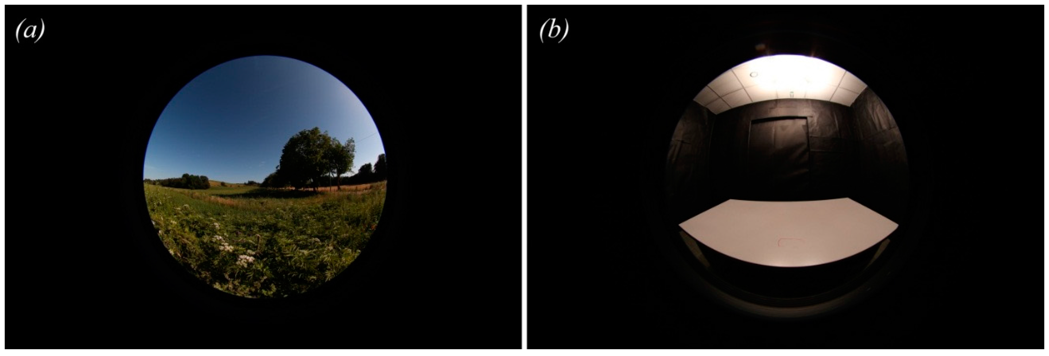
The numerical method for the evaluation of the luminous stimulus provided by the environment is based on a photo shot, as it is a valid approximation of the visual field: the spectral and the photometric quantities recorded at the eye were implemented in the algorithm. Two examples of visual fields are provided in Figure 1 for a better understanding and as experimental test of this method: an outdoor countryside view (V1), in which the field of view is divided in two main “materials”, the blue sky vault and the green grass on the ground, having very different luminance values and reflection coefficients; and an indoor controlled environment shot (V2), where the luminous stimulation comes mainly from the lamp and the only surfaces involved in reflection are the white ceiling and the light grey desk, being the lateral walls covered with a low reflective black material. The method employed for capturing the images is explained in the next Section 2.3.

A visual field is often made up of many different surfaces, some of which appear to occupy a very limited portion of it: considering the contribution of every single material can be impossible, or at least it can take quite too much time and effort for being considered a feasible method, hence it is necessary to choose and measure only the most extended materials, approximating the others. For the purposes of this method, a single material or a cluster of different materials occupying a little portion of the visual field have been approximated to one single material of the prevalent area, and associated, inside the calculation, to a material of a similar color, taken from a spectral reflectance library [34,35,36].

Figure 1. The two visual fields: (a) V1 divided by the blue sky in the upper part and the green grass in the bottom; and (b) V2 characterized by an artificial light source, the white ceiling, the grey desk and black walls.

Figure 1. The two visual fields: (a) V1 divided by the blue sky in the upper part and the green grass in the bottom; and (b) V2 characterized by an artificial light source, the white ceiling, the grey desk and black walls.

The error deriving from this approximation can be considered acceptable because it is used exclusively within small portion of the visual field; although this procedure can lead to a minimum degree of mistake because the human eye itself undergoes to an approximation due to metamerism, which is related to the fact that different spectral power distribution can result in the same perceived color. If, in a second moment, the need for a more precise analysis arises, because the image scene within the visual field is composed by many different objects of different colors, it is also possible to split the approximated area into smaller areas, and to associate each one of them a different material, allowing the technicians to reach the preferred level of approximation they need.

In the view V1, only the sky and the grass were taken into account, leaving out the trees on the background and in the V2 the black coating, the ceiling and the desk surface were considered, excluding the space under the desk, that indeed occupy a not-so small part of the visual field, but this was chosen only for didactical purpose.

2.3. Measurements

Measurements in the visual fields were recorded for calculating the stimulus, coming from the environment, received by the eye. The observed radiation corresponds to the radiance Lλ, which can be described as the irradiation Eλ coming from the light source that arrives on a surface and is reflected according to the reflectance Rλ of the surface; considering a Lambertian surface that reflects in all the direction of the hemisphere:

$$\text{Lλ}=\frac{\text{Eλ Rλ}}{\text{π}}$$

(1)

As this work proposes an experimental method, in this first attempt only Lambertian reflection for simplicity was considered, postponing the consideration of other typologies of reflection in future developments.

Multiplying Lλ with the V(λ) or with the C(λ), the visual (VS) and the circadian stimulus (CS) coming from the field of view can be respectively obtained:

$$\text{VS}={{\displaystyle \int }}^{\text{}}\text{LλV}\left(\text{λ}\right)\text{ dλ}$$

(2)

$$\text{CS}={{\displaystyle \int }}^{\text{}}\text{LλC}\left(\text{λ}\right)\text{ dλ}$$

(3)

Spectral radiance of the light source have been performed by means of a spectroradiometer Jeti Specbos 1211UV with a sensitivity of 1 nm, 10 degree observer, adaptive integration time, without additional lenses; it has been recorded at the eye level, corresponding to the visual fields V1 (Figure 2) and V2 (Figure 3).

Figure 2. Spectral radiance distribution of the natural light source measured at the eye in the V1: the emission was recorded in the bands of visible and UV-A, and it is characterized by high values in the low wavelengths and low values in the long wavelengths. The singular values for each wavelength were considered in the calculation procedure.

Figure 2. Spectral radiance distribution of the natural light source measured at the eye in the V1: the emission was recorded in the bands of visible and UV-A, and it is characterized by high values in the low wavelengths and low values in the long wavelengths. The singular values for each wavelength were considered in the calculation procedure.

The spectral reflectance of the materials was taken from on line libraries with free access [34,36].

Luminance measures were collected by simply taking a shot of the visual field, without any particular restriction by means a video luminance meter LMK Mobile Advanced based on Canon Eos 500D camera with a luminance calibrated 4.5 mm objective (fisheye); for performing luminance image measurements the instrument requests the following setting: focal aperture F4, autofocus, image stabilizer deactivated, auto exposure bracketing (AEB) ± 2 exposure values. The camera was mounted on a tripod at the eye height, considering a standing human in the V1 (170 cm) and a seated person in V2 (110 cm).

Each measurement was taken with the video luminance meter in the same direction as gaze (i.e., the same direction as the fisheye shot), and it was performed multiple times at different points, choosing the portions of material which appear to have the highest luminance; the mean values for each materials were then calculated inside a spreadsheet application.

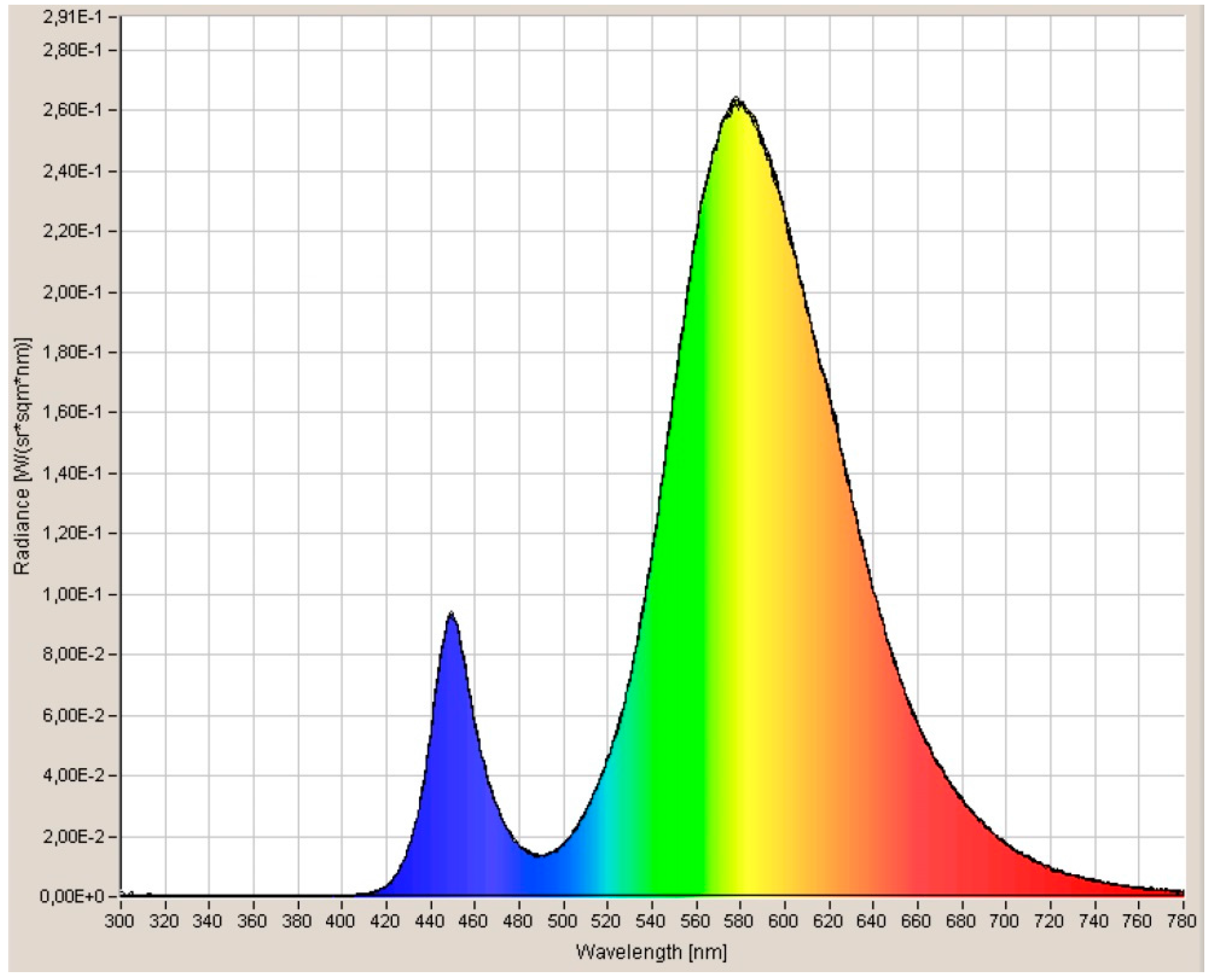
Figure 3. Spectral radiance distribution of the artificial light sources measured at the eye in the V2: the emission is limited to the visual field and it is characterized by a lower peak in the blue region and a higher peak in the yellow region. The singular values for each wavelength were considered in the calculation procedure.

Figure 3. Spectral radiance distribution of the artificial light sources measured at the eye in the V2: the emission is limited to the visual field and it is characterized by a lower peak in the blue region and a higher peak in the yellow region. The singular values for each wavelength were considered in the calculation procedure.

The instrument gives back two images representing the same field of view: a classical picture in jpg format and a pseudo-colors image with the corresponding luminance values in raw format; luminance values were extracted and processed inside LMK Labsoft software. Luminance image for the two examples of visual fields are reported in Figure 4.

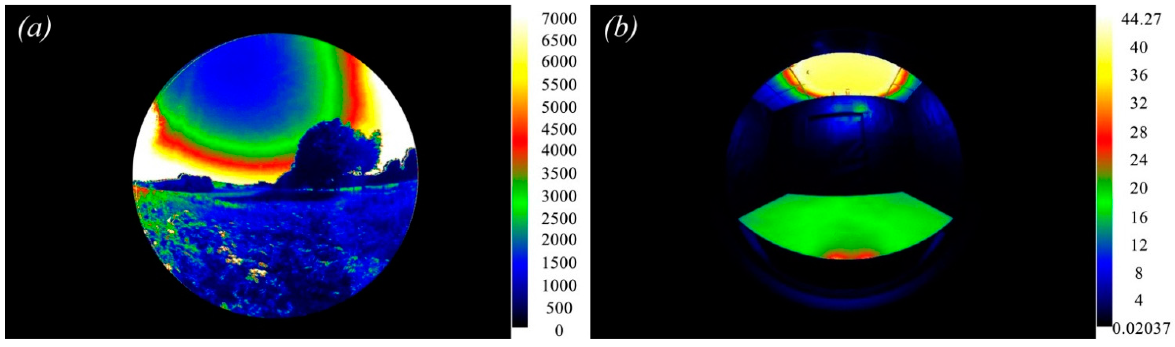
Figure 4. Luminance levels of V1 (a) and V2 (b) expressed in cd/m². In both the measures, the luminance coming from the bottom of the field of view has more constant values, than the luminance coming from the upper side. In the calculation procedure the singular value of each pixel was considered.

Figure 4. Luminance levels of V1 (a) and V2 (b) expressed in cd/m². In both the measures, the luminance coming from the bottom of the field of view has more constant values, than the luminance coming from the upper side. In the calculation procedure the singular value of each pixel was considered.

These spectral and photometric data were elaborated to obtain the stimulation deriving from the two fields of view taken into consideration.

As the stimulation deriving from the visual field is more complex than that coming from a single material, a procedure for applying the simplified model to the V1 and V2 has been performed: it made use of an elaboration of the images presented in Figure 1 and of an analytical calculation, as described in the next sections.

2.4. Reflectance-Material Coupling Procedure

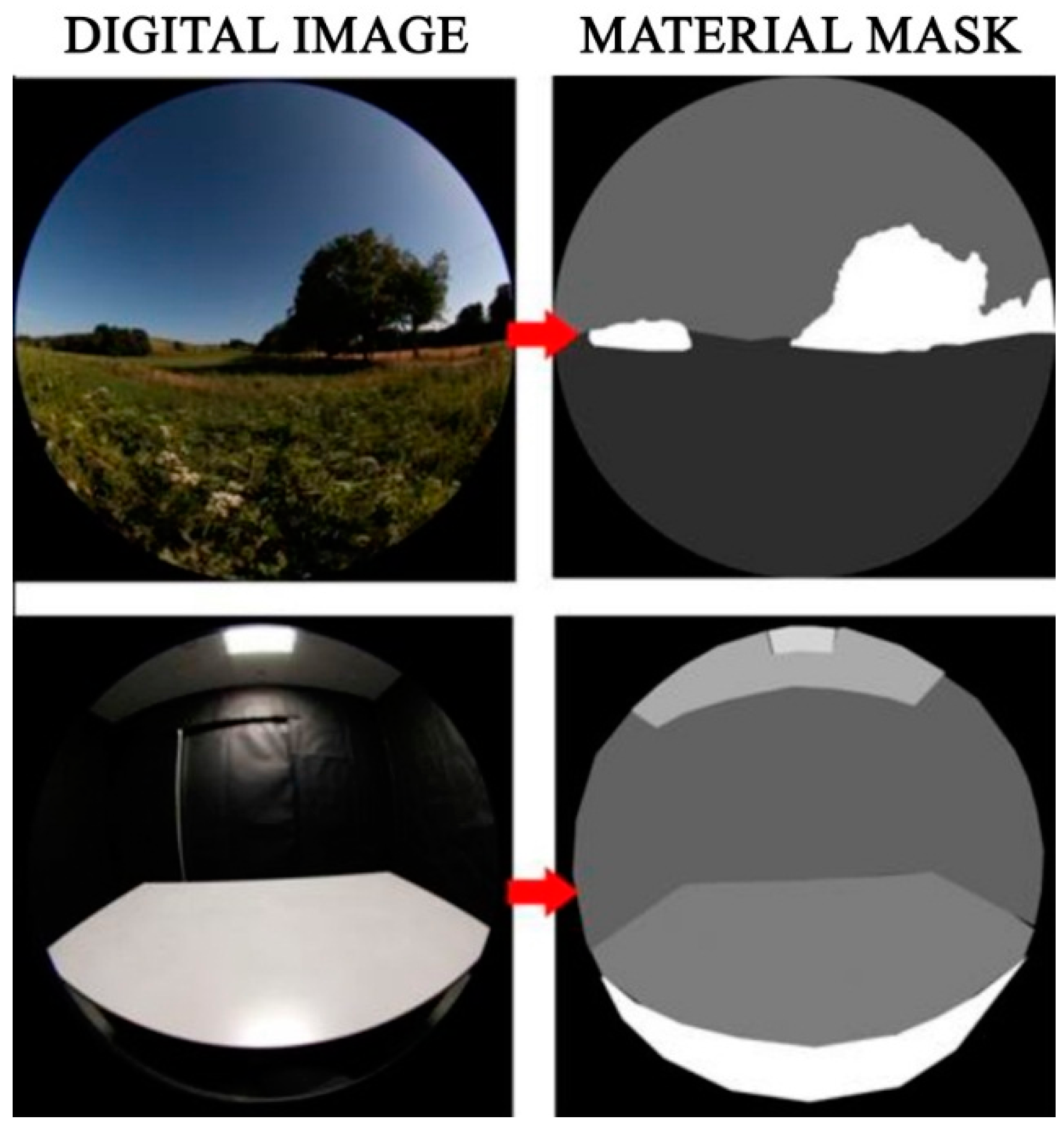
In order to associate every pixel of the image with its own spectral reflectance it was necessary to divide the visual field into heterogeneous zones, considering as the same part the homogeneous materials: visual field jpeg images were post-processed into an image editor, roughly drawing the contours of each material and filling each area with a different shade of gray. The output of this process is a grayscale jpeg, from now on called “material mask” made up of spots of different gray shades ranging between 0 (black) and 255 (white). The right column of Figure 5 shows material masks for the left column visual fields V1 and V2, and the areas corresponding to various materials are represented as different shades of gray (ranging from 0, corresponding to black, to 255, corresponding to white).

Figure 5. Digital images and corresponding rough material masks of the two visual fields: (up) in the outdoor picture the material masks were associated to three different areas corresponding to the sky, the grass and the trees; and (down) in the indoor picture the material masks were associated to five different areas corresponding to the light source, the ceiling, the walls, the desk and the space under the desk.

Figure 5. Digital images and corresponding rough material masks of the two visual fields: (up) in the outdoor picture the material masks were associated to three different areas corresponding to the sky, the grass and the trees; and (down) in the indoor picture the material masks were associated to five different areas corresponding to the light source, the ceiling, the walls, the desk and the space under the desk.

The lightness of the gray in the material mask does not respects the lightness of colors in the image, as the grayscale is only used for individuating the order in which the material will be successively processed: the material assigned to the darkest shade of gray will be the first one, while the material associated to the lightest shade of gray will be the last one. An example of grayscale subdivision for ten materials can be seen in Table 1.

Table 1. Example of convention between material numbers and grayscale values.

Material n #	1	2	3	4	5	6	7	8	9	10
Gray (0–255)	0	25	50	75	100	125	150	175	200	225

Table 1. Example of convention between material numbers and grayscale values.

Material n #	1	2	3	4	5	6	7	8	9	10
Gray (0–255)	0	25	50	75	100	125	150	175	200	225

Moreover, it is important that 0 is not used as a material filling, because the exterior part of the circular image of the field of view is already black (see Figure 2), and hence this color should be avoided in order to perform a valid calculation. This correspondence between the number codifying the material and the shade of gray its silhouette is filled with is necessary for the next step of the procedure. Furthermore, non-measured materials should be assigned to white mask (255), because they are processed in a second moment.

The example picture V1, representing a typical countryside view, was divided into three different material areas:

-

Area 1 corresponding to the grass, was associated to material 3 having a grayscale value of 50.

-

Area 2 corresponding to the sky, was assigned to material 4 having a value of 75 in the grayscale.

-

Area 3 corresponds to the trees; it was associated to the white mask (255 in grayscale value), as it was not measured.

The picture V2, representing a windowless indoor environment, was divided into five areas:

-

Area 1 corresponds to walls, is material 5 (100 in grayscale value).

-

Area 2 corresponds to the plasterboard ceiling, is material 6 (125 in grayscale value).

-

Area 3 corresponds to the desk surface, is material 7 (175 in grayscale value).

-

Area 4 corresponds to the LED luminaire, is material 8 (200 in grayscale value).

-

Area 5 corresponds to the floor tiles, which have not been measured, as because they occupy a little and peripheral portion of the visual field, as because their luminance is quite low; for this reason it is represented with the white material mask. In the study, the difference in light transmittance from the center and the periphery of the fisheye lens has not been investigated.

Each material mask image was considered a lines (n) per columns (m) two-dimensional matrix for processing.

2.5. Results: The Script

A script was written, for associating the pixels of the image, considered as an n × m matrix, to their relative values of spectral reflectance and luminance; it can be run by using spectral radiometric data from performed measurements, data coming from open databases of spectral reflectance and the luminance image.

In the script the spectral irradiance of the light source and the spectral reflectance of materials, acquired every 5 nm, can be seen as two column vectors with 81 values, while the luminance data are insert as image; photopic efficiency function V(λ) and circadian efficiency function C(λ) are both embedded in the code: in particular, since the latter has not been definitively established yet, it can be freely modified as soon as a better fitting function is developed.

The aim of this short code is to manage data, leading to a final radiance value coming from all the visual field.

The script performs the numbered steps described below.

(1) It asks the user to input the following data:

• Material mask (jpeg file, containing n × m × 1 values).
• Luminance image (txt file containing n × m × 1 values).
• Spectral reflectance of each one of the materials, uploaded in order (material 1 first, 81 × 1 values).
• Spectral irradiance of the light source (81 × 1 values).
• Number of measured materials within the scene (single value).

The program performs the following calculations.

(2) It counts the occurrences of every value inside the material mask and creates a two-column matrix that shows the values in column 1 and the number of their occurrences in column 2.

This step, together with 3 and 4, is performed because boundaries between different materials are affected by noise (values in the matrix different from the established ones of the grayscale), and thus it is necessary to remove such noise and obtain only the useful data out of the image.

(3) It sorts the values of the two-column matrix following the first column.

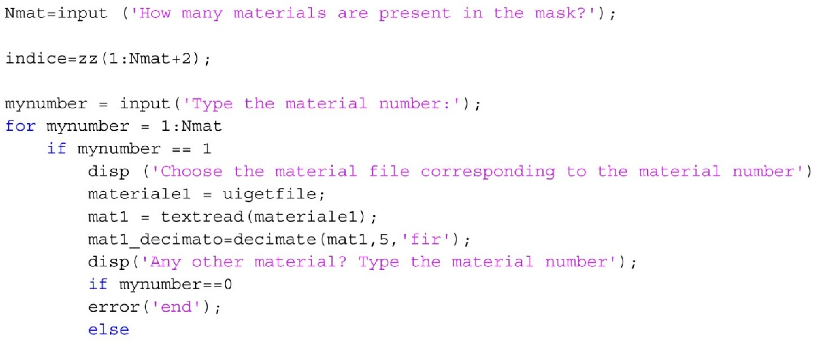
(4) It uses the number N of materials to extract the first n + 2 values with higher occurrence from the material mask (Figure 6). N + 2 is used in order to obtain the values in the material mask that correspond to the measured materials plus the two fixed values, that are 0 and 255, corresponding, respectively, to the outside of the visual field (black space around the fisheye image) and the non-measured materials, that are going to be approximated later on.

Figure 6. Script structure at point 4, used to extract the values with higher occurrence from the material mask.

Figure 6. Script structure at point 4, used to extract the values with higher occurrence from the material mask.

(5) It creates a three-dimensional matrix of zeroes with the same dimensions as the image and 81 sheets of depth (corresponding to the division of the visual field into a Δλ = 5 nm), attached behind the luminance image. This intermediate step is necessary because it is not possible to combine matrices whose dimensions do not match, but is mathematically possible to edit values inside a matrix that has the same n × m dimension as the image (Figure 7).

Figure 7. Script structure at point 5, which creates the three-dimensional matrix of zeroes.

Figure 7. Script structure at point 5, which creates the three-dimensional matrix of zeroes.

(6) It associates, to every single pixel in the image, its corresponding irradiance, weighted by the relative luminance value in that point. Such value, which is the ratio between the absolute luminance value in that position and the maximum luminance value of the image, is used as a correction factor in order to take into account different luminance of the same material within the scene, avoiding measuring irradiance of every single point. The theoretical basis on which this calculation is possible is the following: although luminance values are different in two points of the same material, and thus their spectral irradiance is different in absolute value, they do have anyway similar spectral distributions, only more flattened for lower luminance values.

(7) For each material, the spectral reflectance or the reflectance of the most similar color contained in the library is employed in the calculation.

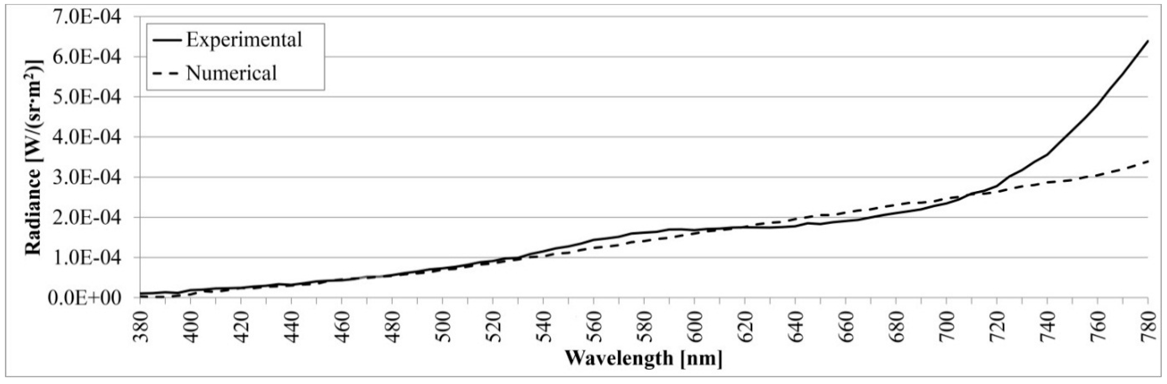
In a first attempt, the validation of the used analytical procedure was done using a simplified model that considered the stimulation coming from single materials: the difference between the value of radiance calculated through the formula 1 and the radiance measured was about 0.002 W/(sr·m²). The graph of Figure 8 shows the difference obtained in the spectral distribution with the material of the desk; the discrepancy occurred in the band between 720–780 nm is due to the spectral reflectance selected in the color library used in the calculation procedure, that presents small differences respect to real reflectance, as the color catalogued was very similar to that of the real material. The very small difference obtained in the final value of radiance validates the use of data contained into the libraries.

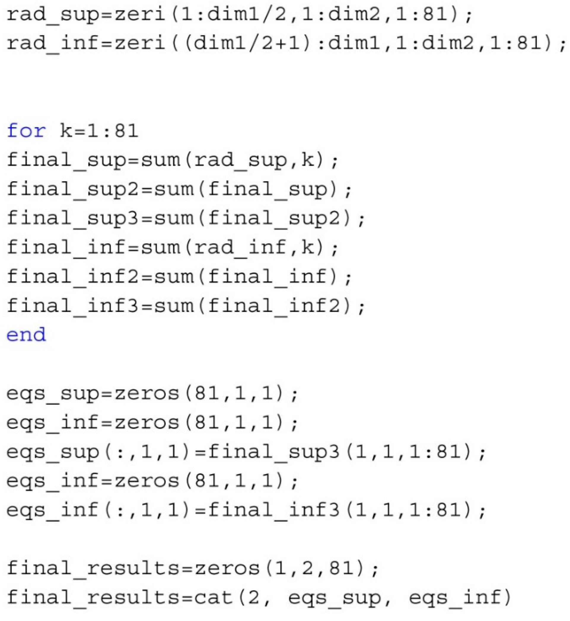
Figure 8. Example of procedure validation: obtained difference in the spectral distribution. The values of radiance calculated was very similar to the radiance measured in the most part of the visual spectrum, differing only in the long wavelengths between 720 and 780 nm (point 7). It calculates the average circadian radiance per wavelength of the all image using Equation (1) and outputs it in a table (Figure 9).

Figure 8. Example of procedure validation: obtained difference in the spectral distribution. The values of radiance calculated was very similar to the radiance measured in the most part of the visual spectrum, differing only in the long wavelengths between 720 and 780 nm (point 7). It calculates the average circadian radiance per wavelength of the all image using Equation (1) and outputs it in a table (Figure 9).

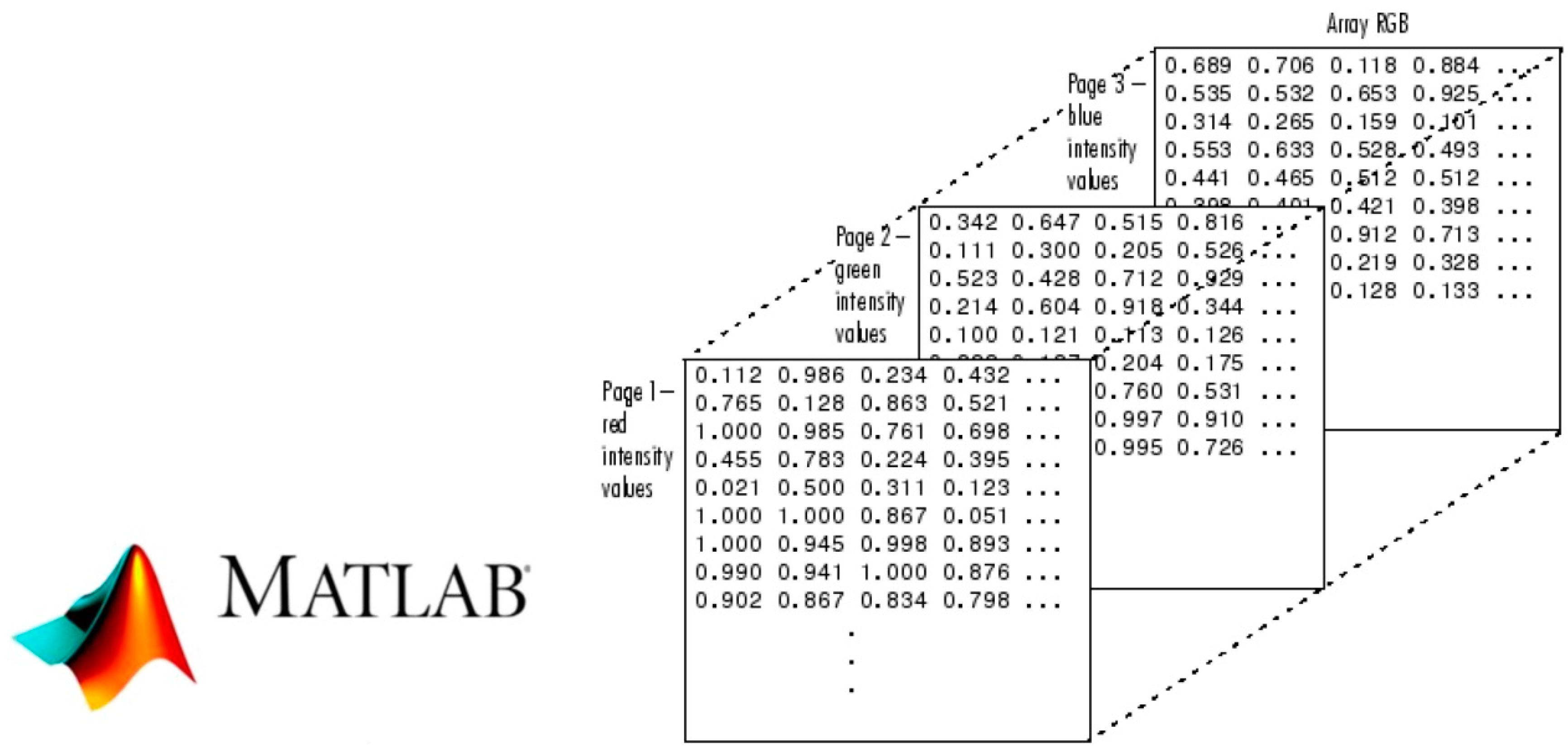
The final result is an n × m × 45 matrix (in the case of a 10-nm measurement) (Figure 10). In order to calculate the total irradiance reaching the eye for every wavelength, sums are performed: for those material whose reflection spectrum has not been measured because they occupied only a small portion of the field of view, the RGB values are considered.

Figure 9. Script structure at point 8 that calculates the average circadian radiance per wavelength.

Figure 9. Script structure at point 8 that calculates the average circadian radiance per wavelength.

Figure 10. Structure of a multidimensional n × m × 45 matrix to calculate the total irradiance reaching the eye for every wavelength.

Figure 10. Structure of a multidimensional n × m × 45 matrix to calculate the total irradiance reaching the eye for every wavelength.

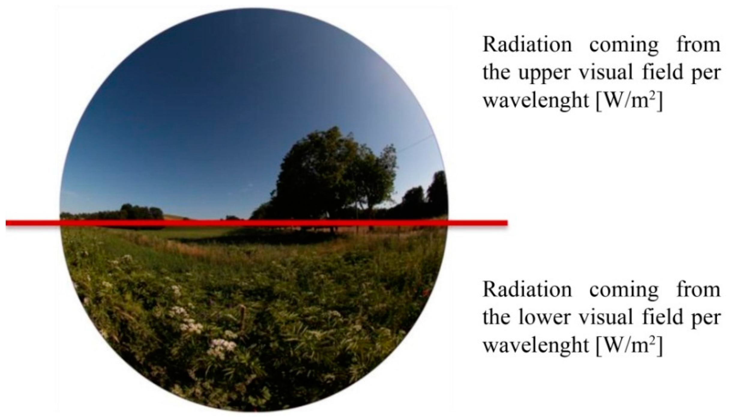
In this way, it is possible to know the quantity of light (radiance) per wavelength reaching the retina from different directions, allowing to distinguish between light coming from above the horizon and from below (Figure 11); for instance, within a room, the radiance coming from the light source and the windows located above and that reflected from the furniture located below the visual field can be measured independently. This operation is important for the calculation of the non-visual stimulus, as it has been discovered that the circadian photoreceptors, the ipRGC, are mainly placed in the inferior part of the retina, so they are principally stimulated from the light coming from the upper part of the visual field [37].

Figure 11. The method described allows knowing the radiation per wavelength reaching the eye and coming from the upper and from the lower half of visual field.

Figure 11. The method described allows knowing the radiation per wavelength reaching the eye and coming from the upper and from the lower half of visual field.

This numerical calculation can apply a circadian weighing function using Brainard’s circadian sensitivity function C(λ) to spectral reflectance of every material, hence obtaining what can be called “circadian reflectance”; then it performs a multiplication for each wavelength between circadian reflectance of each material and irradiance of the light source, resulting in circadian spectral irradiance of every material. However, spectral reflectance coefficient is non-dependent upon the light source lighting the material; hence, it is more useful in the case that data are collected by online resources.

3. Conclusions

The environment can have a relevant influence on the radiation received by human eyes, depending on the main features that characterize it; the typology of the source, the window dimensions, the color of the materials and even their consistence, all these are environmental variables that affect the quantity, intended as the irradiance level, and the quality of the light in terms of spectral composition reaching the eyes.

The aim of this paper was to provide a methodology to evaluate circadian stimulation caused by real environments, considering both the direct and the indirect components, and to be able to estimate radiance coming from specific surfaces within a given visual field. The numerical method developed integrates the quantitative and the qualitative effects of the lighting inputs deriving from the whole environment contained in the considered field of view.

Two real fields of view, one of an exterior and one of an interior environment, have been used for explaining the procedure of calculation. First validation of the method was performed considering the stimulation deriving from single materials: validation consisted in a comparison between measured values vs. numerical evaluated values of well-known metrics (radiances and irradiances). The very small difference (0.002 W/sr m²) obtained in the simplified calculation allowed extending the model to the two examples of field of view considered in the paper, for which every zone was studied intensely and every possible quantity was measured.

The confined environment comparison gave an error percentage in the range of 15%; this is a very good result, although we have to consider the extreme simplicity of the environment under examination, because of the number of simplifications introduced in the experimental procedure and in the calculation method that could determine a higher percentage. On the other side, we obtained a different error percentage for the open environment, approximately 30%, which we still evaluated as a good result if we consider the extreme variability of the sky vault and that we ignored the presence of the trees.

Once the model is thoroughly validated, it will possible to employ it for practical applications, with slight model modifications. A brief list of possible applications, with some considerations, is provided below.

By adding one or more “area masks”, created with the same method as the material mask, it is possible to only calculate mean irradiance value for that area: in this way it is possible to study how radiation reach the human eye: from which direction, with which spectrum, how total irradiance spectrum takes shape depending on the extension and reflectance properties of the environmental surfaces.

By modifying the model so that it weights spectral irradiance with V(λ) instead of C(λ), it is possible to obtain illuminance of each point of the scene. By employing radiance in place of irradiance and performing the previous modification, it is possible to obtain luminance.

It is also possible to extend the analysis to mesopic, scotopic or also biological efficiency function, leading to interesting compared analysis of the same visual field under different points of view.

The method described above is a two-way method, as it allows going both from real-world environment to circadian stimulation matrix, and back from digital rendering to circadian stimulation matrix.

The first way is described in this text, while for the second one, it is sufficient to have an RGB luminance (or illuminance) render made by one of the widespread lighting simulation tools, the spectrum of the light source chosen for the project and sample materials of the materials to measure under the light chosen.

Further research will be needed in order to solve critical points for this research. A numerical way of knowing which materials occupy a too small portion of the visual field to deserve being measured should be codified: it could be possible to implement such method using an image-recognition algorithm, which automatically recognize materials and calculates their area, but this falls out of the aim of the present research.