Global Sustainability Accounting—Developing EXIOBASE for Multi-Regional Footprint Analysis

Abstract

Measuring progress towards sustainable development requires appropriate frameworks and databases. The System of Environmental-Economic Accounts (SEEA) is undergoing continuous refinement with these objectives in mind. In SEEA, there is a need for databases to encompass the global dimension of societal metabolism. In this paper, we focus on the latest effort to construct a global multi-regional input−output database (EXIOBASE) with a focus on environmentally relevant activities. The database and its broader analytical framework allows for the as yet most detailed insight into the production-related impacts and “footprints” of our consumption. We explore the methods used to arrive at the database, and some key relationships extracted from the database.

1. Introduction

Perish or prosper? Human development must occur without overwhelming the natural ecosystems that we depend on. Sustainable development is now a constant focus of policy development, and sustainability metrics are becoming centralized within statistics. Models are continuously being developed to better inform policy processes while databases are being increasingly refined to provide the most complete and coherent description of society. To this end, focus has been applied on developing internationally applicable concepts within the United Nations framework for harmonizing economic and environmental accounting [1] so that we have global coverage and comparability between sustainability indicators. Significant progress has been made to harmonize the economic and environmental accounting principles with the System of Environmental-Economic Accounting (SEEA). We describe here the efforts made to operationalize a global-integrated accounting framework within the SEEA guidelines. The work focuses on the practicalities of implementing SEEA guidelines for data gathering, the amelioration of approaches for allocating supply chain impacts, and the demonstration of global impacts across the production and consumption perspectives. This paper focuses on the processes for arriving at such an integrated database within the concept of multi-regional (MR-) input-output (IO) analysis.

MRIO analysis is a rapidly developing field, and for a full review on databases and methodology we refer to Tukker and Dietzenbacher [2]. While regional IO analysis has been around for some time [3,4,5,6,7], its use in the calculation of global environmental footprints [8,9] and its relevance to climate policy issues, particularly with regard to carbon leakage [10,11,12,13], has significantly advanced the field’s development in the last decade. Currently, a considerable number of environmental and socio-economic issues that concern consumer behavior and that span global production networks use MRIO in order to fully account for demand-induced pressures [14,15,16,17,18,19,20].

This paper describes the preparation of harmonized multi-regional (MR-) monetary (M-) supply and use tables (SUT) including labor and environmental extensions for the year 2007. The paper gives insight into MRIO table compilation from preparation of source data to producing final MRSUT. For understanding of what is represented in an environmentally extended MRSUT, the reader is referred to Tukker et al. [15]. The work discussed here was developed within the auspices of EXIOBASE, a global multi-regional input−output database (see Section 1.2). In EXIOBASE, SUT are the basic building blocks from which a range of auxiliary data was used to create a harmonized and disaggregated MRSUT.

Through the use of MRIO frameworks, a significant amount of consistency is possible between the SEEA and resource accounting. We focus on those issues here, and conclude by providing a cursory insight into resource efficiency at the global level, and the links across the spectrum of pressure and impact categories and at macro- and mesoscales. The paper covers general ambitions in MRIO in the rest of Section 1, data in Section 2, followed by the methods employed within construction of EXIOBASE in Section 3. Some headline results are shown in Section 4 before conclusions and discussion of strengths and weaknesses occurs in Section 5.

1.1. Developments in Multi-Regional Input-Output Analysis (MRIO) Harmonization

In addition to the efforts to create EXIOBASE as described here, a number of other MRIO databases have been developed in recent years, most notably the World Input Output Database (WIOD) [21], Eora [22], Global Trade Analysis Project (GTAP) [23] and Organization for Economic Co-operation and Development (OECD) databases [24]. The different MRIO databases have been constructed with different foci for analysis; EXIOBASE has a clear environmental and resource focus with high levels of detail in primary production. All MRIOs, however, face similar issues in the harmonization of data and concepts. The following list describes general issues encountered in making a full MRIO as well as how these were specifically addressed in the case of EXIOBASE:

• Harmonizing and detailing supply and use tables (SUT)
  EXIOBASE has the objective to build a very detailed, multi-regional system of SUTs based on statistical data to the greatest extent possible.

  ○

  Gathering SUT from the relevant statistical offices. In the specific case of EXIOBASE, data is gathered from the EU27 via Eurostat, and other SUT and IO tables from 16 other countries. Together, these cover 90% of the global gross domestic product (GDP). (See supporting information for further details.)

  ○

  Harmonizing SUT to allow for consistency in pricing layers (treatment of margins and taxes), and for the consistent treatment of purchases by residents whilst abroad.

  ○

  Detailing SUT to give a consistent classification or, at a minimum, a link between classified imports and exports of different countries. This is either done through basic assumptions or, in the case of EXIOBASE, by using auxiliary data from FAO and European AgroSAM for agriculture, the International Energy Agency (IEA) database for energy carriers and electricity, various resource databases for resources, etc.

• Harmonizing and estimating environmental and social extensions
  The objective of EXIOBASE is to integrate a larger amount of data from environmental accounts, covering both resource inputs (energy, materials, water and land), as well as outputs of waste and emissions to air and water.

  ○

  Collecting and allocating available labor, material, land and water extraction data (e.g., the statistical databases of the Food and Agriculture Organization of the United Nations (FAOSTAT, Aquastat) and of the International Labor Organization (LABORSTA)) to product groups and industry sectors.

  ○

  Estimating energy and emissions data; in EXIOBASE, this involved transforming the energy data of the IEA database for 63 energy carriers from territory to residence principle and allocating the energy supply and use to sectors and final use categories. Emissions are estimated consistently for all countries on the basis of energy and other activity data and TNO’s bottom-up TEAM model [25].

• Linking the country SUT via trade
  With EXIOBASE, we aim to provide a fully trade-linked SUT system readily available for users to perform footprint-type assessments.

  ○

  Harmonizing UN Comtrade bilateral trade data with that of trade data of the SUT, whilst ensuring trade is symmetrical (matching) between importer and exporter.

  ○

  Splitting import use tables and allocating imports to countries of exports using harmonized trade data.

• Creation of MRIO tables and footprint analysis

In addition to the MRSUT, EXIOBASE also contains symmetric MRIO tables under various assumptions (in order for footprints or consumption-based accounts to be calculated, assumptions must be made on converting multiple output industries into single output activities, and further on linear demand-supply relationships [26]).

1.2. EXIOBASE Advances

The second version of EXIOBASE (EXIOBASE2—for the base year 2007) follows on from the first development of EXIOBASE (v1—for the year 2000 within the EXIOPOL project) [15], see Table 1. EXIOBASE2 sought to make advances compared to existing MRIO databases in a number of areas. Due to aggregation errors inherent to IO modeling [27], a focus was placed on increasing the product and industry detail of the model. To harmonize with the material balances of waste accounts derived elsewhere in the CREEA project, additional detail was put into both the product and industry classifications, resulting in 200 products and 163 industries (see supporting information) for enabling the tracing of waste and recycling flows. In addition to the sector detail, EXIOBASE2 estimated five additional “rest of world” regions for countries not explicitly covered in EXIOBASE v1. These changes make EXIOBASE2 the most detailed MRIO currently available. Adopted alongside the increased detail was rectangular instead of square SUT. This detail has been suggested to be essential for resource accounting [20]. This adoption provides the ability to represent a single technology that produces multiple co-products, such as an oil refinery.

Table 1. Developments of EXIOBASE [28].

Project	Database	Base Year	Available	Products/ Industries	Regions	References
EXIOPOL	EXIOBASE v1	2000	2012	129/129	44	Tukker et al. 2009 [29]; Tukker et al. 2012 [15]; Wood et al. [30]
CREEA	EXIOBASE v2	2007	2014	200/163	48	This paper; Tukker et al. 2014 [31,32]
DESIRE	EXIOBASE v3	1995–2014	2015	200/163	49	Under development [33]

Table 1. Developments of EXIOBASE [28].

Project	Database	Base Year	Available	Products/ Industries	Regions	References
EXIOPOL	EXIOBASE v1	2000	2012	129/129	44	Tukker et al. 2009 [29]; Tukker et al. 2012 [15]; Wood et al. [30]
CREEA	EXIOBASE v2	2007	2014	200/163	48	This paper; Tukker et al. 2014 [31,32]
DESIRE	EXIOBASE v3	1995–2014	2015	200/163	49	Under development [33]

The final main advancement of EXIOBASE2 was the expansion of monetary SUT to link to an additional physical SUT layer. The result is to express in the physical layer all product flows in mass (dry weight) or energy units, hence allowing for physical allocation. This implies that from a product perspective, the mass balance as well as the economic balance principle of “supply equals use” will hold, while also maintaining balances from an industry perspective (i.e., the supply of products by industry and outputs to nature are equal to the use of products and inputs from nature). The full physical layer was exploratory, and a comprehensive description of the approach to physical layering, and the outcomes of the layering, is beyond the scope of this paper (see [34]). Estimates of the physical layer and pricing estimates are available upon request, but results presented in this work are not based on them.

General Framework of Methods

Within industrial ecology and sustainability assessment in general, various methods stand out for the accounting of the social metabolism [35]. The three most prominent of these are (economy-wide) material and energy flow accounting, life cycle assessment, and IO analysis. All three methods attempt to model the complexity of production and consumption systems in order to trace source impacts to a functional demand. All methods share a similar methodological background [36], and significant scope is available for the integration of both data and methods [37].

EXIOBASE2 seeks to integrate economy-wide material and energy flow accounting with MRIO modeling (see [38,39,40]). This integration allows for the calculation of the various material flow metrics by recording used and unused extraction in each domestic economy, physical imports and exports, and enabling the tracing of raw material equivalents of imports and exports through Leontief modeling.

Life cycle assessment approaches are integrated through the use of life cycle inventory data to link the direct physical and monetary inputs required for the production of one unit of output in each industry sector, and by including characterization of environmental flows. At the basic level, the coefficients of the individual country IO tables were first estimated in both physical and monetary terms, linked by price estimates of the product groups and industry sectors. Hence, in this work, by using a consistent mathematical structure, all types of analysis from product life-cycle assessments to environmental footprints and economy-wide flow accounting can be performed.

2. Data Sources

A number of disparate databases were integrated in EXIOBASE2, thereby establishing consistency between the thematic areas covered by the databases whilst also facilitating inter-disciplinary modeling.

2.1. National Account (SUT) Data

The statistical national accounts in the form of SUT for the 43 countries and in the form of national account aggregates for the “rest of world” regions are used as the main building blocks. SUT form the basis of GDP calculations [41], ensuring consistency through the integrated database to national account aggregates. However, some adjustments are necessary. The first stage in using the SUT requires assembling the inventory and validation of original aggregate SUT data. Inventorying implies gathering:

• For EU27: ESA95 tables discerning 59 sectors and products
• For the 16 non-EU countries: SUT and/or IO table in different kinds of classifications

SUT data are not always consistent across countries and therefore need adjustment for the MRIO context. Tables occasionally report negative supply or negative sales when all values should be gross, and published tables are not always balanced. Hence, as a first stage of the data harmonization, concordances of classification are prepared and cursory data validation performed. Through a programmed interface, the data consistency is checked and errors in original tables are corrected. Harmonization across different accounting conventions is done in this step. Key aspects include the treatment of financial intermediation services indirectly measured (FISIM), the handling of purchases by residents abroad and of purchases on domestic territory by non-residents, the conversion or estimation of data to enable the estimation of basic price tables (price harmonization), the preliminary balancing of tables, and the re-basing of tables to a common base year. This automated approach creates datasets for multiple years and facilitates future data updates.

2.2. Trade

The main trade data used in EXIOBASE2 originates from the UN Comtrade database [42] and the UN services trade database [43]. The UN Comtrade data, although of reasonably high quality, is not symmetrical; bilateral exports are not consistent with the mirror country’s bilateral imports. The BACI database [44] is based on UN Comtrade, but is reconciled such that for a single year, every trade flow is recorded as a single bilateral trade flow in both physical units and in free-on-board (f.o.b.) monetary valuation.

2.3. Agriculture Social Accounting Matrices for European Countries (AgroSAM)

A set of social accounting matrices (SAM) for the EU27 was developed as part of the AgroSAM project at the Institute for Prospective Technological Studies [45]. These tables follow the standard Eurostat format for SUT in purchaser prices, but are extended to include feedbacks of primary inputs into final demand, although this feature is not used in this project. In addition, the project provided disaggregated agricultural data for 30 primary agricultural sectors and 11 food processing sectors. Such detail allowed the direct mapping of the AgroSAM database to the EXIOBASE2 classification for all sectors with the exception of fish product processing, which was aggregated with “food products nec”. As the AgroSAM data are only from 2000, the relative values (structure) of inputs and sales were taken for the agricultural and food sectors, and applied as coefficients for the disaggregation of the 2007 tables.

2.4. FAOSTAT and Other Sector Outputs

The Food and Agriculture Organization of the United Nations (FAO) database, FAOSTAT [46], provided in 2007 dollars, was used to estimate agricultural sector production values. These output data were coupled with the AgroSAM-derived coefficients for EU countries and the coefficient data for non-EU countries. Some adjustments were made to FAOSTAT data where there was a discrepancy between physical and monetary reported values.

Data for manufacturing product output for European countries are obtained from the PRODCOM database [47], and industry turnover from the Structural Business Statistics [48].

2.5. International Energy Agency Energy Balances

The International Energy Agency (IEA) Energy Balances database was used as the source of disaggregation for the energy flows [49,50]. The IEA database is converted from the territory to the residence principle based on the accounting rules provided by the United Nations Department of Economic and Social Affairs [51] and Eurostat [52] by applying auxiliary datasets [53]. The most important of these transformations occurs in the transport sector, where a transformation is needed from the place where fuels are sold (basis for the territory principle) to the use by residents of a country. A secondary step tailors energy supply and use and emission factors to the EXIOBASE2 industry and product classifications, i.e., translates IEA flow and product to existing EXIOBASE2 categories. Several auxiliary datasets were used to perform this transformation [53]. In addition, for use of the energy accounts in detailing monetary SUT, derived prices were applied.

2.6. Emission Accounts

Combustion-related air emission accounts are calculated directly on the basis of the energy accounts described above, providing implicit internal consistency between the energy and emission accounts [53]. To do so, the energy flows related to combustion are identified and combined with emission factors following the so-called energy-first approach described in Eurostat [54]. These emission factors for greenhouse gases and air pollutants are available from the guidance for estimating emissions of greenhouse gases and air pollutants at the national level. The Intergovernmental Panel on Climate Change (IPCC) Guidelines for National Greenhouse Gas Inventories [55] and the European Monitoring and Evaluation Programme/European Environment Agency (EMEP/EEA) Guidebook [56] for air pollutants provide the methodologies for emission estimation. This set of methodologies also forms the basis on which countries estimate their annual emissions under the United Nations Framework Convention on Climate Change (UNFCCC) and Convention on Long-Range Transboundary Air Pollution (CLRTAP) international conventions.

For each country and sector, a suitable methodology has been selected based on the importance of the source (a more important emission source requires a more detailed method) but also on data availability. The methods are applied to each sector and each country at the global level, resulting in a global emissions dataset. This dataset is compared to the official emissions to identify outliers and possible errors, which are corrected where needed. A one-to-one comparison is not possible because of the territory principle applied in the official country inventories.

For the non-combustion air emission accounts, emissions are calculated in a similar way by combining various activity statistics (e.g., industrial production, use of products) with the methodologies from the guidelines described above. The activity statistics have been collected from various data sources, including the material use database described earlier. Emission factors are taken from the guidance documents and applied to selected activity data for each sector. Similar to the combustion emissions, the non-combustion emissions are also compared to official UNFCCC and CLRTAP emissions to identify possible outliers and errors, but a detailed comparison was not possible due to the different basis (territory vs. residency principle).

2.7. Labor Accounts

Available labor statistics show the global distribution of work conditions from the point of view of where it occurs, both regionally and in main economic activities. Primary sources for labor inputs were national labor force surveys, gathered from the International Labour Organization’s (ILO) LABORSTA database [57], and a combination of labor force and industrial surveys in national accounts, obtained from the Organisation for Economic Co-operation and Development’s (OECD) STAN database [58]. Labor data from LABORSTA consist of 39 economic sectors, whereas STAN covers up to 60 industries and thereby provides better resolution compared to the MRIO sectors. Labor data were collected for labor according to skill level and gender, which allows for the calculation of further quality of labor indicators such as forced labor, child labor, vulnerable employment and damage-related indicators of labor through occupational health damage see Simas et al. [18,19].

2.8. Water Accounts

EXIOBASE is a comprehensive database with a high level of sector disaggregation. In contrast, the available data on water use and consumption collected by national statistical agencies, for example, are not of sufficient coverage or quality to fit the requirements of EXIOBASE—or simply altogether non-existent. As a consequence, modeled data covering the following categories were used. In the following, we describe the sectors for which data were used with regard to the type of water (blue/green) and the type of water flow (use/consumption). “Blue water” refers to water abstracted from surface water and groundwater bodies, whereas “green water” refers to water from precipitation, which infiltrates into the soil and is taken up by plants. “Water use” is the amount of water abstracted from water sources, whereas “water consumption” in the hydrological sense is the difference between the water abstracted and the water returned to the same watershed/ecosystem. In hydrological accounting terms, water consumption is defined as water evapotranspiration plus water incorporated into products [59].

• Agricultural water consumption (blue/green)
• Industrial water use and consumption (blue)
• Domestic water use and consumption (blue)
• Agricultural nitrogen and phosphorous emissions to water
• Thermal pollution of (heat emissions to) water from energy production

This last item addressing thermal discharges to water is a new quality aspect thus far unaddressed by the SEEA.

This data allows coverage of both water quality issues and emissions to water, thus permitting water use to be linked to actual environmental impacts [59]. Collection, classification and disaggregation of the water data were required before use. These steps were of special relevance in the case of industrial water use/consumption, wherein data from the WaterGAP model were used [60]. In contrast to the data on agricultural water appropriation, these data are not available in the full product detail, but for only five manufacturing sectors, two energy-producing sectors of different types of cooling systems (once-through vs. tower cooling), as well as for different types of livestock breeding. Hence, these data had to be allocated to the different product (and industry) groups used in EXIOBASE2. While this was a relatively straightforward task in the case of the livestock data, the data on water appropriation in the manufacturing sector had to be allocated to the more detailed EXIOBASE2 product classes using physical production quantity data for the different products. In the case of energy production, the data were allocated to the energy types that use cooling water in their production systems. Next, the data were allocated to the specific EXIOBASE2 sectors via the monetary data from the SUTs on sectorial activities [59].

2.9. Material Accounts

Data for the material extensions were retrieved from the Sustainable Europe Research Institute (SERI) Global Material Flow database [61]. The Global Material Flow Database is the only database with global coverage that comprises comprehensive resource extraction data for all material categories in annual time series. The database is organized according to the standards of economy-wide material flow accounting (MFA) as provided by Eurostat and the OECD [62,63].

The data in the Global Material Flow Database are mainly based on four data sources: the British Geological Survey (BGS) and the US Geological Survey (USGS) for metal and mineral data; the International Energy Agency (IEA) for the data on fossil fuels; and the Food and Agriculture Organization of the United Nations (FAO) for the data on biomass extraction.

2.10. Land Accounts

Cropland data are collected on the individual crop basis (primary crop classification in FAOSTAT), and supplemented by categories not commonly reported in statistics such as fallow land, forestry plantations on arable land and land for other agricultural purposes (see [64] for full details on land use data). In addition to the FAO online database, data and information were taken from a multitude of single, specific sources as documented in the detailed report found in the supporting information for this study. Also, Eurostat data for the aggregate categories “forage plants” and “fallow land” were taken from the agricultural database to fill data gaps or replace FAO data.

FAO data for primary crops inherit specific properties, including the double or multiple counts of land use in the case of multiple cropping in the span of one year. Such cropping practices are only counted once in the EXIOBASE2 extensions.

In addition to cropland, permanent meadows and pastures constitute the remainder of utilized agricultural land, and FAO reports permanent meadows and pastures as a single number. Forest area is a single number in FAO statistics comprising both natural forests as well as managed forests and plantations. Only the total area is reported; the statistics do not distinguish between the forest categories.

Built-up and related land encompasses all developed land, including transport corridors and human settlements. The base data for the category are the 2011 Annex 1 Party Greenhouse Gas (GHG) Inventory Submissions under the UNFCCC. Since these data do not cover all EXIOBASE2 countries and are not complete for some regions, we used additional single-country sources or international data such as from the European Corine Land Cover project.

3. Methods

MRIO table estimation generally requires the harmonization of the concepts in the above types of datasets, irrespective of the final database. However, there is also considerable variation in foci of methods across the MRIO databases currently available [2], which has implications for the amount of data reconciliation that needs to be undertaken. In the WIOD database, focus was placed on temporal and national account consistency, with more applications in socio-economic indicators [21] than most other MRIO databases. As such, aggregation of products and industries was a reasonable method to obtain high-level consistency between databases. A second approach is epitomized by Lenzen et al. [22], who seek a highly automated low-cost method to create the Eora MRIO database. This method, after an initial time investment required to estimate a snapshot of global economic structure, uses statistical information directly, with a single-stage mathematical reconciliation. EXIOBASE2 has more detailed product groups that allow an increase in precision with which environmentally relevant flows can be modelled through supply chains. As a result, attempts were made to reconcile data with particular attention paid to accurately describing (and disaggregating) the volume and structure of environmentally relevant activities. As such, after adjustment for convention, particular focus is applied in EXIOBASE2 to the tractability of the monetary and physical coefficient data, which form the backbone of the database and are reconciled to the various auxiliary data sources. As all auxiliary data are in the form of absolute flows, the coefficients must be transformed via estimates of disaggregated product and industry totals into disaggregated estimates of supply and use flow matrices before the data reconciliation takes place.

3.1. Disaggregating Product and Industry Totals

Because of the different classifications of individual countries, and because of the differences in data availability for each country, product and industry totals were generated in the EXIOBASE2 classification for each country that split aggregate SUT product/industry totals based on as much auxiliary data as possible.

A recursive routine added detail to the aggregate classification such that aggregate data were split group by group into sub-groups by adding more detailed data until the final classification is reached. This was particularly important for harmonizing data sources relating to services and the electricity sector, where non-electricity generation activities in the utilities sector needed to be split before the structure of the electricity generation of each country was estimated. Industry total disaggregation is performed using the same method as per product total disaggregation. Where industry-specific data are not available, product totals are used to calculate shares for disaggregating the industry totals.

3.2. Generation of Generic Coefficients

A set of generic coefficients form the underlying structure of the MRIO model, constructed in the final classification of EXIOBASE2. The coefficients represent the expected technology adopted in each industry, such as value of bauxite needed to produce one unit value of aluminum, and are used only to give the base structure of the disaggregate SUTs. Both supply and use coefficients are generated in order to capture the occurrences of by-production and joint-production. The generic use coefficients are first estimated based on product-by-product tables, before market share information from the supply coefficients is integrated to obtain country-specific use coefficients (Section 3.3).

The source of the generic coefficients is a combination of physical input per unit output data obtained from life cycle inventory databases, the most disaggregated IO tables available, and a “world average” mix of coefficients for poorly represented sectors [65]. Particular attention is given to collecting specific coefficient data for the electricity sectors, energy products, and agricultural products.

Physical coefficients for some agriculture, some energy and some manufacturing flows were taken from the work on physical SUT (physical input coefficients multiplied by prices). Additional detail was included for the electricity sector using GEM-E3 [66], for the aluminum sector using industry data [67], and for natural and manufactured gas from the detailed Australian SUTs (Australian Bureau of Statistics 2012). The summary of the most disaggregated IO tables used in the generic coefficients is given in Table 2.

Table 2. IO tables used in the generic coefficients.

Country	Product detail	Sector detail	Year	Availability	Notes
Japan	>500	>400	2005	online	Detail on manufacturing
US	429	426	2002	online	High level of detail on services
Canada	322	129	2000	On request	Detail on resources
Australia	123	111	2007–2008	online	Detail on resource intensive industries

Table 2. IO tables used in the generic coefficients.

Country	Product detail	Sector detail	Year	Availability	Notes
Japan	>500	>400	2005	online	Detail on manufacturing
US	429	426	2002	online	High level of detail on services
Canada	322	129	2000	On request	Detail on resources
Australia	123	111	2007–2008	online	Detail on resource intensive industries

3.3. Generation of Country-Specific Coefficients

Country-specific coefficients were generated from the generic coefficients in order to capture the potential substitution of energy carriers and the joint production in the use coefficients. As such, supply coefficients were reconciled to the aggregate supply table to provide a first estimate of country-specific joint production. The market shares were then multiplied by the product-specific use coefficients in order to obtain country-specific use coefficients for each industry. Market shares of technological co-products, such as heat co-production at electricity plants and electricity co-production by waste treatment activities, were excluded from the calculation, since the use coefficients for the main product already account for this type of co-production. Detailed energy account data is included here, to account for country-specific substitution between detailed fuel types.

3.4. Disaggregating Country-Specific Supply and Use Tables

This section outlines the methods employed that reconcile the coefficient and product/industry output data with the other auxiliary data and the aggregate SUT for the 43 countries explicitly modeled in EXIOBASE2. The reader is referred to Jackson and Murray for an overview of matrix balancing techniques [68,69]. The supply and use table is broken down into “blocks” representing value added, intermediate inputs and final demand.

3.4.1. Estimation of “Initial Estimate” of Disaggregated Supply and Use in Purchasers’ Prices Tables

The first step to a disaggregated and balanced system of SUT is to make an “initial estimate” of the disaggregated versions based on the aggregate tables and auxiliary data (Figure 1a,b). The initial estimates are calculated in such a way that their aggregation yields back original aggregate tables. Using a schematic example, we can see that three types of disaggregation will be present: from cell to row-vector (A), from cell to column-vector (B) and from cell to matrix (C). We use auxiliary data to get relative distribution weights for each of the grey cells. Distribution weights are set in such a way that the sum of A1, A2 and A3 in the first row on the right of the graph equals A in the first row on the left of the graph, and so on. The white cells remain as in the aggregate tables.

Figure 1. Disaggregation principle for obtaining a detailed initial estimate. Aggregated values (a) are either disaggregated per column (case A), per row (case B) or both (case C). (a) Original aggregate table; (b) “Initial estimate” disaggregated table.

Figure 1. Disaggregation principle for obtaining a detailed initial estimate. Aggregated values (a) are either disaggregated per column (case A), per row (case B) or both (case C). (a) Original aggregate table; (b) “Initial estimate” disaggregated table.

We begin by constructing initial estimates for supply table and use table in purchasers’ prices. Disaggregation of the use table is based on the following auxiliary data:

• Intermediate block:

  ○

  For detailed agricultural and food products and activities, distribution weights are based on AgroSAM with detailed representation of agriculture and food. AgroSAM are available only for EU-27 countries.

  ○

  For detailed energy products, distribution weights are based on energy accounts (see Section 2.5), which used the energy accounts that were converted into monetary values.

  ○

  For all other activities and products (including non-EU agriculture and food), distribution weights are based on a combination of “country-specific monetary coefficients,” constructed as described in Section 3.2 and Section 3.3, and total output of a specific activity (Section 3.1).

• Value added block: distribution weights are based on the total output of a specific activity. Should the original tables have insufficient details regarding value-added components, shares from the table of “country-specific monetary coefficients” are used.
• Final demand block:

  ○

  For final consumption, distribution shares are based on data from AgroSAM or, if possible, energy accounts. For other products, shares from the table of “country-specific monetary coefficients” are used.

  ○

  For changes in inventories, distribution shares are based on data from energy accounts when possible. For other products with positive changes in inventories, shares of domestic production are used. For products with negative changes in inventories, shares of other final demand categories are used.

  ○

  For exports, distribution shares are based on trade data and energy exports (Section 2.2.).

Disaggregation of the supply table is based on the following auxiliary data:

• Domestic production block:

  ○

  For originally diagonal elements, off-diagonal distribution weights are set to zero and diagonal ones are based on total output of a specific activity for most of the products. For co-production within agriculture and food processing industries, the distribution weights are based on AgroSAM where possible. For power and heat co-generation, the distribution weights are based on IEA data.

  ○

  For originally off-diagonal elements, distribution weights are based on the multiplication of a share of total output of a specific activity and a share of total output of a specific product, except for agriculture−food processing and food processing−agriculture off-diagonals, for which shares from AgroSAMs are used.

• Import:

  ○

  distribution shares are based on corrected data from the International Trade Database (Base pour l’Analyse du Commerce International, BACI), as described in Section 3.6.

• Valuation block:

  ○

  distribution shares are based on data from AgroSAM whenever possible. For other products, total supply in basic prices is used.

3.4.2. Balancing Supply and Use in Purchasers’ Prices Tables

After the first step, we have two tables of initial estimates: supply in basic prices with valuation into purchasers’ prices, S and use table in purchasers’ prices, U Although the tables are in line with the original official statistical tables and preserve the structure from auxiliary data, the tables would generally not be mutually balanced. In order to balance the system, the following nonlinear problem is solved [70,71].

Table notation:

• S, U—initial estimates of disaggregated SUT;
• $\tilde{S},\tilde{U}$—mutually balanced SUT (target tables).

Lowercase symbols are elements of the tables denoted with corresponding uppercase symbols.

The target tables are obtained by minimizing the distance between the initial estimates and the target tables. Distance is approximated by the cross-entropy function as follows:

$$\mathrm{e}\equiv {\displaystyle \sum }_{\mathrm{i},\mathrm{j}}\left|{\mathrm{s}}_{\mathrm{ij}}\right|\bullet \ln \left(\frac{{\mathrm{s}}_{\mathrm{ij}}}{{\tilde{\mathrm{s}}}_{\mathrm{ij}}}\right)+{\displaystyle \sum }_{\mathrm{i},\mathrm{j}}\left|{\mathrm{u}}_{\mathrm{ij}}\right|\bullet \ln \left(\frac{{\mathrm{u}}_{\mathrm{ij}}}{{\tilde{\mathrm{u}}}_{\mathrm{ij}}}\right)\underset{{\tilde{\mathrm{u}}}_{\mathrm{ij}},{\tilde{\mathrm{s}}}_{\mathrm{ij}}}{\Rightarrow }\text{min}$$

(1)

The optimization problem being solved here is subject to a number of constraints:

(1)

Total supply equals total use: ${{\displaystyle \sum }}_j{\tilde{s}}_{ij}= {{\displaystyle \sum }}_j{\tilde{u}}_{ij}$, $\forall i$.

(2)

Total output equals intermediate consumption plus value added: ${{\displaystyle \sum }}_i{\tilde{s}}_{ij}= {{\displaystyle \sum }}_i{\tilde{u}}_{ij}$, $\forall j$.

(3)

Total output is close to total output derived from auxiliary data: ${\displaystyle {\displaystyle \sum }_i}{\tilde{s}}_{ij}=slac{k}_j outpu{t}_j \forall j$. In most of the cases, the slack_j variable is kept within the default range [0.9,1.1] to ensure that we do not balance over large changes in output to expected supply. In cases for specific products where the default range for slack led to infeasible set of constraints, the range was widened.

(4)

Positive, negative and zero values are maintained throughout the balancing: $sign\left({\tilde{s}}_{ij}\right)=sign(s_{ij})$ and $sign\left({\tilde{u}}_{ij}\right)=sign(u_{ij})$, $\forall i,j$.

(5)

Aggregation of $\tilde{S}$ and $\tilde{U}$ yields original aggregated tables.

3.4.3. Estimation of Valuation Matrices and Use Table in Basic Prices

Information about product taxes and subsidies, as well as trade and transport margins, is derived through the following steps obtaining valuation layers and use table in basic prices:

(1)

The “initial estimate” of net taxes table is calculated based on the structure of the total use table in purchasers’ prices, $\tilde{U}$, variation of net tax rates between different consumers (same country, similar country or EXIOBASE v1 rates) and taking the vector of total net taxes from the supply table $\tilde{S}$ as a constraint.

(2)

“Initial estimates” of trade and transport margins tables are compiled separately in three sub-steps. Firstly, total positive margin values are estimated based on the structure of the total use table in purchasers’ prices, $\tilde{U}$, variation of total margin rates between different users (same country, similar country or EXIOPOLv1 [31] rates) and taking the vector of total margins from the supply table, $\tilde{S}$, as a constraint. Secondly, negative margin values are distributed column-wise using the structure of margins in supply table, $\tilde{S}$. Lastly, the total margins table is proportionally split into separate trade and transport margins tables.

(3)

Final estimates of valuation matrices and the use table in basic prices are derived using another balancing procedure. As with the case of supply and use tables in purchasers’ prices, the distance approximated by the cross-entropy function between the ‘initial estimates’ and balanced table is minimized. The following constraints are used during the optimization procedure:

• Total taxes and total margins per product equal to the corresponding columns from the supply table $\tilde{S}.$
• Total margins per user are equal to zero.
• The use table in basic prices, derived as use table in purchasers’ prices minus net taxes and minus margins, has negative values only in the same positions as the use table in purchasers’ prices $\tilde{U}.$
• The absolute value of a negative margin per user cannot be greater than the sum of positive margins on corresponding products. For example, margins charged by retail trade services of motor fuel cannot be greater than the margins included in the purchasers’ price of motor fuel products. This constraint is included in order to ensure that margins charged always correspond to a physical transaction of product.

3.4.4. Estimation of Domestic and Import Use Tables in Basic Prices

The import use table is estimated in a similar way to the net taxes layer. The “initial estimate” of the import table is calculated based on the structure of the total use table in basic prices, variation of import uses between different users from the same or a similar country and using the vector of total import from the supply table $\tilde{S}$ as a constraint. The final estimate of import table is derived again by minimizing the cross-entropy distance between the “initial estimate” and final table while taking the vector of total import from the supply table $\tilde{S}$ as a constraint. The domestic use table is calculated as a difference between total use table in basic prices and import use table.

3.5. Rest of World Regions

For the rest of world (RoW) regions, a similar mathematical problem was solved as for the individual country SUT, but relying more heavily on estimates of coefficients and product/industry outputs, and constraints only being applied from macro-economic databases [72]. Average weighted shares for the disaggregation of the broad industry sectors of the UN database to the EXIOBASE2 classification were obtained by aggregating sample country industry output to the UN broad sectors. The sample countries consisted of EXIOBASE2 countries within the specific RoW region or, in the case where too few countries are represented in EXIOBASE2, of the world sum as referred to in Table 3.

Table 3. Sample countries for the disaggregation of the broad industry output of UN data to the EXIOBASE2 classification.

Region	Industry Output Disaggregation Sample
RoW Asia and Pacific	All Asian countries within EXIOBASE2 (Japan, China, South Korea, India, Taiwan, Indonesia)
RoW America	All American countries within EXIOBASE2 (USA, Canada, Brazil, Mexico)
RoW Europe	All European countries within EXIOBASE2
RoW Africa	All EXIOBASE2 countries
RoW Middle East	All EXIOBASE2 countries

Table 3. Sample countries for the disaggregation of the broad industry output of UN data to the EXIOBASE2 classification.

Region	Industry Output Disaggregation Sample
RoW Asia and Pacific	All Asian countries within EXIOBASE2 (Japan, China, South Korea, India, Taiwan, Indonesia)
RoW America	All American countries within EXIOBASE2 (USA, Canada, Brazil, Mexico)
RoW Europe	All European countries within EXIOBASE2
RoW Africa	All EXIOBASE2 countries
RoW Middle East	All EXIOBASE2 countries

Energy-related industry output per broad industry output as provided by UN data was redistributed based on shares obtained from energy account data (see Section 2.5). Region-specific SUT coefficients were then constructed based on generic coefficient tables that were reconciled for (a) the estimated product and industry outputs; (b) joint production; and (c) region-specific energy use. To obtain a consistent trade link between the RoW regions and the other EXIOBASE2 countries, imports and exports were exchanged by the estimates obtained through the trade balancing routine (see Section 3.6).

At this point, every RoW region had a fully disaggregated SUT. As these tables were derived from different sources, the system is most likely unbalanced.

We used a mathematical programming approach as with the individual country MSUT to balance the system with minimized information gain. The objective value was calculated by weighted squared differences between the initial and calculated table. For every region, imports and exports as well as overall GDP and industry output were set as constraints. Finally, domestic and imported use was calculated by using the share of import to total product supply.

3.6. Trade Data and Trade Linking

In footprint accounting, trade is modeled as a closed system where there is a full balance between imports and exports over a one-year period. In order to do this, we start with the already internally reconciled BACI database based on Comtrade [43] in both physical and monetary values and aggregate the 5000 or so products of the Harmonised System (HS) classification into the EXIOBASE2 classification. Although this is usually a simple aggregation, for energy and waste flows, the EXIOBASE2 classification is more detailed than the HS classification. As a result of this discrepancy in detail level, disaggregation is also required. Estimated energy exports from the energy accounts or, alternatively, estimated domestic production, is used to disaggregate these HS codes. A similar process is done for the UN services trade database. The services trade database is complicated by large quantities of missing data, multiple levels of aggregation, and the partial reporting of bilateral trade flows and total import/export flows. Where the product detail is not high enough in the services trade data, the aggregate export flows are split using the shares of domestic production.

Once the bilateral commodity trade and services trade data are in the EXIOBASE2 classification, it is mathematically balanced in order to reconcile it to both energy data and MSUT trade data. In the first step, the bilateral trade data are reconciled to the total energy imports and exports by country and product using mathematical programming (as is done in [45]). In a second step, the bilateral trade data are then reconciled to MSUT aggregate imports (cost including freight valuation) and exports (free on board valuation) using the bilateral trade data and an estimate of margins. This provides a complete bilateral trade dataset that can then be used for estimation of the RoW regions and are close to final data points in the MSUT disaggregation. The final trade linking to the disaggregated SUT is performed using the trade-linking procedure developed in the EXIOPOL project [15,73] This trade-linking procedure uses the generalized RAS algorithm (GRAS) developed by [74,75] to balance imports (implicit exports) and the export. In this procedure, all remaining inconsistencies between bilateral and SUT trade data are resolved in this final step. The guiding principle while reconciling the data is that the product import into a country may not change and that the export data must remain fixed. GDPs calculated from the MRSUT is the same as the GDP calculated from the individual country SUTs.

4. Example Results

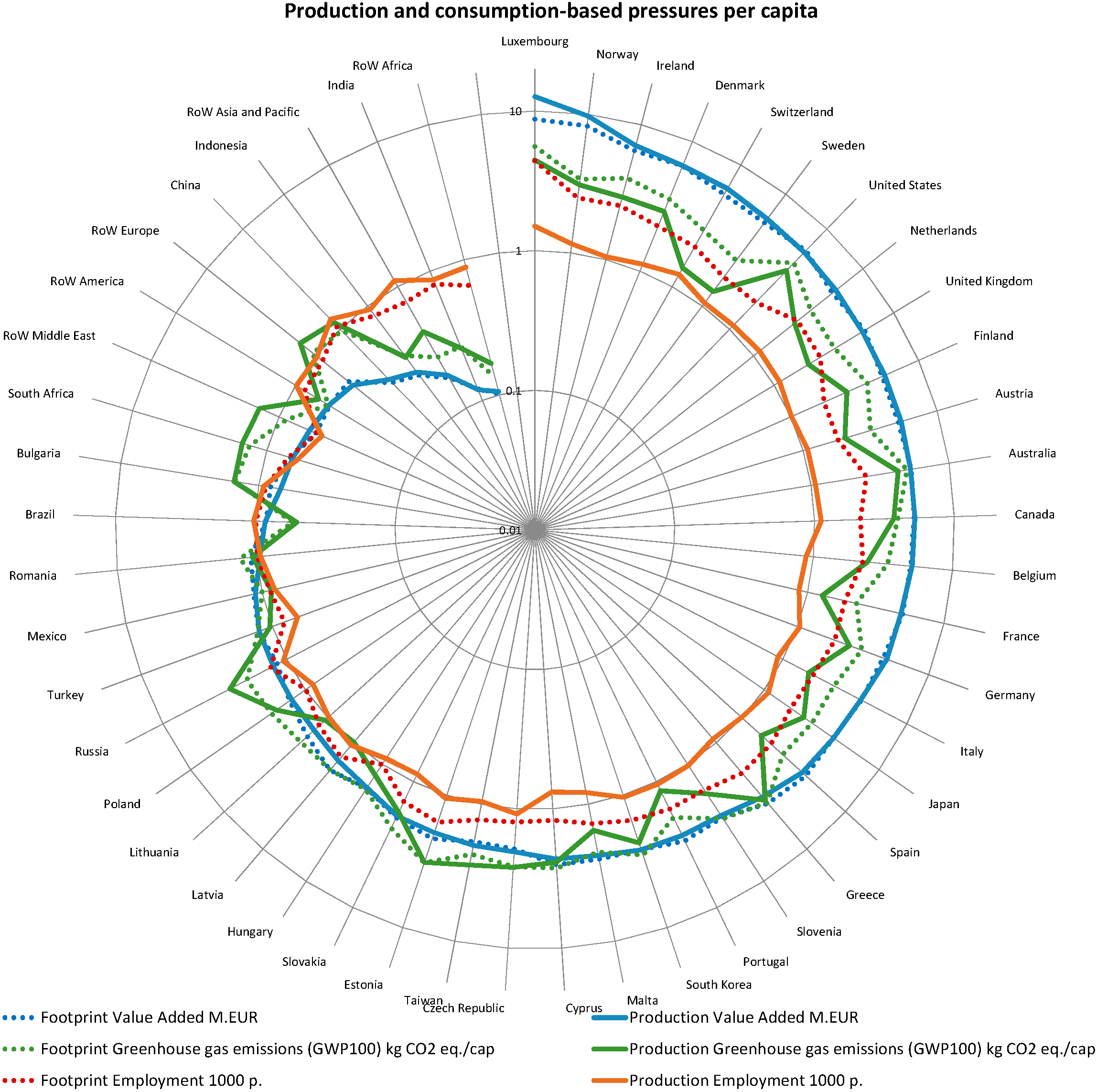
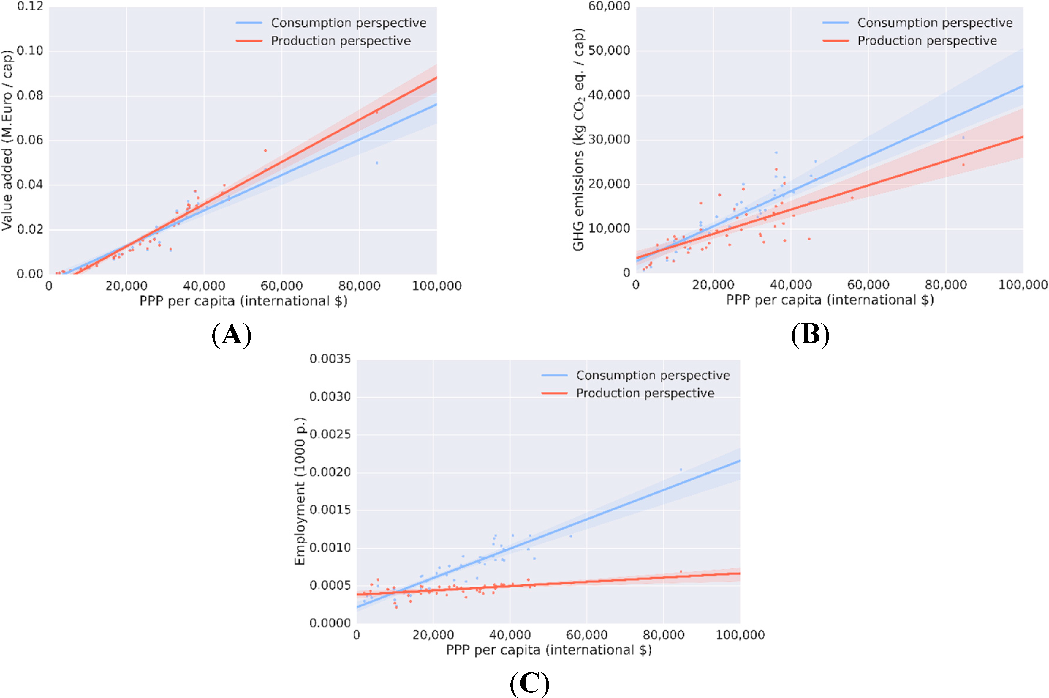
4.1. Sustainability Accounts—Production-Based versus Consumption-Based Indicators

Based on the integrated database, comparisons between production- and consumption-based accounts are readily available via Leontief modeling [26]. The production-based indicators account for the valued added as well as the substances emitted within the geographical bounds of a region or country. On the other hand, consumption-based indicators (footprints) represent the direct and indirect value added/emitted substances caused by the final demand in a specific country or region.

For value added, only marginal differences exist between the production versus the consumption perspective (Figure 2); relative to other indicators, there is very little value added embodied in trade. In contrast, employment accounts are significantly higher from a footprint perspective for wealthy countries. Only for the poorest countries and regions are there higher employee-years embodied in exports than imports. As for GHG emissions (100-year time horizon global warming potential applied [76]), demand-side emissions are generally higher than those of the supply side in industrialized countries, which indicates the existence of carbon leakage towards less industrialized countries.

Figure 2. Value added, employment and greenhouse gas emissions, production-based and consumption-based (footprint) account. The 100% line indicates the global average of the account per capita. Countries are ordered clockwise based on the GDP per capita; the percent values are plotted on logarithmic scale.

Figure 2. Value added, employment and greenhouse gas emissions, production-based and consumption-based (footprint) account. The 100% line indicates the global average of the account per capita. Countries are ordered clockwise based on the GDP per capita; the percent values are plotted on logarithmic scale.

To elaborate the relationship between wealth and the two perspectives, we investigate production and consumption accounts as a function of GDP per capita (purchasing power parity corrected).

For value added, wealthier countries tend to have more value added associated with the production on the territory than embodied in consumption (Figure 3A). However, it is the two wealthiest countries in the dataset (Norway and Luxembourg) that dictate this trend. The confidence intervals of both fits overlap significantly, thus indicating no clear separation of the two perspectives.

GHG emissions embodied in consumption, or the “carbon footprint” as it is commonly known, rise steadily with increasing income (Figure 3B). In addition, the divergence between the consumption and production perspective amplifies with higher wealth levels. Starting at about $20,000 per capita, almost all countries have higher GHG emissions embodied in consumption than those associated with the production within the country.

Figure 3. Production and consumption perspective in correlation to the wealth level (purchaser price parity, PPP, corrected GDP per capita). The shaded area corresponds to the 95% confidence band (based on 1000 bootstrap reiterations). (A) Value added; (B) GHG emissions; (C) Employment.

Figure 3. Production and consumption perspective in correlation to the wealth level (purchaser price parity, PPP, corrected GDP per capita). The shaded area corresponds to the 95% confidence band (based on 1000 bootstrap reiterations). (A) Value added; (B) GHG emissions; (C) Employment.

The highest deviation between the production and consumption perspective can be observed for employment (Figure 3C). Whereas the number of employees necessary for the production rises only marginally with higher income levels, wealthier countries rely on large amount of labor to satisfy their final demand.

Wealthier countries tend to be more efficient in the use of their labor force. They generate a high level of value added with almost the same amount of employment than poorer countries. This is probably due to the specialization on high revenue industries in developed countries (service sectors). However, consumers still demand products from primary and secondary sectors that depend on a higher degree of labor and GHG emissions during production. To a large extent, these products are imported from poorer countries, explaining the divergence between the production and consumption perspective for the employment and GHG accounts. Nevertheless, even for the GHG emissions associated with the production within a country, we could not find any sign of decoupling of environmental impact and wealth based on the EXIOBASE2 dataset. Furthermore, detailed results at the country level are available in the “Resource Footprint of Nations” [34].

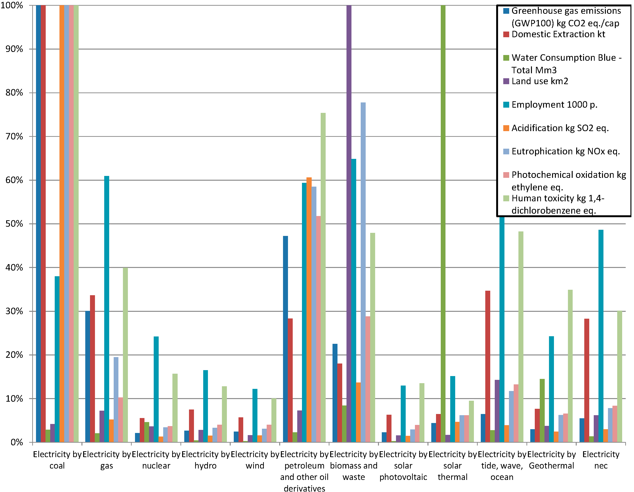
4.2. From Inventories to Impact Categories; Example of Electricity Supply

Macro-level (environmental) policy measures such as carbon taxation, implementation of energy standards, etc. will be enacted at the micro-level. Research investigating the effects of such macro-level policies is therefore supported by the ability of global databases to include specific technological choices [77]. A major focus of EXIOBASE2 was to link technological detail with economic and environmental intervention data for the whole world. This makes it possible to link the results from the IO calculations with a wide range of life cycle impact assessment indicators and compare between detailed industry sectors. A characterization matrix that allows for the easy calculation of the life cycle impact assessment indicators was used [38], which, because of the regional representation of environmental interventions, can include regionally specific characterization values. A helpful example is the impacts across the range of electricity technologies as illustrated in Figure 4 for the EU. In the figure, impacts across a range of impact categories are presented per unit output of electricity generation, normalized to the maximum value of each impact category. While coal clearly has the largest impact across most indicators (also seen in [77], biomass, considered by many a partial solution to the climate change issue, embodies other significant types of environmental impacts—identifying the potential for problem shifting. Similarly, the high technological costs of current state ocean-based technologies as of 2007 show relatively higher impacts (particularly employment at this stage of development). However, earlier life-cycle studies that focus on the longer term potential of the technology indicate greenhouse gas emissions could become lower than the average UK power mix generation [78] or electricity from wind turbines [79].

Figure 4. Impacts across the range of electricity generation technologies in EXIOBASE2, normalized to maximum impact of each indicator across the technologies.

Figure 4. Impacts across the range of electricity generation technologies in EXIOBASE2, normalized to maximum impact of each indicator across the technologies.

5. Conclusions

5.1. MRIO Development

Considerable progress is being made in MRIO development, and the existing options for global MRIO analyses have different, and often complementing, advantages and disadvantages [80]. EXIOBASE has its major strength in providing more sector detail compared to any other MRIO database, which in most cases only distinguish a small number of environmentally sensitive sectors. Furthermore, it includes by far the greatest amount of environmental data in a format consistent with the sector classification, whereas other MRIO datasets only include a small number of environmental issues, in most cases for calculating the carbon footprint [81]. An important disadvantage of the current EXIOBASE2 database is that it lacks a temporal dimension (2000 for EXIOBASEv1 and 2007 for EXIOBASE2), whereas other databases come with annual time series, for example for the period of 1995–2011 in the case of WIOD and 1990–2011 in EORA. However, with the currently ongoing revision of EXIOBASE towards version 3, an annual time series is also built for the period of 1995–2011, thus opening up a number of analytical options, including time series analysis and structural decompositions. Another limitation of EXIOBASE is the rather small number of countries/regions covered, which is comparable to the WIOD and OECD systems, but far below GTAP, which specifies 134 countries (version 8.1) or EORA with 187 countries. More detailed coverage of individual regions, especially in regard to environmentally distinct regions such as urban/rural divides and watersheds; higher levels of disaggregation of product groups and activities; greater possibilities to link into physical accounting databases, both at process level, and through datasets on physical consumption and production; and better representation of the temporal and stock dimension are all areas where we observe development to be headed. Further work on physical layers will allow physical allocation to take place, which will open up a broader set of analyses.

5.2. Sustainability Accounting

More generally, this paper focuses on the description of integrated accounting frameworks for the global mapping of environmental, economic and social impacts. Why is so much effort being put into these integrated frameworks? Clearly a development focus on increasing affluence is going to and has had serious environmental and social implications. By integrating different dimensions (such as resource extraction, employment and household demand) of the problems we face within a single accounting framework, the tools we have to confront relevant policy questions become more powerful. A full coverage of the different aspects of the sustainable development agenda is needed from a global perspective. We are not there yet, but are far more advanced than a decade ago; this paper describes one of the latest efforts to reach this goal.

The challenge for researchers will be to accurately model these large and complex systems and, equally important, to communicate results to governments and companies. MRIO frameworks are well suited for this and the increased coverage of environmental stressors in modern databases allows for detailed analyses of trade-offs between various environmental and socio-economic issues.

5.3. Globalization of Consumption

In pursuing sustainable development, we are increasingly seeing the need for a global approach in order to avoid problem shifting. Consumption in one country is inextricably linked to environmental impacts, wealth creation and labor use in other countries. The large inequalities that exist around the world are being exacerbated by trade as cheap labor and lenient emissions regulations in poorer countries are exploited by the wealthiest countries.

In trying to derive policy and drive consumer action on these issues, we need to raise consumer awareness of the indirect impacts of their consumption habits. Only by doing so can we ensure that informed choices are made and that the problems we strive to solve are not simply shifted from one place to another.

References

1. United Nations; European Union; Food and Agriculture Organization of the United Nations; International Monetary Fund; Organisation for Economic Co-operation and Development; The World Bank. System of Environmental-Economic Accounting 2012—Central Framework. Available online: http://unstats.un.org/unsd/envaccounting/White_cover.pdf (accessed on 15 December 2014).
2. Tukker, A.; Dietzenbacher, E. Global multiregional input-output frameworks: An introduction and outlook. Econ. Syst. Res. 2013, 25, 1–19. [Google Scholar] [CrossRef]
3. Isard, W. Interregional and regional input-output analysis, a model of a space economy. Rev. Econ. Stat. 1951, 33, 318–328. [Google Scholar] [CrossRef]
4. Polenske, K.R. Contributions to Input-Output Analysis: Fourth International Conference on Input-Output Techniques, 1970. In Empirical Implementation of a Multiregional Input-Output Gravity Trade Model; Carter, A.C., Bródy, A., Eds.; North-Holland Publishing Company: Amsterdam, The Netherlands, 1970; pp. 143–163. [Google Scholar]
5. Leontief, W.W.; Strout, A.A. Multiregional input-output analysis. In Structural Interdependence and Economic Development; Barna, T., Ed.; Macmillan: London, UK, 1963; pp. 119–149. [Google Scholar]
6. Munksgaard, J.; Pedersen, K.A. CO2 accounts for open economies: Producer or consumer responsibility? Energ. Pol. 2001, 29, 327–334. [Google Scholar] [CrossRef]
7. Lenzen, M.; Pade, L.L.; Munksgaard, J. CO2 multipliers in multi-region input-output models. Econ. Syst. Res. 2004, 16, 391–412. [Google Scholar] [CrossRef]
8. Turner, K.; Wiedmann, T.; Lenzen, M.; Barrett, J. Examining the global environmental impact of regional consumption activities—Part 1: A technical note on combining input-output and ecological footprint analysis. Ecol. Econ. 2007, 62, 37–44. [Google Scholar] [CrossRef]
9. Weinzettel, J.; Hertwich, E.G.; Peters, G.P.; Steen-Olsen, K.; Galli, A. Affluence drives the global displacement of land use. Global Environ. Chang. 2013, 23, 433–438. [Google Scholar] [CrossRef]
10. Hertwich, E.; Peters, G. Carbon footprint of nations: A global, trade-linked analysis. Environ. Sci. Technol. 2009, 43, 6414–6420. [Google Scholar] [CrossRef] [PubMed]
11. Peters, G.; Hertwich, E. CO2 embodied in international trade with implications for global climate policy. Environ. Sci. Technol. 2008, 42, 1401–1407. [Google Scholar] [CrossRef] [PubMed]
12. Kanemoto, K.; Moran, D.; Lenzen, M.; Geschke, A. International trade undermines national emission reduction targets: New evidence from air pollution. Glob. Environ. Chang. 2014, 24, 52–59. [Google Scholar] [CrossRef]
13. Skelton, A. EU corporate action as a driver for global emissions abatement: A structural analysis of EU international supply chain carbon dioxide emissions. Glob. Environ. Chang. 2013, 23, 1795–1806. [Google Scholar] [CrossRef]
14. Ewing, B.R.; Hawkins, T.R.; Wiedmann, T.O.; Galli, A.; Ertug Ercin, A.; Weinzettel, J.; Steen-Olsen, K. Integrating ecological and water footprint accounting in a multi-regional input-output framework. Ecol. Indicators 2012, 23, 1–8. [Google Scholar] [CrossRef] [Green Version]
15. Tukker, A.; Koning, A.D.; Wood, R.; Hawkins, T.; Lutter, S.; Acosta, J.; Rueda Cantuche, J.M.; Bouwmeester, M.; Oosterhaven, J.; Dosdrowski, T.; et al. Exiopol—Development and illustrative analyses of a detailed global MR EE SUT/IOT. Econ. Syst. Res. 2013, 25, 50–70. [Google Scholar] [CrossRef]
16. OECD; WTO; UNCTAD. Implications of global value chains for trade, investment, development and jobs. Available online: http://www.oecd.org/sti/ind/G20-Global-Value-Chains-2013.pdf (accessed on 15 December 2014).
17. Lenzen, M.; Moran, D.; Kanemoto, K.; Foran, B.; Lobefaro, L.; Geschke, A. International trade drives biodiversity threats in developing nations. Nature 2012, 486, 109–112. [Google Scholar] [CrossRef] [PubMed]
18. Simas, M.; Wood, R.; Hertwich, E. Labor embodied in trade: The role of labor and energy productivity and implications for greenhouse gas emissions. J. Ind. Ecol. 2014, in press. [Google Scholar]
19. Simas, M.; Golsteijn, L.; Huijbregts, M.; Wood, R.; Hertwich, E. The “bad labor” footprint: Quantifying the social impacts of globalisation. Sustainability 2014, 6, 7514–7540. [Google Scholar] [CrossRef] [Green Version]
20. Huysman, S.; Schaubroeck, T.; Dewulf, J. Quantification of spatially differentiated resource footprints for products and services through a macro-economic and thermodynamic approach. Environ. Sci. Technol. 2014, 48, 9709–9716. [Google Scholar] [CrossRef] [PubMed]
21. Dietzenbacher, E.; Los, B.; Stehrer, R.; Timmer, M.; de Vries, G. The construction of world input-output tables in the wiod project. Econ. Syst. Res. 2013, 25, 71–98. [Google Scholar] [CrossRef]
22. Lenzen, M.; Moran, D.; Kanemoto, K.; Geschke, A. Building eora: A global multi-region input-output database at high country and sector resolution. Econ. Syst. Res. 2013, 25, 20–49. [Google Scholar] [CrossRef]
23. Narayanan, G.; Badri, A.A.; McDougall, R. Global Trade, Assistance, and Production: The Gtap 8 Data Base. Available online: https://www.gtap.agecon.purdue.edu/databases/v8/v8_doco.asp (accessed on 15 December 2014).
24. Nakano, S.; Okamura, A.; Sakurai, N.; Suzuki, M.; Tojo, Y.; Yamano, N. The Measurement of CO2 Embodiments in International Trade: Evidence from the Harmonised Input-Output and Bilaterial Trade Database; Organisation for Economic Co-operation and Development (OECD): Paris, France, 2009. [Google Scholar]
25. Pulles, T.; van het Bolscher, M.; Brand, R.; Visschedijk, A. Assessment of Global Emissions from Fuel Combustion in the Final Decades of the 20th Century; TNO Built Environment and Geosciences: Apeldoorn, The Netherlands, 2007. [Google Scholar]
26. Murray, J.; Wood, R. The Sustainability Practitioner’s Guide to Input-Output Analysis; Common Ground Publications: Champaign, IL, USA, 2010. [Google Scholar]
27. Steen-Olsen, K.; Owen, A.; Hertwich, E.G.; Lenzen, M. Effects of sector aggregation on CO2 multipliers in multiregional input-output analyses. Econ. Syst. Res. 2014, 26, 284–302. [Google Scholar] [CrossRef]
28. EXIOBASE. Available online: www.exiobase.eu (accessed on 23 December 2014).
29. Tukker, A.; Poliakov, E.; Heijungs, R.; Hawkins, T.; Neuwahl, F.; Rueda-Cantuche, J.M.; Giljum, S.; Moll, S.; Oosterhaven, J.; Bouwmeester, M. Towards a global multi-regional environmentally extended input-output database. Ecol. Econ. 2009, 68, 1928–1937. [Google Scholar] [CrossRef]
30. Wood, R.; Hawkins, T.R.; Hertwich, E.G.; Tukker, A. Harmonising national input-output tables for consumption-based accounting—Experiences from exiopol. Econ. Syst. Res. 2014, 26, 387–409. [Google Scholar] [CrossRef]
31. Tukker, A.; Bulavskaya, T.; Giljum, S.; de Koning, A.; Lutter, S.; Simas, M.; Stadler, K.; Wood, R. The Global Resource Footprint of Nations—Carbon, Water, Land and Materials Embodied in Trade and Final Consumption Calculated with Exiobase 2.1. Available online: http://www.exiobase.eu/9-home/27-creea-booklet (accessed on 15 December 2014).
32. CREEA. Available online: http://www.creea.eu/ (accessed on 23 December 2014).
33. DESIRE. Available online: www.fp7desire.eu (accessed on 23 December 2014).
34. Merciai, S.; Schmidt, J.H.; Dalgaard, R.; Giljum, S.; Lutter, S.; Usubiaga, A.; Acosta, J.; Schutz, H.; Wittmer, D.; Delahaye, R. Report and Data Task 4.2: P-Sut. Available online: http://www.creea.eu/index.php/documents2/doc_download/47-deliverable-42 (accessed on 15 December 2014).
35. Fischer-Kowalski, M. Society’s metabolism: The intellectual history of materials flow analysis, part I, 1860–1970. J. Ind. Ecol. 1998, 2, 61–78. [Google Scholar] [CrossRef]
36. Pauliuk, S.; Wood, R.; Hertwich, E.G. Dynamic models of fixed capital stocks and their application in industrial ecology. J. Ind. Ecol. 2014. Available online: http://onlinelibrary.wiley.com/doi/10.1111/jiec.12149/abstract (accessed on 12 December 2014). [CrossRef] [Green Version]
37. Heijungs, R.; Suh, S. The Computational Structure of Life Cycle Assessment; Kluwer Academic Publishers: Dordrecht, The Netherlands, 2002. [Google Scholar]
38. Schoer, K.; Wood, R.; Arto, I.; Weinzettel, J. Estimating raw material equivalents on a macro-level: Comparison of multi-regional input-output analysis and hybrid lci-io. Environ. Sci. Technol. 2013, 47, 14282–14289. [Google Scholar] [CrossRef] [PubMed]
39. Bruckner, M.; Giljum, S.; Lutz, C.; Wiebe, K.S. Materials embodied in international trade—Global material extraction and consumption between 1995 and 2005. Glob. Environ. Chang. 2012, 22, 568–576. [Google Scholar] [CrossRef]
40. Wood, R.; Lenzen, M.; Foran, B. A material history of australia: Evolution of material intensity and drivers of change. J. Ind. Ecol. 2009, 13, 847–862. [Google Scholar] [CrossRef]
41. United Nations Statistics Division. System of National Accounts 1993; United Nations Statistics Division (UNSD): New York, NY, USA, 1993. [Google Scholar]
42. United Nations Statistics Division. Un Comtrade—United Nations Commodity Trade Statistics Database; United Nations Statistics Division (UNSD): New York, NY, USA, 2012. [Google Scholar]
43. United Nations Statistics Division. United Nations Service Trade Statistics Database; United Nations Statistics Division (UNSD): New York, NY, USA, 2012. [Google Scholar]
44. Gaulier, G.; Zignago, S. BACI: International Trade Database at the Product-Level. Available online: http://www.cepii.fr/CEPII/en/publications/wp/abstract.asp?NoDoc=2726 (accessed on 15 December 2014).
45. Müller, M.; Pérez Domínguez, I.; Gay, S.H. Construction of social accounting matrices for EU27 with a disaggregated agricultural sector (agrosams). Available online: http://ipts.jrc.ec.europa.eu/publications/pub.cfm?id=2679 (accessed on 12 December 2014).
46. FAO Statistics Division (FAOSTAT). Prodstat; Food and Agriculture Organization of the United Nations: Rome, Italy, 2012. [Google Scholar]
47. Eurostat. Prodcom. Eurostat—Statistical Office of the European Union (ESTAT). Available online: http://epp.eurostat.ec.europa.eu/portal/page/portal/prodcom/data/database (accessed on 22 December 2014).
48. Eurostat. Structural Business Statistics. Eurostat—Statistical Office of the European Union (ESTAT). Available online: http://ec.europa.eu/eurostat/web/structural-business-statistics/structural-business-statistics (accessed on 22 December 2014).
49. International Energy Agency (IEA). Energy Balances: Non-OECD; OECD/IEA: Paris, France, 2012. [Google Scholar]
50. International Energy Agency (IEA). Energy Balances: OECD; OECD/IEA: Paris, France, 2012. [Google Scholar]
51. United Nations Department of Economic and Social Affairs (UNDESA). System of Environmental-Economic Accounting for Energy. Seea-Energy. Available online: http://unstats.un.org/unsd/envaccounting/seeaE/GC_Draft.pdf (accessed on 20 December 2014).
52. Eurostat. Physical energy flow accounts (pefa)—Manual 2014. Available online: http://epp.eurostat.ec.europa.eu/portal/page/portal/environmental_accounts/documents/PEFA_Manual_2014_v20140515.pdf (accessed on 12 December 2014).
53. Kuenen, J.; Fernández, J.A.; Usubiaga, A.; Wittmer, D. Report on Update Exiopol Emissions Database. Available online: http://www.creea.eu/index.php/documents2/doc_download/39-deliverable-61 (accessed on 15 December 2014).
54. Eurostat. Manual for air emissions accounts. Available online: http://epp.eurostat.ec.europa.eu/cache/ITY_OFFPUB/KS-RA-09-004/EN/KS-RA-09-004-EN.PDF (accessed on 12 December 2014).
55. Intergovernmental Panel on Climate Change (IPCC). IPCC guidelines for national greenhouse gas inventories. Available online: http://www.ipcc-nggip.iges.or.jp/public/2006gl/ (accessed on 15 December 2014).
56. European Environment Agency (EEA). Emep/eea Air Pollutant Emission Inventory Guidebook 2009; Publications Office of the European Union: Luxembourg, 2009. [Google Scholar]
57. International Labour Organization (ILO). Laborsta—Database on labour statistics. Available online: http://laborsta.Ilo.org (accessed on 12 December 2014).
58. Organisation for Economic Co-operation and Development (OECD). Stan database for structural analysis. Available online: http://stats.Oecd.Org/index.Aspx?Datasetcode=stan08bis (accessed on 12 December 2014).
59. Lutter, S.; Mekkonnen, M.; Raptis, C. Updated and improved data on water consumption/use imported into the exiobase in the required sectoral (dis)aggregation. Available online: http://209.116.186.231/url?sa=t&rct=j&q=Updated%20and%20improved%20data%20on%20water%20consumption%2Fuse%20imported%20into%20the%20exiobase%20in%20the%20required%20sectoral%20(dis)aggregation&source=web&cd=1&ved=0CBsQFjAA&url=http%3a%2f%2fcreea%2eeu%2findex%2ephp%2fdocuments2%2fdoc_download%2f33-deliverable-34&ei=mniKVM_aFZSzyASk8YGwDQ&usg=AFQjCNG1gpHB7P59tpNL51WRbpI3tfnCHA&cad=rja (accessed on 12 December 2014).
60. Flörke, M.; Kynast, E.; Bärlund, I.; Eisner, S.; Wimmera, F.; Alcamo, J. Domestic and industrial water uses of the past 60 years as a mirror of socio-economic development: A global simulation study. Glob. Environ. Change 2013, 23, 144–156. [Google Scholar] [CrossRef]
61. Sustainable Europe Research Institute (SERI). Global material flow database. Available online: http://www.Materialflows.net (accessed on 15 December 2014).
62. Eurostat. Economy-wide material flow accounts (ew-mfa). Available online: http://epp.eurostat.ec.europa.eu/portal/page/portal/environmental_accounts/publications/economy_wide_material_flow_accounts (accessed on 12 December 2014).
63. OECD. Measuring Material Flows and Resource Productivity; Organisation for Economic Cooperation and Development: Paris, France, 2008. [Google Scholar]
64. Wood, R.; Bulavskaya, T.; Ivanova, O.; Stadler, K.; Simas, M.; Tukker, A.; Lutter, S.; Kuenen, J.; Heijungs, R. Report d7.2 update exiobase with wp3–6 input. Available online: http://www.creea.eu/index.php/documents2/doc_download/44-deliverable-72 (accessed on 15 December 2014).
65. Stadler, K.; Wood, R.; Steen-Olsen, K. The “rest of the world”—Estimating the economic structure of missing regions in global mrio tables. Econ. Syst. Res. 2014, 26, 303–326. [Google Scholar] [CrossRef]
66. Institute of Communication and Computer Systems (ICCS). MODELS—MOdel Development for the Evaluation of LisbonStrategies. Available online: http://www.ecmodels.eu/index_files/MODELS_Final%20Publishable%20Report.pdf (accessed on 20 December 2014).
67. Burns, S. Cost build up model for primary aluminum ingot production. Available online: http://agmetalminer.com/2009/02/27/cost-build-up-model-for-primary-aluminum-ingot-production/ (accessed on 12 December 2014).
68. Jackson, R.W.; Murray, A.T. Alternative input-output matrix updating formulations. Econ. Syst. Res. 2004, 16, 135–148. [Google Scholar] [CrossRef]
69. Lenzen, M.; Gallego, B.; Wood, R. A flexible approach to matrix balancing under partial information. J. Appl. Input-Output Anal. 2006, 11–12, 1–24. [Google Scholar]
70. Bacharach, M. Biproportional Matrices & Input-Output Change; Cambridge University Press: Cambridge, UK, 1970; Volume 16. [Google Scholar]
71. Lecomber, J.R.C. A critique of methods of adjusting, updating and projecting matrices, together with some new proposals. In Input-Output and Throughput: Proceedings of the 1971 Norwich Conference; Gossling, W.F., Ed.; Input-Output Publishing Company: London, UK, 1975; pp. 90–100. [Google Scholar]
72. United Nations Statistics Division. National Accounts Main Aggregates Database; United Nations Statistics Division (UNSD): New York, NY, USA, 2013. [Google Scholar]
73. Bouwmeester, M.C. Economics and environment—Modelling global linkages. Ph.D. Thesis, Groningen University, Groningen, The Netherlands, 2014. [Google Scholar]
74. Junius, T.; Oosterhaven, J. The solution of updating or regionalizing a matrix with both positive and negative entries. Econ. Syst. Res. 2003, 15, 87–96. [Google Scholar] [CrossRef]
75. Lenzen, M.; Wood, R.; Gallego, B. Some comments on the gras method. Econ. Syst. Res. 2007, 19, 461–465. [Google Scholar] [CrossRef]
76. Intergovernmental Panel on Climate Change (IPCC). IPCC Fourth Assessment Report: Climate Change 2007—Working Group I: The Physical Science Basis; Intergovernmental Panel on Climate Change: Geneva, Switzerland, 2007. [Google Scholar]
77. Hertwich, E.G.; Gibon, T.; Bouman, E.A.; Arvesen, A.; Suh, S.; Heath, G.A.; Bergesen, J.D.; Ramirez, A.; Vega, M.I.; Shi, L. Integrated life-cycle assessment of electricity-supply scenarios confirms global environmental benefit of low-carbon technologies. Proc. Natl. Acad. Sci. 2014, in press. [Google Scholar]
78. Kelly, K.A.; McManus, M.C.; Hammond, G.P. An energy and carbon life cycle assessment of tidal power case study: The proposed cardiff-weston severn barrage scheme. Energy 2012, 44, 692–701. [Google Scholar] [CrossRef] [Green Version]
79. Rule, B.M.; Worth, Z.J.; Boyle, C.A. Comparison of life cycle carbon dioxide emissions and embodied energy in four renewable electricity generation technologies in New Zealand. Environ. Sci. Technol. 2009, 43, 6406–6413. [Google Scholar] [CrossRef] [PubMed]
80. Inomata, S.; Owen, A. Comparative evaluation of mrio databases. Econ. Syst. Res. 2014, 26, 239–244. [Google Scholar] [CrossRef]
81. Moran, D.; Wood, R. Convergence between the Eora, WIOD, EXIOBASE, and OpenEU’s consumption-based carbon accounts. Econ. Syst. Res. 2014, 26, 245–261. [Google Scholar] [CrossRef]