Carbon Emissions Abatement Cost in China: Provincial Panel Data Analysis

Abstract
:1. Introduction
2. Methodology
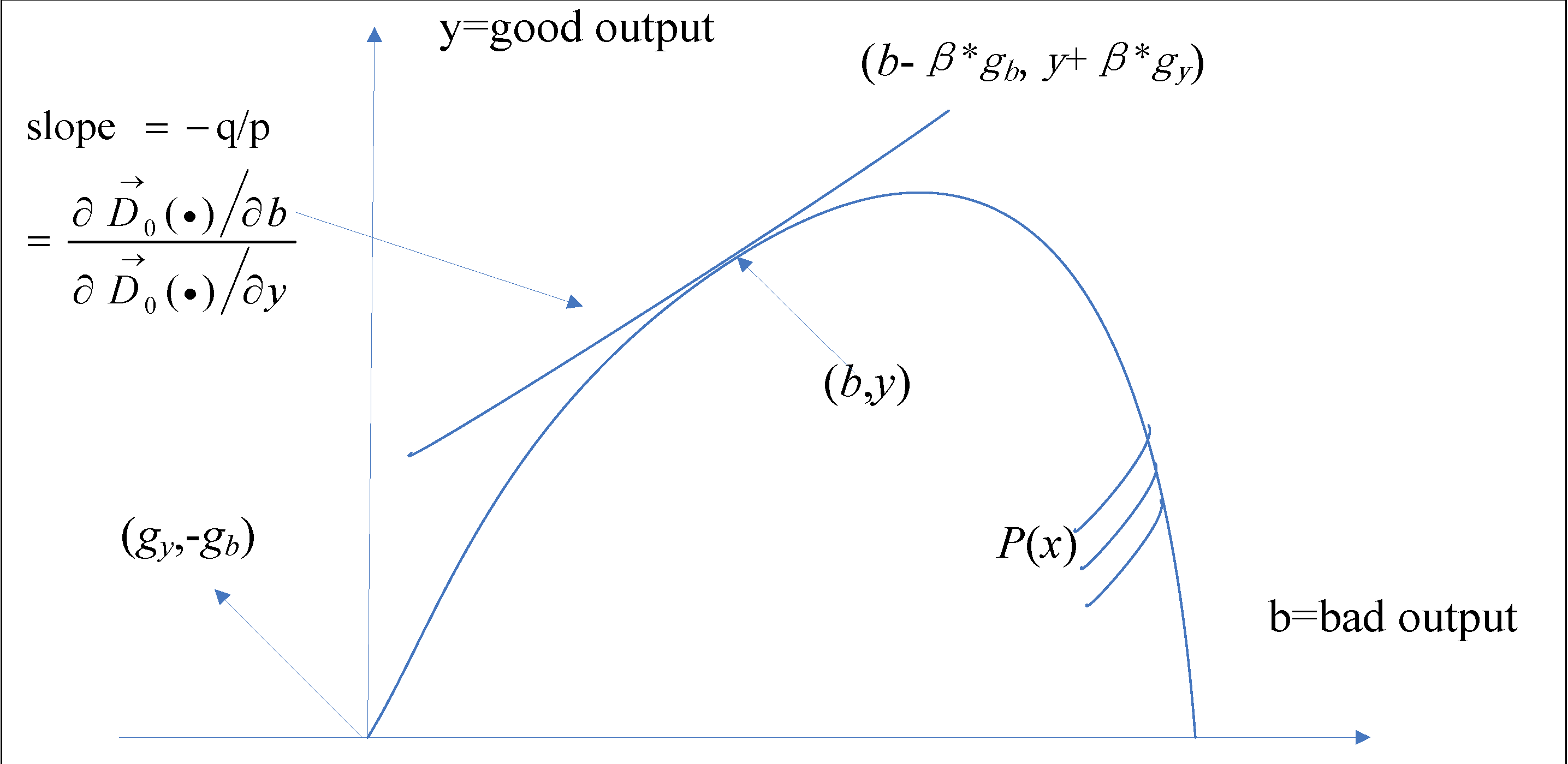
2.1. The Directional Output Distance Function
 (x, y, b; gy, gb) = max {β : (y + βgy,b − βgb ∊ P(x)}
(x, y, b; g). The shadow price ratio for the observation unit with coordinates (b, y) is provided by the slope of the tangent line estimated on the frontier of P(x).
(x, y, b; gy, gb) = max {β : (y + βgy,b − βgb ∊ P(x)}
(x, y, b; g). The shadow price ratio for the observation unit with coordinates (b, y) is provided by the slope of the tangent line estimated on the frontier of P(x). (x, y + αgy, b − αgb; g) = (x, y, b; g) − α ,
 ,
,
2.2. The Shadow Price Model
(x, y, b; gy, gb) ≥ 0. Based on this point, the revenue function can also be described as
 ,
(x, y, b; g)·gy, b − (x, y, b; g)·gb) ∊ P(x)}
(x, y, b; g)·gy,b − (x, y, b; g)·gb) − lx,
(x, y, b; g)·gy + q (x, y, b; g)·gb ,
(x, y, b; g)·gy. The other is generated due to bad output reductions, i.e., q (x, y, b; g)·gb. If the decision-making unit moves along a direction vector to the frontier of P(x), the output allocation is efficient and then the inequality (12) will become the equality.
,
(x, y, b; g)·gy, b − (x, y, b; g)·gb) ∊ P(x)}
(x, y, b; g)·gy,b − (x, y, b; g)·gb) − lx,
(x, y, b; g)·gy + q (x, y, b; g)·gb ,
(x, y, b; g)·gy. The other is generated due to bad output reductions, i.e., q (x, y, b; g)·gb. If the decision-making unit moves along a direction vector to the frontier of P(x), the output allocation is efficient and then the inequality (12) will become the equality. ,
,
 ,
,
 ,
,
 ,
,
 ,
,
3. Empirical Analysis
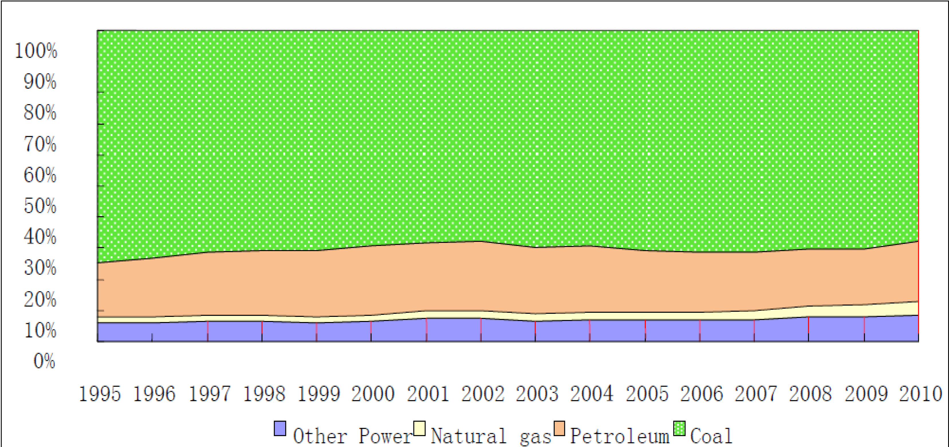
3.1. Data and Variables
 ,
,

| Variable | Units | Mean | St. Dev. | Min. | Max. |
|---|---|---|---|---|---|
| Output | |||||
| y = GDP | 108 Yuan | 5301.20 | 5139.41 | 195.68 | 30,219.33 |
| B = CO2 emission | 104 ton | 22,666.88 | 18,292.02 | 659.03 | 111,400.50 |
| Input | |||||
| x1 = Labor force | 104 person | 1768.30 | 1157.93 | 171.94 | 6173.20 |
| x2 = Capital | 108 Yuan | 5372.94 | 4463.78 | 240.06 | 23,038.26 |
| x3 = Energy consumption | 104 TCE | 7816.45 | 5916.36 | 390.30 | 34,807.77 |
3.2. The Shadow Price Estimation
3.2.1. The Quadratic Distance Function Form

 ,
,
 ,
,
- (i)
![Sustainability 06 02584 i025]() ≥ 0, k = 1,...,K, t = 1,...,T
≥ 0, k = 1,...,K, t = 1,...,T- (ii)
- ∂
![Sustainability 06 02584 i025]() /∂y ≤ 0, k = 1,...,K,t = 1,...,T
/∂y ≤ 0, k = 1,...,K,t = 1,...,T - (iii)
- ∂
![Sustainability 06 02584 i025]() /∂b ≥ 0, k = 1,...,K,t = 1,...,T
/∂b ≥ 0, k = 1,...,K,t = 1,...,T - (iv)
- c1 − c2 = −1, α = β = μ, δn − ηn = 0, n = 1,2,3
- (v)
- cn,n’ = cn’ ,n, n = 1,2,3

 (x, y, b;1,−1) ≥ 0. Thus, the null-jointness can be tested by observing the values of (x, y, 0;1,−1) for y > 0. If (x, y, 0;1,−1) < 0, (y,0) ∉ P(x), then the property of null-jointness is feasible. Without undesirable outputs, there are no desirable outputs, and the two ones are jointly produced. The test results indicate that the null-jointness condition is satisfied for 89.3% of the observations (375/420), which is an acceptable result to guarantee the following calculation.
| Parameter | Variable | Value | Parameter | Variable | Value |
|---|---|---|---|---|---|
| c0 | 1 | −0.0295 | c31 | 1/2x3x1 | 0.5655 |
| d1 | x1 | 0.7057 | c32 | 1/2x3x2 | 0.0025 |
| d2 | x2 | 0.4018 | c33 | 1/2x3x3 | −0.1057 |
| d3 | x3 | −0.2890 | α | 1/2yy | −0.0219 |
| c1 | y | −0.7287 | β | 1/2bb | −0.0219 |
| c2 | b | 0.2713 | δ1 | x1y | −0.1547 |
| c11 | 1/2x1x1 | −0.7193 | δ2 | x2y | 0.2946 |
| c12 | 1/2x1x2 | 0.2394 | δ3 | x3y | −0.1535 |
| c13 | 1/2x1x3 | 0.5655 | η1 | x1b | −0.1547 |
| c21 | 1/2x2x1 | 0.2394 | η2 | x2b | 0.2946 |
| c22 | 1/2x2x2 | −0.7523 | η3 | x3b | −0.1535 |
| c23 | 1/2x2x3 | 0.0025 | μ | yb | −0.0219 |
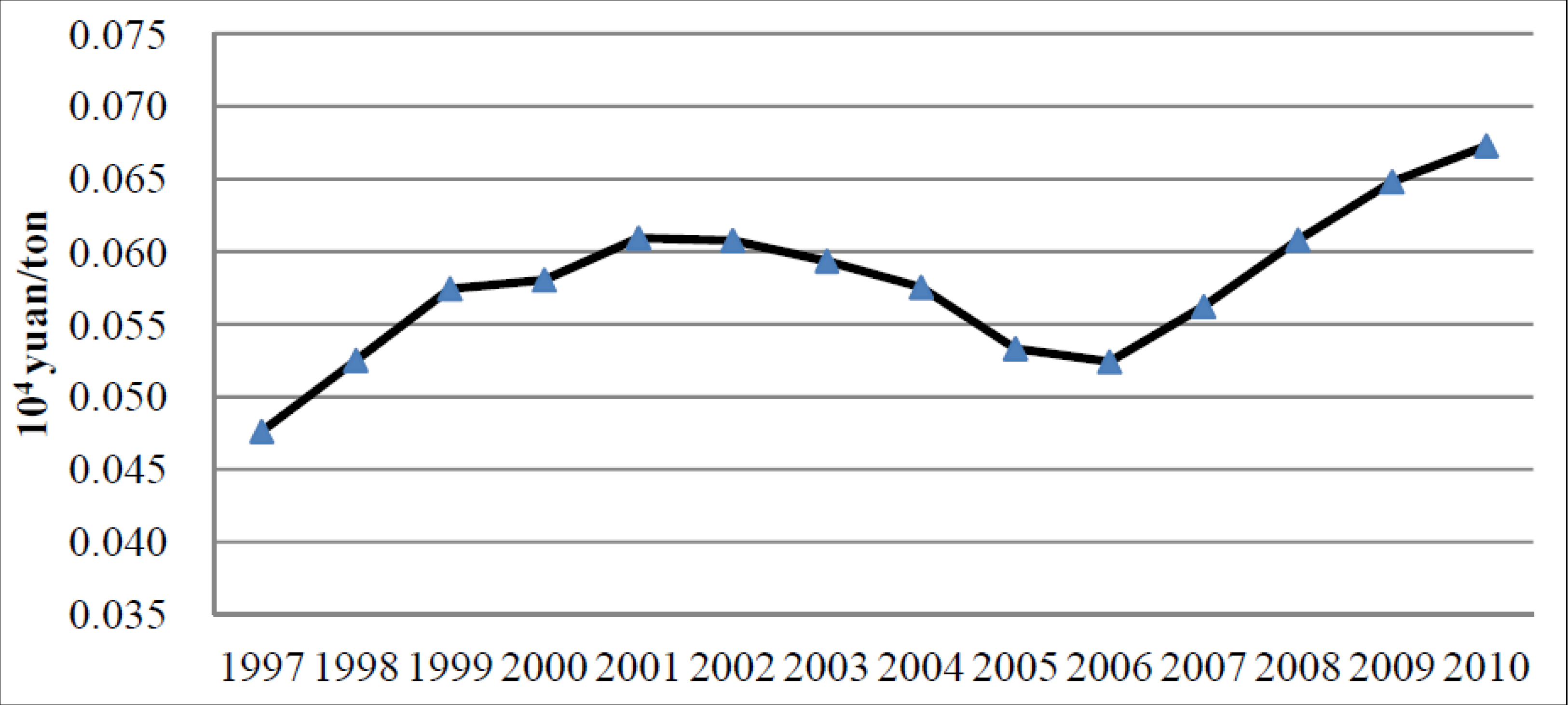
3.2.2. The Analysis of Results
| Areas | Provinces | 1997 | 1998 | 1999 | 2000 | 2001 | 2002 | 2003 | 2004 | 2005 | 2006 | 2007 | 2008 | 2009 | 2010 | average |
|---|---|---|---|---|---|---|---|---|---|---|---|---|---|---|---|---|
| SE | Shanghai | 1697 | 1959 | 2137 | 2206 | 2342 | 2525 | 2537 | 2641 | 2642 | 2750 | 2946 | 3169 | 3447 | 3612 | 2706 |
| Jiangsu | 1562 | 1565 | 1541 | 1375 | 1405 | 1454 | 1374 | 1255 | 1034 | 1037 | 1102 | 1204 | 1267 | 1233 | 1258 | |
| Zhejiang | 877 | 1005 | 1014 | 982 | 1086 | 1006 | 999 | 1025 | 1012 | 1032 | 1095 | 1217 | 1340 | 1306 | 1112 | |
| Hainan | 800 | 873 | 943 | 976 | 1017 | 1022 | 998 | 982 | 951 | 958 | 1008 | 1081 | 1141 | 1182 | 1050 | |
| Fujian | 698 | 791 | 859 | 863 | 964 | 908 | 894 | 897 | 871 | 879 | 932 | 978 | 1006 | 1034 | 928 | |
| Guangdong | 676 | 737 | 803 | 786 | 780 | 846 | 835 | 794 | 673 | 626 | 658 | 732 | 804 | 880 | 759 | |
| NC | Beijing | 1254 | 1398 | 1550 | 1641 | 1719 | 1857 | 1911 | 1912 | 1863 | 1900 | 2028 | 2187 | 2305 | 2308 | 1881 |
| Hebei | 282 | 294 | 304 | 234 | 329 | 171 | 145 | 139 | 105 | 116 | 122 | 149 | 164 | 175 | 175 | |
| Tianjin | 754 | 814 | 864 | 890 | 918 | 964 | 970 | 954 | 936 | 942 | 993 | 1037 | 1065 | 1050 | 959 | |
| Shandong | 236 | 285 | 338 | 255 | 420 | 189 | 196 | 183 | 98 | 97 | 124 | 153 | 169 | 222 | 183 | |
| MY | Anhui | 405 | 444 | 427 | 453 | 455 | 507 | 549 | 568 | 585 | 595 | 627 | 649 | 670 | 734 | 577 |
| Jiangxi | 488 | 541 | 577 | 594 | 614 | 579 | 546 | 538 | 521 | 525 | 561 | 594 | 610 | 637 | 571 | |
| Hubei | 302 | 352 | 395 | 383 | 459 | 499 | 504 | 504 | 528 | 555 | 603 | 660 | 699 | 683 | 541 | |
| Hunan | 232 | 257 | 389 | 412 | 385 | 382 | 359 | 320 | 254 | 296 | 308 | 328 | 341 | 304 | 319 | |
| NW | Gansu | 424 | 438 | 449 | 483 | 520 | 531 | 521 | 518 | 504 | 513 | 551 | 596 | 644 | 651 | 540 |
| Ningxia | 568 | 621 | 676 | 720 | 751 | 752 | 688 | 674 | 658 | 664 | 707 | 757 | 800 | 824 | 726 | |
| Qinghai | 605 | 658 | 690 | 735 | 765 | 779 | 768 | 747 | 713 | 719 | 763 | 813 | 865 | 895 | 773 | |
| Xinjiang | 567 | 634 | 710 | 767 | 807 | 861 | 861 | 841 | 815 | 827 | 880 | 938 | 990 | 1029 | 862 | |
| MYR | Shanxi | 72 | 85 | 113 | 133 | 38 | 11 | 30 | 35 | 36 | 36 | 37 | 82 | 136 | 155 | 69 |
| Henan | 411 | 367 | 370 | 380 | 358 | 371 | 332 | 246 | 234 | 211 | 201 | 199 | 208 | 218 | 261 | |
| Shaanxi | 512 | 553 | 642 | 690 | 660 | 664 | 654 | 639 | 612 | 613 | 646 | 671 | 696 | 711 | 652 | |
| Inner Mongolia | 352 | 412 | 373 | 444 | 416 | 433 | 375 | 305 | 243 | 189 | 204 | 180 | 166 | 168 | 245 | |
| NE | Liaoning | 95 | 126 | 131 | 102 | 139 | 275 | 338 | 343 | 409 | 428 | 464 | 490 | 520 | 552 | 357 |
| Jilin | 221 | 303 | 354 | 414 | 445 | 457 | 462 | 494 | 553 | 567 | 610 | 643 | 689 | 731 | 532 | |
| Heilongjiang | 127 | 168 | 191 | 249 | 297 | 376 | 413 | 446 | 475 | 504 | 560 | 597 | 652 | 710 | 450 | |
| SW | Chongqing | 361 | 335 | 332 | 504 | 468 | 537 | 529 | 519 | 451 | 460 | 484 | 505 | 519 | 529 | 476 |
| Guangxi | 427 | 485 | 542 | 583 | 634 | 651 | 643 | 592 | 582 | 583 | 600 | 616 | 632 | 676 | 603 | |
| Guizhou | 268 | 249 | 291 | 296 | 304 | 356 | 309 | 319 | 387 | 395 | 418 | 452 | 472 | 499 | 379 | |
| Sichuan | 265 | 292 | 382 | 469 | 469 | 490 | 414 | 385 | 433 | 445 | 478 | 505 | 511 | 520 | 448 | |
| Yunnan | 473 | 530 | 595 | 637 | 675 | 660 | 669 | 641 | 614 | 626 | 675 | 720 | 754 | 794 | 671 | |
| National average | 331 | 344 | 400 | 463 | 475 | 509 | 471 | 457 | 481 | 489 | 519 | 549 | 566 | 594 | 475 | |


 ,
,
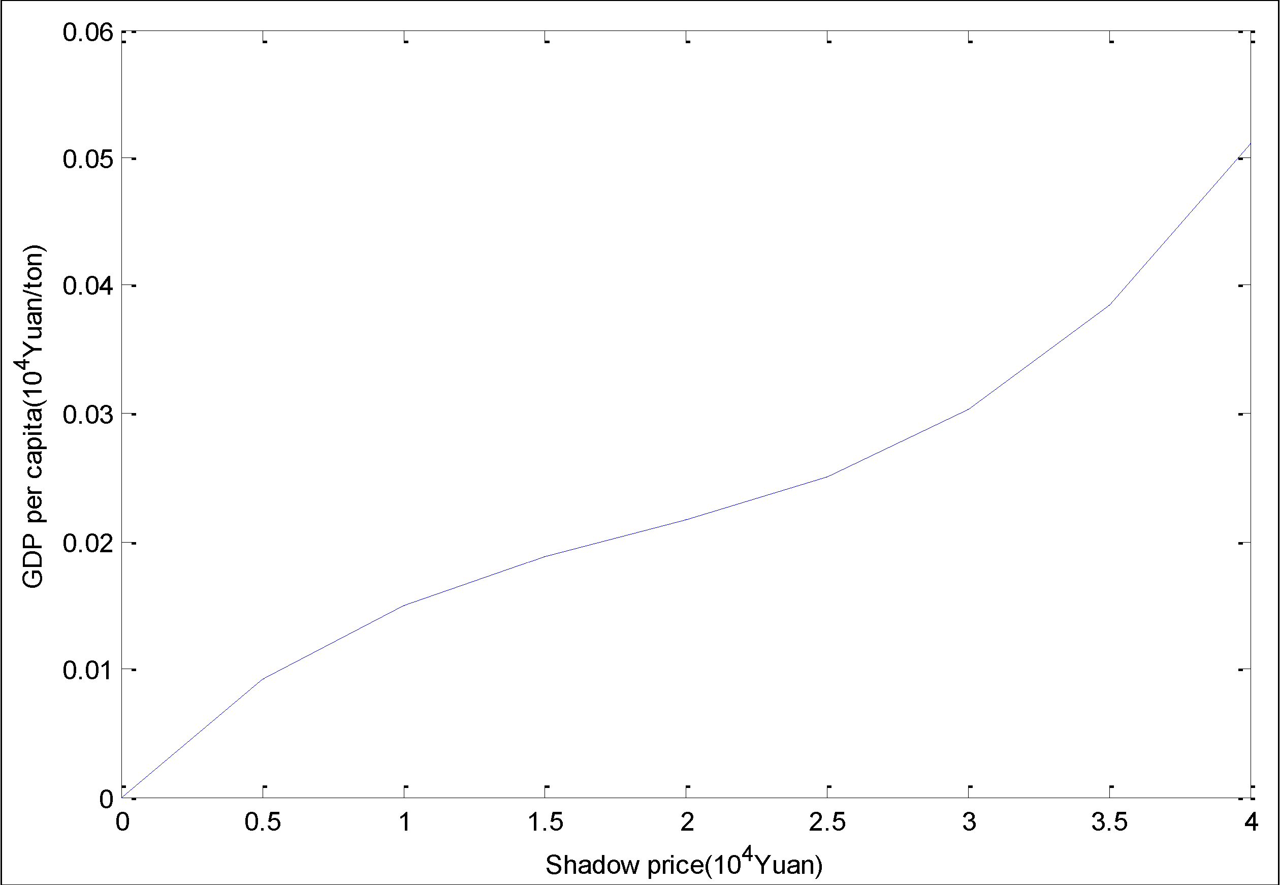
| Variable | Coefficient | Std. Error | T-Statistic | p-value |
|---|---|---|---|---|
| GDPPC | 0.022561 | 0.005073 | 4.446912 | 0.0000 |
| GDPPC2 | −0.009277 | 0.002309 | −4.016974 | 0.0001 |
| GDPPC3 | 0.001708 | 0.000292 | 5.848056 | 0.0000 |

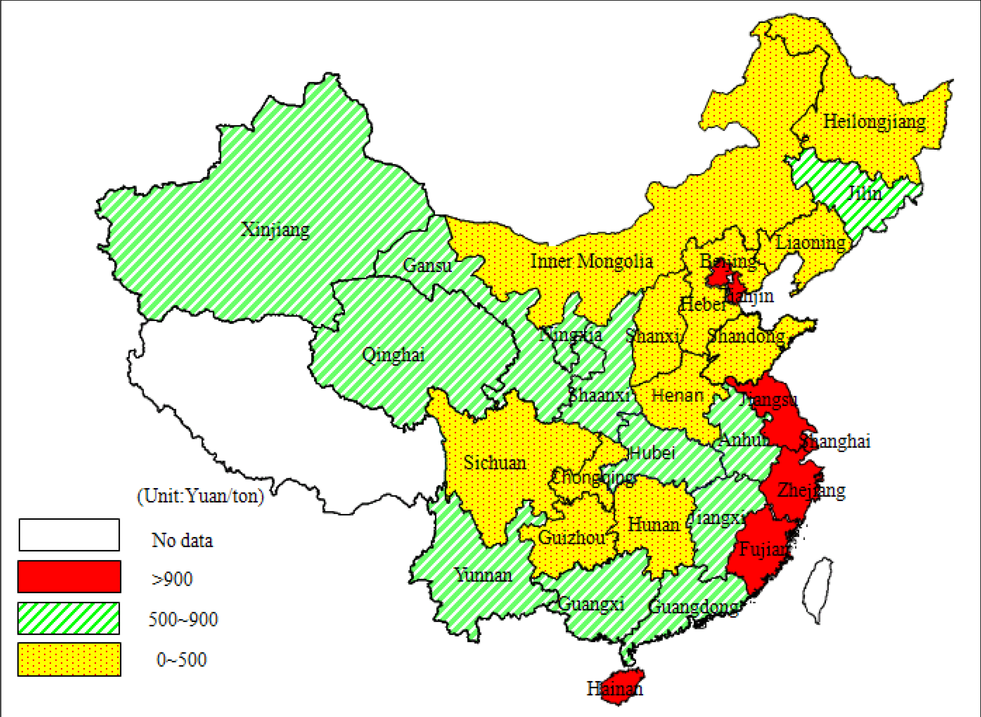
3.3. The Policy Implications for China
4. Conclusions
Acknowledgments
Author Contributions
Conflicts of Interest
References
- Statistical Review of World Energy 2013. Available online: www.bp.com/content/dam/bp/pdf/statistical-review/statistical_review _of_world_energy_2013.pdf (accessed on 19 March 2014).
- Gollop, F.M.; Roberts, M.J. Cost-minimizing regulation of sulfur emissions: Regional gains in electric power. Rev. Econ. Stat. 1985, 67, 81–90. [Google Scholar] [CrossRef]
- Shephard, R.W. Theory of Cost and Production Functions; Princeton University Press: Princeton, NJ, USA, 1970. [Google Scholar]
- Lee, J.D.; Park, J.B.; Kim, T.Y. Estimation of the shadow prices of pollutants with production/environment inefficiency taken into account: A nonparametric directional distance function approach. J. Environ. Manag. 2002, 64, 365–375. [Google Scholar] [CrossRef]
- Kaneko, S.; Fujii, H.; Sawazu, N.; Fujikura, R. Financial allocation strategy for the regional pollution abatement cost of reducing sulfur dioxide emissions in the thermal power sector in China. Energ. Pol. 2010, 38, 2131–2141. [Google Scholar] [CrossRef]
- Färe, R.; Grosskopf, S.; Lovell, C.A.K.; Yaisawarng, S. Derivation of shadow prices for undesirable outputs: a distance function approach. Rev. Econ. Stat. 1993, 75, 374–380. [Google Scholar] [CrossRef]
- Lee, M. The shadow price of substitutable sulfur in the US electric power plant: A distance function approach. J. Environ. Manag. 2005, 77, 104–110. [Google Scholar] [CrossRef]
- Hu, J.L.; L, Y.; Chiu, Y.H.; K, T.Y. Shadow prices of SO2 abatements for regions in China. Agr. Resour. Econ. 2008, 5, 59–78. [Google Scholar]
- Hailu, A. Pollution abatement and productivity performance of regional Canadian pulp and paper industries. J. Forest Econ. 2003, 9, 5–25. [Google Scholar] [CrossRef]
- Murty, M.N.; Kumar, S.; Paul, M. Environmental regulation, productive efficiency and cost of pollution abatement: A case study of the sugar industry in India. J. Environ. Manag. 2006, 79, 1–9. [Google Scholar] [CrossRef]
- Chambers, R.G.; Chung, Y.; Färe, R. Profit, directional distance functions, and Nerlovian efficiency. J. Optim. Theor. Appl. 1998, 98, 351–364. [Google Scholar] [CrossRef]
- Färe, R.; Grosskopf, S.; Noh, D.W.; Weber, W. Characteristics of a polluting technology: Theory and practice. J. Econ. 2005, 126, 469–492. [Google Scholar] [CrossRef]
- Färe, R.; Grosskopf, S.; Weber, W.L. Shadow prices and pollution costs in U.S. agriculture. Ecol. Econ. 2006, 56, 89–103. [Google Scholar] [CrossRef]
- Vardanyan, M.; Noh, D.W. Approximating pollution abatement costs via alternative specifications of a multi-output production technology: A case of the US electric utility industry. J. Environ. Manag. 2006, 80, 177–190. [Google Scholar] [CrossRef]
- Matsushita, K.; Yamane, F. Pollution from the electric power sector in Japan and efficient pollution reduction. Energ. Econ. 2012, 34, 1124–1130. [Google Scholar] [CrossRef]
- Wang, Q.W.; Cui, Q.J.; Zhou, D.Q.; Wang, S.S. Marginal abatement costs of carbon dioxide in China: A nonparametric analysis. Energ. Procedia 2011, 5, 2316–2320. [Google Scholar] [CrossRef]
- Choi, Y.; Zhang, N.; Zhou, P. Efficiency and abatement costs of energy-related CO2 emissions in China: A slacks-based efficiency measure. Appl. Energ. 2012, 98, 198–208. [Google Scholar] [CrossRef]
- Yuan, P.; Liang, W.B.; Cheng, S. The marginal abatement costs of CO2 in Chinese industrial sectors. Energy Procedia 2011, 14, 1792–1797. [Google Scholar]
- Lee, M.; Zhang, N. Technical efficiency, shadow price of carbon dioxide emissions, and substitutability for energy in the Chinese manufacturing industries. Energ. Econ. 2012, 34, 1492–1497. [Google Scholar] [CrossRef]
- Kwon, O.S.; Yun, W.C. Estimation of the marginal abatement costs of airborne pollutants in Korea’s power generation sector. Energ. Econ. 1999, 21, 547–560. [Google Scholar] [CrossRef]
- Hu, J.L.; Kao, C.H. Efficient energy-saving targets for APEC economies. Energ. Pol. 2007, 35, 373–382. [Google Scholar] [CrossRef]
- Zhang, X.P.; Tan, Y.K.; Tan, Q.L.; Yuan, J.H. Decomposition of aggregate CO2 emissions within a joint production framework. Energ. Econ. 2012, 34, 1088–1097. [Google Scholar] [CrossRef]
- Wu, Y. Openness, productivity and growth in the APEC economies. Empir. Econ. 2004, 29, 593–604. [Google Scholar]
- Sun, H.; Zhi, D.L. Estimate of capital stock of provinces in China and the typical fact from 1978 to 2008. J. Financ. Econ. 2010, 25, 107–115. [Google Scholar]
- National Bureau of Statistics of China. China Energy Statistical Yearbook; China Statistics Press: Beijing, China, 2012. (In Chinese)
- National Bureau of Statistics of China (NBSC). China Statistical Yearbook. 2013. Available online: http://www.stats.gov.cn/tjsj/ndsj (accessed on 7 January 2014). (In Chinese)
- Aigner, D.J.; Chu, S.F. On estimating the industry production function. Am. Econ. Rev. 1968, 58, 826–839. [Google Scholar]
- Wei, C.; Ni, J.; Du, L. Regional allocation of carbon dioxide abatement in China. China Econ. Rev. 2012, 23, 552–565. [Google Scholar] [CrossRef]
- Du, L.; Wei, C.; Cai, S. Economic development and carbon dioxide emissions in China: Provincial panel data analysis. China Econ. Rev. 2012, 23, 371–384. [Google Scholar] [CrossRef]
- Wei, Z.X.; Li, W.J.; Wang, T. The impacts and countermeasures of levying carbon tax in China under low-carbon economy. Energy Procedia 2011, 5, 1968–1973. [Google Scholar] [CrossRef]
- Heinonen, J.; Junnila, S. A carbon consumption comparison of rural and urban lifestyles. Sustainability 2011, 3, 1234–1249. [Google Scholar] [CrossRef]
© 2014 by the authors; licensee MDPI, Basel, Switzerland. This article is an open access article distributed under the terms and conditions of the Creative Commons Attribution license (http://creativecommons.org/licenses/by/3.0/).
Share and Cite
Wang, J.; Li, L.; Zhang, F.; Xu, Q. Carbon Emissions Abatement Cost in China: Provincial Panel Data Analysis. Sustainability 2014, 6, 2584-2600. https://doi.org/10.3390/su6052584
Wang J, Li L, Zhang F, Xu Q. Carbon Emissions Abatement Cost in China: Provincial Panel Data Analysis. Sustainability. 2014; 6(5):2584-2600. https://doi.org/10.3390/su6052584
Chicago/Turabian StyleWang, Jianjun, Li Li, Fan Zhang, and Qiannan Xu. 2014. "Carbon Emissions Abatement Cost in China: Provincial Panel Data Analysis" Sustainability 6, no. 5: 2584-2600. https://doi.org/10.3390/su6052584