Article

Towards Life Cycle Sustainability Assessment of Alternative Passenger Vehicles

1
Department of Civil, Environmental, and Construction Engineering, University of Central Florida, Orlando, FL 32816, USA
2
Department of Industrial Engineering, Istanbul Sehir University, Istanbul 34662, Turkey
*
Author to whom correspondence should be addressed.
Sustainability 2014, 6(12), 9305-9342; https://doi.org/10.3390/su6129305
Submission received: 23 October 2014 / Revised: 2 December 2014 / Accepted: 5 December 2014 / Published: 16 December 2014
(This article belongs to the Special Issue Transportation and Sustainability)

Abstract

:
Sustainable transportation and mobility are key components and central to sustainable development. This research aims to reveal the macro-level social, economic, and environmental impacts of alternative vehicle technologies in the U.S. The studied vehicle technologies are conventional gasoline, hybrid, plug-in hybrid with four different all-electric ranges, and full battery electric vehicles (BEV). In total, 19 macro level sustainability indicators are quantified for a scenario in which electric vehicles are charged through the existing U.S. power grid with no additional infrastructure, and an extreme scenario in which electric vehicles are fully charged with solar charging stations. The analysis covers all life cycle phases from the material extraction, processing, manufacturing, and operation phases to the end-of-life phases of vehicles and batteries. Results of this analysis revealed that the manufacturing phase is the most influential phase in terms of socio-economic impacts compared to other life cycle phases, whereas operation phase is the most dominant phase in the terms of environmental impacts and some of the socio-economic impacts such as human health and economic cost of emissions. Electric vehicles have less air pollution cost and human health impacts compared to conventional gasoline vehicles. The economic cost of emissions and human health impact reduction potential can be up to 45% and 35%, respectively, if electric vehicles are charged through solar charging stations. Electric vehicles have potential to generate income for low and medium skilled workers in the U.S. In addition to quantified sustainability indicators, some sustainability metrics were developed to compare relative sustainability performance alternative passenger vehicles. BEV has the lowest greenhouse gas emissions and ecological land footprint per $ of its contribution to the U.S. GDP, and has the lowest ecological footprint per unit of its energy consumption. The only sustainability metrics that does not favor the BEV is the water-energy ratio, where the conventional gasoline vehicle performed best.

1. Introduction

Sustainable transportation and mobility are key components and central to sustainable development. The transportation sector is also an integrated component of the economy and of society as a whole, as it is connected to almost all of the sectors that constitute the entire economy. Especially, concerns associated with global climate change, energy security, rising oil prices, and depletion of fossil fuels are stimulating the search for alternative vehicle technologies. Hybrid electric vehicles (HEV), plug-in hybrid electric vehicles (PHEV), and battery electric vehicles (BEV) are some of these alternative vehicle technologies, which can help to address the aforementioned issues by shifting transportation energy sources use from fossil fuels to electricity, under low carbon electricity generation scenarios [1,2].
In the United States, there are various efforts to increase adoption of these alternative vehicle technologies due to their great potential of reducing fossil fuel consumption and GHG emissions. The U.S. road system has the largest network size in the world, as well as one of the largest network usage densities at three million Vehicle Miles Traveled (VMT) per year. These factors make the U.S. transportation sector an important source of GHG emissions and energy consumption with 28% of the nation’s total emissions [3]. Additionally, the transportation sector consumes immense amounts of petroleum and it is responsible for 67% of the total U.S. petroleum consumption. This high petroleum demand is more than the U.S. petroleum production (141% of total petroleum production in the U.S.), which compromises national energy security and result in high dependency on fossil fuels [4]. Although the alternative vehicle technologies have great potential to minimize the negative economic, social, and environmental impacts of the fast-growing transportation sector, there are certain challenges against widespread adoption of these technologies. These barriers include lack of infrastructure, customer’s unwillingness to purchase these vehicles, high initial costs of BEVs, and insufficient all-electric range [5]. In this regard, national agencies, state level authorities, and international organizations support the adoption of alternative vehicle technologies to increase their market penetration [6,7,8,9,10]. For instance, The Obama administration and the Department of Energy (DOE) aim to reach one million electric vehicles (including HEVs, PHEVs, and BEVs) by 2015 and are trying to accelerate sales by state and federal level incentives [10]. In addition, a program by the DOE, EV-Everywhere Challenge, aims to promote development and research activities to reduce battery costs, increase the all-electric range of electric vehicles, and make these vehicles affordable for American families [11]. While all of these efforts are necessary and useful, it is more important to understand the macro-level social, economic, and environmental (termed as the triple bottom line) impacts of alternative vehicle technologies to be able to develop more effective policies and guide the offering of incentives to the right domains.
Analysis of alternative vehicle systems needs a holistic triple bottom line sustainability accounting which requires a broad set of environmental, economic and environmental indicators [12]. Although many studies have used life-cycle based approaches to quantify the environmental consequences of alternative transportation systems, only a handful of studies have been found in the literature which analyze the socio-economic aspects of these transportation systems. The majority of the studies which conducted an environmental life-cycle assessment of conventional and electric vehicles mainly focused on the limited environmental impact categories such as greenhouse gas emissions, energy consumption, and some mid-point indicators [1,13,14]. In general, the difficulties related to precisely assessing the broader social and economic impacts of transportation stem from lack of appropriate methods, tools and data availability. However, the socio-economic effects of transportation should be considered since they are highly critical for the quality of people’s lives [15]. According to a comprehensive guidebook published by the Transportation Research Board on the socio-economic effects of transportation projects, travel time, safety, vehicle operating cost, noise, and congestion are listed among the prominent socio-economic metrics [16]. In another study related to issues in sustainable transportation, the importance of environmental, economic, and social indicators for sustainability assessment of transportation systems was discussed. According to Litman and Burwell [15], income, employment, accessibility, safety, equity, and affordability are listed as the major socio-economic metrics of sustainable transportation. Offer et al. [17] also conducted a comparative study and focused on the economic impacts of battery and electric vehicles using a life-cycle cost analysis based on capital cost, running cost, and end-of-life cost. Stone et al. [18] used the Global Trade Analysis Project (GTAP) database in order to analyze the socio-economic impacts of transportation projects considering a wide range of socio-economic indicators such as contribution to gross domestic product (GDP), household income, poverty, and import. The World Bank’s report on social analysis of transportation projects also revealed important insights regarding the significance of socio-economic aspects of transportation. In this report, employment, road safety, health impacts, and accessibility are considered key drivers of socio-economic sustainability in transportation [19]. In a report published by the European Commission for the future of sustainable transportation in European States, number of fatalities and injuries, contribution to GDP, employment, external cost of transportation activities such as congestion, emission and safety, taxation, average passenger travel time, and affordability are listed among the key indicators to assess the socio-economic sustainability aspects of transportation activities [20]. As can be seen from the aforementioned review studies and government reports, the selection of socio-economic indicators show differences between the studies; however, economic cost of emissions, income and employment generation, tax, human health impacts, contribution to GDP and foreign trade can be seen as commonly used quantitative indicators that are addressed in this research. Other indicators such as accessibility, affordability, equity, travel time, congestion and noise are excluded from the scope of this paper due to lack of appropriate data for new electric vehicle technologies, irrelevance to the aim of this paper, and difficulties in integration with a proposed input-output based life cycle approach.

1.1. Life Cycle Assessment

Life Cycle Assessment (LCA) is a well-known and widely-used approach used to quantify environmental impacts related to the life cycle of products, including raw material extraction, manufacturing, transportation, use, and final disposal [21]. LCA was introduced in the early 1990s as a practical and robust tool to assess and reduce the potential environmental loads of industrial activities [22]. One of the most prominent strengths of LCA is to consider the whole product life cycle so as to avoid problems associated with working with a limited scope. In the literature, three LCA approaches have been used in many studies: process-based LCA (P-LCA), input-output based LCA (IO-LCA), and hybrid LCA which is the combination of the P-LCA and IO-LCA [23,24]. P-LCA divides the product’s manufacturing process into individual process flows to quantify the related direct environmental impacts, providing a methodological framework to estimate the environmental impacts of specific processes [25,26]. Among the LCA methodologies, P-LCA has been often used to analyze the environmental impacts of certain phases such as manufacturing, transportation, use and end-of-life without looking at the supply chain components. Thus, due to the narrowly defined system boundaries, some important environmental impacts in the extended supply chains might be overlooked by the P-LCA method since it is not possible to include all of the upstream suppliers for impact assessment [27]. To overcome these limitations, IO-LCA models were initiated as robust methods in the early 2000s [28]. The IO-LCA, which is widely used in literature for quantifying the environmental impacts of products or processes, is capable of covering the entire supply chain when quantifying the overall environmental impacts.

1.2. Input-Output Based LCA

When working with large-scale systems such as manufacturing or transportation, IO-LCA models can be the better approach, as they provide an economy-wide analysis [29]. On the other hand, process-based analysis involves a limited number of processes, and the inclusion or exclusion of processes is decided on the basis of subjective choices, thereby creating a system boundary problem [23]. Earlier studies on the direct and indirect carbon and energy footprint analysis of different economic sectors also showed that P-LCA suffers from significant truncation errors which can be in the order of 50% or higher [30,31,32]. Therefore, the I-O based LCA models provide a top-down analysis using sectorial monetary transaction matrixes considering complex interactions between the sectors of nations’ economy [33]. The I-O technique is a suitable approach for calculation of environmental footprints [28].
Using the Economic Input-Output LCA (EIO-LCA) model, an I-O based LCA model, Matthews et al. [32] analyzed the carbon footprints of different industrial sectors and the results of this study revealed that, on average, direct emissions from an industry account for only 14 percent of the total supply chain carbon emissions. Additionally, direct emissions plus industry energy inputs were found to be only 26 percent of the total supply chain-linked emissions. Therefore, using a comprehensive environmental LCA method like IO-LCA is vital for tracking total environmental pressures across the entire supply chain network. As employed in this research, Hybrid LCA combines both the P-LCA and IO-LCA models to analyze process-specific and supply chain-related sustainability impacts. Although IO-LCA was one of the most comprehensive LCA methods developed, due to its limited focus on only the environmental impacts, a new IO-LCA model needs to be developed to cover triple bottom line (TBL) impacts and provide a more robust analytical framework, which can be used to conduct broader LCA’s of products or systems [34,35].

1.3. The State-of-the-Art: Life Cycle Sustainability Assessment

Over the last decade, there has been a transition from LCA to Life Cycle Sustainability Assessment (LCSA), in which environmental, economic, and social dimensions of sustainability are integrated into a traditional LCA methodology [36,37,38]. According to a recent article on the past, present and future of LCA, the period between 2010 and 2020 is known as the “decade of life cycle sustainability assessment” [39]. The United Nations Environment Programme (UNEP) and the Society of Environmental Toxicology and Chemistry (SETAC) have been working on possible methodological approaches and metrics in order to fully integrate triple bottom line aspects of sustainability into a single-dimensioned LCSA [40]. In this framework, environmental LCA, life cycle cost (LCC), and social life cycle assessment (S-LCA) represent three independent methodologies to individually address the three pillars of sustainability [41].
In the literature, Kloepffer [42] first formulated the current LCSA framework with editorial comments obtained from Finkbeiner and Reiner, where the “LCSA = LCA + LCC + S-LCA” [43]. According to a report by UNEP & SETAC, although there has been little progress toward improving the methodological aspects that extend the application areas for LCSA, LCSA is certainly an important framework and should be pursued [44].
LCSA is still a new concept, and the applications of this method in sustainability assessment research are highly limited. After a comprehensive review of authors, there are a limited number of studies found in the literature that have used LCSA in a real case study for product LCSA, and the majority of those papers focused mainly on the methodological or conceptual aspects of LCSA. Hu et al. [45] presented an approach to put the LCSA framework into practice by analyzing the triple bottom line life cycle implications of concrete recycling processes. In another paper, Traverso et al. [46] analyzed the production steps of photovoltaic (PV) modules where environmental, economic and social impacts of Italian and German polycrystalline silicon modules are compared using LCSA. Although several studies emphasized the importance of system-based tools for LCA, the applications of LCSA for large systems are also missing. Guinée et al. [39] highlighted the importance of the LCSA framework in future LCA and discussed the necessity of system-based sustainability accounting methods such as IO LCA and hybrid LCA. Wood and Hertwich [47] also discussed the comprehensiveness of I-O analysis in LCSA, particularly for socio-economic analysis. In response to the current research needs regarding comprehensive LCSA methods, Kucukvar et al. [3] developed an optimization model in which input-output based LCSA and compromise programming methods are used in conjunction for a multi-criteria decision analysis of hot-mix and warm-mix asphalt mixtures. In a recent work, Onat et al. [34] used the LCSA framework for a TBL sustainability analysis of U.S residential and commercial buildings and demonstrated the usefulness of input–output modeling to quantify sustainability impacts as integration into the LCSA framework.

1.4. Research Objectives Against the Background of the State-of-the-Art

Combined applications of LCSA and input-output analysis are very limited in the literature [34]. Although the literature is abundant with studies focusing on environmental impacts of alternative vehicle technologies [1,2,13,48,49,50,51], the social and economic dimensions of adoption of these vehicle technologies were not investigated sufficiently. Moreover, studies covering economic dimensions are mostly limited to life cycle cost analyses and do not investigate the economy-wide impacts of alternative vehicle technologies. Considering that the fundamental concept of sustainability encompasses issues related to economy, environment, and society as a whole, studies analyzing issues related to the adoption of alternative passenger vehicles should not focus on only environmental or economic aspects, but should instead evaluate alternatives considering their triple bottom line (TBL) impacts all together.
In this regard, this research aims to advance the LCSA literature and electric vehicles’ sustainability research by filling two major knowledge gaps: “lack of integration of I-O analysis for LCSA” and “lack of quantified macro-level TBL impacts of electric vehicles”. Furthermore, the LCA literature on sustainability analysis of alternative vehicle technologies needs a holistic LCSA analysis in which both direct and supply-chain-related indirect triple bottom line sustainability implications of vehicles are analyzed. With this motivation in mind, this research will utilize a holistic I-O technique for supply chain-linked LCSA of alternative electric vehicle technologies in the U.S. In this study, the following objectives were set forth: (1) to quantify economic, social, and environmental impacts of alternative passenger vehicles; (2) to compare these alternatives and evaluate their macro-level sustainability impacts; (3) to show how cleaner charging options affect the TBL performance of alternative vehicle technologies, and 4) to compare TBL impacts of the manufacturing, operation, and end-of-life phases of various alternative vehicle technologies.

2. Methods

In this study, life cycle assessment and economic input-output analysis are utilized, which are explained in detail in the following sections. First, the scope of the analysis is represented, and the system boundary is defined. Second, TBL indicators are introduced as measurements of sustainability, and their calculation steps are briefly explained. Third, data sources and specific calculations associated with each life cycle phase are presented. Fourth, the results are presented for each sustainability indicator, and the analyzed vehicle alternatives are compared, accordingly. Furthermore, there are two scenarios considered in this analysis: Scenario 1 is based on existing electric power infrastructure in the U.S. with no additional infrastructure requirement, while Scenario 2 is an extreme scenario in which electricity to power BEVs and PHEVs are generated through solar charging stations only.

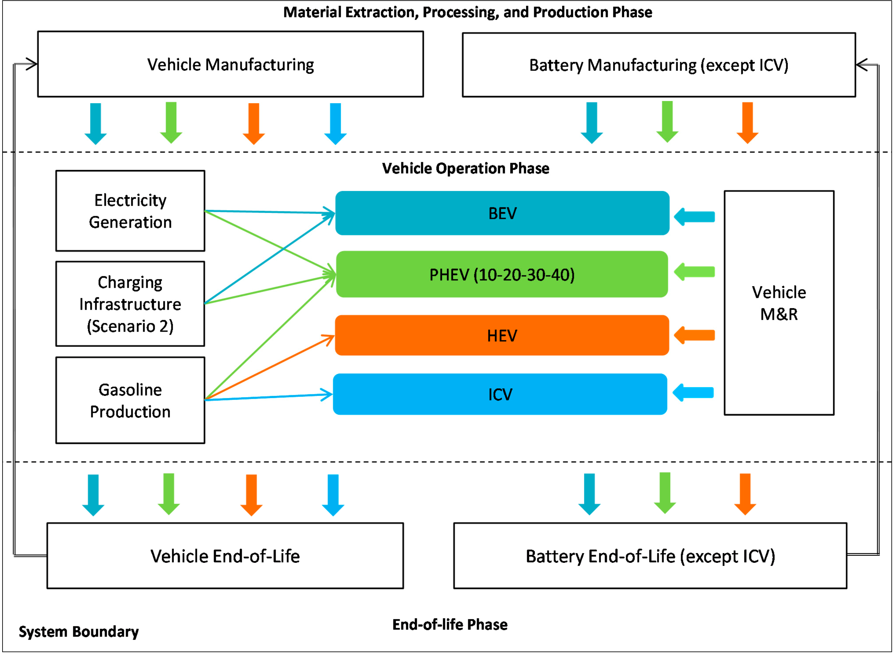
2.1. Scope of the Analysis

This analysis covers all life cycle phases from the material extraction, processing, manufacturing, and operation phases to the end-of-life phases of vehicles and batteries. The system boundary of the analysis is represented in Figure 1. The vehicle technologies are internal combustion vehicles (ICVs), HEVs and PHEVs with all-electric ranges (AER) of 10, 20, 30, and 40 miles of electric powered drive, and BEVs. AER is defined as the total miles can be driven in electric mode (engine-off) with an initially fully charged battery until the internal combustion engine turns on for the first time [52]. All of the battery types utilized in the alternative passenger vehicles are lithium ion (li-ion) batteries. The useful life time for these vehicles is assumed to be 150,000 miles and the functional unit is defined as 1 mile of vehicle travel. Each color in Figure 1 represent one vehicle type and the arrows indicate that there is a relationship between the associated vehicle and the corresponding process. For instance, electricity generation and construction of solar charging stations are the processes that are related to BEVs and PHEVs only. Similarly, the battery manufacturing and end-of-life of batteries are not calculated for the ICVs as they do not utilize li-ion batteries.
Figure 1. System boundary of the analysis.
Sustainability 06 09305 g001

2.2. The TBL-LCA Model and Sustainability Indicators

The TBL-LCA model is an I-O-based sustainability accounting tool, which is utilized to quantify the environmental, economic, and social impacts associated with alternative passenger vehicles. The I-O analysis was introduced by Wassiliy Leontief in the 1970s [53], and since that time, various extensions of this methodology were developed. I-O models are consist of identical sectors and the money flow among these sectors that constitute the whole economy of a country, a region, or the entire world depending on the scope and structure of the data [28,54,55]. Most of the developed countries publish their I-O tables consisting of financial flow data among the defined sectors, in which financial flow data is represented by supply and use tables. The U.S. Bureau of Economic Analysis (BEA), publishes these tables periodically, once in a 5 year period, in which all sectors are classified according to the North American Industry Classification System (NAICS) [56,57]. Environmentally-extended I-O (EEIO) models such as the Economic Input-Output LCA (the EIO-LCA) [58] and the Ecologically-based LCA (Eco-LCA) [59] incorporate the financial flow data from the supply and use tables with environmental impact factors reflecting the environmental impacts of the sectors per commodity output in the terms of monetary units. In addition to environmental indicators, the TBL-LCA model incorporates social and economic indicators and presents an I-O based holistic sustainability accounting framework. In the TBL-LCA model, an industry-by-industry I-O methodology was utilized, which was also used in previous I-O based TBL models developed for economies of the UK and Australia [60,61]. Also, the conversion of supply and use tables into an industry-by-industry I-O table is conducted based on the fixed industry sales assumptions. For more detailed information about the transformation of supply and use tables, please see the reference reports published by the Eurostat [62] and by the United Nations [63].
In the TBL-LCA model, the I-O multipliers represent the total impacts, which are accumulations of direct and indirect (supply chain) impacts per unit of final demand of commodities produced by the NAICS sectors. The monetary transactions between the sectors are represented as a set of matrices. The Use matrix, mostly denoted as U, represents the financial flow due to the consumption of commodities by sectors. While the columns represent the commodities, the sectors using those commodities are placed in rows. For example, the monetary value of steel consumption of the automobile manufacturing sector is in the intersection of the steel manufacturing sector in the row and automobile manufacturing sector in the column. The Make (supply) matrix, usually denoted as V, shows the production of commodities by each sector. In the Make matrix, the columns and rows represent the commodities and sectors, respectively. However, the intersections of the rows and columns represent the production of the commodity by the sector in the row [64].
=   [ b ij ] = [ U ij X j ]
=   [ d ij ]   =   [ V ij q i ]
In Equations (1) and (2), the Use and Make matrices are expressed with the technical coefficient matrices B and D, respectively. As a part of the U matrix, uij stands for the monetary value of the purchase of commodity i by sector j, while Xj is the total output of sector j. Hence, bij is the amount of commodity i needed for generating one dollar output of sector j. On the other hand, vij represents the monetary value of the output of commodity i by sector j and qi is the output of commodity i. Therefore, dij is the fraction of total output of commodity i that is produced by the sectors. Equation (3) is the total impact vector which indicates the total sustainability impacts per unit of final demand [64].
= E dir [ ( I DB ) 1 ] f
In Equation (3), I represents the identity matrix and f represents the final demand vector of industries. Also, the formulation [(I-DB)−1] represents the total requirement matrix, which is also known as the Leontief inverse [53]. Edir is a diagonal matrix consisting of the triple bottom line impact values per dollar output of each sector.
Table 1. Brief description of sustainability indicators.
Bottom LinesTBL IndicatorUnitDescription
EnvironmentalGlobal Warming Potential (GWP)gCO2-eqv.The total GHG emissions based on IPPC’s values for GWP100.
Water WithdrawalltThe total amount of water withdrawals of each sector.
Energy ConsumptionMJThe total energy consumption of industries.
Hazardous Waste GenerationstThe amount of hazardous waste (EPA’s RCRA) generated by U.S. sectors
Particulate Matter Formation Potential (PMFP)gPM10-eqv.The total criteria air pollutant emissions based on ReCiPe CFs.
FisheryghaThe estimated primary production required to support the fish caught.
GrazingghaThe amount of livestock feed available in a country with the amount of feed required for the livestock produced.
ForestryghaThe amount of lumber, pulp, timber products, and fuel wood consumed by each U.S. sector.
CroplandghaThe most bio-productive of all the land use types and includes areas used to produce food and fiber for human consumption.
CO2 uptake landghaThe amount of forestland required to sequester GHG emitted by sectors.
EconomicImport (foreign purchase)$The monetary value of products and services purchased from foreign countries to produce domestic commodities.
Gross Operating Surplus (business profit)$The available capital of corporations, which allows them to pay taxes, to repay their creditors, and to finance their investments.
Gross Domestic Product (GDP)$Economic value added by the U.S. sectors.
Air emission cost$Economic costs of externality damages due to releases of CO, nitrogen oxides (NOx), particulate matter (PM), SO2, volatile organic compounds (VOCs), and GHGs.
SocialEmploymentemp-hThe full-time equivalent employment hours for each U.S. sector.
Government Tax$Taxes collected from production and imports, government revenues.
Injuries#workerThe number of non-fatal injuries associated with the U.S. sectors.
Income$The compensation of employees, wages, and salaries.
Human HealthDALYThe number of years lost due to disability, illness, or early death.
In this study, 16 macro-level indicators were selected to represent environmental, economic, and social impacts. Table 1 shows the selected indicators and their brief definitions. These indicators are utilized as multipliers (impact per $M of output) to quantify impacts associated with each activity. Data required to calculate these multipliers was obtained via publicly available resources such as the Bureau of Economic Analysis [56], the Bureau of Labor Statistics [65], the Global Footprint Network [66], and Carnegie Mellon’s EIO-LCA software [58]. For more detailed information about the TBL-LCA model and the sustainability indicators, please see the reference study published by Kucukvar and Tatari [30]. The selection of social criteria in sustainable transportation research and their quantification are still some of the major challenges when implementing the complete triple-bottom-line sustainability analysis. There are still research needs for social LCA and there is no standard usage of a predetermined set of social indicators worldwide [43,44]. However, in accordance with the literature review on indicators for sustainable transportation, issues in data availability, and ease of integration with current LCSA methodology, the authors selected the following socio-economic indicators that are presented as:
Income, in other words compensation of employees, is chosen as a positive social indicator since it contributes to the social welfare of households. This indicator represents the compensation of employees, including wages and salaries [15,67]. The total income generated by each sector is obtained from the input-output accounts published by the U.S. Bureau of Economic Analysis [56]. Using the World Input-Output Database supported by the European Commission under the th research programme, the total income is presented in terms of three skill groups such as low-skilled, medium skilled and high-skilled [68]. The WIOD database used the 1997 International Standard Classification of Education classification to define low, medium, and high skilled labors which are defined in Table 2.
Table 2. Summary of skills in World Input-Output Database (WIOD) [69].
WIOD Skill-TypeISCED LevelISCED Level Description
Low1Primary education or first stage of basic education
Low2Lower secondary or second stage of basic education
Medium3(Upper) secondary education
Medium4Post-secondary non-tertiary education
High5First stage of tertiary education
High6Second stage of tertiary education
Employment is selected as positive social indicator and represents the full-time equivalent employment hours for each U.S. sector [70]. The values of total employment hours of each sector are obtained from the U.S. Burea of Labour Statistics Database [65].
A work-related injury represents the negative social indicator and is the total number of non-fatal injuries at each of 426 sector of U.S economy. The data including the number of total work place injuries are obtained from the U.S. Bureau of Labor Statistics to analyze the contributions of the each sector to work-related non-fatal injuries [28,65].
Human health is selected as an end-point social indicator which is originally developed by Harvard University and adopted by the World Health Organization. Impact to human health is presented as disability-adjusted life year (DALY) which is the number of years lost due to disability, illness, or early death as a result of environmental impacts [71]. The human health impacts are quantified in accordance with the characterization factors (CFs) provided ReCiPe which is a well-known Life Cycle Impact Assessment (LCIA) methodology [72]. In this study, DALY is determined by the impacts of particulate matter formation (PMF), photochemical oxidant formation (POF), and global warming potential (GWP), which are three common environmental mid-point indicators. Considering that the value choices influence the analysis of human health damages in LCA, there are different way of quantifying these impacts based on the value choices, which are egalitarian, hierarchist, and individualist [73,74,75]. The quantified human health impacts are based on hierarchist perspective since it is more suitable for macro-level impact assessment than other value choices [74,76].
Air emission cost is presented as life cycle emission cost of alternative vehicle technologies, which includes the location-specific externality damages for releases of CO, nitrogen oxides (NOx), particulate matter (PM), SO2, volatile organic compounds (VOCs), and GHGs. The location-specific emission costs data is obtained from a comprehensive study conducted by Michalek et al. [77], in which the air pollution costs associated with environmental impact, mortality, and morbidity is included. GHG cost estimates includes net agricultural productivity, human health, property damages from increased flood risk, and the value of ecosystem services due to climate change [77,78]. These costs are based on National Resource Council (NRC) study, literature survey and estimates from the US Interagency Working Group on Social Cost of Carbon. In this study, we used, $9.66 per metric tons of CO2-eqv., which is 23% of the medium-level global damage value of Climate change, recommended by the Interagency Working Group [79].
Taxes are chosen as a positive sustainability indicator since collected taxes will be used for supporting the nation’s prosperity through investments on health and education systems, transportation, highways, and other civil infrastructures [60,80]. Taxes are also referred to as government revenue, which accounts for the taxes on production and imports. The data source for taxes generated by each sector is the U.S. input–output tables [56].
Profit, in other words gross operating surplus (GOS), is the residual for industries after subtracting total intermediate inputs, compensation of employees, and taxes from total industry output [62]. Profit is considered as a positive economic indicator since it represents the capital available to sectors, which allow them to pay taxes and to finance their investments.
Gross Domestic Product (GDP) is used as another macro-level economic indicator. GDP typically represents the market value of goods and services produced within the country in a given period of time. GDP is a positive economic indicator that monitors the health of a nation’s economy and includes compensation of employees, gross operating surplus, and net taxes on production and imports [64]. This positive economic indicator is the direct and indirect contribution of one sector to GDP.
Imports, in other words foreign purchases, represent the value of goods and services purchased from foreign countries to produce domestic commodities by industries [67]. This economic indicator accounts for the direct and indirect contributions of one sector to foreign purchases. The import value of each sector is obtained from the U.S. input–output tables [56].
Although a majority of the LCA analysis is conducted with the industrial TBL multipliers, there are some processes which are not represented by the sectors in the model. In these cases, process impacts are calculated manually. For instance, the driving activity within the operation phase of vehicles cannot be represented by any of the 428 sectors. In this case, the amount of fuel consumed is calculated and multiplied by the relevant factor, such as CO2 emissions from burning one gallon of gasoline. This approach is termed as tiered hybrid I-O analysis in the literature [23]. Similar approaches can be also found in [28]. A detailed explanation of these calculations will be presented in the following section.

2.3. Life Cycle Inventory

Vehicle features such as weight, battery power requirements, and material compositions are obtained from the Greenhouse Gases, Regulated Emissions, and Energy Use in Transportation (GREET) vehicle cycle model [81]. Direct and indirect impacts of activities such as automobile and battery manufacturing, electric power generation, gasoline supply, and savings due to recycled batteries and vehicles are calculated via the TBL-LCA model. First, the monetary values (producer prices) of each process, material, or activity are calculated based on the defined functional unit, which represent the estimated demand from associated sectors as a result of a certain process, such as the amount of fuel required for an ICV to travel 1 mile. These monetary values are inputs for the TBL-LCA model, and are multiplied by the corresponding sector’s TBL multipliers. On the other hand, direct impacts such as tailpipe emissions and direct energy consumption while driving are calculated using process level data. Table 3 lists each activity or process along with a brief description and the corresponding NAICS sector. TBL impact multipliers per $M output of each sector are provided in Table 4. Additionally, emissions of CO, PM2.5, PM10, VOC, NOx, and SO2 are calculated via using sector level multipliers from the EIO-LCA model [58]. Emissions per burning a gallon of gasoline are obtained from literature [82] and GREET model [83] to account for direct tailpipe emissions during the operation phase of the vehicles. Then, the mid-point indicators as well as human health indicator are calculated using these emission amounts and the characterization factors from ReCiPe [72]. Detailed calculation steps and data sources associated with the vehicle and battery manufacturing, operation, and end-of-life phases are provided in the following subsections.
Table 3. Process descriptions and corresponding NAICS sectors through LCA of vehicles.
LCA PhasesNAICS Sector IDNAICS Sector NameProcess Description
Manufacturing Phase335912Primary Battery ManufacturingLi-ion battery manufacturing for vehicles
336111Automobile manufacturingManufacturing of passenger vehicles
Operation phaseDriving related activities221100Electric power generation, transmission, and distribution
324110Petroleum refineriesGasoline production and supply for vehicles
811100Automotive repair and maintenance, except car washesVehicle repair and maintenance
Solar Charging station const.334413Semiconductor and related device manufacturingManufacturing of solar modules and installed system
327320Ready-mix concrete manufacturingConcrete manufacturing
331110Iron and steel millsSteel Manufacturing
321212Veneer and plywood manufacturingMedium density fibreboard manufacturing
32551Paint and coating manufacturingPaint and coating manufacturing
230101Other Nonresidential (layer 1)Construction of the charging station (layer 1 only)
End-of-Life phase331110Iron and steel millsSavings from recycled steel extracted from vehicles and batteries
33131AAlumina refining and primary aluminum productionSavings from recycled aluminum extracted from vehicles and batteries
331420Copper Rolling, Drawing, Extruding, and AlloyingSavings from recycled copper extracted from vehicles and batteries
327211Flat glass manufacturingSavings from recycled glass extracted from vehicles
325211Plastics material and resin manufacturingSavings from recycled plastic extracted from vehicles
325212Rubber and plastics hose and belting manufacturingSavings from recycled rubber extracted from vehicles
339910Jewelry and Silverware ManufacturingSavings from recycled platinum extracted from vehicles
Table 4. TBL impact multipliers per $M output of each sector.
TBL Indicators
Econ.SocialEnvironmental
LCA PhasesNAICS Sector IDsForeign Purchase (M$)Business Profit (M$)Employment-hrIncome (M$)Government Tax (M$)Injuries (# worker)Fishery (gha),Grazing (gha)Forestry (gha)Cropland (gha)Carbon Fossil Fuel (gha)Carbon Electricity (gha)GHG Total (t)Total Energy (TJ)Water (kgal)Haz. Waste (st)
Man. Ph.3359120.2960.53323,3570.4290.0310.5520.0980.1023.173.9897.6741.73540.408.446682364,000
3361110.9690.37028,4220.5640.0430.8470.1732.7623.739.86100.5142.15547.568.488313416,000
Operation phase2211000.0990.48816,1250.3640.1430.2900.2730.1741.343.881853.9213.088243.8798.22219,474125,000
3241100.8530.54516,0990.3450.1000.3290.1530.1261.734.67492.0757.462776.5231.5785464,120,000
8111000.1010.31437,4230.5940.0760.8650.1870.4111.593.5261.9034.16312.324.745184172,000
3344130.4450.43323,2020.5190.0390.4860.1350.1262.053.4793.3354.59579.077.3677511,080,000
3273200.1060.37332,6220.5760.0441.0360.1890.1521.917.71638.1768.342715.1623.3916,526373,000
3311100.4450.30632,8440.6270.0581.0140.2150.2452.876.14546.56123.693669.3051.0220,2331,450,000
3212120.3630.31939,0620.5960.0821.3570.1851.074498.9529.74145.8568.18747.6816.6917,770183,000
325510.2340.38327,6530.5630.0440.6390.2040.2283.6133.42195.3556.831041.9616.18138,9652,080,000
2301010.0000.08220,9190.4430.0050.6030.0000.0000.008.2948.007.69200.003.162160
End-of-Life phase3311100.4450.30632,8440.6270.0581.0140.2150.2452.876.14546.56123.693669.3051.0220,2331,450,000
33131A0.6760.34931,2030.5740.0630.9160.2330.3013.064.76510.62298.613303.3648.0637,142233,000
3314200.5830.33132,0340.6060.0560.9970.2410.2743.306.68217.0884.17964.6515.9712,935334,000
3272110.2360.42330,1760.5280.0410.9920.1640.1405.445.71443.78105.472044.3637.3016,690320,000
3252110.4310.38425,8250.5370.0660.5100.2470.2773.0255.21435.4594.452398.3140.3324,6325,610,000
3252120.4450.32134,9880.6190.0391.0550.1970.2519.5628.24167.2863.45864.3314.2915,3361,090,000
3399102.3680.30836,6770.6200.0470.9840.1980.1502.293.38115.5946.68738.358.788045240,000
* GDP ($M) multiplier for each sector is equal to 1.00.

2.3.1. Vehicle and Battery Manufacturing

Vehicles and battery components are calculated separately to distinguish between battery and vehicle manufacturing impacts by using two NAICS sectors as presented in Table 4. The bodies of the vehicles were assumed to be identical since the price premium for alternative vehicles such as HEVs, PHEVs, and BEVs over a conventional vehicle primarily stem from the additional battery and electronics. Vehicle bodies considered in this analysis are assumed to be similar to an existing Toyota Corolla. Although there are other factors affecting the price premium such as design and manufacturing cost, the price and impacts of manufacturing a Toyota Corolla are used as a baseline for analyzing the manufacturing impacts of all vehicles. This assumption is consistent with Samaras’s study [2]. After calculating the producer price (assumed to be 80% of the retail price) of a Corolla, this monetary input was multiplied by the associated impact multipliers provided in Table 4. It should be noted that all producer price values used in this analysis were converted to $2002, since the TBL-LCA model uses 2002 as a benchmark year.
In this analysis, the lifetimes of the batteries and vehicles are assumed to be same, and it is also assumed that the batteries are not replaced at any time during the operation phase of each vehicle. In the case of the battery being replaced in the future, the impacts from battery production may not necessarily be doubled, since the battery industry is improving rapidly and the environmental impacts such as GHG emissions and energy consumption might be lower than they are today. Battery weights, specific power, and capacity are derived from the GREET 2.7 vehicle cycle model [81,83], in which the vehicle configurations are calculated using Autonomie software [84,85] developed by the U.S. DOE Energy Vehicle Technologies Program. After the battery weights and specific power requirements are calculated with the GREET 2.7 model, the costs associated with production of these li-ion batteries are derived from Argonne National Laboratory’s cost estimation study for li-ion batteries [86]. Once the manufacturing costs of each battery are obtained, these values are multiplied by the multipliers of the associated NAICS sector provided in Table 4. Battery properties and associated cost values are presented in Table 5.
Table 5. Properties of Li-ion batteries for each vehicle type.
Vehicle TypeBattery Weights (lb)Battery Energy Outputs (kwh)Cost Per Energy Output ($2002/kwh)
ICV0.000
HEV41.228 *36.96 *
PHEV10119.24.0201.94
PHEV20208.57.0201.94
PHEV30387.313.0201.94
PHEV40536.318.0201.94
BEV821.338.0201.94
* The unit for peak battery power for HEV is kW, whereas other values represent the peak battery energy (kWh).
While there are no direct impact calculations for the manufacturing phase, there is a federal tax credit up to $7500 for electric vehicles acquired after 31 December 2009. Hence, the earnings from collected taxes from automobile purchase, the impact category “government tax”, are modified to account for these federal tax credit incentives. The tax credit is equal to $2500 plus an additional $417 for each kilowatt hour of battery capacity in excess of 5 kWh, whereas vehicles are required to have at least 5 kWh of battery capacity, and the maximum amount of the credit allowed for a vehicle is $7500 [87]. Air emission costs ($2010) for vehicle and battery manufacturing are $448, $2577, $4763, $31,966, $12,735, and $2400 per metric tons of CO, NOx, PM10, PM2.5, SO2, and VOC, respectively. [77]. These costs are average damage values of the U.S. counties where vehicle and parts manufacturing occurs.

2.3.2. Operation Phase

In the literature, the operation phase impacts associated with vehicles are calculated in two main stages: “well-to-tank (WTT)” and “tank-to-well (TTW)”. While the former covers upstream impacts such as raw material extraction, fuel production and fuel delivery, the latter refers to direct impacts such as tail pipe emissions and direct energy consumption during the operation of vehicles [85]. WTT impacts are calculated using the sector multipliers of the TBL-LCA model presented in Table 4. The producer price ($) for one gallon of petroleum and/or for one kWh of electricity is then used to calculate per mile fuel costs for each vehicle. Next, the impacts of supplying electricity or gasoline are calculated by multiplying the monetary value of per-mile consumption by the associated sector multiplier. The fuel economy (FE) of ICV and HEV are assumed to be 30 and 50 miles per gallon (mpg), respectively, whereas the FE for PHEVs is assumed to be 50 mpg in gasoline mode and 0.29 kWh/mile in electric mode. FE values of these vehicles are similar to those of the Corolla and Prius models currently available in the market. Also, the FE for EV is assumed to be 0.32 kWh/mile. The electricity required to travel a mile includes regenerative braking benefits as well as efficiency losses in the battery, charger, and electric motor. Although these vehicles are generic, the FE values are similar to their counterparts available in the market except with respect to the PHEV20, PHEV30 and PHEV40 [88,89,90,91,92]. TTW impacts are calculated using data from the U.S. Environmental Protection Agency (EPA), GREET model, ReCiPe, and literature for direct energy consumption, GHG emissions, criteria air pollutants [82,83,93,94]. TTW impacts are calculated only for the indicators of GWP, energy consumption, PMF, human health, and air emission costs since there is no other direct impact according to the selected indicators. Cost per unit amount of emissions is the highest in operation phase considering that driving is placed in denser populated areas than other activities such as manufacturing, power generation, and other upstream activities [77]. All pollutant valuations are based on weighted average of county-specific valuation data provided the Air Pollution Emission Experiments and Policy (APEEP) model which evaluates emissions in each county in the U.S. with its exposure, physical effects, and resulting monetary damages [77]. Also, CO valuation costs are from Matthews et al. [95]. Air emission costs ($2010) for vehicle and battery manufacturing are $886, $3445, $11,644, $75,850, $25,512 and $2400 per metric tons of CO, NOx, PM10, PM2.5, SO2, and VOC, respectively. For further information about the methodology for valuation of air emissions please see Michalek et al. [77].
A different calculation method is used for the PHEVs, since they use both electricity and gasoline. The portion driven with electricity is determined by utility factors (UF) for each PHEV. To calculate UFs, the national daily cumulative VMT distribution is constructed, which indicates the percentage of cumulative daily VMT less than a given distance per day. As the main objective is to estimate what percentage of daily travel can be powered by PHEV, their AER features determine this percentage. For instance, vehicles traveling less than 30 miles per day compromise approximately 63% of the daily VMT in the U.S. [96], which means that the UF of PHEV30 is 0.63. The UFs for each PHEV are calculated based on the data obtained from 2009 National Household Travel Survey (NHTS) [97]. Through these calculations, the UFs for PHEV10, PHEV20, PHEV30, and PHEV40 are found to be 0.29, 0.5, 0.63, and 0.71, respectively. Hence, the total impacts for PHEVs can be calculated as follows:
( Impacts per mile ) i =  UF ×   ( FE Elct . × ( WTT impacts Power generation ) i + ( TTW impacts ) i ) +   ( 1 UF ) × ( 1 FE gasoline × ( WTT impacts gasoline production ) i + ( TTW impacts ) i )
where I = Different TBL indicators. In Equation (4), the first part of the equation represents the impacts associated with electricity consumption, while the second part represents impacts associated with the gasoline driven mode. For the EV, the UF is equal to 1. When calculating the impacts of ICV and HEV, only the second portion of the equation is used since they use only gasoline. In other words, the UF for HEV and ICV are both equal to 0.
For Scenario 2, the electricity to power the EVs and the electric mode portion of the PHEVs are generated exclusively through solar charging stations. Therefore, the impacts associated with the construction of a solar charging station are also quantified. Data for solar charging station including materials and installed capacity of the power system are obtained from the literature [98]. First, the amounts and corresponding monetary values for the materials are determined, and these are then multiplied by the associated sector multipliers provided in Table 4 to calculate TBL impacts such as the energy required to produce those materials. The first layer of the NAICS sector, “Other Nonresidential Construction”, is used to calculate the impacts from the construction of the solar charging station. The total TBL impacts are then divided by the estimated total power generation to calculate impact per kWh of electricity generation. The solar charging station is also assumed to be connected to the grid, and therefore transfers the electricity to the grid when it is not charging any vehicles [98].
Another component of the operation phase to consider is the maintenance and repair (M&R) of the vehicles. The M&R costs are obtained from the U.S. Transportation Energy Data book [99]. The M&R costs for an EV and a PHEV are approximately 65%–80% of the M&R cost of an ICV, owing to fewer moving parts and components as well as lower maintenance requirements for electric motors in EVs [100,101]. In this analysis, the M&R costs of PHEVs are assumed to be 80% of those of the ICV, whereas M&R costs of the EV are assumed to be 70% of the ICV, and the cost for the HEV is assumed to be same as those for the ICV [100]. After the M&R costs are determined for each vehicle, these monetary values are multiplied by the TBL multipliers of the associated sectors as provided in Table 4.

2.3.3. End-of-Life Phase
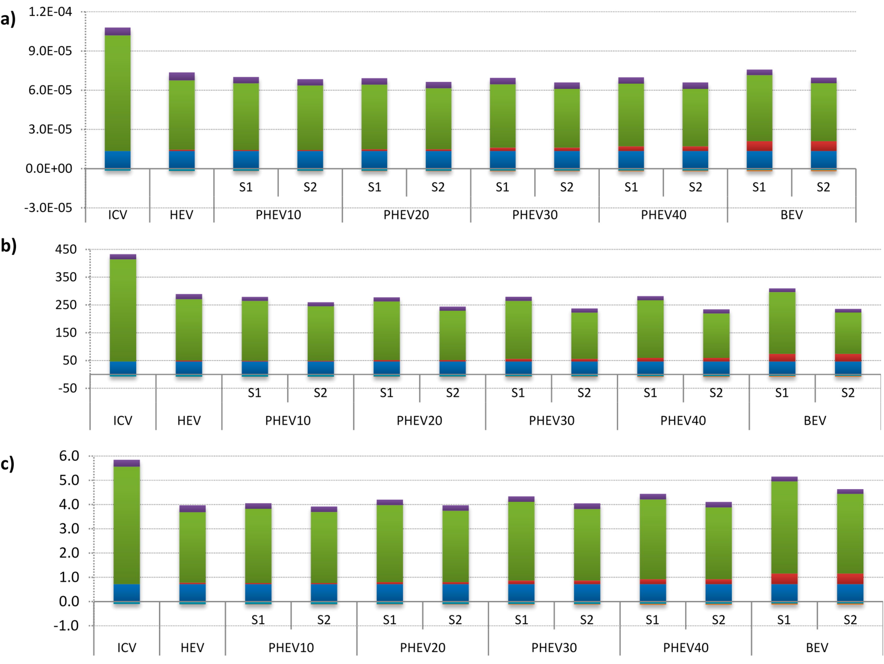
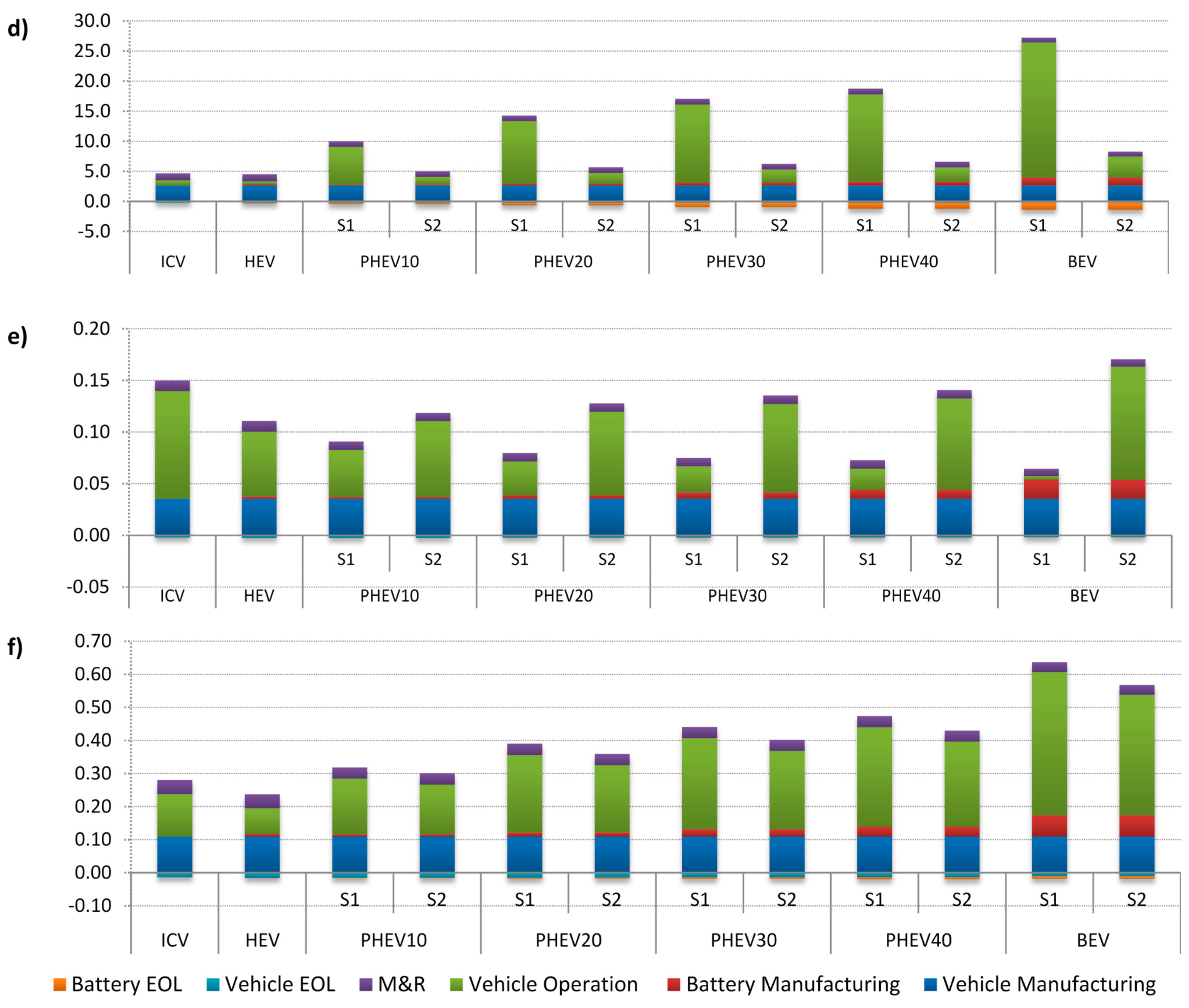
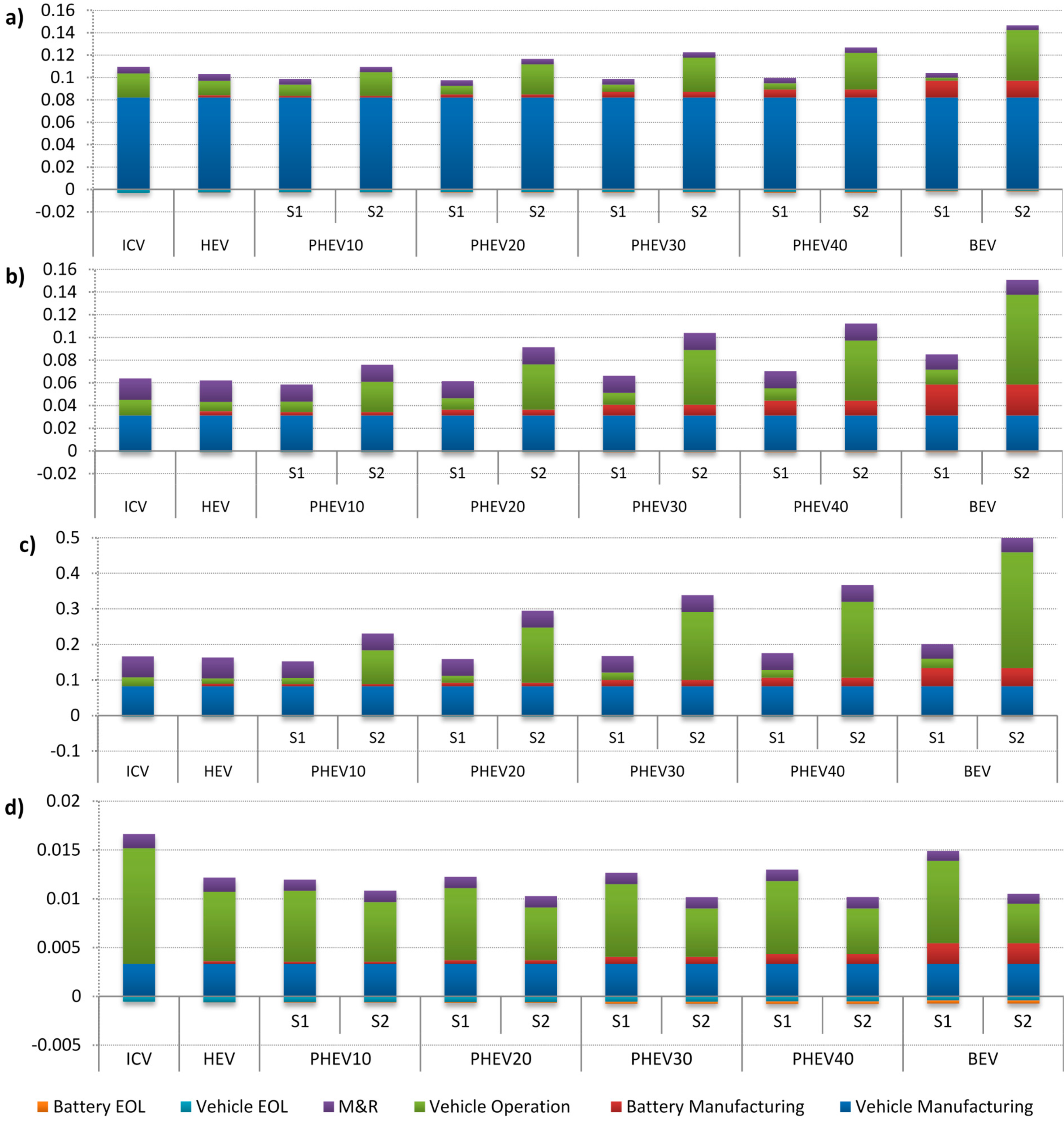
The impacts of the end-of-life phases for the vehicles and battery are calculated by determining the savings from the recycled materials from each vehicle. The material composition of each vehicle and battery are derived from the GREET vehicle cycle model using the vehicle and battery weights and the percentage of each material [83]. Once the weights of each material are found for each vehicle, these materials are assumed to be credits. [102]. Basically, the net savings from the recycling of vehicle materials is the total TBL impacts of producing each recycled material minus the TBL impacts during the recycling process of the material. While the process impacts of the recycling process of each material are available in the literature for environmental impacts, no social or economic indicators were found, and there is no sector representing the recycling process of different materials in the TBL-LCA model. Therefore, the TBL impacts from the process of recycling are neglected. In other words, the end-of-life phase includes the credits from the recycled materials provided in Table 3. Hence, in this study, the savings are less than the quantified end-of-life impacts. For more information about the quantification of end-of-life phase impacts using I-O methodology, please see the reference study [102]. Recycled materials for the batteries are copper, aluminum, and steel, and all of these materials are assumed to be 100% recycled [103,104]. Recycling rate for the vehicles are assumed to be 95% and the recycled materials are steel, aluminum, copper, plastic, rubber, and small amount of platinum [83,105]. The recycled portion of the aluminum is assumed to 90%, whereas it was assumed that 95% of all other materials were recycled [106].

3. Results

Analysis results are presented in the following subsections based on quantified economic, social, and environmental impacts attributed to each life cycle phase for each of the two analyzed scenarios. Also, the alternative vehicle technologies are compared, and their optimum allocations within the U.S. passenger vehicle stock are presented based on the proposed scenarios and quantified TBL impacts.

3.1. Environmental Impacts

Figure 2 shows the environmental impacts of the vehicles. The vehicle operation phase is the most dominant phase in all of the environmental impact categories. The ecological land footprint impacts are presented as accumulations of the five land footprint categories. The ICV has the highest impact in almost all of the environmental categories except for water withdrawals. The HEV has the second highest ecological land footprint impact, after the ICV. The ecological land footprint of BEVs is slightly higher than that of the PHEVs in both scenarios. Powering EVs and PHEVs through solar charging stations slightly reduced their ecological land footprint. In Scenario 2, the BEV has the second highest GHG emissions after the ICV due to the GHG emission intensity of electric power generation sector in the U.S. On the other hand, powering EVs via solar charging stations could reduce their GHG emissions up to 34%. This reduction potential is relatively less in PHEVs, for which it ranges between 9%–23% depending on AERs and UFs of each PHEV. Per mile energy consumption of vehicles is relatively similar to GHG impacts. It is because of the high correlation between energy consumption and GHG impacts due to the fossil fuel dependency in power generation sector. The second highest energy consumption impacts come from the BEV, and these impacts are relatively closer to each other compared to their GHG impacts. The least energy intensive vehicle option is the HEV in Scenario 1, whereas the energy performance of the PHEV10 is better than rest of the vehicles in Scenario 2. The energy consumption of BEVs and PHEVs can be reduced up to 14% by powering them with solar charging stations. There are two environmental impact categories that favor ICVs against alternative vehicle technologies, which are the water footprint and PMF. The BEV is the most water intensive vehicle and has the highest PMF in both scenarios. However, the water footprint of the BEV can be reduced by up to 85% of their operation phase water footprint by powering them with solar charging stations. While a majority of the water footprint of BEV and PHEVs is attributed to operation phase, water footprint of manufacturing and end-of-life phases are relatively much smaller. Also, hazardous waste generated through the life cycle phases of alternative vehicles are highest for ICVs in Scenario 1, with 71% generated in the operation phase of the ICV. Although the BEV generates the least hazardous waste in Scenario 1, it became the worst alternative in Scenario 2 in terms of hazardous waste due to the construction of solar charging stations and the manufacturing of the required materials which respectively account for 62% and 34% of the total hazardous waste generated to build a solar charging station.
Figure 2. Environmental impacts of alternative vehicle technologies: (a) Total ecological land footprint (gha per mile); (b) Global warming potential (gCO2-eqv. per mile); (c) Energy consumption (MJ per mile); (d) Water withdrawal (lt per mile); (e) Hazardous waste (st per mile); (f) Particulate matter formation (gPM10-eqv.).
Sustainability 06 09305 g002aSustainability 06 09305 g002b
PMF of electric vehicle options are higher than those of ICV and HEV due to air emissions from electric power generation. Although Scenario 2 reduced PMF impact of electric vehicles, the marginal reduction potential is not enough to make these options better than the conventional ICV. Construction of solar charging station and manufacturing the solar panels hindered the PMF savings of electric vehicles. However, it should be noted that the characterization factors used to calculate PMF does not include spatial variations, and therefore, their health impacts and associated economic costs differ significantly depending on the location of the emissions. These variations are included in the indicator of air emission costs. The quantified per mile emissions of criteria air pollutants are comparable with literature [82].

3.2. Economic Impacts

The economic impacts of each alternative vehicle technology are presented in Figure 3. The proposed scenarios do not affect the impacts of ICVs and HEVs and therefore, they are presented with single columns in the figure. A majority of the imports occur during the vehicle manufacturing phase, which is responsible for 57%–87% and 57%–82% of the total imports in Scenarios 1 and 2, respectively. The second most dominant phase in the terms of imports is the operation phase, the imports share of which ranges between 13% and 31% in Scenario 1 and 3%–20% in Scenario 2. On the other hand, the savings due to vehicle and battery end-of-life phases range from 1%–3%. The contribution of battery manufacturing to imports is highest for the BEV with 15% of its total life cycle imports. While the ICV yields the highest import value in Scenario 1, the BEV dominates in Scenario 2 due to high imports resulting from the purchase of solar modules to be used in solar charging stations. It is important to note that constructing solar charging station significantly increased the imports of PHEVs and EVs because of the imported solar modules to be used in constructing the solar charging stations proposed by Scenario 2. Solar modules account for 98% of the imports needed to construct a solar charging station. The rest of the materials (steel, concrete, fibreboard) accounts for a total share of only 2%. Hence, if the negative impacts associated with Scenario 2 are aimed to be minimized, the solar charging station should be manufactured domestically. It should be noted that import impacts associated with existing conditions (Scenario 1) indicate that the impacts of imports made in the operation phase of ICV are much higher than those of alternative vehicle technologies, whereas switching to renewable energy sources does not fix the issue but instead makes the situation worse.
In the business profit and GDP impact categories, alternative vehicle technologies appear to be more profitable and contribute more to the GDP than the ICV’s. Furthermore, Scenario 2 significantly increases the contribution of PHEVs and BEVs to these categories due to the construction of solar charging stations. In the business profit category, the total contributions of vehicle and battery manufacturing are more than the 50% of the total profit in Scenario 1. On the other hand, the operation phase dominates in Scenario 2 with more than 40% of the total. M&R is also an important contributor for both business profit and GDP, while end-of-life phases do not have a significant impact in either category. The BEV has the highest contribution to GDP and business profit in both scenarios. Powering BEVs with solar charging station increased the contribution of BEVs to GDP and business profit by factors of approximately 1.5 and 1.7, respectively. Hence, the positive impacts of electric vehicles on GDP and business profit can be increased significantly by constructing solar charging stations to power PHEVs and EVs.
According to location-specific costs of air emissions, operation phase is the most dominant phase whose impact ranges from 42% (BEV in S2) to 74% (ICV) of the total life cycle air emission cost. In Scenario 1, the PHEV10 has the lowest impact, whereas the ICV causes the highest economic costs due to its air emissions. Powering electric vehicles through solar charging station reduced the economic costs of air emissions of BEV by 45%. The reduction potential reduces as the AER of the PHEVs decreases. It is important to note that although solar charging stations are one of the cleanest electricity generation sources, the upstream emissions such as from manufacturing of solar panels and construction of the stations contributes to the air pollution costs significantly. Inclusion of upstream transportation services increases the external costs by as much 45% [95]. On the other hand, recycling vehicles and batteries can reduce up to 6% of the total air emission costs.
Figure 3. Economic impacts of alternative vehicle technologies: (a) Foreign Purchase ($ per mile); (b) Business Profit ($ per mile); (c) GDP ($ per mile); (d) Air emission cost ($ per mile).
Sustainability 06 09305 g003

3.3. Social Impacts

The social impacts of the each vehicle type are presented in Figure 4. In terms of the contribution to employment and income, the results are relatively close to each other in Scenario 1, whereas the contributions increase significantly if solar charging stations are built to power EVs and PHEVs. This is due primarily to the employment generated by additional construction activities, with almost 80% of the employment increase coming from the construction of new solar charging stations. On the other hand, in Scenario 1, vehicle manufacturing and M&R phases are the highest contributors to employment and income compared to other phases. In both scenarios, the BEV has the highest contribution to the employment and income impact categories.
Figure 4. Social impacts of alternative vehicle technologies: (a) Employment (Hour per mile); (b) Injuries (#worker per mile); (c) Government Tax ($ per mile); (d) Income ($ per mile); (e) Human health (DALY).
Sustainability 06 09305 g004
The contribution of the battery-manufacturing phase ranges between 3% (HEV) and 22% (BEV) in the employment and income impact categories. On the other hand, government tax draws a completely different picture due to the government incentives (federal tax credits) allocated for the purchase of PHEVs and EVs. These credits are given at the time of purchase and, are therefore associated with the automobile manufacturing phase. The taxes collected throughout the life cycle of the vehicles are highest for the ICV, and the vehicle manufacturing phase played the most crucial role in this category for every vehicle, while the M&R phase is the second highest contributor to taxes after vehicle manufacturing. On the other hand, when the operation phases of the vehicles are compared, PHEVs and the BEV generate more taxes than the ICV in both scenarios. Based on the employment, income, tax, and human health impact categories, the construction of solar charging stations is a favorable strategy to maximize these positive impacts. Allocation of income for high, medium, and low skill employees are also quantified and presented in Table 6. Electric vehicles generate slightly more income for high-skilled workers, whereas ICV generates the medium-skilled workers. On the other hand, Scenario 2 changed the skill structure of labor and increased the income allocation of medium and low skilled workers. The main reason of this structure change is the labor demand of the construction of solar charging stations and manufacturing of solar panels.
Table 6. Income allocation based on skill levels.
Income AllocationHigh-Skill CompensationMed-Skill CompensationLow-Skill Compensation
ICV 41.1%52.3%6.6%
HEV 41.4%52.1%6.6%
PHEV10S141.3%52.3%6.5%
S238.7%53.7%7.6%
PHEV20S141.4%52.2%6.4%
S237.8%54.3%7.9%
PHEV30S141.7%52.1%6.3%
S237.5%54.4%8.1%
PHEV40S141.9%51.9%6.2%
S237.5%54.5%8.1%
BEVS142.6%51.6%5.9%
S237.0%54.7%8.3%
Injuries during the operation phase of the BEV make up 70% of its life cycle impacts in Scenario 2 due to the additional construction of solar charging stations. The injuries resulting from the life cycles of BEVs are highest in both scenarios. In Scenario 1, injuries associated with automobile manufacturing contribute the most to injuries with up to 61% of the total, the second highest contributor being the M&R phase. The operation phase is responsible for the majority of the human health impact category with up to 82% of the total impacts. Adoption of electric vehicles can reduce human health impacts by up to 46% and 52% in Scenarios 1 and 2, respectively. The PHEV10 has the highest reduction potential, while this potential is up to 35% for the BEV. Scenario 2 improved the human health reduction potential of the electric vehicles up to 21%.

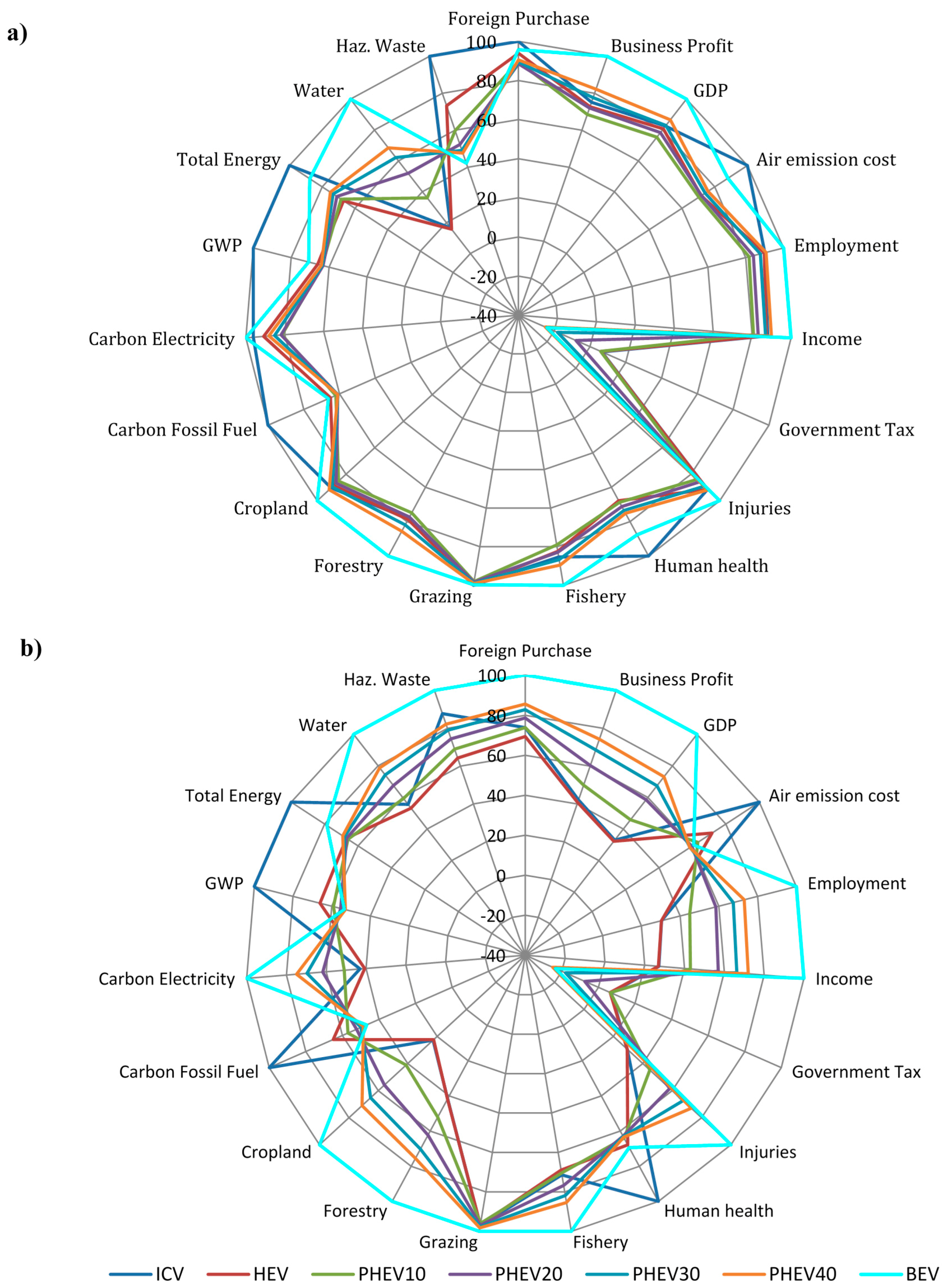
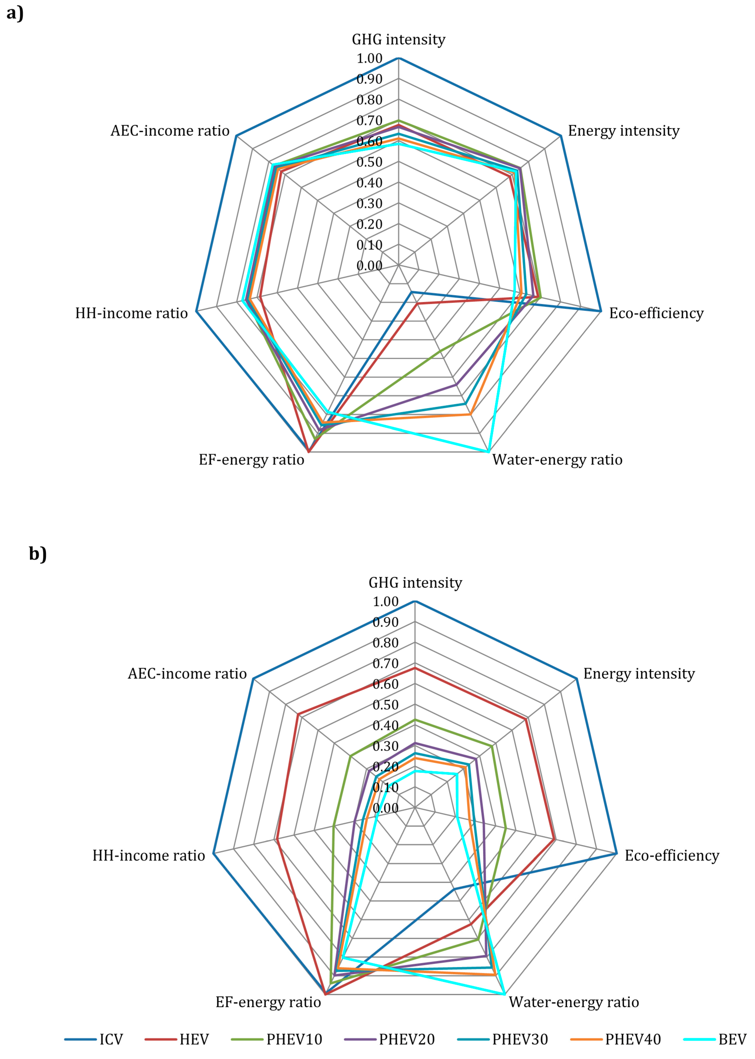
3.4. Comparison of Alternative Vehicle Technologies

In addition to the abovementioned analyses, the total life cycle TBL impacts of the vehicle alternatives are compared for Scenarios 1 and 2, and the results are shown in Figure 5.
Figure 5. Triple bottom line impact comparison of alternative vehicles: (a) Scenario 1; (b) Scenario 2.
Sustainability 06 09305 g005
Each vehicle’s pattern in the spider diagram indicates its relative contribution to or impact on each TBL category. Figure 5 highlights the anomalies where the indicators are significantly higher or lower compared to one another on the spider diagrams, depicting the relative performance of all alternative vehicle technologies in one integrated diagram. As can be seen from the figure, for most of the impact categories, the two extreme lines were represented by either the BEV or the ICV, while all other vehicle types were relatively close to each other in terms of their benchmarked impacts. However, the relative sizes of the impact differences are shown to increase considerably in Scenario 2. Although this representation allows policy makers to make a better comparison, when it comes to the selection of alternative vehicles, the selection process requires a multi objective decision making framework. Hence, the following section focuses on the optimum allocation of these vehicle technologies.
Furthermore, some sustainability metrics are provided to evaluate relative sustainability performance of alternative passenger vehicles. The quantified metrics are as follows:
  • GHG intensity: GHG emissions per $ of contribution to GDP
  • Energy intensity: Energy consumption per $ of contribution to GDP
  • Eco-efficiency: Ecological land footprint per $ of contribution to GDP
  • HH-income ratio: Human health impacts per $ of income generation
  • AEC-income ratio: Economic cost of air emission per $ of income generation
  • Water-energy ratio: Ratio of water consumption to energy consumption
  • EF-energy ratio: Ratio of ecological land footprint to energy consumption
Figure 6 shows the normalized values of these ratios for each vehicle type and for each scenario. The normalization is done by dividing each metric by the maximum value of the same metric. The normalized values are dimensionless and range from 0 to 1. These metrics indicate better sustainability performance when their values are lower.
According to sustainability metric results for Scenario 1, the sustainability performance of the BEV is superior in terms of GHG intensity, eco-efficiency, and EF-energy ratio, and the BEV is the second best option after the PHEV40 in terms of energy intensity, while the ICV had the worst performance in these same categories. The sustainability performance of the ICV is best only in terms of the water-energy ratio, where the BEV performed the worst. In Scenario 1, the HEV is found to be the best option for the metrics of HH-income and AEC-income ratios. In Scenario 2, the BEV performed the best in all categories except for the water-energy ratio, and the relative performances of all type of electric vehicles improved in comparison to the ICV. It should be noted that the environmental impacts per employment generation and contribution to business profit have very similar trends with the abovementioned sustainability metrics developed per contribution to GDP. Therefore, we did not conduct the same procedure for other positive socio-economic indicators. Additionally, the numeric values of the ratios are provided in Table 7.
Figure 6. Normalized values of sustainability metrics: (a) Scenario 1; (b) Scenario 2.
Sustainability 06 09305 g006
Table 7. Sustainability metrics for each vehicle type.
Vehicle TypesGHG Intensity (gCO2-eqv./$)Energy Intensity (MJ/$)Eco-Efficiency (gha/$)HH-Income Ratio (DALY/$)AEC-Income Ratio ($/$)Water-Energy Ratio (gal/MJ)EF-Energy Ratio (gha/MJ)
S1S2S1S2S1S2S1S2S1S2S1S2S1S2
ICV259635.06.50 × 10−47.36 × 10−60.180.201.85 × 10−5
HEV175424.04.48 × 10−45.04 × 10−60.130.291.87 × 10−5
PHEV101810110326.316.74.56 × 10−42.92 × 10−45.53 × 10−62.97 × 10−60.140.070.650.331.74 × 10−51.75 × 10⁻⁵
PHEV20172980926.213.24.32 × 10−42.21 × 10−45.55 × 10−62.20 × 10−60.140.050.910.371.65 × 10−51.68 × 10⁻⁵
PHEV30164368125.611.74.10 × 10−41.91 × 10−45.48 × 10−61.90 × 10−60.130.041.050.401.60 × 10−51.63 × 10⁻⁵
PHEV40158562025.110.93.94 × 10−41.76 × 10−45.42 × 10−61.76 × 10−60.130.041.130.421.57 × 10−51.60 × 10⁻⁵
BEV151845725.39.13.72 × 10−41.36 × 10−45.68 × 10−61.39 × 10−60.140.031.410.471.47 × 10−51.50 × 10⁻⁵

4. Conclusions and Discussions

In this article, a comprehensive macro-level sustainability assessment framework for alternative passenger vehicles in the U.S. is developed and presented. It is important to note that focusing only on the environmental aspects of this problem may misguide decision-makers and compromise important social and economic benefits while trying to reduce environmental impacts. This research also highlights the usefulness of I-O accounting for quantifying the sustainability impacts of desired systems and products. According to analysis results, the manufacturing phase is one of the most influential phases in terms of socio-economic impacts—except for human health and air emission costs—compared to other life cycle phases, whereas the operation phase is the most dominant phase in terms of environmental impacts. Scenario 2 improved the sustainability performance of the BEV and PHEVs in a majority of the indicators except in the categories of injuries, foreign purchase, and hazardous waste. The operation phase of vehicles is the most dominant phase in terms of human health and economic cost of emissions. Electric vehicles have less air pollution cost and human health impacts compared to ICVs and the emission cost and human health impact reduction potential and they can be up to 45% and 35%, respectively, if they are charged through solar charging stations. Disaggregated income allocations based on skill-levels also show the skill structure of labor demand for each vehicle type, which should be considered when developing policies since the skill-structure of the labor and market needs must match in order to implement these policies effectively [107]. Considering that globalization increased the offshoring of production, unskilled labor-intensive stages of production are likely to shift to developing countries that have more low-skilled workers, while more technologically advanced stages remain in skilled labor-abundant developed countries [108]. Although electric vehicles increase the import in Scenario 2, at the same time, they generate income for low and medium-skilled workers in the U.S.
It is also important to note that the U.S. electricity supply derives mainly from thermo-electric power plants that use large amounts of water for cooling [109,110]. The electricity sector withdraws more than 40% of all fresh water in the U.S., which is more than any other industry [111]. With the expected shift to electric vehicles, water is likely to emerge as a critical resource for transportation. Furthermore, droughts and heat waves resulting from global warming could affect cooling water resources, which could disrupt power generation [112,113]. The shift to clean energy sources could also lead to additional water use [114]. Thus, each alternative fuel option carries with it a significant water footprint, which needs to be taken into account [115]. The analysis results revealed that the water footprints of the BEV and PHEVs are much higher than those of the HEV and ICV in Scenario 1, which can be reduced significantly by powering them through solar charging stations (Scenario 2). On the other hand, the comparison of sustainability metrics showed that the relative performance of the BEV is better in a majority of the defined sustainability metrics. In Scenario 1, the BEV has the lowest GHG emissions and ecological land footprint per $ of its contribution to GDP, and has the lowest ecological footprint per unit of its energy consumption. Furthermore, Scenario 2 significantly improved the sustainability performance of all electric vehicle types, and the BEV has the lowest energy consumption, ecological land footprint, GHG emissions per $ of its contribution to GDP, human health, and economic cots of air pollutions per $ of income generation. In both of the scenarios, the only sustainability metric that does not favor the BEV is the water-energy ratio, in which case the ICV performed best.
Unfortunately, current policies seeking to promote widespread adoption of PHEVs and BEVs fail to address important social and economic factors. The planning horizon for the power generation sector is longer than that of the automotive sector, which is usually around 10–15 years. Considering that, the decisions for shifting to cleaner power generation options requires more commitment, and these decisions will play a crucial role regarding the environmental performance and widespread adoption of BEVs and PHEVs [2]. As the energy demand increases, new power infrastructure will be required in the future. The energy demand is generally met through conventional ways, mainly large power plants located far from the demand center, or through nonconventional ways, such as smaller power plants utilizing renewable energy sources. The latter is known as decentralized generation or distributed generation, which has gained interest in the power generation sector due to electricity market liberalization and environmental concerns [116]. The most popular distributed generation application is photovoltaic (PV) systems [117]. Utilization of PV systems is expected to increase since the costs of solar power technologies are declining rapidly. Furthermore, according to the EIA, on-site power generation can reduce electricity costs by 30% thanks to the savings in transmission and distribution [118]. Hence, PVs can serve as charging stations for PHEVs and BEVs and can also serve as a distributed generation source for the grid. Moreover, constructing new solar charging stations can significantly encourage the adoption of these alternative vehicle technologies and increase their market penetration.
Because quantification of sustainability impacts of alternative vehicle options is a dynamic problem, it requires multi-stage solutions and futuristic scenario evaluations. The results in this analysis are a “snapshot” in time, having been conducted based on the sector characteristics in 2002 with the latest available the TBL-LCA model and data. The updated version will be based on 2007, which still would not be able to cover the temporal aspects of the problem. The sector characteristics and their social, economic, and environmental impacts change over time However, I-O accounts are not provided annually, and there is not enough historical data to estimate the future impacts of these sectors. This is an important shortcoming of the analysis, and so high-resolution supply and use tables should be published annually and the use of I-O accounts in policy making should be supported. Furthermore, the multi-regional I-O (MRIO) models should be incorporated with the time-series I-O accounts and a time-series MRIO framework should be adopted to solve such problems. Although there are currently several initiatives aimed at compiling large-scale global MRIO data bases such as the World Input-Output Database (WIOD), the Externality Data and Input-Output Tools for Policy Analysis (EXIOPOL), the Global Trade Analysis Project (GTAP), and the EORA [119,120,121,122], their resolutions are lower and do not allow conducting product LCA due to highly aggregated sectorial data. Furthermore, there are issues with compliance of different countries’ I-O accounts due to differing numbers of sectors and a lack of standardization of sector definitions. Therefore, there is a need for improved global MRIO models that incorporate socio-economic and environmental extensions, covering the globe, and including long time series [122].
Although the current model uses high-resolution I-O tables containing 426 sectors, there are still uncertainties related to the level of aggregation in some of the sectors used to represent products such as li-ion batteries. “The primer battery manufacturing sector” includes various types of batteries besides the li-ion batteries considered in this study, and the impacts of this sector are averaged impacts of all of the output products of this sector. It is also important to note that the calculated UF’s are all national averages, and that driving patterns may vary from region to region and the quantified impacts of PHEVs might therefore be different in different regions. Driving conditions can also significantly affect the outcome of the analysis since the fuel efficiency of the vehicles is related to driving behavior and cycles [123,124].
In conclusion, a novel combined application of input–output analysis and LCSA framework is presented as a sustainability assessment framework to evaluate alternative passenger vehicles in the U.S. With further developments in I-O research, better models that encompass temporal and spatial variations can be introduced, and thus better frameworks can be presented in the future. In this regard, the inclusion of a system dynamic perspective can lead to a better understanding of the system behavior and improve the effectiveness of future policies [125]. Understanding system behavior is essential to reveal the dynamic relationship between the social, economic, and environmental impacts associated with adoption of alternative vehicle options, because the transportation sector and the adoption of alternative vehicles each involve a series of interconnected causal relationships that will need to be analyzed from a systems thinking perspective.

Acknowledgments

This material is based upon work supported in part by the Electric Vehicle Transportation Center funded by the U.S. Department of Transportation University Transportation Centers Program.

Authors Contributions

Nuri C. Onat carried out the analyses including work related to LCSA, life cycle inventory, data collection and processing and wrote majority of the manuscript. Murat Kucukvar contributed the TBL-LCA methodology and literature review parts. Omer Tatari supervised the research and contributed to the framework of the sustainability metrics. All of the authors contributed to preparing and approving the manuscript.

Conflicts of Interest

The authors declare no conflict of interest.

References

  1. Onat, N.C.; Kucukvar, M.; Tatari, O. Conventional, Hybrid, Plug-in Hybrid or Electric Vehicles? State-based Comparative Carbon and Energy Footprint Analysis in the United States. Appl. Energy 2014, in press. [Google Scholar]
  2. Samaras, C.; Meisterling, K. Life Cycle Assessment of Greenhouse Gas Emissions from Plug-in Hybrid Vehicles: Implications for Policy. Environ. Sci. Technol. 2008, 42, 3170–3176. [Google Scholar] [CrossRef] [PubMed]
  3. Kucukvar, M.; Noori, M.; Egilmez, G.; Tatari, O. Stochastic decision modeling for sustainable pavement designs. Int. J. Life Cycle Assess. 2014, 19, 1185–1199. [Google Scholar] [CrossRef]
  4. Oak Ridge National Lab. Transportation Energy Data book. Available online: http://cta.ornl.gov/data/chapter8.shtml (accessed on 8 July 2013).
  5. Melaina, M.; Bremson, J. Refueling availability for alternative fuel vehicle markets: Sufficient urban station coverage. Energy Policy 2008, 36, 3233–3241. [Google Scholar] [CrossRef]
  6. DOT U.S. Department of Transportation Proposes New Minimum Sound Requirements for Hybrid and Electric Vehicles. Available online: http://www.dot.gov/briefing-room/us-department-transportation-proposes-new-minimum-sound-requirements-hybrid-and (accessed on 3 December 2014).
  7. Executive Office of the President. President Obama’s Climate Action Plan; Executive Office of the President: Washington, DC, USA, 2013; p. 9. [Google Scholar]
  8. Intergovernmental Panel on Climate Change (IPCC). Mitigation of Climate Change: Contribution of Working Group III to the Fourth Assessment Report of the Intergovernmental Panel on Climate Change; Cambridge University Press: Cambridge, UK, 2007; p. 851. [Google Scholar]
  9. World Business Council for Sustainable Development (WBCSD). Mobility 2030: Meeting the Challenges to Sustainability; WBCSD: Geneva, Switzerland, 2004. [Google Scholar]
  10. Department of Energy (DOE). One Million Electric Vehicles By 2015; DOE: Washington, DC, USA, 2011. [Google Scholar]
  11. Department of Energy (DOE). The EV Everywhere Grand Challenge; DOE: Washington, DC, USA, 2013. [Google Scholar]
  12. Litman, T.A. Sustainable Transportation Indicators: A Recommended Research Program For Developing Sustainable Transportation Indicators and Data. In Proceedings of the Transportation Research Board 88th Annual Meeting, Washington, DC, USA, 11–15 January 2009.
  13. Hawkins, T.R.; Gausen, O.M.; Strømman, A.H. Environmental impacts of hybrid and electric vehicles—A review. Int. J. Life Cycle Assess. 2012, 17, 997–1014. [Google Scholar] [CrossRef]
  14. Shepherd, S.P. A review of system dynamics models applied in transportation. Trans. B Trans. Dyn. 2014, 2, 83–105. [Google Scholar]
  15. Litman, T.; Burwell, D. Issues in sustainable transportation. Int. J. Glob. Environ. Issues 2006, 6, 331–347. [Google Scholar] [CrossRef]
  16. Forkenbrock, D.; Benshoff, S.; Weisbrod, G. Assessing the Social and Economic Effects of Transportation Projects; Transportation Research Board: Iowa City, IA, USA, 2001. [Google Scholar]
  17. Offer, G.J.; Howey, D.; Contestabile, M.; Clague, R.; Brandon, N.P. Comparative analysis of battery electric, hydrogen fuel cell and hybrid vehicles in a future sustainable road transport system. Energy Policy 2010, 38, 24–29. [Google Scholar] [CrossRef] [Green Version]
  18. Stone, S.; Strutt, A.; Hertel, T. Socio-Economic Impact of Regional Transport Infrastructure in the Greater Mekong Subregion. In Infrastructure for Asian Connectivity; Edward Elgar Publishing: Cheltenham, UK, 2012. [Google Scholar]
  19. The World Bank. Social Analysis in Transportation Projects: Guidelines for Incorporating Social Dimensions into Bank-Supported Projects; The World Bank: Washington, DC, USA, 2006. [Google Scholar]
  20. Dobranskyte-Niskota, A.; Perujo, A.; Pregl, M. Indicators to Assess Sustainability of Transport Activities; European Comission, Joint Research Centre: Ispra, Italy, 2007. [Google Scholar]
  21. Rebitzer, G.; Ekvall, T.; Frischknecht, R.; Hunkeler, D.; Norris, G.; Rydberg, T.; Schmidt, W.-P.; Suh, S.; Weidema, B.P.; Pennington, D.W. Life cycle assessment part 1: Framework, goal and scope definition, inventory analysis, and applications. Environ. Int. 2004, 30, 701–720. [Google Scholar] [CrossRef] [PubMed]
  22. Finnveden, G.; Hauschild, M.Z.; Ekvall, T.; Guinée, J.; Heijungs, R.; Hellweg, S.; Koehler, A.; Pennington, D.; Suh, S. Recent developments in Life Cycle Assessment. J. Environ. Manag. 2009, 91, 1–21. [Google Scholar] [CrossRef]
  23. Suh, S.; Lenzen, M.; Treloar, G.J.; Hondo, H.; Horvath, A.; Huppes, G.; Jolliet, O.; Klann, U.; Krewitt, W.; Moriguchi, Y.; et al. System Boundary Selection in Life-Cycle Inventories Using Hybrid Approaches. Environ. Sci. Technol. 2004, 38, 657–664. [Google Scholar] [CrossRef] [PubMed]
  24. Deng, L.; Babbitt, C.W.; Williams, E.D. Economic-balance hybrid LCA extended with uncertainty analysis: Case study of a laptop computer. J. Clean. Prod. 2011, 19, 1198–1206. [Google Scholar] [CrossRef]
  25. Norgate, T.E.; Jahanshahi, S.; Rankin, W.J. Assessing the environmental impact of metal production processes. J. Clean. Prod. 2007, 15, 838–848. [Google Scholar] [CrossRef]
  26. De Benedetto, L.; Klemeš, J. The Environmental Performance Strategy Map: An integrated LCA approach to support the strategic decision-making process. J. Clean. Prod. 2009, 17, 900–906. [Google Scholar] [CrossRef]
  27. Onat, N.C.; Kucukvar, M.; Tatari, O. Scope-based carbon footprint analysis of U.S. residential and commercial buildings: An input–output hybrid life cycle assessment approach. Build. Environ. 2014, 72, 53–62. [Google Scholar] [CrossRef]
  28. Hendrickson, C.; Lave, L.B.; Matthews, H.S. Environmental Life Cycle Assessment of Goods and Services: An Input-Output Approach; Routledge: London, UK, 2006. [Google Scholar]
  29. Egilmez, G.; Kucukvar, M.; Tatari, O. Sustainability assessment of U.S. manufacturing sectors: An economic input output-based frontier approach. J. Clean. Prod. 2013, 53, 91–102. [Google Scholar] [CrossRef]
  30. Kucukvar, M.; Tatari, O. Towards a triple bottom-line sustainability assessment of the U.S. construction industry. Int. J. Life Cycle Assess. 2013, 18, 958–972. [Google Scholar] [CrossRef]
  31. Lenzen, M. Errors in Conventional and Input-Output based Life-Cycle Inventories. J. Ind. Ecol. 2000, 4, 127–148. [Google Scholar] [CrossRef]
  32. Matthews, H.S.; Hendrickson, C.T.; Weber, C.L. The Importance of Carbon Footprint Estimation Boundaries. Environ. Sci. Technol. 2008, 42, 5839–5842. [Google Scholar] [CrossRef] [PubMed]
  33. Hertwich, E.G.; Peters, G.P. Carbon Footprint of Nations: A Global, Trade-Linked Analysis. Environ. Sci. Technol. 2009, 43, 6414–6420. [Google Scholar] [CrossRef] [PubMed]
  34. Onat, N.C.; Kucukvar, M.; Tatari, O. Integrating triple bottom line input–output analysis into life cycle sustainability assessment framework: The case for US buildings. Int. J. Life Cycle Assess. 2014, 19, 1488–1505. [Google Scholar] [CrossRef]
  35. Kucukvar, M.; Egilmez, G.; Tatari, O. Sustainability assessment of U.S. final consumption and investments: Triple-bottom-line input–output analysis. J. Clean. Prod. 2014, 81, 234–243. [Google Scholar] [CrossRef]
  36. Sala, S.; Farioli, F.; Zamagni, A. Life cycle sustainability assessment in the context of sustainability science progress (part 2). Int. J. Life Cycle Assess. 2012, 18, 1686–1697. [Google Scholar] [CrossRef]
  37. Zamagni, A. Life cycle sustainability assessment. Int. J. Life Cycle Assess. 2012, 17, 373–376. [Google Scholar] [CrossRef]
  38. Ciroth, A.; Finkbeier, M.; Hildenbrand, J.; Klöpffer, W.; UGent, B.M.; Prakash, S.; Sonnemann, G.; Traverso, M.; Ugaya, C.M.L.; Valdivia, S.; et al. Towards a Live Cycle Sustainability Assessment: Making Informed Choices on Products; United Nations Environment Programme (UNEP): Nairobi, Kenya, 2011. [Google Scholar]
  39. Guinée, J.B.; Heijungs, R.; Huppes, G.; Zamagni, A.; Masoni, P.; Buonamici, R.; Ekvall, T.; Rydberg, T. Life cycle assessment: Past, present, and future. Environ. Sci. Technol. 2011, 45, 90–96. [Google Scholar] [CrossRef] [PubMed]
  40. Valdivia, S.; Ugaya, C.; Sonnemann, G.; Hildenbrand, J. Towards a Life Cycle Sustainability Assessment-Making Informed Choices on Products. UNEP/SETAC Life Cycle Initiative. Available online: http://www.unep.org/publications/contents/pub_details_search.asp?ID=6236 (accessed on 12 December 2014).
  41. United Nations Environment Programme (UNEP). Towards a Life Cycle Sustainability Assessment: Making Informed Choices on Products; UNEP: Nairobi, Kenya, 2011. [Google Scholar]
  42. Kloepffer, W. Life cycle sustainability assessment of products. Int. J. Life Cycle Assess. 2008, 13, 89–95. [Google Scholar] [CrossRef]
  43. Finkbeiner, M.; Schau, E.M.; Lehmann, A.; Traverso, M. Towards Life Cycle Sustainability Assessment. Sustainability 2010, 2, 3309–3322. [Google Scholar] [CrossRef]
  44. Valdivia, S.; Ugaya, C.M.L.; Hildenbrand, J.; Traverso, M.; Mazijn, B.; Sonnemann, G. A UNEP/SETAC approach towards a life cycle sustainability assessment—Our contribution to Rio+20. Int. J. Life Cycle Assess. 2012, 18, 1673–1685. [Google Scholar] [CrossRef]
  45. Hu, M.; Kleijn, R.; Bozhilova-Kisheva, K.P.; di Maio, F. An approach to LCSA: The case of concrete recycling. Int. J. Life Cycle Assess. 2013, 18, 1793–1803. [Google Scholar] [CrossRef]
  46. Traverso, M.; Asdrubali, F.; Francia, A.; Finkbeiner, M. Towards life cycle sustainability assessment: An implementation to photovoltaic modules. Int. J. Life Cycle Assess. 2012, 17, 1068–1079. [Google Scholar] [CrossRef]
  47. Wood, R.; Hertwich, E.G. Economic modelling and indicators in life cycle sustainability assessment. Int. J. Life Cycle Assess. 2012, 18, 1710–1721. [Google Scholar] [CrossRef]
  48. Nanaki, E.A.; Koroneos, C.J. Comparative economic and environmental analysis of conventional, hybrid and electric vehicles–the case study of Greece. J. Clean. Prod. 2013, 53, 261–266. [Google Scholar] [CrossRef]
  49. Strecker, B.; Hausmann, A.; Depcik, C. Well to wheels energy and emissions analysis of a recycled 1974 VW Super Beetle converted into a plug-in series hybrid electric vehicle. J. Clean. Prod. 2014, 68, 93–103. [Google Scholar]
  50. Faria, R.; Moura, P.; Delgado, J.; de Almeida, A.T. A sustainability assessment of electric vehicles as a personal mobility system. Energy Convers. Manag. 2012, 61, 19–30. [Google Scholar] [CrossRef]
  51. Nordelöf, A.; Messagie, M.; Tillman, A.-M.; Ljunggren Söderman, M.; van Mierlo, J. Environmental impacts of hybrid, plug-in hybrid, and battery electric vehicles—What can we learn from life cycle assessment? Int. J. Life Cycle Assess. 2014, 19, 1866–1890. [Google Scholar] [CrossRef]
  52. Markel, T. Plug-In HEV Vehicle Design Options and Expectations. In Proceedings of the ZEV Technology Symposium California Air Resources Board, Sacramento, CA, USA, 27 September 2006.
  53. Leontief, W. Environmental Repercussions and the Economic Structure: An Input-Output Approach. Rev. Econ. Stat. 1970, 52, 262–271. [Google Scholar] [CrossRef]
  54. Murray, J.; Wood, R. The Sustainability Practitioner’s Guide to Input-Output Analysis; Common Ground Publishing: Champaign, IL, USA, 2010. [Google Scholar]
  55. Tukker, A.; Poliakov, E.; Heijungs, R.; Hawkins, T.; Neuwahl, F.; Rueda-Cantuche, J.M.; Giljum, S.; Moll, S.; Oosterhaven, J.; Bouwmeester, M. Towards a global multi-regional environmentally extended input–output database. Ecol. Econ. 2009, 68, 1928–1937. [Google Scholar] [CrossRef]
  56. BEA Benchmark input-output data. Available online: http://www.bea.gov/iTable/iTable.cfm?ReqID=5&step=1#reqid=5&step=100&isuri=1&406=3&403=2&404=7 (accessed on 19 May 2014).
  57. BEA 2002 Benchmark Input-Output-Item Output Detail. Available online: http://www.bea.gov/industry/xls/2002DetailedItemOutput.xls&ei=nxqHUbT-EIie8QSn74HgCA&usg=AFQjCNEOABYqv8MJKxkgHKmjU54cTqMCxQ&sig2=4eDqdCLk_kuEpu6PgEu9Dg (accessed on 19 May 2013).
  58. Carnegie Mellon University Green Design Institute Economic Input-Output Life Cycle Assessment (EIO-LCA). Available online: http://www.eiolca.net/index.html (accessed on 9 March 2014).
  59. OSU—The Ohio State University Eco-LCA software, ecologically based life cycle assessment. Available online: http://resilience.eng.ohio-state.edu/eco-lca/index.htm (accessed on 9 March 2014).
  60. Foran, B.; Lenzen, M.; Dey, C.; Bilek, M. Integrating sustainable chain management with triple bottom line accounting. Ecol. Econ. 2005, 52, 143–157. [Google Scholar] [CrossRef]
  61. Wiedmann, T.; Lenzen, M. Unravelling the Impacts of Supply Chains—A New Triple-Bottom-Line Accounting Approach and Software Tool. Manag. Account. Clean. Prod. 2009, 24, 65–90. [Google Scholar]
  62. Eurostat. Eurostat Manual of Supply, Use and Input–Output Tables; Eurostat: Luxembourg, 2008. [Google Scholar]
  63. United Nations. UN (1999) Studies in Methods: Handbook of National Accounting; United Nations: New York, NY, USA, 1999. [Google Scholar]
  64. Miller, R.E.; Blair, P.D. Input–Output Analysis: Foundations and Extensions, 2nd ed.; Cambridge University Press: Cambridge, UK, 2009. [Google Scholar]
  65. U.S. Bureau of Labor Statistics. Industry Injury and Illness Data; U.S. Bureau of Labor Statistics: Washington, DC, USA, 2002; pp. 2–28. [Google Scholar]
  66. Global Footprint Network (GFN) National footprint accounts: Ecological footprint and bio-capacity. Available online: http://www.footprintnetwork.org/en/index.php/GFN/page/footprint_for_nations (accessed on 21 June 2014).
  67. Wiedmann, T.O.; Lenzen, M.; Barrett, J.R. Companies on the Scale: Comparing and benchmarking the sustainability performance of businesses. J. Ind. Ecol. 2009, 13, 361–383. [Google Scholar] [CrossRef]
  68. Timmer, M.; Erumban, A.; Gouma, R. The world input-output database (WIOD): Contents, sources and methods. Available online: http://www.wiod.org/publications/papers/wiod10.pdf (accessed on 26 November 2014).
  69. Erumban, A.; Gouma, R.; de Vries, G.; de Vries, K.; Timmer, M. WIOD Socio-Economic Accounts (SEA): Sources and Methods. Available online: http://www.wiod.org/publications/source_docs/SEA_Sources.pdf (accessed on 20 November 2014).
  70. Stern, J.; Lewis, J. Employment Patterns and Income Growth: An Application of Input-Output Analysis; The World Bank: Washington, DC, USA, 1980. [Google Scholar]
  71. World Health Organization Health statistics and information systems, Metrics: Disability-Adjusted Life Year (DALY). Available online: http://www.who.int/healthinfo/global_burden_disease/metrics_daly/en/ (accessed on 26 November 2014).
  72. ReCiPE ReCiPe LCIA Methodology. Available online: http://www.lcia-recipe.net/project-definition (accessed on 26 November 2014).
  73. De Schryver, A.M.; Brakkee, K.W.; Goedkoop, M.J.; Huijbregts, M.A.J. Characterization Factors for Global Warming in Life Cycle Assessment Based on Damages to Humans and Ecosystems. Environ. Sci. Technol. 2009, 43, 1689–1695. [Google Scholar] [CrossRef] [PubMed]
  74. De Schryver, A.M.; van Zelm, R.; Humbert, S.; Pfister, S.; McKone, T.E.; Huijbregts, M.A.J. Value Choices in Life Cycle Impact Assessment of Stressors Causing Human Health Damage. J. Ind. Ecol. 2011, 15, 796–815. [Google Scholar] [CrossRef] [Green Version]
  75. De Schryver, A.; van Zelm, R.; Humbert, S.; McKone, T.E.; Huijbregts, M.A.J. Value choices in human health endpoint modelling. Available online: http://www.lcacenter.org/LCA9/presentations/77.pdf (accessed on 26 November 2014).
  76. Tukker, A. Risk Analysis, Life Cycle Assessment-The Common Challenge of Dealing with the Precautionary Frame (Based on the Toxicity Controversy in Sweden and the Netherlands). Risk Anal. 2002, 22, 821–832. [Google Scholar] [CrossRef] [PubMed]
  77. Michalek, J.J.; Chester, M.; Jaramillo, P.; Samaras, C.; Shiau, C.-S.N.; Lave, L.B. Valuation of plug-in vehicle life-cycle air emissions and oil displacement benefits. Proc. Natl. Acad. Sci. USA 2011, 108, 16554–16558. [Google Scholar] [CrossRef] [PubMed]
  78. Kopp, R.E.; Mignone, B.K. The U.S. Government’s Social Cost of Carbon Estimates after Their First Two Years: Pathways for Improvement. Econ. Open-Access Open-Assess. E-J. 2012, 6, 1–41. [Google Scholar]
  79. US Interagency Working Group on Social Cost of Carbon. Technical Support Document: Social Cost of Carbon for Regulatory Impact Analysis Under Executive Order 12866; US Interagency Working Group on Social Cost of Carbon: Washington, DC, USA, 2010. [Google Scholar]
  80. Tatari, O.; Kucukvar, M. Sustainability Assessment of U.S. Construction Sectors: Ecosystems Perspective. J. Constr. Eng. Manag. 2012, 138, 918–922. [Google Scholar] [CrossRef]
  81. Burnham, A.; Wang, M.; Wu, Y. Development and Applications of GREET 2.7—The Transportation Vehicle-Cycle Model; U.S. Department of Energy: Oak Ridge, TN, USA, 2009. [Google Scholar]
  82. Marshall, B.M.; Kelly, J.C.; Lee, T.-K.; Keoleian, G.A.; Filipi, Z. Environmental assessment of plug-in hybrid electric vehicles using naturalistic drive cycles and vehicle travel patterns: A Michigan case study. Energy Policy 2013, 58, 358–370. [Google Scholar] [CrossRef]
  83. Argonne Transportation Technology R&D Center GREET Vehicle cycle model. Available online: https://greet.es.anl.gov/greet_2_series (accessed on 7 August 2014).
  84. Autonomie Argonne Transportation Technology R&D Center. Available online: http://www.transportation.anl.gov/modeling_simulation/PSAT/autonomie.html (accessed on 8 September 2014).
  85. Elgowainy, A.; Burnham, A. Well-to-wheels energy use and greenhouse gas emissions of plug-in hybrid electric vehicles. SAE Int. J. Fuels Lubr. 2009, 2, 627–644. [Google Scholar]
  86. Argonne Transportation Technology R&D Center. Costs of Lithium-Ion Batteries for Vehicles; Argonne Transportation Technology R&D Center: Argonne, IL, USA, 2000. [Google Scholar]
  87. U.S. DEO Federal Tax Credits for Plug-in Hybrids. Available online: http://www.fueleconomy.gov/feg/taxphevb.shtml (accessed on 7 December 2014).
  88. Toyota 2014 Toyota Corolla Specifications. Available online: http://www.toyota.com/corolla/#!/Welcome (accessed on 9 January 2014).
  89. Toyota 2014 Toyota Prius-HEV Specifications. Available online: http://www.toyota.com/prius/features.html#!/weights_capacities/1223/1225/1227/1229 (accessed on 1 September 2014).
  90. Nissan 2014 Nissan Leaf Specifications. Available online: http://www.nissanusa.com/electric-cars/leaf/versions-specs/ (accessed on 1 September 2014).
  91. Toyota 2014 Toyota Prius-PHEV Specifications. Available online: http://www.toyota.com/prius-plug-in/features.html#!/mechanical/1235/1237 (accessed on 2 February 2014).
  92. Chevrolet 2014 Chevrolet Volt Specifications. Available online: http://www.chevrolet.com/volt-electric-car/specs/dimensions.html (accessed on 1 September 2014).
  93. EPA Gasoline Emission Factor-Calculations and References. Available online: http://www.epa.gov/cleanenergy/energy-resources/refs.html (accessed on 10 November 2013).
  94. U.S. Environmental Protection Agency Office of Transportation and Air Quality. Fuel Economy Labeling of Motor Vehicles: Revisions to Improve Calculation of Fuel Economy Estimates; U.S. Environmental Protection Agency Office of Transportation and Air Quality: Washington, DC, USA, 2006. [Google Scholar]
  95. Matthews, H.S.; Hendrickson, C.; Horvath, A. External Costs of Air Emissions from Transportation. J. Infrastruct. Syst. 2001, 7, 13–17. [Google Scholar] [CrossRef]
  96. The U.S. Department of Transportation. National Household Survey-Summary of Household Travel Trends; The U.S. Department of Transportation: Washington, DC, USA, 2009. [Google Scholar]
  97. National Household Travel Survey Online Analysis Tools—Table Designer. Available online: http://nhts.ornl.gov/tools.shtml (accessed on 3 July 2014).
  98. Engholm, A.; Johansson, G.; Persson, A.Å. Life Cycle Assessment: Of Solelia Greentech’s Photovoltaic BasedCharging Station for Electric Vehicles. Available online: http://www.diva-portal.org/smash/get/diva2:626019/FULLTEXT01.pdf (accessed on 9 December 2014).
  99. Transportation Energy Data book Transportation and the Economy-Car Operating Cost per Mile, 1985–2012. Available online: http://cta.ornl.gov/data/chapter10.shtml (accessed on 19 January 2014).
  100. Faria, R.; Marques, P.; Moura, P.; Freire, F.; Delgado, J.; de Almeida, A.T. Impact of the electricity mix and use profile in the life-cycle assessment of electric vehicles. Renew. Sustain. Energy Rev. 2013, 24, 271–287. [Google Scholar] [CrossRef]
  101. Delucchi, M.A.; Lipman, T.E. An analysis of the retail and lifecycle cost of battery-powered electric vehicles. Transp. Res. Part D Transp. Environ. 2001, 6, 371–404. [Google Scholar] [CrossRef]
  102. Joshi, S. Product Environmental Life-Cycle Assessment Using Input-Output Techniques. J. Ind. Ecol. 1999, 3, 95–120. [Google Scholar] [CrossRef]
  103. Gaines, L.; Nelson, P. Lithium-ion Batteries: Examining Material Demand and Recycling Issues; Argonne National Laboratory: Argonne, IL, USA, 2010. [Google Scholar]
  104. Gaines, L.; Sullivan, J.; Burnham, A.; Belharouak, I. Life-Cycle Analysis for Lithium-Ion Battery Production and Recycling. Trans. Res. Record J. Trans. Res. Board 2010. [Google Scholar] [CrossRef]
  105. Jody, B.J.; Duranceau, C.M.; Daniels, E.J.; Pomykala, A.J. End-of-Life Vehicle Recycling: State of the Art of Resource Recovery from Shredder Residue. Available online: http://www.osti.gov/scitech/biblio/925337 (accessed on 12 December 2014).
  106. EPA Wastes-Resource Conservation-Common Wastes & Materials. Available online: http://www.epa.gov/epawaste/conserve/materials/auto.htm (accessed on 8 September 2014).
  107. World Economic Forum Global Agenda Council on Employment. Matching Skills and Labour Market Needs Building Social Partnerships for Better Skills and Better Jobs. Available online: http://www.weforum.org/reports/matching-skills-and-labour-market-needs-building-social-partnerships-better-skills-and-bette (accessed on 12 December 2014).
  108. Foster-McGregor, N.; Stehrer, R.; de Vries, G.J. Offshoring and the skill structure of labour demand. Rev. World Econ. 2013, 149, 631–662. [Google Scholar] [CrossRef]
  109. Energy Information Administration (EIA). ternational Energy Outlook 2010; EIA: Washington, DC, USA, 2010. [Google Scholar]
  110. Cameron, C.; Yelverton, W.; Dodder, R.; West, J. Strategic responses to CO2 emission reduction targets drive shift in US electric sector water use. Energy Strateg. Rev. 2014, 4, 16–27. [Google Scholar] [CrossRef]
  111. Kenny, J.F.; Barber, N.L.; Hutson, S.S.; Linsey, K.S.; Lovelace, J.K.; Maupin, M.A. Estimated Use of Water in the United States in 2005; U.S. Geological Survey Circular: Reston, VA, USA, 2009. [Google Scholar]
  112. Kimmell, T.; Veil, J. Impact of Drought on US Steam Electric Power Plant Cooling Water Intakes and Related Water Resource Management Issues; Argonne National Laboratory Environmental Science Division: Argonne, IL, USA, 2009. [Google Scholar]
  113. Zamuda, C.; Mignone, B.; Bilello, D.; Hallett, K. US Energy Sector Vulnerabilities to Climate Change and Extreme Weather; The U.S. Department of Energy: Washington, DC, USA, 2013. [Google Scholar]
  114. Harto, C.; Meyers, R.; Williams, E. Life cycle water use of low-carbon transport fuels. Energy Policy 2010, 9, 4933–4944. [Google Scholar] [CrossRef]
  115. King, C.; Webber, M. Water intensity of transportation. Environ. Sci. Technol. 2008, 42, 7866–7872. [Google Scholar] [CrossRef] [PubMed]
  116. Pepermans, G.; Driesen, J.; Haeseldonckx, D.; Belmans, R.; D’haeseleer, W. Distributed generation: Definition, benefits and issues. Energy Policy 2005, 33, 787–798. [Google Scholar] [CrossRef]
  117. Li, X.; Lopes, L.A.C.; Williamson, S.S. On the suitability of plug-in hybrid electric vehicle (PHEV) charging infrastructures based on wind and solar energy. In Proceedings of the 2009 IEEE Power & Energy Society General Meeting, Calgary, AB, Canada, 26–30 July 2009; pp. 1–8.
  118. The U.S. Energy Information Administration (EIA). Annual Energy Outlook with Projections to 2040; EIA: Washington, DC, USA, 2013. [Google Scholar]
  119. Andrew, R.M.; Peters, G.P. A Multi-Region Input–Output Table Based On the Global Trade Analysis Project Database (GTAP-MRIO). Econ. Syst. Res. 2013, 25, 99–121. [Google Scholar] [CrossRef]
  120. Dietzenbacher, E.; Los, B.; Stehrer, R.; Timmer, M.; de Vries, G. The Construction of World Input–Output Tables in the WIOD Project. Econ. Syst. Res. 2013, 25, 71–98. [Google Scholar] [CrossRef]
  121. Lenzen, M.; Moran, D.; Kanemoto, K.; Geschke, A. Building EORA: A Global Multi-Region Input–Output Database at High Country And Sector Resolution. Econ. Syst. Res. 2013, 25, 20–49. [Google Scholar] [CrossRef]
  122. Tukker, A.; Dietzenbacher, E. Global Multiregional Input–Output Frameworks: An Introduction and Outlook. Econ. Syst. Res. 2013, 25, 1–19. [Google Scholar] [CrossRef]
  123. Raykin, L.; MacLean, H.L.; Roorda, M.J. Implications of driving patterns on well-to-wheel performance of plug-in hybrid electric vehicles. Environ. Sci. Technol. 2012, 46, 6363–6370. [Google Scholar] [CrossRef] [PubMed]
  124. Karabasoglu, O.; Michalek, J. Influence of driving patterns on life cycle cost and emissions of hybrid and plug-in electric vehicle powertrains. Energy Policy 2013, 60, 445–461. [Google Scholar] [CrossRef]
  125. Onat, N.C.; Egilmez, G.; Tatari, O. Towards greening the U.S. residential building stock: A system dynamics approach. Build. Environ. 2014, 78, 68–80. [Google Scholar] [CrossRef]

