Article

Modeling a Sustainable Salt Tolerant Grass-Livestock Production System under Saline Conditions in the Western San Joaquin Valley of California

1
Department of Environmental Sciences and Natural Resources, University of Chile, Santa Rosa 11315, La Pintana, Santiago, Chile
2
USDA-ARS United States Salinity Laboratory, 450 West Big Springs Road, Riverside, CA 92507, USA
3
Department of Environmental Sciences, University of California at Riverside, 900 University Ave., Riverside, CA 92521, USA
4
Department of Animal Science, University of California at Davis, One Shields Ave., Davis, CA 95616, USA
5
Department of Plant Sciences, University of California at Davis, One Shields Ave., Davis, CA 95616, USA
*
Author to whom correspondence should be addressed.
Sustainability 2013, 5(9), 3839-3857; https://doi.org/10.3390/su5093839
Submission received: 23 June 2013 / Revised: 3 September 2013 / Accepted: 5 September 2013 / Published: 10 September 2013

Abstract

:
Salinity and trace mineral accumulation threaten the sustainability of crop production in many semi-arid parts of the world, including California’s western San Joaquin Valley (WSJV). We used data from a multi-year field-scale trial in Kings County and related container trials to simulate a forage-grazing system under saline conditions. The model uses rainfall and irrigation water amounts, irrigation water quality, soil, plant, and atmospheric variables to predict Bermuda grass (Cynodon dactylon (L.) Pers.) growth, quality, and use by cattle. Simulations based on field measurements and a related container study indicate that although soil chemical composition is affected by irrigation water quality, irrigation timing and frequency can be used to mitigate salt and trace mineral accumulation. Bermuda grass yields of up to 12 Mg dry matter (DM)·ha−1 were observed at the field site and predicted by the model. Forage yield and quality supports un-supplemented cattle stocking rates of 1.0 to 1.2 animal units (AU)·ha−1. However, a balance must be achieved between stocking rate, desired average daily gain, accumulation of salts in the soil profile, and potential pollution of ground water from drainage and leaching. Using available weather data, crop-specific parameter values and field scale measurements of soil salinity and nitrogen levels, the model can be used by farmers growing forages on saline soils elsewhere, to sustain forage and livestock production under similarly marginal conditions.

1. Introduction

The semi-arid western San Joaquin Valley (WSJV) has large areas with shallow, saline water tables that limit crop choice, reduce productivity, and has led to land idling or abandonment. The amount of land affected in this way is reported to vary up to 200,000 ha, depending on rainfall and irrigation water delivered to the region [1,2]. To farm this land sustainably, subsurface drainage is required. But agricultural drainage water in this region often contains trace minerals such as selenium (Se) that can harm wildlife [3,4,5], boron (B) that may affect plant growth [6] or molybdenum (Mo) that may affect ruminant performance [7,8,9,10,11,12,13].
Current practices for the disposal of saline drainage water in the WSJV are not sustainable. For the most part, growers rely on natural drainage to create a positive salt balance in their fields [14,15]. A limited amount of drainage water is also returned to the San Joaquin River in the northern San Joaquin Valley, but the amount is subject to real-time monitoring for Se concentrations, which must decline with time to comply with water quality standards [16]. In other locations (primarily in Kings County) a limited area of evaporation ponds is available. These have been a concern because of potential harm to shore birds that use them for feeding and nesting [17]. Other alternatives such as land retirement and waste water treatment are expensive, and if required will reduce food, feed and fuel production in the region. Thus, the reuse of drainage water may be the most suitable alternative for growers who currently rely on natural drainage to dispose excess salts and water [2].
Profitable livestock production based on forages irrigated with saline drainage water would transform drainage water from an environmental burden into an economic asset, and would help alleviate the shortage of forages in the region [18,19,20]. The suitability of forages for drainage water reuse systems, however, will depend upon their production potential under saline conditions and the quality of the resulting biomass [21,22,23].
The physiological mechanisms of salt tolerance in most halophytic plants involve, at least partly, the ability to take up and accumulate relatively large concentrations of salt in their tissues [24,25,26,27]. Since salinity and trace minerals occur together in soils and drainage water in the WSJV, trace minerals could accumulate in plants and may threaten livestock and human health [12,21,22,23,28].
Bermuda grass (Cynodon dactylon (L.) Pers.) is a perennial C4 grass [29] and is considered a salt-tolerant species [30]. It has been extensively studied in the USA as a source of forage for grazing and hay production [31,32,33,34,35,36,37,38,39]. Recent studies have demonstrated its potential for use under saline conditions [19,20,21,22,23,40,41,42,43,44,45], and although there are mathematical models of Bermuda grass growth under different nitrogen and irrigation levels [46], there are no models to predict Bermuda grass performance under grazing on marginal lands, such as those in the WSJV of California, with high level of salts and trace minerals, and where the sources of irrigation water may also be saline. There are many areas throughout the world where salinity and poor quality water limit the production of most forage crops [47,48]. A predictive model linking grass growth, water use and livestock performance at a field scale would have value guiding management decisions in such areas.
The objective of this study was to formulate a dynamic simulation model of a forage-grazing system linking Bermuda grass growth and quality, water use, soil and water salinity, trace minerals and nitrogen level, to pasture productivity, water management and livestock production. The model synthesizes diverse observations and measurements made over a multi-year period during which farm management conditions varied based on the availability of saline water for irrigation and at the discretion of the farmer cooperators. It is intended for salinity management and farm planning in the WSJV of California and elsewhere in the world where similarly marginal production conditions limit farmers’ options.

2. Experimental Section

In 2007 a surface renewal station (CR-1000 Measurement and Control System, by Campbell Scientific Inc.) was installed at a field research site to monitor the crop evapotranspiration (ETc) of a Bermuda grass pasture. The field site was located on Westlake Farms (WLF) in Kings County on the west side of California’s San Joaquin Valley. The soil at the 32.4 ha site is part of the Lethent clay loam series [49] and is variably saline. In 1999 the site was laser leveled and divided in 8 similar paddocks. Tile drains were installed at 1.1 m depth on each side and in the center of each paddock. Instrumentation was installed to monitor irrigation amounts, drainage water flows and quality. Bermuda grass was established in fall 1999 and spring 2000. ESAP software [50] was used to identify sample locations that reflected the range of salinity conditions found across the site. Soil and forage samples have been collected primarily from these locations since fall 1999 to the present and analyzed for salinity, nutrients, and trace minerals. Grazing trials using beef cattle were carried out for three years (2001–2003). Pastures were grazed rotationally from May to November. Body weight and condition score were registered before and after grazing. Additional details of the site preparation, experimental design and previous findings can be found in Kaffka et al. [19,40] and Corwin et al. [51,52]. Daily ETc values collected at the field and daily potential crop evapotranspiration (ETo) values acquired from the California Irrigation Management Information System (CIMIS) station located approximately 5 km from the site in Stratford, were used as the input to estimate daily agronomic crop coefficient (Kc) values for the pasture with the RS-Excel software developed by Snyder [53].
In the same year (2007), to quantify the growth rate (r), yield and quality of common Bermuda grass growing under different soil salinity and nitrogen levels, soil was collected at the field site from locations varying in salinity, placed in large containers (56.8 L) and seeded with common Bermuda grass. There were three salinity levels: 7, 14 and 22 dS·m−1 of soil electrical conductivity (ECe). Fertilization rates were equivalent to 0, 300 and 600 kg N·ha−1. The fertilizer used (urea) was divided in three equal applications along the growing season on 16 July, 23 August and 29 September. The containers were irrigated with 2 L of a synthetic saline water solution of 6 dS·m−1 2–3 times a week and harvested at 1 cm every 4–6 weeks during the growing season. The water solution was made supplementing 230.06 g NaCl; 111.88 g Na2SO4; 193.82 g MgSO4; and 203.27 g CaSO4·2H2O per 100 L of tap water, to simulate the dominant water quality used for irrigation at the field site. Forage samples were divided into leaves and stems, and sub-samples were analyzed at the Agriculture and Natural Resources (ANR) laboratory on the University of California (UC) Davis Campus to determine quality characteristics and mineral content. These results are reported in a companion paper [54].

2.1. Model Formulation and Parameterization

A simulation model was formulated using Stella® software [55], combining crop-specific parameter values and functions obtained from Alonso and Kaffka [54] (r, leaf/stem ratio, acid detergent fiber (ADF), neutral detergent fiber (NDF), crude protein (CP), ash, B, Se, Mo, potassium (K), calcium (Ca), magnesium (Mg) and the K/(Ca + Mg) ratio) and at a field site (ETc and Kc) with climatic (rainfall & ETo), soil (ECe, B, Mo & Se) and irrigation and drainage water data (volumes, electrical conductivity of irrigation water (ECiw), electrical conductivity of drainage water (ECdw), B, Mo & Se). In the model, daily ETo and Kc values (Table 1) were used to estimate ETc.
Table 1. Monthly Kc values for Bermuda grass on the western San Joaquin Valley (WSJV), CA.
MonthKcMonthKc
January-July1.06
February-August0.96
March0.67September0.78
April0.84October0.64
May0.97November0.54
June1.06December-
ETc (t) = ETo (t) × Kc (t)
Where:
(1)
(t) = Time t
(2)
ETc = Crop evapotranspiration (L·ha−1 day)
(3)
ETo = Potential evapotranspiration (L·ha−1 day)
(4)
Kc = Crop coefficient
Water was modeled as a mass balance among the different components of the system (soil, plant, and atmosphere). In the model, the soil profile is divided in four 0.3 m layers to a depth of 1.2 m. Water inputs to the soil occur through rainfall and irrigation. Outputs occur through plant uptake, runoff, drainage and leaching.
SM (t) = ƒ (SM (t − dt) + (PP + IW − ETc − DW – LF) × dt)
Where:
(1)
(t) = Time t
(2)
SM = Soil moisture(L·ha−1)
(3)
PP = Rainfall (L·ha−1·day)
(4)
IW = Irrigation water (L·ha−1·day)
(5)
ETc = Crop evapotranspiration (L·ha−1·day)
(6)
DW = Drainage and runoff water (L·ha−1·day)
(7)
LF = Leaching fraction (L·ha−1·day)
Salts and trace minerals are also modeled as a mass balance. The maximum plant uptake rate of salts was limited to 40 mg·L−1·day [56].
TDS_S (t) = ƒ (TDS_S (t − dt) + (TDS_IW – TDS_PU − TDS_DW – TDS_LF) × dt)
TDS_PU (t) = ƒ (ETc, Fmax) × dt
Where:
(1)
(t) = Time t
(2)
TDS_S (t) = Total dissolved solids (TDS) in the soil (gr)
(3)
TDS_IW (t) = TDS in the irrigation water (gr)
(4)
TDS_PU (t) = TDS in the plant uptake (gr)
(5)
TDS_DW (t) = TDS in the drainage and runoff water (gr)
(6)
TDS_LF (t) = TDS in the leaching fraction (gr)
(7)
Fmax (t) = Maximum plant uptake rate of TDS (mg·L −1·day)
B_S (t) = ƒ ( B_S (t − dt) + (B_IW − B_PU − B_DW − B_LF) × dt)
B_PU (t) = ƒ (Yield, B_PT) × dt
Se_S (t) = ƒ (Se_S(t − dt) + (Se_IW − Se_PU − Se_DW − Se_LF) × dt)
Se_PU (t) = ƒ (Yield, Se_PT) × dt
Mo_S (t) = ƒ (Mo_S (t − dt) + (Mo_IW − Mo_PU − Mo_DW − Mo_L) × dt)
Mo_PU (t) = ƒ (Yield, Mo_PT) × dt
Where:
(1)
B_S (t) = Boron in the soil (gr)
(2)
B_IW (t) = Boron in the irrigation water (gr)
(3)
B_PU (t) = Plant uptake of boron (gr)
(4)
B_DW (t) = Boron in the drainage and runoff water (gr)
(5)
B_LF (t) = Boron in the leaching fraction (gr)
(6)
B_PT (t) = Boron in the plant tissues (ppm)
(7)
Se_S (t) = Selenium in the soil (gr)
(8)
Se_IW (t) = Selenium in the irrigation water (gr)
(9)
Se_PU (t) = Plant uptake of selenium (gr)
(10)
Se_DW (t) = Selenium in the drainage and runoff water (gr)
(11)
Se_LF (t) = Selenium in the leaching fraction (gr)
(12)
Se_PT(t) = Selenium in the plant tissues (ppm)
(13)
Mo_S (t) = Molybdenum in the soil (gr)
(14)
Mo_IW (t) = Molybdenum in the irrigation water (gr)
(15)
Mo_PU (t) = Plant uptake of molybdenum (gr)
(16)
Mo_DW (t) = Molybdenum in the drainage and runoff water (gr)
(17)
Mo_LF (t) = Molybdenum in the leaching fraction (gr)
(18)
Mo_PT (t) = Molybdenum in plant tissues (ppm)
Crop response functions for the amount and quality of forage produced under different N and salinity levels obtained at the container trail [54] were used to predict crop yield and quality using data collected at the King’s County research site [45].
Yield t) = ƒ Yield (t − dt) + (Growth − Harvest) × dt)
Where:
(1)
Yield (t) = Total yield (kg·ha−1)
(2)
Growth (t) = Plant growth (kg·ha−1·day)
(3)
Harvest (t) = Fraction of the total yield harvested (kg·ha−1)
Beef cattle stocking rate and average daily gain were estimated based on pasture dry matter (DM) yields and energy balance between animal requirements and pasture yield [57].
RME_TOT (t) = MEm (t) + MEwg (t)
Mem (t) = (5.67 + 0.061 × Weight (t))/Km (t)
Mewg (t) = ((ADG (t) × (6.28 + 0.0188 × Weight (t)))/(1−0.3 × ADG (t)))/Kwg (t)
RDM_TOT (t) = RME_TOT (t)/CC (t)
STOCKING_RATE (t) = (Yield (t) × H (t))/Cumulative_Intake (t)
Where:
(1)
RME_TOT (t) = Total requirement of metabolic energy (Mj)
(2)
MEm (t) = Requirement of metabolic energy for maintenance (Mj)
(3)
MEwg (t) = Requirement of metabolic energy for weight gain (Mj)
(4)
Weight (t) = Live weight (kg)
(5)
Km (t) = Maintenance efficiency (%)
(6)
Kwg (t) = Weight gain efficiency (%)
(7)
ADG (t) = Average daily gain of weight (kg·day−1)
(8)
RDM_TOT (t) = Total requirement of dry matter (kg)
(9)
CC (t) = Caloric concentration of the pasture (Mj)
(10)
H (t) = Harvest coefficient (%)
(11)
Cumulative_Intake (t) = DM intake of an AU (kg)
(12)
Km (t) = 0.55 + 0.016 × CC
(13)
Kwg (t) = 0.0435 × CC
A complete model description and additional details can be found in Alonso and Kaffka [45].

2.2. Model Validation

To validate the model, model predictions were compared against field data collected during 2001 and 2003, the first and last year of the grazing trials, because there were large differences in rainfall and irrigation volumes and quality, and the largest amount of forage production data were collected in those years. For this purpose, 95% confidence intervals for the mean of field data samples for each parameter were estimated and model predictions were compared.

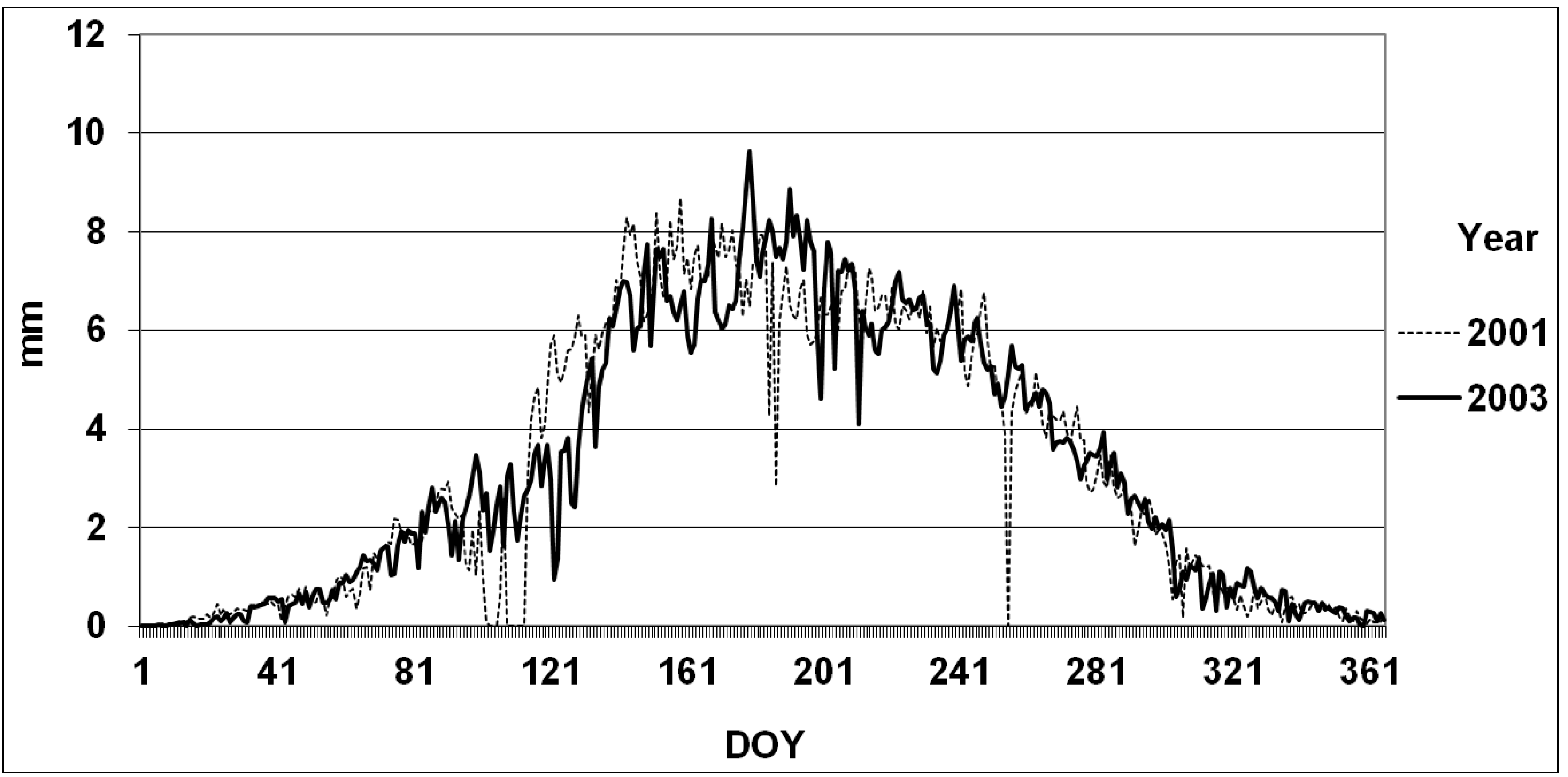
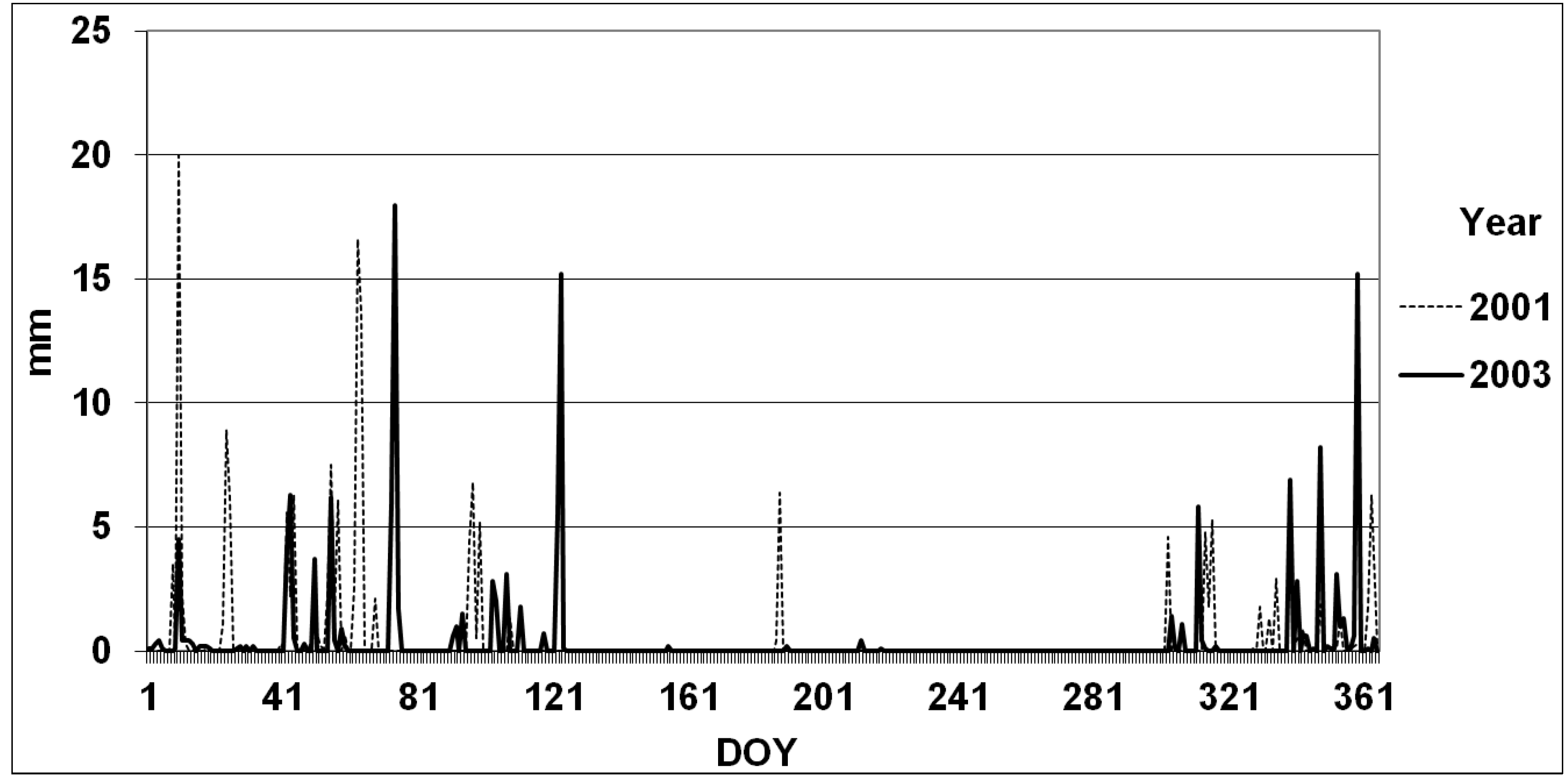
2.2.1. ETc and Soil Water Dynamics

Plant growth and plant uptake of water, salts and trace minerals are functions of ETc. ETc values were estimated using the corresponding ETo and crop Kc values developed using data from field measurements in 2007 (Equation 1). Estimated ETc values for 2001 and 2003 are shown in Figure 1.
Figure 1. Predicted ETc (mm) for Bermuda grass at the study site in 2001 and 2003 (DOY: day of the year).
Sustainability 05 03839 g001
Rainfall in 2001 and 2003 was 180.4 mm and 142.6 mm respectively (Figure 2).
Figure 2. Rainfall distribution (mm) at the study site in 2001 and 2003 (DOY: day of the year).
Sustainability 05 03839 g002
The amount and quality of the irrigation water applied to the research site varied between the years. In 2001 the pasture received 6 irrigations for a total of 5,846 m3·ha−1 and in 2003 it received 9 irrigations for a total of 7,711 m3·ha−1. The average ECiw in 2001 was 12.7 dS·m−1 and in 2003 was 2.6 dS·m−1 (Table 2). The amount and quality of drainage water available for irrigation reflected changing management conditions and water availability on the rest of the cooperator’s farm.
Table 2. Amount and electrical conductance (ECiw) of irrigation water (IW) used at the experimental site in 2001 and 2003.
YearIW (m3·ha−1)Eciw (dS·m−1)YearIW (m3·ha−1)ECiw (dS·m−1)
2001 2003
5-Jun-011,4648.712-Apr8973.2
18-Jul-011,08614.423-May1,0454.9
2-Aug-0176811.521-Jun6551.5
24-Aug-011,09116.23-Jul7742.9
14-Sep-01854NM26-Jul1,0264.3
28-Sep-01583NM14-Aug1,0390.8
---------26-Aug1912.4
---------4-Sep7212.0
---------3-Oct1,3641.7
Source: Adapted from Corwin et al. [52].
Predicted water flow through the four soil layers in 2001 and 2003 are shown in Figure 3.
Figure 3. Predicted soil water content (m3·m−3) in 2001 (A) and 2003 (B) in the four soil layers 0.0–0.3, 0.3–0.6, 0.6–0.9, and 0.9–1.2 m (DOY: day of the year).
Sustainability 05 03839 g003
Rainfall occurred only in winter months. Irrigation events are marked by large peaks in the spring-fall period. Although the amount of irrigation applied in 2003 was greater than in 2001, the larger number of irrigation events in 2003 resulted in a smaller amount of water being applied per event, with correspondingly less runoff and drainage, and lower leaching fractions that year. In 2001 the volume of runoff and drainage predicted was 23.0% of the irrigation, but in 2003 was only 10.7%. In a previous work at the same study site Kaffka et al. [19] reported an equivalent drainage value in the order of 10% for 2003 based on monitoring tile drainage flows and irrigation amounts. The higher drainage volume predicted in 2001 can be explained by the higher amount of rainfall and initial soil water content that year. The leaching fractions predicted for 2001 and 2003 were 2.6 % and 1.2 % respectively.

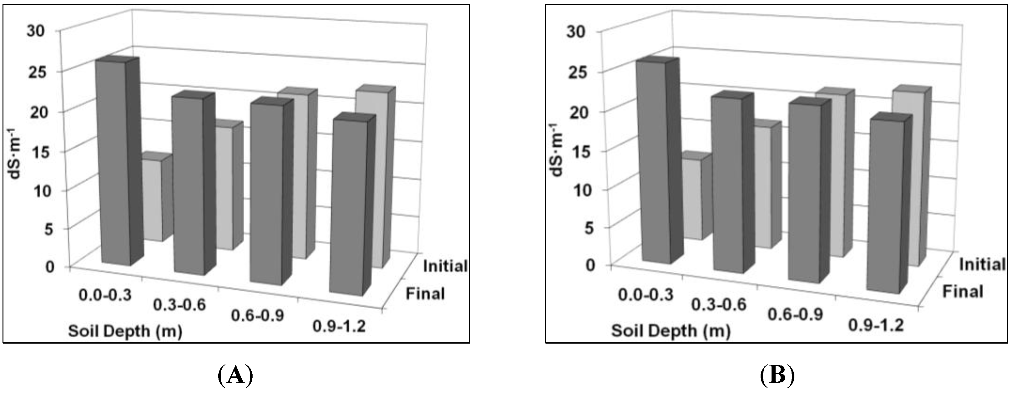
2.2.2 Soil Salinity Dynamics

The movement of salts (TDS, mg·L−1) in the soil is simulated as a function of the water flow through the profile. In 2001, due to a low leaching fraction and high ECiw, predicted ECe in the first two layers of the soil (0.0–0.3 and 0.3–0.6 m) increased at the end of the growing season. Predicted values at the start of the season were significantly lower (p < 0.05) than after the final irrigation in fall. The ECe of the two deepest layers did not vary significantly (p > 0.05) during the year (Figure 4). In 2003 soil salinity decreased after the growing season due to a larger amount of drainage water, a higher leaching fraction and a lower ECiw of the irrigation water (Figure 4). Modeled initial and final salinity values were significantly different (p < 0.05) for all the layers of the soil profile.
Figure 4. Predicted soil ECe (dS·m−1) before (initial) and after (final) the growing season at four different soil depths in 2001 (A) and 2003 (B).
Sustainability 05 03839 g004
The model matches observations from the research site summarized in Corwin et al. [52], who reported data collected on soil chemical properties at the field site between 1999 and 2004. Over this period, irrigation using mixed water quality ranging from 0.6 to 16.2 dS·m−1 resulted in an overall decline in salinity in the upper 1.2 m of the soil profile.

2.2.3. Soil Trace Minerals Dynamics

The concentration of trace minerals in the irrigation water at the research site varied between 2001 and 2003 (Table 3).
Table 3. Trace minerals in the irrigation water in 2001 and 2003.
YearB (mg·L−1)Se (µg·L−1)Mo (µg·L−1)
200115.1700400
2003230160
Source: Adapted from Corwin et al. [52].
The variability in the concentration of trace minerals in the soil at the study site was also large. Mean, minimum and maximum values of B, Se and Mo in the soil at WLF in 1999 and 2004 are shown in Table 4.
Table 4. Trace minerals averaged over 1.2 m in the soil at the study site in 1999 and 2004.
19992004
MeanMinMaxSDMeanMinMaxSD
B (mg·L−1)17.91.142.56.214.11.337.27.0
Se (μg·L−1)12.50.077.011.171.30.0704.0132.8
Mo (μg·L−1)835.1180.03,043.0438.1371.80.02,484.0368.8
Source: Adapted from Corwin et al. [52].
This data encompasses the time period of our study and coincides with crop sampling. Samples were collected at the soil sample sites identified in Corwin et al. [52]. When using the average values of trace minerals in the irrigation water reported by Corwin et al. [52], the model predicted a concentration of 13.78 mg·L−1 of B, 134.5 μg·L−1 of Se and 453μg·L−1 of Mo in the soil in 2001. Predicted values of B, Se and Mo in the soil in 2003 were 11.01 mg·L−1, 86.5 μg·L−1 and 173 μg·L−1 respectively. Predicted values of trace minerals in the soil in 2001 and 2003 are within the range of observed values at the field [52], but lower than the mean values. The explanation for this could be a non-uniform dilution of trace minerals in the water that flows out of the real system. The model assumes uniformity.

2.2.4. Forage Yield

Yield predictions for 2001 and 2003 were compared with observed values at the field site (Figure 5). Under field conditions the maximum yield predicted in 2001 is 7,090 kg DM·ha−1. The observed yield at the site on that year is 7,050 kg DM·ha−1. Predicted and observed values for 2003 are 4,320 kg DM·ha−1 and 4,480 kg DM·ha−1 respectively.
Figure 5. Predicted and observed yield values for Bermuda grass at the experimental site in 2001 (A) and 2003 (B). Model predictions are based on field conditions at those years. 95% confidence intervals for the mean of the observations are indicated by the bars (DOY: day of the year).
Sustainability 05 03839 g005
The difference in yield between 2001 and 2003 is explained by the nitrogen level in the soil and irrigation water. Our soil data indicate an average of 60 mmol·L−1 of NO3 in 2001 and of 39 mmol·L−1 in 2003. Corwin et al. [52] reported a reduction in soil NO3 between 1999 (64 mmol·L−1) and 2004 (34 mmol·L−1). The same study also reported a NO3 content < 0.1 (meq·L−1) in the irrigation water on 2000, 2002 and 2003, but a NO3 content of 0.6 meq·L−1 in the irrigation water on 2001, which is equivalent to 217 kg NO3·ha−1.
Model predictions for Bermuda grass yield fall within the 95% confidence interval for the mean of observed values in both years, however samples in 2001 have high variability with a standard deviation ranging from 650 kg DM·ha−1 at day 152 to 2,288 kg DM·ha−1 at day 250. There was a very low stocking rate at the field site in 2001, and this contributed to an uneven accumulation of biomass in the pasture generating this higher standard deviation among the samples.

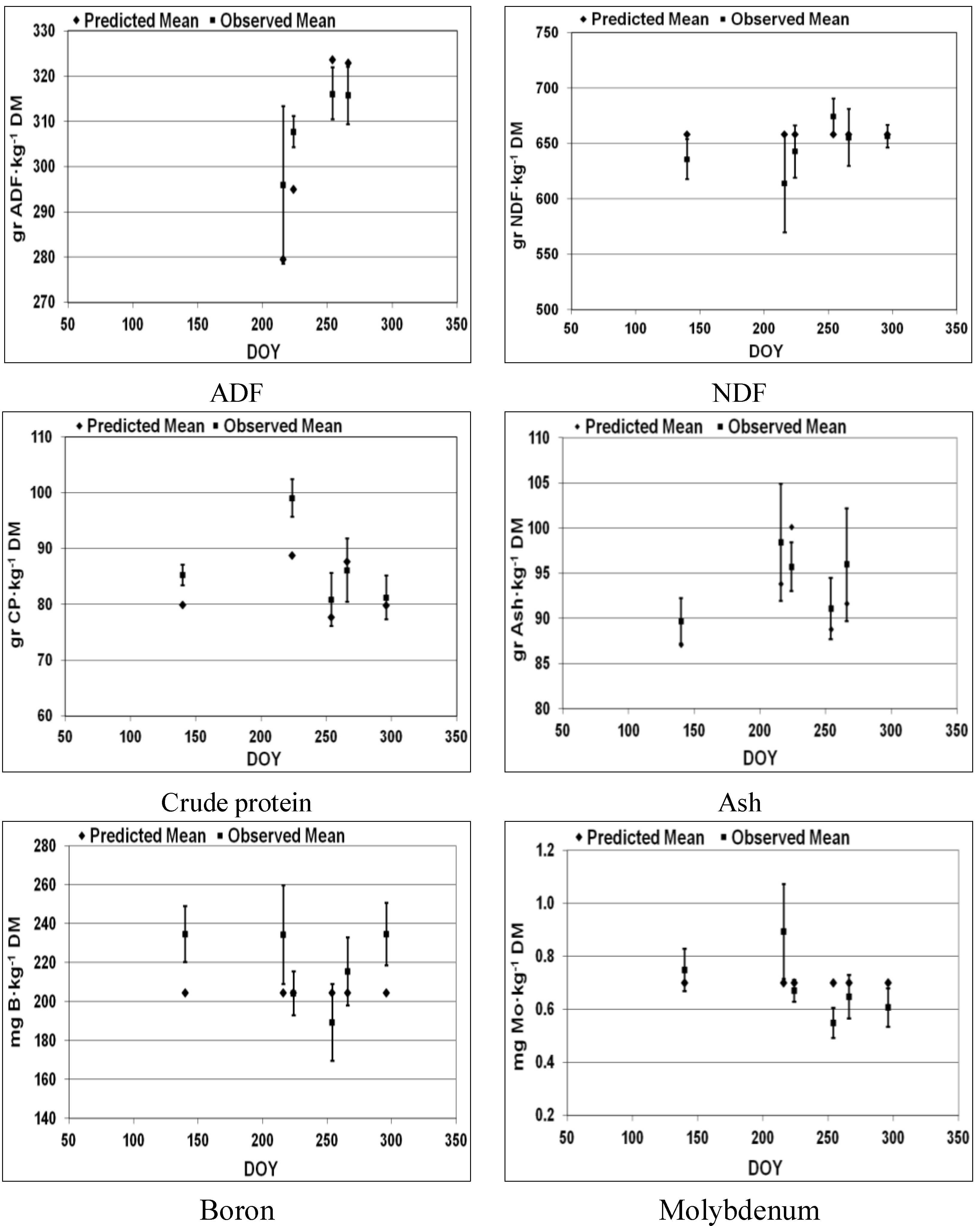
2.2.5. Forage Quality

The model fit for forage nutritional values is shown in Figure 6 and Table 5. In general, predicted values fall within the 95% confidence interval for the mean of observed values. There were more field observations of ADF, NDF, crude protein, ash, B and Mo in the forage in 2003 (Figure 6). On the other hand, there were more field observations of K, Ca, Mg and Se in the forage in 2001. Because of space constraints the model fit for K, Ca, Mg and Se is shown in a Table (Table 5).
Figure 6. Predicted and observed mean of acid detergent fiber (ADF), neutral detergent fiber (NDF), crude protein, ash, B and Mo in the forage in 2003. 95% confidence intervals for the mean of the observations are indicated by the bars.
Sustainability 05 03839 g006
Table 5. Predicted and observed mean values of K, Ca, Mg and Se in 2001. Confidence intervals are contained by the upper and lower 95% observed means.
K
gr·kg−1 DM
Ca
gr·kg−1 DM
Mg
gr·kg−1 DM
Se
µg·kg−1 DM
Year200120012001200120012001200120012001
Day of the year171297171297171297171250297
Predicted Mean1.901.900.470.470.260.2670.3070.3070.30
Observed Mean2.141.550.580.510.260.1575.6891.6174.53
Std. Dev. Obs Mean0.170.240.070.040.020.0222.4828.5123.93
Upper 95% Obs Mean2.221.670.610.530.270.1681.34101.2680.15
Lower 95% Obs Mean2.061.440.550.490.250.1470.0281.9668.91
Observations202020202020633672

2.2.6. Stocking Rate and Average Daily Gain

Average daily gains (ADG) for steers rotationally grazing at the experimental site in 2001 and 2003 are shown in Table 6. Predicted ADG’s for similar stocking rates range between 0.43 and 0.66 kg·day−1 in 2001 and between 0.53 and 0.83 kg·day−1 in 2003. Predicted values fall within the range of observed values in 2001 and 2003 considering grazing efficiencies between 40%–50% of the available biomass.
Table 6. Observed average daily gain (ADG) of steers grazing at the experimental site during the growing seasons 2001 and 2003.
YearGazing PeriodTreatmentSteersStocking RateADGSD
Days #AU·ha−1kg·day−1kg·day−1
2001143Control*80.50.560.09
143Treatment180.50.460.23
2003150Control100.60.550.15
150Treatment300.90.720.12
*: Control animals were supplemented with Cu and Se.

3. Results and Discussion

The validated model was used to estimate the system’s performance under likely combinations of irrigation amounts and frequencies, irrigation water salinity, fertilization and stocking rates that could occur in the WSJV.

3.1. Irrigation Management

Simulations with irrigation volumes of 80% ETc predicted 7,100 kg DM·ha−1, whereas irrigation volumes of 60% ETc yielded less than 6,500 kg DM·ha−1, at a fertilization rate of 300 kg N·ha−1. The model predicts that for the same total irrigation volume, yield increases between 4% and 8% when doubling the number of irrigation events. Dividing the total irrigation volume into a larger number of irrigations also decreases water loss to runoff and drainage. For seasonal irrigation applications equal to 80% ETc, increasing the irrigation frequency from one irrigation every 4 weeks to one irrigation every 2 weeks, starting on April 15th and ending on October 1st, water loses as runoff and drainage decrease from 46.4% to 10.2%. Simulations indicate, however, that there is a trade-off between water loss to runoff and drainage and the accumulation of salts in the profile, as predicted [58]. For the same irrigation volume, when increasing the number of irrigation events from a monthly to a biweekly basis, salt accumulation in the soil is on average 3.5 times higher when using irrigation water of 2.6 dS·m−1 ECiw, and 4.4 times higher when using irrigation water of 12.7 dS·m−1 ECiw, with soil ECe values at the end of the growing season ranging from 11.2 dS·m−1 for the highest drainage and leaching scenario to 25 dS·m−1 for the lowest one.

3.2. Fertilization Management

Crop response to N varies with salinity [54]. Simulated fertilization of 300 kg N·ha−1 increases predicted yield by 36% when irrigated with water of 2.6 dS·m−1, but only by 30% when irrigated with water of 12.7 dS·m−1. While a fertilized pasture (300 kg N·ha−1) yields 7,100 kg DM·ha−1, the maximum yield of Bermuda grass without fertilization is 4,300 kg DM·ha−1, both at 80% ETc and the range of ECe’s shown in Table 2.
Forage quality, including crude protein, ash and trace minerals was simulated. Crude protein in a fertilized pasture was 200.2 gr·kg−1 DM, but in an unfertilized one was 70.2 gr·kg−1 DM. The ash value in the forage ranged from 77 to 88.6 gr·kg−1 DM with and without fertilization respectively. Trace mineral accumulation interacts with N fertilization. On average, the concentrations of B, Mo and Se were close to 140 mg·kg−1 DM, 0.60 mg·kg−1 DM and 60 µg·kg−1 DM with N fertilization, and increased to 250 mg·kg−1 DM, 1.10 mg·kg−1 DM and 80 µg·kg−1 DM without it.

3.3. Grazing Management

Predicted stocking rates for steers gaining 0.5 kg·day−1 of body weight (BW) grazing the pasture during the growing season vary from 0.66 AU·ha−1 in a pasture without N fertilization to 1.66 AU·ha−1 in a pasture fertilized with 300 kg N·ha−1, both irrigated at 80% of ETc and with a grazing efficiency of 60%.
The level of trace minerals in forage is a concern when grazing pastures irrigated with drainage waters in saline areas. Even though there was a high concentration of trace minerals in the irrigation water applied at the field site in 2001, the concentration of trace minerals observed in the forage that year was below the maximum tolerable daily levels: 135 mg B·kg−1 BW; 12 mg Se·kg−1 BW; and 100 mg Mo·kg−1 BW [59].
A K/(Ca + Mg) ratio > 2.2 represents a risk of hypomagnesemic tetany for grazing cattle [60,61]. In our observation and simulations, this ratio naturally increases in fall for both fertilized and unfertilized pastures. The ratio also increases with fertilization and ECiw. Unfertilized pastures irrigated with low ECiw (2.63 dS·m−1) represent the lowest risk of tetany (ratio = 2.15). When the ECiw increases to 12.7 dS·m−1 the K/(Ca + Mg) ratio increases to 2.38. In fertilized pastures with low ECiw the average ratio is 3.78, but the same pastures irrigated with high ECiw present a ratio of 6.39, and a high risk of tetany. No tetany, however, was ever observed in grazing animals in the field over a ten year grazing period at the field site, including three years with direct observation and measurement.

3.4. System Performance

In general, model predictions fit data collected at the field site, with most predictions falling within 95% confidence intervals for the mean of observed values of forage yield, quality, and animal performance under grazing. Results of multiple simulations for different scenarios indicate the feasibility of growing Bermuda grass on the saline soils of the western San Joaquin Valley while managing the accumulation of salts and trace minerals in soils.
Soil chemical composition is highly affected by the amount and quality of the water used for irrigation during the growing season and to some extent can be managed through irrigation time and frequency. A combination of short, frequent irrigations to maximize crop yield and occasional long, deep irrigations to increase tile drainage and leaching of salts and trace minerals should be planned for each particular case. Precipitation and its influence on the dynamic of water, salts and trace minerals has to be accounted when making management decisions.
Related, small-scale trials [54] indicate that crop yields of 12 Mg DM·ha−1 are possible in these soils, although our simulations predict that a yield of 7 Mg DM·ha−1 is the most probable outcome if water volume, irrigation timing and quality restrictions are similar to those experienced at our field site at WLF, as described in Figure 2, Figure 3A, Figure 3B, and Table 2, Table 3, Table 4. Yields up to 4 Mg DM·ha−1 were observed and are predicted initially in unfertilized pastures when grazed. Without fertilization, these yields would decline over time.
The forage quality of a Bermuda grass pasture irrigated with marginal, saline drainage water in WSJV supported grazing. Observed and predicted forage ash values, critical when using forages growing on saline soils in animal diets, were on average less than 10% of forage DM. Trace minerals in the forage remained below maximum limits. The risk of hypomagnesemic tetany is a concern, especially when irrigating fertilized pastures with highly saline water. Our simulations indicate the end of the growing season to be the critical period. At this time, cattle should be closely observed and supplemented with magnesium when necessary.
A balance must be achieved among stocking rate, desired ADG, accumulation of salts in the soil profile and potential pollution of ground water due to run-off, drainage and leaching. Simulations show that it is possible to graze 1.0 to 1.2 AU·ha−1 without supplementation with gains of 1.0 kg·day−1 of live weight during the growing season, in an irrigated and fertilized Bermuda grass pasture located on saline soils in the WSJV. When the crop potential is reduced to 7 Mg DM·ha−1, the stocking rate should be reduced to 0.5 AU·ha−1 to allow a minimum weight gain of 0.5 kg·day−1 during the same period of time. At higher stocking rates, animals must be supplemented to sustain that rate of gain. If only weight maintenance is required, stocking rates could be increased to 1 AU·ha−1.
This model is useful for the analysis and management of Bermuda grass production and use in the WSJV of California. Using crop and site specific parameters [45] the model could be adapted to predict yield and quality of other grass species used for pasture or hay under saline conditions elsewhere in semi-arid regions where marginal soil and water resources are the only ones available.

4. Conclusions

We formulated a dynamic simulation model to organize a large set of empirical observations and data from a multi-year forage-livestock production system experiment. The model predicts Bermuda grass yield and quality, and beef cattle production in the western San Joaquin Valley of California. Crop-specific parameter values and functions were obtained in part from field observations and a related container trial to define water use coefficients. The model was validated by comparing predictions with observed crop, edapho-climatic and irrigation data from the field scale study site in Kings County, California. Results from observations of ongoing grazing at the site over the 2000–2011 period, and multiple simulations, indicate the feasibility of growing Bermuda grass for hay or grazing while managing soil salinity and trace minerals. A combination of short, shallow irrigations to match the availability of water in the soil with the water demand by the crop and long and deep irrigations or precipitation events to increase the leaching of salts and trace minerals provide flexibility of management. The model could be adapted for use by farmers growing forages on saline soils elsewhere based on available weather data, crop-specific parameter values and field scale measurements of soil salinity, trace minerals and nitrogen levels.

Acknowledgements

The authors acknowledge the California Department of Water Resources (contract # 4600004616) for funding part of the field work, the sample analyses and the modeling effort and the University of California’s Salinity Drainage Program for funding the container trial as well as original field site preparation, instrumentation and sample collection. The authors thank Ceil Howe III and Westlake Farms for the use of their land, and their efforts to provide and manage livestock, irrigation and other tasks at the research site.

Conflicts of Interest

The authors declare no conflict of interest.

References

  1. Swain, W.C. Estimation of Shallow Ground-Water Quality in the Western and Southern San Joaquin Valley, California; San Joaquin Valley Drainage Program: Sacramento, CA, USA, 1990. [Google Scholar]
  2. Wichelns, D.; Oster, J.D. Sustainable irrigation is necessary and achievable, but direct costs and environmental impacts can be substantial. Agr. Water Manage. 2006, 86, 114–127. [Google Scholar] [CrossRef]
  3. Tanji, K.K.; Lauchli, A.; Meyer, J. Selenium in the San Joaquin Valley. Environment 1986, 28, 6–11. [Google Scholar] [CrossRef]
  4. San Joaquin Valley Drainage Program, A Management Plan for Agricultural Subsurface Drainage and Related Problems on the Westside San Joaquin Valley; San Joaquin Valley Drainage Program: Sacramento, CA, USA, 1990.
  5. National Research Council, Soil and Water Quality: An Agenda for Agriculture: Committee on Long-Range Soil and Water Conservation, Board on Agriculture; The National Academies Press: Washington, DC, USA, 1993; p. 516.
  6. Shani, U.; Hanks, R.J. Model of integrated effects of boron, inert salt and water flow on crop yield. Agron. J. 1993, 85, 713–717. [Google Scholar] [CrossRef]
  7. Deverel, S.J.; Gilliom, R.J.; Fujii, R.; Izbicki, J.A.; Fields, J.C. Aerial distribution of selenium and other inorganic constituents in shallow ground water of the San Luis Drain Service Area, San Joaquin Valley, California: A preliminary study. Available online: http://pubs.usgs.gov/wri/1984/4319/report.pdf (accessed on 23 June 2013).
  8. Deverel, S.J.; Fujii, R. Processes affecting the distribution of selenium in shallow ground water of agricultural areas, western San Joaquin Valley, California. Water Resour. Res. 1988, 24, 516–524. [Google Scholar] [CrossRef]
  9. Deverel, S.J.; Millard, S.P. Distribution and mobility of selenium and other trace elements in shallow ground water of the western San Joaquin Valley, California. Environ. Sci. Technol. 1988, 22, 697–702. [Google Scholar] [CrossRef]
  10. Fujii, R.; Deverel, S.J. Mobility and distribution of selenium and salinity in groundwater and soil drained agricultural fields, Western San Joaquin Valley of California. In Selenium in Agriculture and Environment; Jacobs, L.W., Ed.; SSSA Special Publication: Madison, WI, USA, 1989; pp. 195–212. [Google Scholar]
  11. Van Schilfgaarde, J. Irrigation agriculture: Is it sustainable? In Agricultural Salinity Assessment and Management, ASCE Manu Report Practices; Tanji, K.K., Ed.; ASCE: Reston, VA, USA, 1990; pp. 584–594. [Google Scholar]
  12. Suttle, N.F. The interactions between copper, molybdenum, and sulphur in ruminant nutrition. Annu. Rev. Nutr. 1991, 4, 121–140. [Google Scholar] [CrossRef]
  13. Fujii, R.; Swain, W.C. Aerial distribution of selected trace elements, salinity, and major ions in shallow ground water, Tulare Basin, Southern San Joaquin Valley, California. Available online: http://wwwrcamnl.wr.usgs.gov/Selenium/Library_articles/FujiiSwain_text.pdf (accessed on 23 June 2013).
  14. Oster, J.D.; Grattan, S.R. Drainage water reuse. Irrigation Water Syst. 2002, 16, 297–310. [Google Scholar] [CrossRef]
  15. Schoups, G.; Hopmans, J.W.; Young, C.A.; Vrugt, J.A.; Wallender, W.W.; Tanji, K.K.; Panday, S. Sustainability of irrigated agriculture in the San Joaqin Valley, California. Proc. Natl. Acad. Sci. USA 2005, 102, 15352–15356. [Google Scholar]
  16. ANON. Grasslands Drainage Program. Available online: http://www-esd.lbl.gov/quinn/Grassland_Bypass/grasslnd.html (accessed on 23 June 2013).
  17. Skorupa, J.P. Selenium poisoning of fish and wildlife in nature: Lessons from twelve real-world examples. In Environmental Chemistry of Selenium; Frankenberger, W.T., Engberg, R.A., Eds.; Taylor & Francis: Abingdon, UK, 1998; pp. 315–334. [Google Scholar]
  18. Corwin, D.; Kaffka, S.R.; Oster, J.D.; Hopmans, J.W.; Mori, Y.; van Groenigen, J.-W.; van Kessel, C. Assessment and field-scale mapping of soil quality properties of a saline-sodic soil. Geoderma 2003, 114, 231–259. [Google Scholar] [CrossRef]
  19. Kaffka, S.R.; Oster, J.D.; Corwin, D.L. Forage production and soil reclamation using saline drainage water. In Proceedings of the National Alfalfa Symposium, San Diego, CA, USA, 13–15 December 2004; pp. 247–253.
  20. Robinson, P.H.; Grattan, S.R.; Getachew, G.; Grieve, C.M.; Poss, J.A.; Suarez, D.L.; Benes, S.E. Biomass accumulation and potential nutritive value of some forages irrigated with saline-sodic drainage. Anim. Feed Sci. Tech. 2004, 111, 175–189. [Google Scholar] [CrossRef]
  21. Grattan, S.R.; Grieve, C.M.; Poss, J.A.; Robinson, P.H.; Suarez, D.L.; Benes, S.E. Reuse of saline-sodic drainage water for irrigation in California: Evaluation of potential forages. In Proceedings of the 17th World Congress on Soil Salinity, Bangkok, Thailand, 14–21 August 2002; pp. 110–120.
  22. Grattan, S.R.; Grieve, C.M.; Poss, J.A.; Robinson, P.H.; Suarez, D.L.; Benes, S.E. Evaluation of salt-tolerant forages or sequential water reuse systems, I. Biomass production. Agr. Water Manage. 2004, 70, 109–120. [Google Scholar] [CrossRef]
  23. Grattan, S.R.; Grieve, C.M.; Poss, J.A.; Robinson, P.H.; Suarez, D.L.; Benes, S.E. Evaluation of salt-tolerant forages or sequential water reuse systems, III. Potential implications for ruminant mineral nutrition. Agr. Water Manage. 2004, 70, 137–150. [Google Scholar]
  24. Glen, E.P.; O’Leary, J. Relationship between salt accumulation and water content of dicotyledonous halophytes. Plant Cell Environ. 1984, 7, 253–261. [Google Scholar]
  25. Gorham, J.R.; Wyn Jones, G.; Macdonnell, E. Some mechanisms of salt tolerances in crop plants. Plant Soil 1985, 89, 15–40. [Google Scholar] [CrossRef]
  26. Glen, E.P. Relationship between cation accumulation and water content of salt tolerant grasses and sedge. Plant Cell Environ. 1987, 10, 205–212. [Google Scholar]
  27. Pessarakli, M.; Szabolcs, I. Soil Salinity and Soil Sodicity as Particular Plant/Crop Stress Factors; Pessarakli, M., Ed.; CRC press: Boca Raton, FL, USA, 1999. [Google Scholar]
  28. Zurayk, R.A.; Khoury, N.F.; Talhouk, S.N.; Baalbaki, R.Z. Salinity-heavy metal interactions in four salt-tolerant plant species. J. Plant Nutr. 2001, 24, 1773–1786. [Google Scholar] [CrossRef]
  29. Jones, C.A. C4 Grasses and Cereals: Growth, Development and Stress Response; John Wiley & Sons: New York, NY, USA, 1985. [Google Scholar]
  30. Maas, E.V.; Hoffman, G.J. Crop salt tolerance-current assessment. J. Irrigat. Drain. Div. 1977, 103, 115–134. [Google Scholar]
  31. Mitchell, R.L.; McLaren, J.B.; Fribourg, H.A. Forage growth, consumption, and performance of steers grazing Bermuda grass and Fescue Mixtures. Agron. J. 1986, 78, 675–680. [Google Scholar] [CrossRef]
  32. Overman, A.R.; Angley, E.A.; Wilkinson, S.R. Evaluation of an empirical model of coastal Bermuda grass production. Agr. Syst. 1988, 28, 57–66. [Google Scholar] [CrossRef]
  33. Overman, A.R.; Angley, E.A.; Wilkinson, S.R. A phenomenological model of Coastal Bermuda grass production. Agr. Syst. 1989, 29, 137–148. [Google Scholar]
  34. Overman, A.R.; Neff, E.; Wilkinson, S.R.; Martin, F.G. Water, harvest interval and applied nitrogen effects on forage yield of Bermuda grass and Bahia grass. Agron. J. 1990, 82, 1011–1016. [Google Scholar] [CrossRef]
  35. Overman, A.R.; Wilkinson, S.R. Partitioning of dry matter between leaf and stem in coastal Bermuda grass. Agr. Syst. 1989, 30, 35–47. [Google Scholar] [CrossRef]
  36. Overman, A.R.; Wilkinson, S.R. Model evaluation for perennial grasses in the southern United States. Agron. J. 1992, 84, 523–529. [Google Scholar] [CrossRef]
  37. Franzluebbers, A.J.; Wilkinson, S.R.; Stuedeman, J.A. Bermuda grass management in the Southern Piedmont USA: X. Costal productivity and persistence in response to fertilization and defoliation regimes. Agron. J. 2004, 96, 1400–1411. [Google Scholar] [CrossRef]
  38. Haby, V.A.; Stewart, W.M.; Leonard, A.T. Tifton 85 Bermuda grass response to Potasium sources and Sulfur. BC 2007, 91, 3–5. [Google Scholar]
  39. Silveira, M.L.; Haby, V.A.; Leonard, A.T. Response of Coastal Bermuda grass yield and nutrient uptake efficiency to nitrogen sources. Agron. J. 2007, 99, 707–714. [Google Scholar] [CrossRef]
  40. Kaffka, S.R.; Oster, J.D.; Corwin, D.L. Using forages and livestock to manage drainage water in the San Joaquin Valley. In Proceedings of the 17th World Congress on Soil Salinity, Bangkok, Thailand, 14–21 August 2002; pp. 1–12.
  41. Grieve, C.M.; Poss, J.A.; Grattan, S.R.; Suarez, D.L.; Benes, S.E.; Robinson, P.H. Evaluation of salt-tolerant forages for sequential water reuse systems II. Plant-ion relations. Agr. Water Manage. 2004, 70, 121–135. [Google Scholar]
  42. Masters, D.G.; Benes, S.E.; Norman, H.C. Biosaline agriculture for forage and livestock production. Agr. Ecosyst. Environ. 2007, 119, 234–248. [Google Scholar] [CrossRef]
  43. Suyama, H.; Benes, S.B.; Robinson, P.H.; Getachew, G.; Grattan, S.R.; Grieve, C.M. Biomas yield and nutritional quality of forage species under long-term irrigation with saline-sodic drainage water: Field evaluation. Anim. Feed Sci. Tech. 2007, 135, 329–345. [Google Scholar] [CrossRef]
  44. Suyama, H.; Benes, S.B.; Robinson, P.H.; Grattan, S.R.; Grieve, C.M.; Getachew, G. Forage yield andquality under irrigation with saline-sodic drainage water: Greenhouse evaluation. Agr. Water Manage. 2007, 88, 159–172. [Google Scholar] [CrossRef]
  45. Alonso, M.F.; Kaffka, S.R. Predicting water use, crop growth and quality of Bermuda grass under saline irrigation. Available online: http://www.water.ca.gov/drainage/docs/FinalReport_DWR_Kaffka.pdf (accessed on 23 June 2013).
  46. Overman, A.R.; Scholtz, R.V., III. Mathematical Models of Crop Growth and Yield; Marcel Dekker Inc.: New York, NY, USA, 2002; p. 328. [Google Scholar]
  47. Tanji, K.K. Nature and extent of agricultural salinity. In Agricultural Salinity Assessment and Management; ASCE: Reston, VA, USA, 1990; pp. 1–17. [Google Scholar]
  48. Pitman, M.G.; Lauchli, A. Global impact of salinity and agricultural ecosystems. In Salinity: Environment—Plants—Molecules; Lauchli, A., Luttge, U., Eds.; Kluwer Academic Publishers: Dordrecht, The Netherlands, 2002; pp. 3–20. [Google Scholar]
  49. United States Department of Agriculture, Soil Survey of Kings County, California; U.S. Government Printing Office: Washington, DC, USA, 1986.
  50. Lesch, S.M.; Rhoades, J.D.; Corwin, D.L. ESAP-95 Version 2.01R, User and Tutorial Guide; Brown, G.E., Jr., Ed.; US Salinity Laboratory: Riverside, CA, USA, 2000; p. 161. [Google Scholar]
  51. Corwin, D.L.; Lesch, S.M.; Oster, J.D.; Kaffka, S.R. Monitoring management-induced spatio-temporal changes in soil quality through soil sampling directed by apparent electrical conductivity. Geoderma 2006, 131, 369–387. [Google Scholar] [CrossRef]
  52. Corwin, D.L.; Lesch, S.M.; Oster, J.D.; Kaffka, S.R. Short-term sustainability of drainage water reuse: Spatio-temporal impact on soil chemical properties. J. Environ. Qual. 2008, 37, S8–S24. [Google Scholar]
  53. Snyder, R. SR-Excel: An Excel Application Program to Compute Surface Renewal Estimates of Sensible Heat Flux; University of California: Davis, CA, USA, 2008. [Google Scholar]
  54. Alonso, M.F.; Kaffka, S.R. Bermuda grass (Cynodon dactylon (L.)Pers.) yield and quality under different levels of salinity, nitrogen and trace elements: A container trial evaluation. Sustainability 2013, in press. [Google Scholar]
  55. ISEE Systems. Stella 9.0. 2006. Available online: http://www.iseesystems.com/ (accessed on 23 June 2013).
  56. Ben-Asher, J. Simplified model of integrated water and solute uptake by salts and selenium accumulating plants. Soil Sci. Soc. Am. J. 1994, 58, 1012–1016. [Google Scholar] [CrossRef]
  57. National Research Council, Nutrient Requirements of Beef Cattle, 7th ed.The National Academies Press: Washington, DC, USA, 2000; p. 248.
  58. Ayers, R.S.; Westcot, D.W. Water Quality for Agriculture; FAO: Rome, Italy, 1976. [Google Scholar]
  59. National Research Council, Mineral Tolerance of Animals: Second Revised Edition; The National Academies Press: Washington, DC, USA, 2005; p. 510.
  60. Grunes, D.L.; Stout, P.R.; Brownell, J.R. Grass tetany of ruminants. Adv. Agron. 1970, 22, 331–374. [Google Scholar] [CrossRef]
  61. Grunes, D.L.; Welch, R.M. Plant contents of magnesium, calcium and potassium in relation to ruminant nutrition. J. Anim. Sci. 1989, 67, 3485–3494. [Google Scholar]

