An Exergy-Based Model for Population Dynamics: Adaptation, Mutualism, Commensalism and Selective Extinction


Abstract
:List of Symbols
| aji | Discharge from “j” used by “i” |
| ci | Minimum consumption for survival of “i”, W |
| Ė | Exergy flow rate, W |
| Ėwi | Exergy flow rate discharged by “i”, W |
| Ėδi | Exergy flow rate destroyed by “i”, W |
| N | Population numerosity |
| pi | Global discharge coefficient of “i” |
| ri | Limit growth rate (births-deaths) of “i”, 1/y |
| wi | Exergy discharge coefficient of “i” |
Greek symbols
| βi | Dimensionless exergy capture coefficient of “i” |
| γi | Inflow capture coefficient, W/person of “i” |
| δi | Exergy destruction coefficient of “i” |
 i i | Coupling terms in Equation (7), W/person |
| θ | Parameter in Equation (15) |
| λi | Lyapunov exponents, 1/y |
| μi | Intrinsic mortality rate of “i”, 1/y |
1. Introduction
- a) An ad hoc approach that focuses on the particular dynamics of a single species or of a particular, generally small, ecological niche: models of such kind strongly depend on a set of very stringent initial assumptions, but thanks to their “specificity” have enjoyed a remarkable degree of success in reproducing experimental field data and—to a lesser extent—to predict future trends;
- b) The opposite approach is also possible: one tries to understand the population dynamics in a global sense, emphasizing and exploiting similarities in the behavior of different species in different environmental conditions and within different trophic chains. An original model of this second type has been proposed in previous papers by the present authors [4,5], and is based on the generally accepted principle that population dynamics depend substantially on the availability of primary resource and on the axiom that the consumption of such resources can be measured by an environmental indicator called extended exergy, EE in the following [6]. Extended Exergy is a physical quantity (measured in J, its fluxes in W) that explicitly measures the different forms in which natural resources are “available”, has the logical attributes of a “cost”, and thus is amenable to a resource accounting procedure -the method in fact goes under the name of Extended Exergy Accounting, EEA. Extended exergy is additive, explicitly includes irreversible losses, and its formulation covers the so-called “externalities”: using a somewhat anthropological expression, it can be rightly said that the EE of a commodity is a measure of the biosphere “effort” to convert low-entropy into high-entropy resources while generating that commodity. (Note: The conceptual novelty of Extended Exergy is its inclusion of the equivalent Capital, Labor and Environmental Remediation costs into the exergy “embodied” in a product of whatever material- or energy conversion chain. In the context of this paper, Capital and Labor are of course absent, and the difference between the use of exergy and extended exergy consists in the inclusion in the latter of the amount of natural exergy resources required of the environment to “biodegrade” the environmental damage produced by a species. To provide a simple example, the restoration of the trees destroyed by the Southern Pine Beetle [3] requires a certain amount of cumulative exergy, in the form of solar irradiation and nutrients, that represents the “cost” for the biosphere to recover its previous state. Similarly, the oxidation of pollutants in a water basin requires solar irradiation, microbic action, etc., all of which can be expressed in terms of “exergy inflow”).
- 1) The number N of individuals in a species at a given time depends on the global exergy resources a population can avail itself of.
- 2) These resources may be quantified in terms of Extended Exergy (i.e., by their primary resource equivalent), and expressed as a flux of exergy that each species may tap.
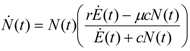
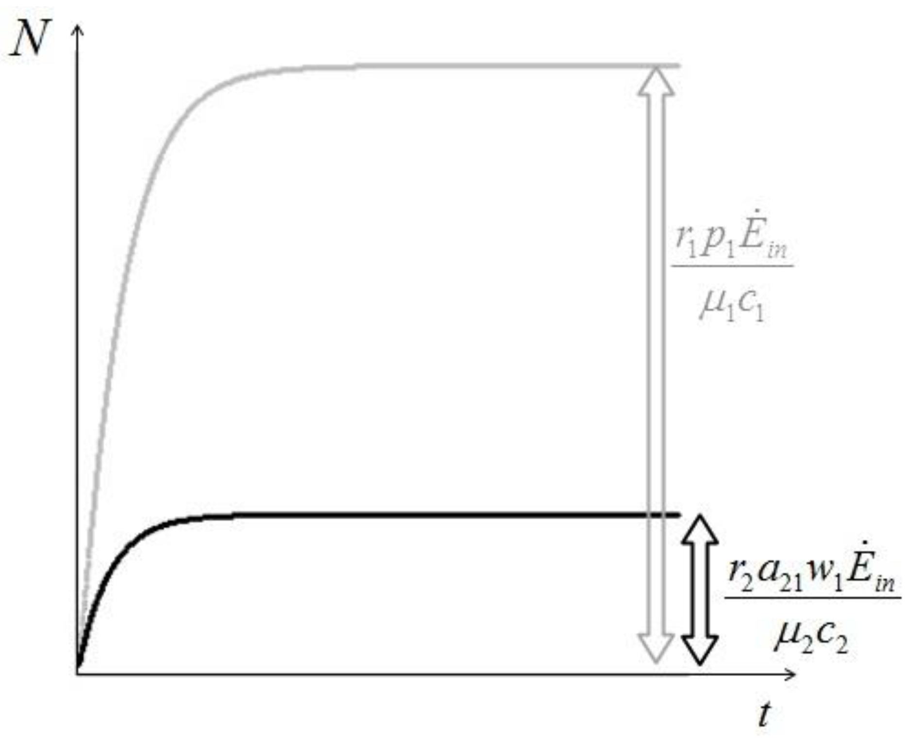
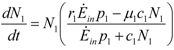
 . It is clear that as t → ∞, N(t) → N*. The behavior is indeed similar to that of a logistic-type equation under a carrying capacity constraint: here however the specific exergy consumption rate and the parameters of the model exactly define the carrying capacity. Note that in this case, under a constant influx condition (and therefore an infinite amount of cumulative exergy) at its disposal, the numerosity can sustain itself to the value N* for an infinite time. Obviously this is no longer true when
  describes a finite amount of cumulative exergy (see [4,5]). Notice also that the carrying capacity N* is proportional to Ė but also inversely proportional to c, a model constant representing the specific exergy consumption rate corresponding to“minimum survival” of the population; indeed if in a given interval of time the total energy consumption rate Ė(t) of the population is much higher than cN(t) then the population increases in that interval, while in the opposite situation the population would decrease: this means that the curve N(t) “follows” in some sense the curve Ė(t). A last remark: in the previous simple situation when Ė(t) is constant we can have two qualitative different behavior of the solution N(t) (see e.g. [4]): if at t = t0 the initial population size is larger than N*, then the population will monotonically (and exponentially) decrease to the value N*, while if the population size at t = t0 is smaller than N*, then the population will increase to the value N*. Some plots of the transient N(t) are provided in Figure 1: the gray curves represent the first case, the black ones the latter.
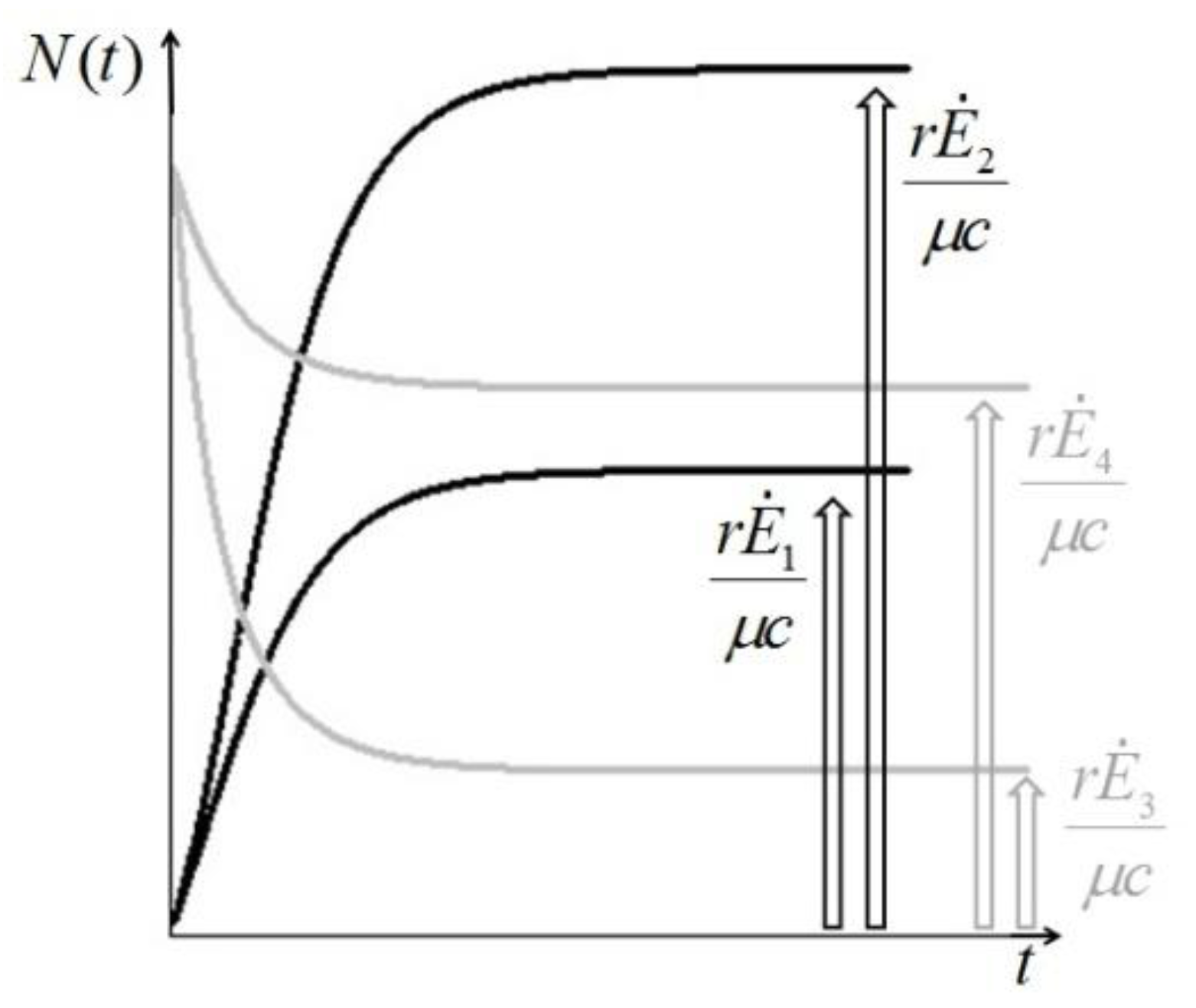
- a) Indifference: two species in the same environmental niche share the available incoming exergy flux but do not feed on each other’s discharges;
- b) Commensalism: one of the species survives solely on the resources released by its “host”;
- c) Mutualism; the two species compete for the externally available resources, but feed on each other’s discharges.
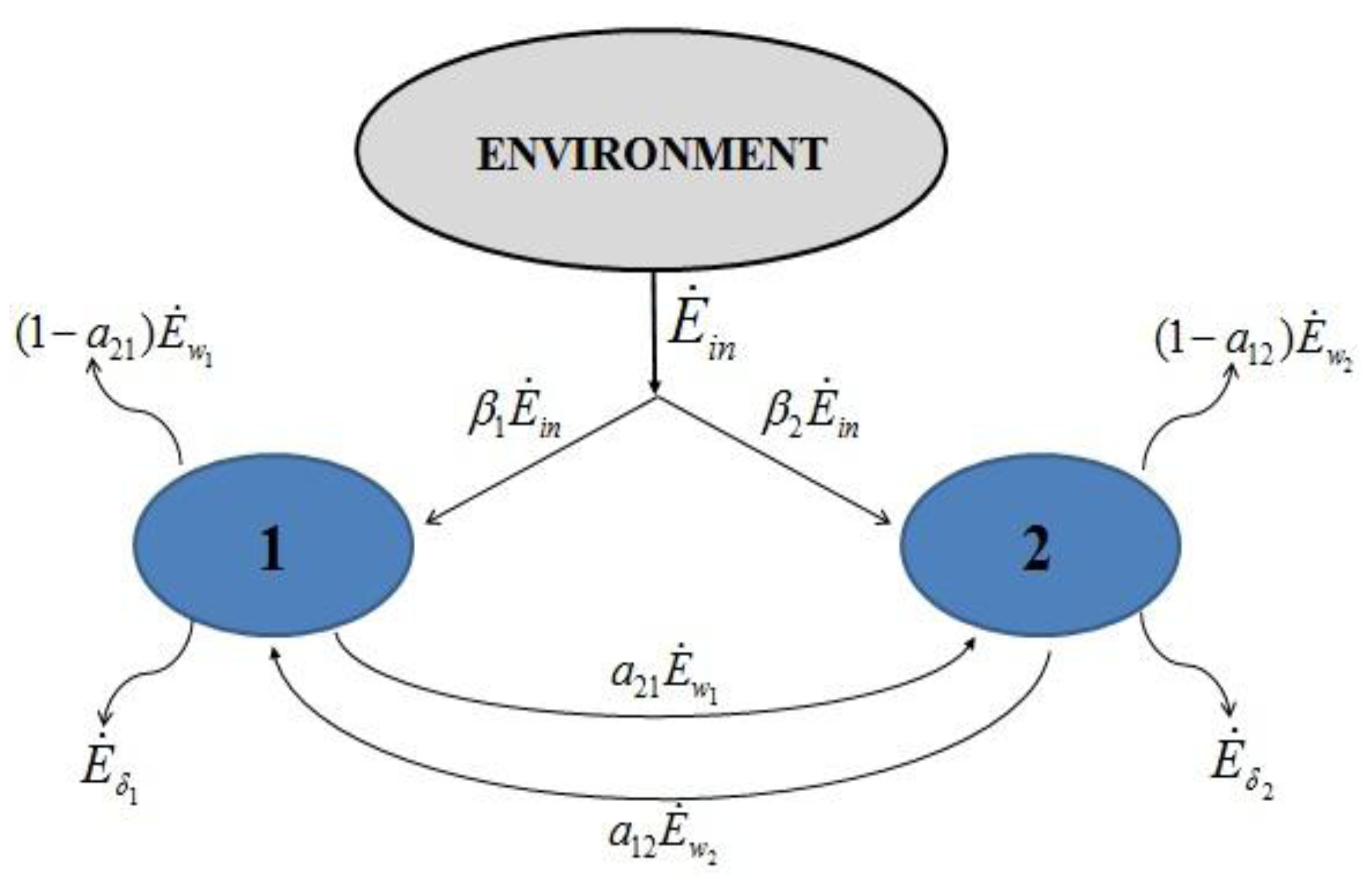
2. A Model of Two Interacting Populations Sharing a Common Renewable Resource


 and
and  , γ1 and γ2 (both in J/individual/day) being the specific exergy consumptions of the two species (notice that β1+β2=1 and that
  as requested by the imposed boundary conditions). In most real situations, the parameters γi could depend also on time: in this paper, for simplicity, we posit that they are constant. Note that the parameter ank is the amount of the discharge of species k “recycled” by species n: if ank=akn=0, the two populations are indifferent to each other, i.e., neither one exploits the discharges of the other as its own exergy input). Since the instantaneous rate of discharge and destruction of the exergy flow can be only a fraction of the incoming one, we set
  and
and  where wi and δi are two dimensionless species-specific constants measuring the portion of incoming flow being discharged and destroyed by population Ni: In the model presented here, these “discharges” are NOT equivalent to the detritus (which is a pure material flow rate): they include also any form of exergy released by species j (thermal, chemical, etc.)
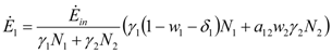
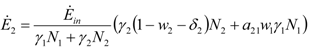
 and
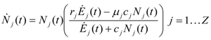
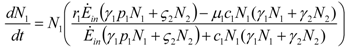
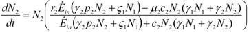
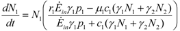
and  . The strong coupling between the numerosity of each species and the time evolution of ALL the participating species is apparent. Notice that in this case, Z = 2, but the formulae can be easily extended to account for whatever number Z of interacting populations, see [1]. We shall assume in the following that the exergy influx Ėin is constant and that the model coefficients γ, w, δ, r, μ and c are known for all species considered. The type and degree of interaction between the two species is represented by the terms k and γk that respectively contain the “βj” (that express the exergy voracity of species j) and the “αij,” that quantify the degree of mutualism. Let us examine, on the same line as proposed in [8], the three possible general behaviors. Notice that Jørgensen [8] uses “cooperation” and “parasitism” to indicate “mutualism” and “commensalism” respectively.
2.1. Indifference
 and
and  . These two parameters contain the efficiency of each species to gain “net” exergy flows (γkpk), their “minimal survival” requests (ck) and the ratio of the growth rate to the mortality rate
  in the respective limit cases of infinite and zero resources available. For simplicity let us consider that > ; the symmetric results for > will simply follow by permutation of the indices 1 ↔ 2 , and the special case = will be discussed at the end of the section. In the state plane (N1, N2), the system of Equations 8 and 9 possesses three fixed points, listed in Table 1:
| N1 | N2 | |
| a) | 0 | 0 |
| b) | 0 |  |
| c) |  | 0 |
| λ1 | λ2 | |
| a) | r1 | r2 |
| b) |  |  |
| c) |  |  |
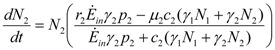
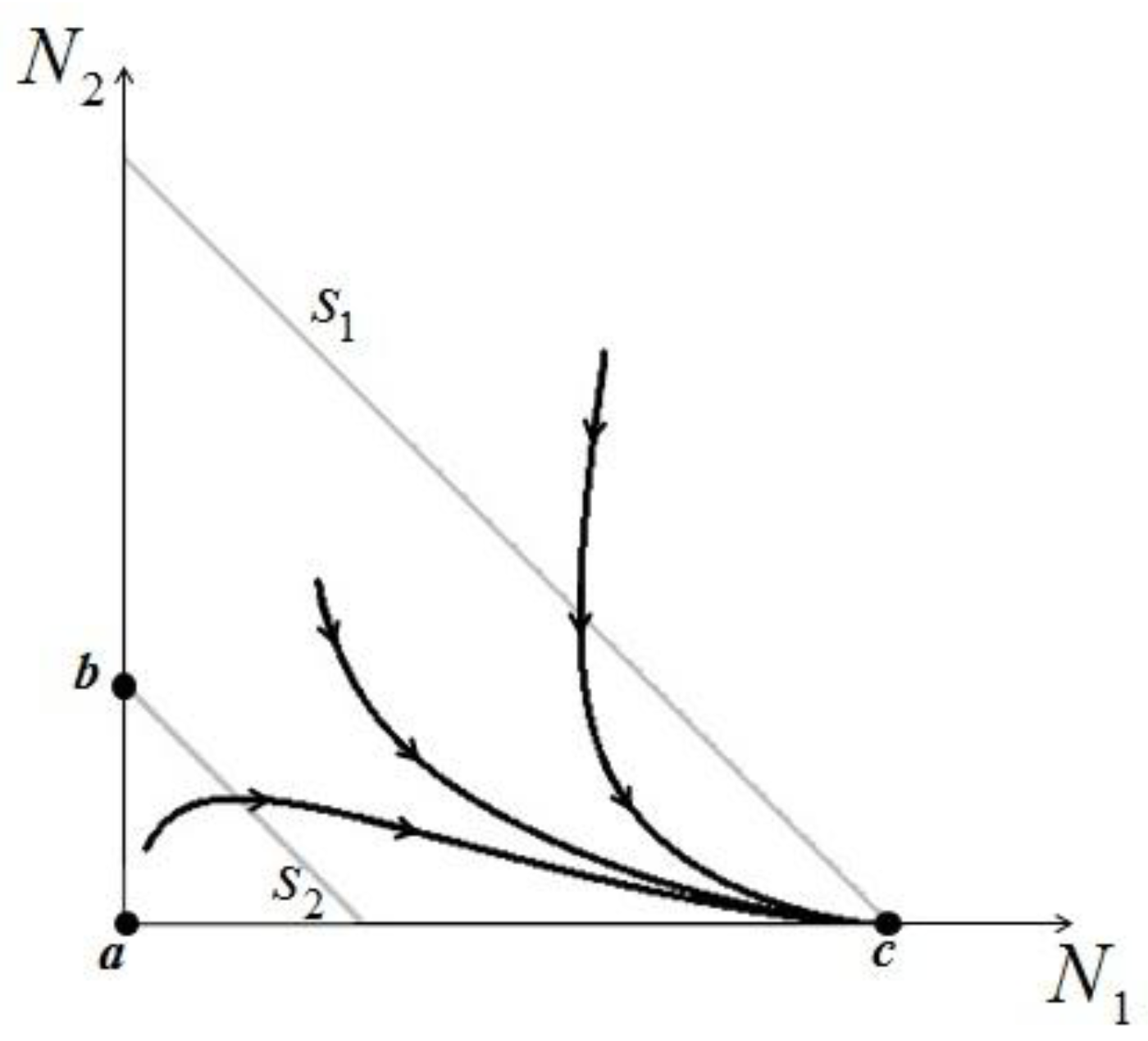
> results in point c being asymptotically stable and point b unstable. We can divide the plane (N1, N2) into three different regions (only the semi-plane defined by N1 ≥ 0 and N2 ≥ 0 are considered here because this semiplane is invariant under the flow). The three regions are divided by the so called isoclines s1 and s2, defined as (see Figure 3):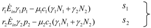
 1 = 0 and on s2, 2 = 0. Notice that the two lines have the same angular coefficient and, since here > , line s1 is above s2.
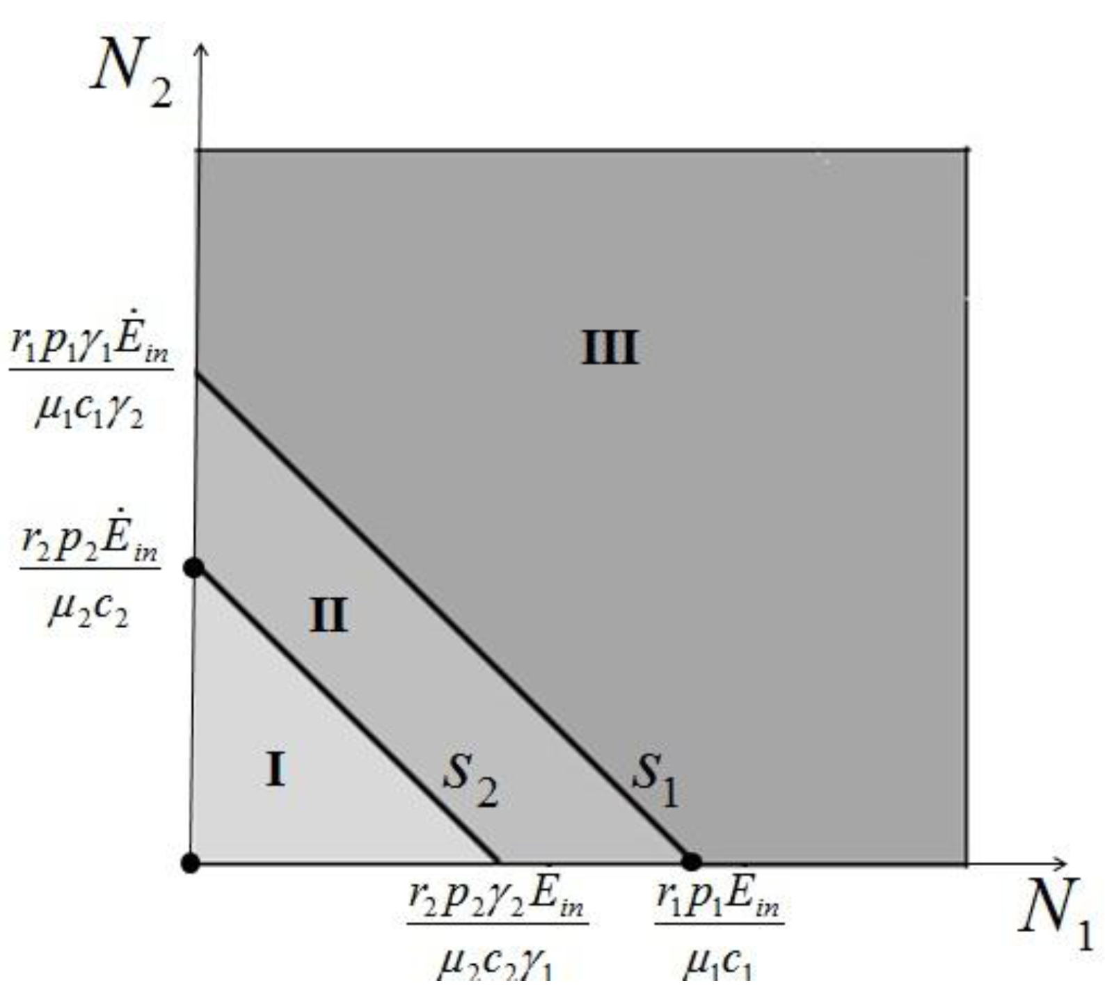 > is satisfied, population N2 will become extinct and population N1 will tend to the stable (sustainable) value . By the same arguments it can be shown that conversely, if < , population N1 will die out and population N2 reaches a stable limit . An ensemble of plots for the case > , corresponding to different initial conditions, is shown in Figure 4. > .
 = is very interesting. Point a is again unstable, but now the two isoclines s1 and s2 converge into a line that is itself an attractor. Both species survive and the weighted sum γ1N1 + γ2N2 reaches the carrying capacity limit for which
  . Figure 5 shows examples of possible behaviors in phase space.
  : The arrows indicate the time direction of the evolution.
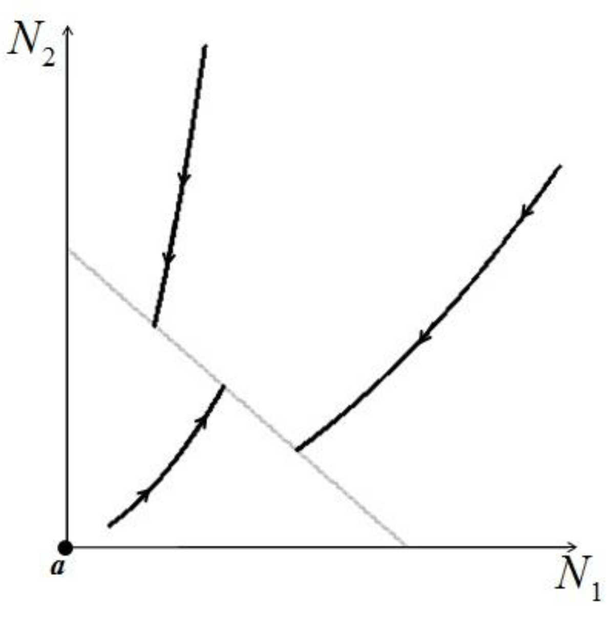
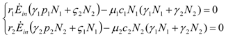
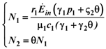
2.2. Commensalism
 1 and γ1: thus, the system (14) can be formally integrated, even if the solutions can be only written out implicitly:
 and
and  are given by:
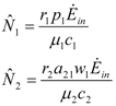
 and
and  . Thus, both species reach their respective carrying capacity limit. Note that
  is proportional to p1, i.e. to 1 − w1 − δ1: increasing the discharged and destroyed portion of the incoming exergy flows proportionally reduces the corresponding carrying capacity value for population 1. But population 2 feeds on this discharged flow: Equation 16 shows that indeed the carrying capacity limit for N2 is proportional to w1. Note that, in contrast to the case of competing populations, and assuming w1 ≠ 0, the two populations will always both survive. In fact, species 1 meets no competition in tapping the exergy flow it needs and species 2 feeds on the “crumbs” of species 1. This result is quite obvious, but we stress that:
 - a) it is derived on exact mathematical basis.
- b) the carrying capacity limits are directly linked to the parameters of the model.
- c) Equations 14 describe also how fast these limits are reached (Figure 6).

2.3. Mutualism
| λ1 | λ2 | |
| a) | r1 | r2 |
| b) | r1 | |
| c) | | r2 |
 and
and  ):
):
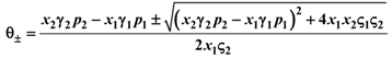
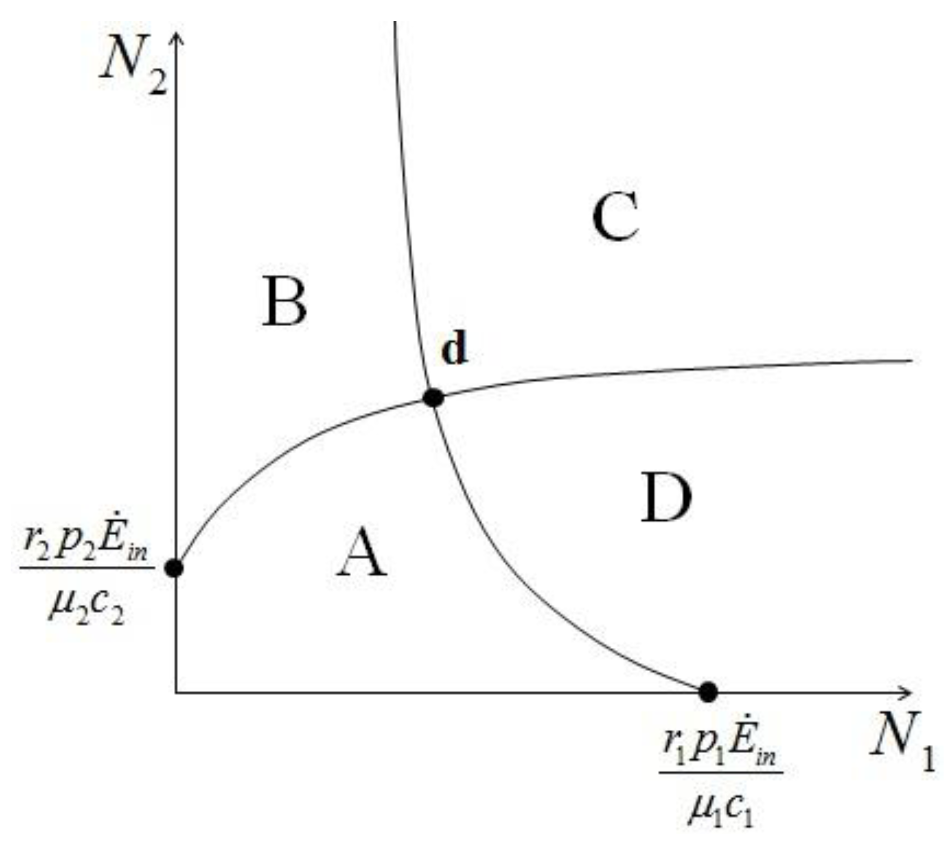
 1 and 2. Consider species 1 first. In order to have 1 ≥ 0 we need:
 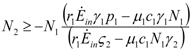 1 > 0, and region II, where 1 < 0. The two lines depicted in Figure 7 correspond to the two cases
  and
and  : the special case
  (and the equivalent case for species 2
  ) will be discussed at the end of this section. (left) and (right).
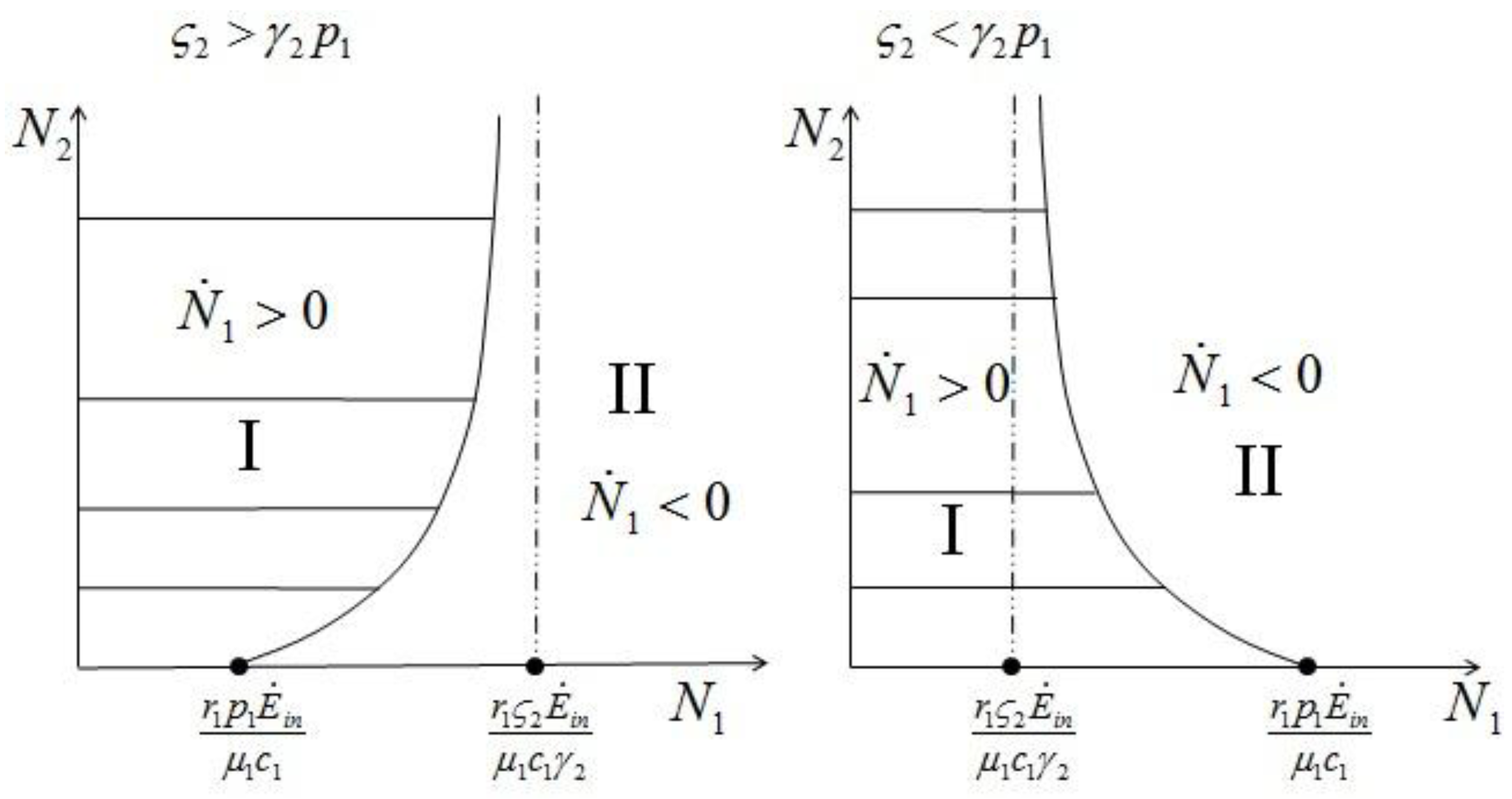
 and
and  :2 for (left) and .
 and , to find the fixed point d we can superimpose the two curves on the right in Figure 7 and Figure 8 to obtain the picture shown in Figure 9.
 1 and 2. In region A both 1 and 2 are positive, so N1 and N2 are both increasing functions of time. In region B N1 is increasing and N2 is decreasing. In region C N1 is decreasing and N2 increasing and finally in region D both N1 and N2 are decreasing functions of time. Thus, point d is attractive. The same argument applies for the other three possible cases ( , ), ( , ) and ( , ).
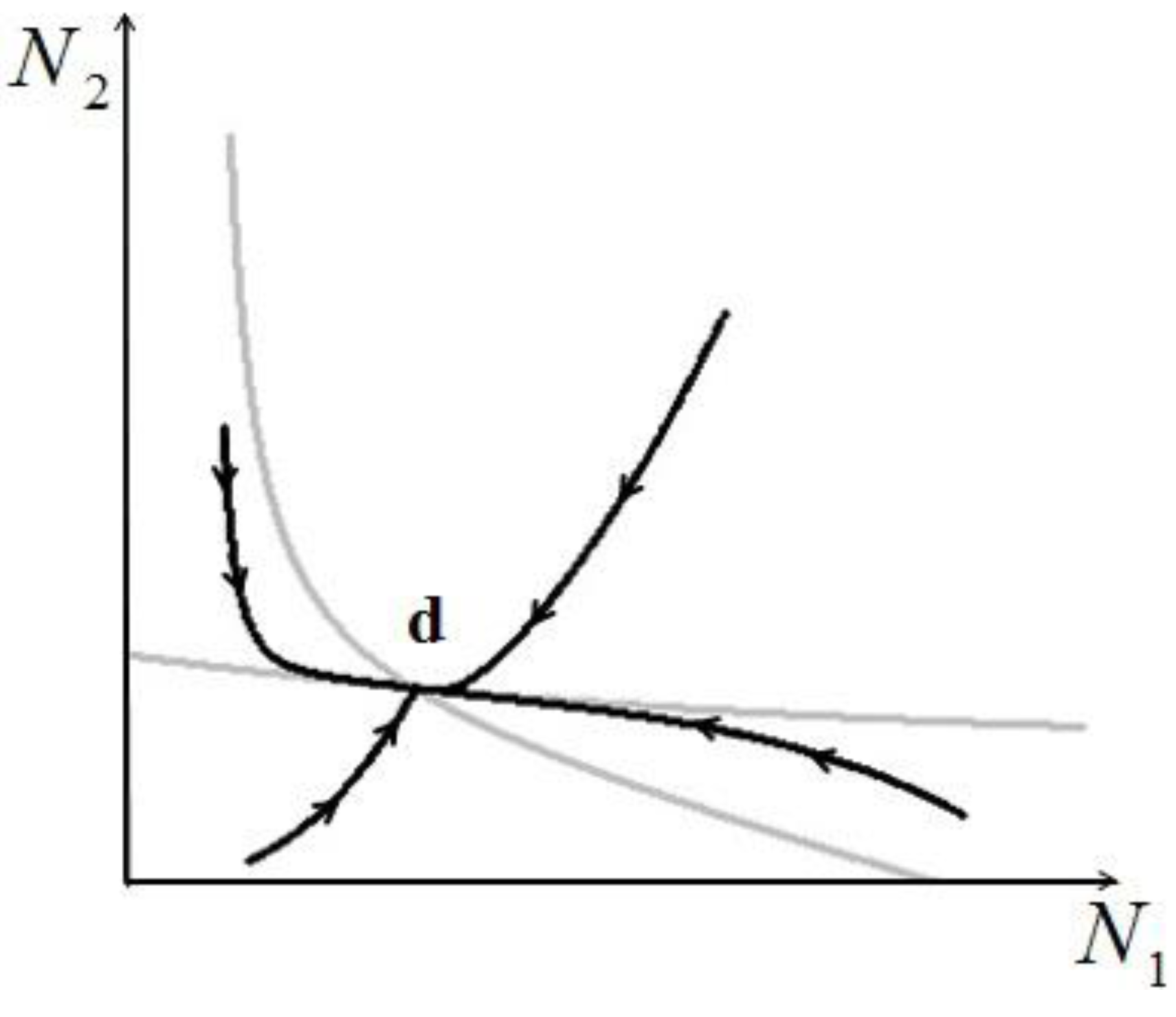
 is also independent of Ėin and depends only on the parameters characterizing the species and their interaction (competition-cooperation). From a mathematically point of view this property of the solution is tautologic, but the question of whether a real system actually possesses this attribute is indeed far from obvious: since the ratio and Ėin are easily measurable in field experiments, the above constraint is suggesting a possible experimental “check” on the model. In a future paper we plan to examine some of the available experimental result in order to verify whether this statement is falsifiable.. Looking at Figure 7 now the two points marked with black dots on the N1 axis coincide, so that the curve dividing the semi-plane into two regions becomes a straight line, and the intersection point is now given by:
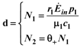
 , sum up just to Ėinp1. This is a rather special situation but it is interesting to note how the equation for N1 decouples. In contrast to the second of (15), however, the equation for 2 depends on both populations, so we cannot give analytical results as in that case. It is clear however that the qualitative dynamics cannot differ much from the general case.
 3. Conclusions
- − if the two species just coexist in the same niche without cooperating or preying on each other, their competition invariably leads (Section 2a) to the extinction of one of them, unless their genetic (r, μ), consumption (c, γ) and efficiency (p) parameters are in a very precise and delicately tuned balance, in which case the two species may coexist sustainably;
- − if one of the two species assumes a commensalistic type of behaviour (it feeds on the other’s discharges, Section 2b), then both species reach their respective carrying capacity limits;
- − if the two species display a mutualistic type of behaviour (each one feeds partially on the other’s discharges, Section 2c), then there is always a stable sustainable point and both populations survive.
- 1) Substitutability of exergy resources: our model explicitly lumps all of the “available” material and energy fluxes into the extended exergy inflow Ėin. This poses no problem for the energy flows, but contains the implicit assumption that ALL material flows are perfectly substitutable. In the simplest case, consider an animal species that has access to two or three different sources of vegetable food: obviously, each vegetable has a different nutritive value for the species, but also a different extended exergy content. Thus, our model would predict that the “optimal choice” for the animal would be to feed on the lower-embodied exergy food with the highest nutritive value. But this prediction disregards preferences, spatial distribution, physical accessibility, and similar factors. For more complex behaviours (for instance, related to the human species), the choice between, say, bronze and iron to build spears is even more multi-faceted than implicitly posited by the model.
- 2) Actual possibility of species reaching a stable stationary state: this is of course an extremely important point, because if two species in a single ecological niche reach a stable state (point d in Figure 10), this is by definition a sustainable situation. For larger number of species and realistic conditions, the problem of the stability of such stationary states is of paramount importance, and has not been addressed here.
- 3) Metadynamics: the model presented in this paper is spatially lumped and the niche in which the species thrive has “impermeable boundaries”. Immigration and emigration are completely neglected, as well as spatially varying distributions of Ėin. While the former could be modeled by inserting an “immigration term” in Equations (6) and (7), the spatially lumped nature of the model is difficult to modify. One solution might be that of “discretizing” the domain, and apply the equations separately to different areas, accounting for the variation of Ėin in each subdomain. This would make our model somewhat comparable to the so-called “patch” [10] or “incidence function” models [11], but would also demand for very taxing numerical simulations, not considered here.
- 4) Limiting factors (“exogenous factors” in [3]): while we maintain that (extended) exergy is a satisfactory indicator of species numerosity (in the sense that high exergy niches must logically and thermodynamically correspond to globally higher numerosities), it must be remarked that in real ecological niches there are phenomena occurring at some scales that affect the numerosity of species at a different scale [12]. Viral and fungal infections to which species N is insensitive may affect one or more of its food sources; growth of high-foliage trees with which a vegetable species does not compete for nutrients may reduce its share of solar irradiation, etc.: at the present state of development it is not clear whether and how our model may accommodate such effects (like in “tritrophic” or “multi-trophic” models [3]).
- 5) Though not addressed in this paper, the application of our model raises a question that could be of paramount importance for practical applications: is the efficiency of one single species in the niche compatible with the overall energy-conversion efficiency of the same niche, considered as a lumped system? In other words, if two or more species reach a sustainable point (“d” in Figure 10), do their respective numerosities satisfy both a local (for each species) and a global (for the entire niche) “optimal exergy use” criterion? This is a topic we have left for a future study.
Acknowledgments
Conflict of Interest
Appendix 1
 and
and  . But in this region these functions are also increasing; they must approach asymptotically a limit, say the point (x = , ). This means that x is an equilibrium point. But the only equilibrium points are given in Table 1, and x cannot be any of these points since N1 and N2 are increasing functions. So the solution will leave the region I at some time t. 1(t*) = 0. For the second derivative of 1 at t = t* we have (since 2(t*) < 0):
 2(t*) = 0. The second derivative of N2 at t = t* is given by:
 1(t*) > 0. So N2 has a maximum at t = t*, but again this cannot be the case since N2 is a decreasing function in region II.
References
- Benton, T.G.; Plaistow, S.J.; Coulson, T.N. Complex population dynamics and complex causation: Devils, details and demography. Proc. R. Soc. B 2006, 273, 1173–1181. [Google Scholar] [CrossRef]
- Hanski, I. Metapopulation Dynamics; Oxford University Press: Oxford, UK, 1999. [Google Scholar]
- Turchin, P. Complex Population Dynamics: A Theoretical/Empirical Synthesis; Cambridge University Press: Cambridge, UK, 2003. [Google Scholar]
- Sciubba, E.; Zullo, F. Exergy-based population dynamics: A thermodynamic view of the “sustainability” concept. J. Ind. Ecol. 2011, 15, 172–184. [Google Scholar] [CrossRef]
- Sciubba, E.; Zullo, F. Is sustainability a thermodynamic concept? IJEX 2011, 8, 68–85. [Google Scholar]
- Sciubba, E. Beyond thermoeconomics? The concept of extended exergy accounting and its application to the analysis and design of thermal systems. IJEX 2001, 1, 68–84. [Google Scholar]
- Sciubba, E. What did Lotka really say? Ecol. Modelling 2009, 222, 1347–1353. [Google Scholar] [CrossRef]
- Jørgensen, S.E. Fundamentals of Ecological Modeling; Fath, B., Jørgensen, S.E., Eds.; Elsevier: Oxford, UK, 2011. [Google Scholar]
- Kareiva, P.; Mullen, A.; Southwood, R. Population dynamics in spatially complex environments: Theory and data and discussion. Phil. Trans. R. Soc. Lond. 1990, 330, 175–190. [Google Scholar]
- Diamond, J.M.; May, R.M. Island Biogeography and the Design of Natural Reserves. In Theoretical Ecology; May, R.M, Ed.; Blackwell Pub.: Oxford, UK, 1981; pp. 228–252. [Google Scholar]
- Durrett, R.; Levin, S. The importance of being discrete and spatial. Theoretical Popul. Bio. 1994, 46, 363–394. [Google Scholar] [CrossRef]
- Williamson, M. The Analysis of Biological Populations; Edward Arnold Pub.: London, UK, 1971. [Google Scholar]
© 2012 by the authors; licensee MDPI, Basel, Switzerland. This article is an open-access article distributed under the terms and conditions of the Creative Commons Attribution license (http://creativecommons.org/licenses/by/3.0/).
Share and Cite
Sciubba, E.; Zullo, F. An Exergy-Based Model for Population Dynamics: Adaptation, Mutualism, Commensalism and Selective Extinction. Sustainability 2012, 4, 2611-2629. https://doi.org/10.3390/su4102611
Sciubba E, Zullo F. An Exergy-Based Model for Population Dynamics: Adaptation, Mutualism, Commensalism and Selective Extinction. Sustainability. 2012; 4(10):2611-2629. https://doi.org/10.3390/su4102611
Chicago/Turabian StyleSciubba, Enrico, and Federico Zullo. 2012. "An Exergy-Based Model for Population Dynamics: Adaptation, Mutualism, Commensalism and Selective Extinction" Sustainability 4, no. 10: 2611-2629. https://doi.org/10.3390/su4102611