<?xml version="1.0" encoding="UTF-8"?>
<!DOCTYPE article PUBLIC "-//NLM//DTD Journal Publishing DTD v2.3 20070202//EN" "journalpublishing.dtd">
<article xmlns:mml="http://www.w3.org/1998/Math/MathML" xmlns:xlink="http://www.w3.org/1999/xlink" xml:lang="en" article-type="research-article">
<front>
<journal-meta>
<journal-id journal-id-type="publisher-id">Sustainability</journal-id>
<journal-title>Sustainability</journal-title>
<issn pub-type="epub">2071-1050</issn>
<publisher>
<publisher-name>Molecular Diversity Preservation International (MDPI)</publisher-name></publisher></journal-meta>
<article-meta>
<article-id pub-id-type="doi">10.3390/su3081114</article-id>
<article-id pub-id-type="publisher-id">sustainability-03-01114</article-id>
<article-categories>
<subj-group>
<subject>Article</subject></subj-group></article-categories>
<title-group>
<article-title>Risk Assessment and Examination of Economic Aspects of Precision Weed Management</article-title></title-group>
<contrib-group>
<contrib contrib-type="author">
<name><surname>Takács-György</surname><given-names>Katalin</given-names></name><xref ref-type="corresp" rid="c1-sustainability-03-01114"><sup>*</sup></xref></contrib>
<contrib contrib-type="author">
<name><surname>Takács</surname><given-names>István</given-names></name></contrib>
<aff id="af1-sustainability-03-01114">Károly Róbert College, Institute of Business and Organizational Management, H–3200 Gyöngyös, Mátrai út 36, Hungary; E-Mail: <email>itakacs@karolyrobert.hu</email></aff></contrib-group>
<author-notes>
<corresp id="c1-sustainability-03-01114">
<label>*</label> Author to whom correspondence should be addressed; E-Mail: <email>tgyk@karolyrobert.hu</email>; Tel.: +36-30-297-8674; Fax: +36-37-518-155.</corresp></author-notes>
<pub-date pub-type="collection">
<year>2011</year></pub-date>
<pub-date pub-type="epub">
<day>27</day>
<month>07</month>
<year>2011</year></pub-date>
<volume>3</volume>
<issue>8</issue>
<fpage>1114</fpage>
<lpage>1135</lpage>
<history>
<date date-type="received">
<day>15</day>
<month>04</month>
<year>2011</year></date>
<date date-type="rev-recd">
<day>01</day>
<month>07</month>
<year>2011</year></date>
<date date-type="accepted">
<day>08</day>
<month>07</month>
<year>2011</year></date></history>
<permissions>
<copyright-statement>© 2011 by the authors; licensee MDPI, Basel, Switzerland.</copyright-statement>
<copyright-year>2011</copyright-year>
<license>
<p>This article is an open access article distributed under the terms and conditions of the Creative Commons Attribution license (http://creativecommons.org/licenses/by/3.0/).</p></license></permissions>
<abstract>
<p>The aim of this research is to investigate plant production sustainability, the economical requirements, risks, and identify threshold levels to switching on, or off precision weed management techniques in Hungarian growing and sales conditions; taking into consideration that the implementation of precision technology can be justified also by its role in the reduction of environmental load, which would create a harmony between individual usefulness and social utility. A simulation model has been developed to investigate the return of extra investments, along with the risk of this return in relation to the soil type, weed coverage, and the sales price.</p></abstract>
<kwd-group>
<kwd>precision crop protection</kwd>
<kwd>switch</kwd>
<kwd>returns</kwd>
<kwd>modeling</kwd></kwd-group></article-meta></front>
<body>
<sec sec-type="intro">
<label>1.</label>
<title>Introduction</title>
<p>The objective of this current paper is to examine the economic relations and the consequences of precision weed control, as well as the risks of precision crop production.</p>
<sec>
<label>1.1.</label>
<title>How Can the Idea of Sustainability Benefit from Precision Farming?</title>
<p>Sustainability with regard to agricultural activity can be defined with the help of several definitions. In Pearce and Atkinson's [<xref ref-type="bibr" rid="b1-sustainability-03-01114">1</xref>] definition, sustainability growth limitations are emphasized. According to this, during the production process, the natural resources and the capital produced by humans compete with each other in such a way that natural resources set the limits for increasing production, and, therefore, these should be used rationally during production. The new paradigm of agricultural research and development has been built on the interaction of three factors: ecological sustainability, economic efficiency paired with equal opportunities, and mutual assistance of governmental and non-governmental sectors in order to improve the performance and profitability of farming systems [<xref ref-type="bibr" rid="b2-sustainability-03-01114">2</xref>–<xref ref-type="bibr" rid="b6-sustainability-03-01114">6</xref>].</p>
<p>
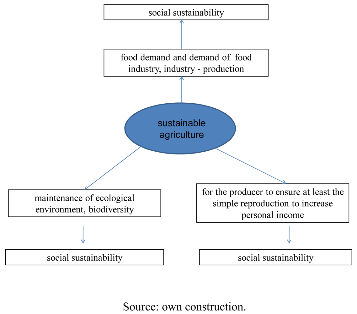
Social sustainability includes the necessary food production, industrial based energy production, also from the farmer's point of view, compliance with the profitability criteria, and the responsibility of sustaining the environment. The increase of world population, the carrying capacity of land and limited natural resources places agricultural production into a complex perspective, which necessitates the economic analysis of the role of intensive plant production technologies.</p>
<p>It should be emphasized that both ecological and social sustainability can only be realized if economic sustainability is reached during farming, and also on every level of human needs (<xref ref-type="fig" rid="f1-sustainability-03-01114">Figure 1</xref>).</p>
<p>The development of sustainability imposes special requirements on agriculture. Such varieties should be produced with technologies that allow the utilization of different, unique land qualities at reasonable costs, but, in the meantime, these should prohibit overloading the environment, and protect and preserve the biodiversity of the environment and basic resources. At the same time, the produced food and industrial goods should meet the needs of a growing population, especially in the matter of alternative, renewable energy sources.</p>
<p>From an economical and social sustainability point of view, amongst the agricultural resources, the conservation, reduce degradation or improvement of the growing soil and the water quality has the highest impact, and therefore in our opinion all trends and technologies should play a role/ be considered that allow the rational use of agrochemicals and therefore decrease the environmental impact at a given production level; also, at the same time, it can secure income for the agricultural workers and allow the optimal conditions for renewed reproduction.</p>
<p>In sustainable agriculture and rural development, the security of natural resources, and the security of food appear together by presuming and reinforcing each other. Our job is to find a degree of intensity matched with a form of farming technology that is appropriate for the environment. This farming framework alternative can create opportunities and allow different type of farming practices— such as organic, conventional, integrated and precision (a further developed form of integrated)—to be implemented even side by side.</p>
<p>Obviously, farm production cannot be separated from market movements, which also include the agricultural subsidies, their direction, and the degree with respect to the market demand [<xref ref-type="bibr" rid="b7-sustainability-03-01114">7</xref>–<xref ref-type="bibr" rid="b9-sustainability-03-01114">9</xref>]. Requirements stand against agricultural practices consequently yielding a restructuring pressure. The response to this pressure should be such as to allow economical usage of natural resources and currently available knowledge and experience. It means, in crop production, growers shall use the newest technologies along with different intensity production methods. In conjunction with the previously mentioned authors' view, in applying precision plant production, primarily pesticide use, could achieve a significant substance reduction, <italic>i.e.</italic>, a reduction of a real environmental load. It is important to emphasize, that the yield uncertainty by reducing the role of pesticides, contributes to the harvesting of a predictable yield, accomplishing one expectation for agriculture [<xref ref-type="bibr" rid="b10-sustainability-03-01114">10</xref>].</p></sec>
<sec>
<label>1.2.</label>
<title>The Role of Precision Pesticide Management in Precision Plant Production</title>
<p>Precision farming represents such a new farming strategy in crop production which would allow the farmer to implement a technology, adapted to the specific needs of the farm area with specific emphasis on chemical use. This may ensure a more efficient production for the grower along with a lower environmental impact. According to Wolf and Buttel [<xref ref-type="bibr" rid="b11-sustainability-03-01114">11</xref>], precision farming is an abiotic factor, which is the ultimate tool for the agricultural production's reform. Precision farming could allow the reduction of the chemical amount distributed in the environment by agricultural production, and it also could be one of the basic pillars of efficient agriculture, while allowing the large-scale production structure, investments, organizational structures and operational mechanisms to remain. Also, at the production level, this farming method can be a tool for reducing production risk. With the appropriate implementation and combination of technological elements in crop production, the uncertainty of yield can be reduced and the safety of a farmer's income can be increased [<xref ref-type="bibr" rid="b12-sustainability-03-01114">12</xref>–<xref ref-type="bibr" rid="b14-sustainability-03-01114">14</xref>]. This, however, requires the development and maintenance of technical background (additional investments) which means extra costs, which cannot always be recuperated in sales.</p>
<p>Precision fertilizing has already proved its cost efficiency. The bigger the farm, the more favorable and less risky the technology is [<xref ref-type="bibr" rid="b15-sustainability-03-01114">15</xref>,<xref ref-type="bibr" rid="b16-sustainability-03-01114">16</xref>]. Biermacher <italic>et al.</italic> [<xref ref-type="bibr" rid="b17-sustainability-03-01114">17</xref>] examined the economic suitability of precision nitrogen top dressing in winter wheat, by the nutrient supply online optical reflectance measurement. They have stated that in Oklahoma (USA) conditions this new technology is economically competitive against total-surface stock treatments [<xref ref-type="bibr" rid="b17-sustainability-03-01114">17</xref>]. Other authors claim that due to site-specific nutrient management technology, a higher yield can be harvested [<xref ref-type="bibr" rid="b18-sustainability-03-01114">18</xref>]. The cost-reducing impact and influencing factors of precision crop protection have been less analyzed by researchers. The economic advantage of introducing site specific crop protection, depends on the proportion of those crops that the process can be applied to in a technological sense, and whether the occurrence of damaging organs is changeable and if the proportion of infected area is low [<xref ref-type="bibr" rid="b19-sustainability-03-01114">19</xref>]. The given crop culture is determined from the aspect of its applicability for precision weed control. The economic interrelations require a multidisciplinary approach to the subject. The economic principle of weed control is simple: plant protection shall only be applied if the expected advantages (extra income) exceed its cost. The practical implementation of the damage-threshold principle requires the development of decision-support models, with which the experts also receive a tool for risk reduction. However, detailed knowledge of weed population and its development dynamics are often absent. Rider <italic>et al.</italic> [<xref ref-type="bibr" rid="b20-sustainability-03-01114">20</xref>] examined the extra income of location specific post-emergent weed control for each grid cell in the state of Kansas (USA). They mapped the weed population three weeks after treatment and modeled the impact of weed coverage on yield at the cell level. They stated that the post-emergent weed treatment had a traceable impact on the yield, but it could not be regarded as significant. The extra income covered only part of the cost of the precision treatment's cost, and therefore they could not justify the economical viability of the precision weed control <italic>versus</italic> the full surface weed treatment [<xref ref-type="bibr" rid="b20-sustainability-03-01114">20</xref>].</p>
<p>Simulation is a suitable tool for measuring the potential economic and environmental advantages of precision weed control. By modeling the economic consequences of site specific weed control in regard to weed coverage (such as the number of occurring weed varieties, specific density compared to the damage threshold, and weed vegetation phase at the given time), those relations can be revealed which determine whether positive results can be reached in an economic sense, and reveal what the main influencing factors are [<xref ref-type="bibr" rid="b21-sustainability-03-01114">21</xref>,<xref ref-type="bibr" rid="b22-sustainability-03-01114">22</xref>].</p>
<p>The above starting point shows that it is necessary to find the methods of analysis which will make it possible to evaluate the economic effects of risk reduction concerning crop protection chemical use at the farm level, sector level and national economy level. Among the investigated questions, priority shall be given to the examination of the impacts of different chemical risk reducing strategies to the farm income, agricultural employment, agricultural trade, GDP, and externalities (with special regard to water quality, biodiversity and human health).</p>
<p>In the second half of the last century, with the development of computer technology, several mathematical and operation research methods had been implemented in practice for modeling of economic decisions connected to crop protection, including weed management. Stochastic simulation—the Monte-Carlo method—was used for modeling the random effects in weed management, which can be rather significant during crop production. By exploring the degree of risk, this can offer more precise alternatives for decision making than the deterministic analyses.</p>
<p>During modeling agro-ecosystems, precision crop production is one of those areas where it is very important to assess the risk elements of crop production, such as weather, plant health, risk of production and market demand. With regard to precision weed management, the heterogeneity within the plot is of key importance. The biodynamic models are suitable for the examination of changes in agricultural systems (production structure, long-term economic impacts, and risks) during an extended period of time [<xref ref-type="bibr" rid="b23-sustainability-03-01114">23</xref>,<xref ref-type="bibr" rid="b24-sustainability-03-01114">24</xref>].</p>
<p>The objective of this current paper is to examine the economic relations and the consequences of precision weed control, as well as the risks of precision crop production.</p></sec></sec>
<sec sec-type="results|discussion">
<label>2.</label>
<title>Results and Discussion</title>
<p>
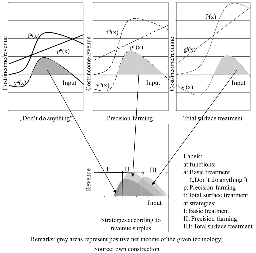
The concept of model analysis, based on the fact that different production technologies and methods result in different input-output relation systems, and therefore different production graphs (yield-, and cost curves) is described (<xref ref-type="fig" rid="f2-sustainability-03-01114">Figure 2</xref>) [<xref ref-type="bibr" rid="b25-sustainability-03-01114">25</xref>].</p>
<p>Several independent variables can impact yield, but only some of these are under the producer's control. In former researches, it has been proved that the effects of certain variables can be described by independent partial functions (<italic>i.e.</italic>, production function). According to this, it can be generally presumed that the subject can be examined with the production function. The following types of production functions were used in this study: nutrition–yield; weed coverage–yield.</p>
<p>The production function (output) depends on the production inputs:
<list list-type="bullet">
<list-item>
<p>Soil nutrient supply (<italic>x<sub>1</sub></italic>);</p></list-item>
<list-item>
<p>Fertilizer use (<italic>x</italic><sub>2</sub>);</p></list-item>
<list-item>
<p>Nutrient utilization graph of crop variety (<italic>x<sub>3</sub></italic>);</p></list-item>
<list-item>
<p>Weed coverage on the plot (<italic>x<sub>4</sub></italic>);</p></list-item>
<list-item>
<p>Method of weed treatment (weed control) (<italic>x<sub>5</sub></italic>);</p></list-item>
<list-item>
<p>Yield reducing impact of weeds on the plot (<italic>x<sub>6</sub></italic>).</p></list-item></list></p>
<disp-formula id="FD1">
<label>(1)</label>
<mml:math id="mm1" display="block">
<mml:semantics id="sm1">
<mml:mrow>
<mml:mi>X</mml:mi>
<mml:mo>=</mml:mo>
<mml:mi>f</mml:mi>
<mml:mo stretchy="false">(</mml:mo>
<mml:msub>
<mml:mi>x</mml:mi>
<mml:mi>k</mml:mi></mml:msub>
<mml:mo stretchy="false">)</mml:mo></mml:mrow></mml:semantics></mml:math></disp-formula>
<p>Variable costs of production 
<inline-formula>
<mml:math id="mm2" display="inline">
<mml:semantics id="sm2">
<mml:mrow>
<mml:mo stretchy="false">(</mml:mo>
<mml:msubsup>
<mml:mi>Z</mml:mi>
<mml:mi>i</mml:mi>
<mml:mi>c</mml:mi></mml:msubsup>
<mml:mo stretchy="false">)</mml:mo></mml:mrow></mml:semantics></mml:math></inline-formula>:
<list list-type="bullet">
<list-item>
<p>Input dependent variable costs
<list list-type="simple">
<list-item>
<label>□</label>
<p>Cost of fertilizer</p></list-item>
<list-item>
<label>□</label>
<p>Cost of chemicals used in weed management</p></list-item></list></p></list-item>
<list-item>
<p>Target yield dependent variable costs
<list list-type="simple">
<list-item>
<label>□</label>
<p>Sowing seed cost</p></list-item></list></p></list-item>
<list-item>
<p>Technology dependent costs
<list list-type="simple">
<list-item>
<label>□</label>
<p>Technological costs of fertilizer spreading</p></list-item>
<list-item>
<label>□</label>
<p>Technological costs of spreading of weed management chemicals</p></list-item></list></p></list-item>
<list-item>
<p>Costs dependent on realized yield
<list list-type="simple">
<list-item>
<label>□</label>
<p>Costs of drying</p></list-item>
<list-item>
<label>□</label>
<p>Cost of shipping</p></list-item></list></p></list-item>
<list-item>
<p>Area dependent costs
<list list-type="simple">
<list-item>
<label>□</label>
<p>Costs of harvesting</p></list-item></list></p></list-item></list></p>
<p>Constant cost factors of production 
<inline-formula>
<mml:math id="mm3" display="inline">
<mml:semantics id="sm3">
<mml:mrow>
<mml:mo stretchy="false">(</mml:mo>
<mml:msubsup>
<mml:mi>Z</mml:mi>
<mml:mi>j</mml:mi>
<mml:mi>c</mml:mi></mml:msubsup>
<mml:mo stretchy="false">)</mml:mo></mml:mrow></mml:semantics></mml:math></inline-formula>:
<list list-type="bullet">
<list-item>
<p>Technology dependent constant costs
<list list-type="simple">
<list-item>
<label>□</label>
<p>Amortization of technological means</p></list-item>
<list-item>
<label>□</label>
<p>External services assisting/enabling technological implementation</p></list-item></list></p></list-item>
<list-item>
<p>Constant costs connected to operation
<list list-type="simple">
<list-item>
<label>□</label>
<p>Wage costs</p>
<p>General costs of the farm connected to the production (professional extension service, soil analysis, <italic>etc.</italic>)</p></list-item></list></p></list-item></list></p>
<disp-formula id="FD2">
<label>(2)</label>
<mml:math id="mm4" display="block">
<mml:semantics id="sm4">
<mml:mrow>
<mml:mi>Z</mml:mi>
<mml:mo>=</mml:mo>
<mml:mi>f</mml:mi>
<mml:mrow>
<mml:mo>(</mml:mo>
<mml:mrow>
<mml:msubsup>
<mml:mi>z</mml:mi>
<mml:mi>i</mml:mi>
<mml:mi>c</mml:mi></mml:msubsup>
<mml:mo>,</mml:mo>
<mml:msubsup>
<mml:mi>z</mml:mi>
<mml:mi>j</mml:mi>
<mml:mi>v</mml:mi></mml:msubsup></mml:mrow>
<mml:mo>)</mml:mo></mml:mrow></mml:mrow></mml:semantics></mml:math></disp-formula>
<p>The profit depends on the yield and the costs.</p>
<disp-formula id="FD3">
<label>(3)</label>
<mml:math id="mm5" display="block">
<mml:semantics id="sm5">
<mml:mrow>
<mml:mi>N</mml:mi>
<mml:mo>=</mml:mo>
<mml:mi>f</mml:mi>
<mml:mo stretchy="false">(</mml:mo>
<mml:msub>
<mml:mi>x</mml:mi>
<mml:mi>k</mml:mi></mml:msub>
<mml:mo stretchy="false">)</mml:mo>
<mml:mo>−</mml:mo>
<mml:mo stretchy="false">(</mml:mo>
<mml:msubsup>
<mml:mi>z</mml:mi>
<mml:mi>i</mml:mi>
<mml:mi>c</mml:mi></mml:msubsup>
<mml:mo>,</mml:mo>
<mml:msubsup>
<mml:mi>z</mml:mi>
<mml:mi>j</mml:mi>
<mml:mi>c</mml:mi></mml:msubsup>
<mml:mo stretchy="false">)</mml:mo></mml:mrow></mml:semantics></mml:math></disp-formula>
<p>General form of income function (f(x)):
<disp-formula id="FD4">
<label>(4)</label>
<mml:math id="mm6" display="block">
<mml:semantics id="sm6">
<mml:mrow>
<mml:mi>f</mml:mi>
<mml:mo stretchy="false">(</mml:mo>
<mml:mi>x</mml:mi>
<mml:mo stretchy="false">)</mml:mo>
<mml:mo>=</mml:mo>
<mml:mfrac>
<mml:mi>A</mml:mi>
<mml:mrow>
<mml:mi>a</mml:mi>
<mml:mo>+</mml:mo>
<mml:msup>
<mml:mi>e</mml:mi>
<mml:mrow>
<mml:mi>b</mml:mi>
<mml:mo>⋅</mml:mo>
<mml:mi>x</mml:mi></mml:mrow></mml:msup></mml:mrow></mml:mfrac>
<mml:mo>+</mml:mo>
<mml:mi>k</mml:mi>
<mml:mo>⋅</mml:mo>
<mml:msup>
<mml:mi>x</mml:mi>
<mml:mn>2</mml:mn></mml:msup>
<mml:mo>+</mml:mo>
<mml:mi>l</mml:mi>
<mml:mo>⋅</mml:mo>
<mml:mi>x</mml:mi>
<mml:mo>+</mml:mo>
<mml:mi>m</mml:mi></mml:mrow></mml:semantics></mml:math></disp-formula>where:
<list list-type="simple">
<list-item>
<p><italic>x</italic> = input: natural production material input (kg), or value expressing it (currency unit);</p></list-item>
<list-item>
<p><italic>A</italic> = yield maximum constant (currency unit);</p></list-item>
<list-item>
<p><italic>a</italic> = constant of logistic function element;</p></list-item>
<list-item>
<p><italic>e</italic> = 2,7184…;</p></list-item>
<list-item>
<p><italic>b</italic> = shape factor coefficient of logistic function element;</p></list-item>
<list-item>
<p><italic>k</italic> = coefficient of quadratic element (currency unit-1);</p></list-item>
<list-item>
<p><italic>l</italic> = coefficient of linear element;</p></list-item>
<list-item>
<p><italic>m</italic> = constant (currency unit).</p></list-item></list></p>
<p>The parameters of this general model depend on the crops. Each investigated crop's (wheat, corn, sunflower) production function has been provided for modeling, based on scientific sources. These parameters will be described later on. With the usage of this theoretical model we have identified the strategic decision criteria for the precision weed management.</p>
<p>It is true for the equation that:
<disp-formula id="FD5">
<label>(5)</label>
<mml:math id="mm7" display="block">
<mml:semantics id="sm7">
<mml:mrow>
<mml:mi>f</mml:mi>
<mml:mo stretchy="false">(</mml:mo>
<mml:mi>x</mml:mi>
<mml:mo>=</mml:mo>
<mml:mn>0</mml:mn>
<mml:mo stretchy="false">)</mml:mo>
<mml:mo>=</mml:mo>
<mml:mn>0</mml:mn></mml:mrow></mml:semantics></mml:math></disp-formula></p>
<p>General form of cost function (g(x)):
<disp-formula id="FD6">
<label>(6)</label>
<mml:math id="mm8" display="block">
<mml:semantics id="sm8">
<mml:mrow>
<mml:mi>g</mml:mi>
<mml:mo stretchy="false">(</mml:mo>
<mml:mi>x</mml:mi>
<mml:mo stretchy="false">)</mml:mo>
<mml:mo>=</mml:mo>
<mml:msub>
<mml:mi>G</mml:mi>
<mml:mn>0</mml:mn></mml:msub>
<mml:mo>+</mml:mo>
<mml:mi>c</mml:mi>
<mml:mo>⋅</mml:mo>
<mml:mi>x</mml:mi></mml:mrow></mml:semantics></mml:math></disp-formula>where:
<list list-type="simple">
<list-item>
<p><italic>x</italic> = input (currency unit);</p></list-item>
<list-item>
<p><italic>G<sub>0</sub></italic> = constant cost component (currency unit);</p></list-item>
<list-item>
<p><italic>c</italic> = variable cost coefficient (currency unit/currency unit).</p></list-item></list>
<disp-formula id="FD7">
<label>(7)</label>
<mml:math id="mm9" display="block">
<mml:semantics id="sm9">
<mml:mrow>
<mml:mi>c</mml:mi>
<mml:mo>=</mml:mo>
<mml:munderover>
<mml:mo>∑</mml:mo>
<mml:mrow>
<mml:mi>i</mml:mi>
<mml:mo>=</mml:mo>
<mml:mn>1</mml:mn></mml:mrow>
<mml:mi>n</mml:mi></mml:munderover>
<mml:mrow>
<mml:msub>
<mml:mi>c</mml:mi>
<mml:mi>i</mml:mi></mml:msub></mml:mrow></mml:mrow></mml:semantics></mml:math></disp-formula>where:
<list list-type="simple">
<list-item>
<p><italic>c<sub>i</sub></italic> = variable cost component of variable no. <italic>i</italic> (currency unit/currency unit);</p></list-item>
<list-item>
<p><italic>n</italic> = number of variable cost component varieties.</p></list-item></list></p>
<p>In the simulation model incorporated nutrient–yield and weed coverage–yield functions were determined based on previous experiments. This base was provided by the researchers of the Cereal Research Non-profit Limited Liability Corporation (Szeged, former Cereal Research Ltd.), the Agricultural Research Institute of the Hungarian Academy of Sciences (Martonvásár), and also contextures published by other weed researchers.</p>
<p>It is true for the interrelation that:
<disp-formula id="FD8">
<label>(8)</label>
<mml:math id="mm10" display="block">
<mml:semantics id="sm10">
<mml:mrow>
<mml:mi>g</mml:mi>
<mml:mo stretchy="false">(</mml:mo>
<mml:mi>x</mml:mi>
<mml:mo>=</mml:mo>
<mml:mn>0</mml:mn>
<mml:mo stretchy="false">)</mml:mo>
<mml:mo>=</mml:mo>
<mml:msub>
<mml:mi>G</mml:mi>
<mml:mn>0</mml:mn></mml:msub></mml:mrow></mml:semantics></mml:math></disp-formula></p>
<p>General form of revenue (net income) function:
<disp-formula id="FD9">
<label>(9)</label>
<mml:math id="mm11" display="block">
<mml:semantics id="sm11">
<mml:mrow>
<mml:mi>y</mml:mi>
<mml:mo stretchy="false">(</mml:mo>
<mml:mi>x</mml:mi>
<mml:mo stretchy="false">)</mml:mo>
<mml:mo>=</mml:mo>
<mml:mi>f</mml:mi>
<mml:mo stretchy="false">(</mml:mo>
<mml:mi>x</mml:mi>
<mml:mo stretchy="false">)</mml:mo>
<mml:mo>−</mml:mo>
<mml:mi>g</mml:mi>
<mml:mo stretchy="false">(</mml:mo>
<mml:mi>x</mml:mi>
<mml:mo stretchy="false">)</mml:mo></mml:mrow></mml:semantics></mml:math></disp-formula></p>
<p>Upper index indicates the graph types according to the following:
<list list-type="simple">
<list-item>
<p><italic>a</italic> = basic type treatment (“Don't do anything”);</p></list-item>
<list-item>
<p><italic>p</italic> = precision farming;</p></list-item>
<list-item>
<p><italic>t</italic> = total, undifferentiated surface treatment;</p></list-item></list></p>
<p>Ranges set up; for three weed management strategies, based on profitability:
<list list-type="roman-upper">
<list-item>
<p>Basic treatment: “Don't do anything”, (means: do not treat the area with herbicides)
<disp-formula id="FD10">
<label>(10)</label>
<mml:math id="mm12" display="block">
<mml:semantics id="sm12">
<mml:mrow>
<mml:msup>
<mml:mi>y</mml:mi>
<mml:mi>a</mml:mi></mml:msup>
<mml:mo stretchy="false">(</mml:mo>
<mml:mi>x</mml:mi>
<mml:mo stretchy="false">)</mml:mo>
<mml:mo>≥</mml:mo>
<mml:msup>
<mml:mi>y</mml:mi>
<mml:mi>p</mml:mi></mml:msup>
<mml:mo stretchy="false">(</mml:mo>
<mml:mi>x</mml:mi>
<mml:mo stretchy="false">)</mml:mo>
<mml:mspace width="0.2em"/>
<mml:mtext mathvariant="italic">and</mml:mtext>
<mml:mspace width="0.2em"/>
<mml:msup>
<mml:mi>y</mml:mi>
<mml:mi>t</mml:mi></mml:msup>
<mml:mo stretchy="false">(</mml:mo>
<mml:mi>x</mml:mi>
<mml:mo stretchy="false">)</mml:mo></mml:mrow></mml:semantics></mml:math></disp-formula>Its limit is the damage threshold:
<disp-formula id="FD11">
<label>(11)</label>
<mml:math id="mm13" display="block">
<mml:semantics id="sm13">
<mml:mrow>
<mml:msup>
<mml:mi>y</mml:mi>
<mml:mi>a</mml:mi></mml:msup>
<mml:mo stretchy="false">(</mml:mo>
<mml:mi>x</mml:mi>
<mml:mo stretchy="false">)</mml:mo>
<mml:mo>=</mml:mo>
<mml:msup>
<mml:mi>y</mml:mi>
<mml:mi>p</mml:mi></mml:msup>
<mml:mo stretchy="false">(</mml:mo>
<mml:mi>x</mml:mi>
<mml:mo stretchy="false">)</mml:mo>
<mml:mspace width="0.2em"/>
<mml:mtext mathvariant="italic">or</mml:mtext>
<mml:mspace width="0.2em"/>
<mml:msup>
<mml:mi>y</mml:mi>
<mml:mi>t</mml:mi></mml:msup>
<mml:mo stretchy="false">(</mml:mo>
<mml:mi>x</mml:mi>
<mml:mo stretchy="false">)</mml:mo></mml:mrow></mml:semantics></mml:math></disp-formula></p></list-item>
<list-item>
<p>Range of implementing precision technology
<disp-formula id="FD12">
<label>(12)</label>
<mml:math id="mm14" display="block">
<mml:semantics id="sm14">
<mml:mrow>
<mml:msup>
<mml:mi>y</mml:mi>
<mml:mi>a</mml:mi></mml:msup>
<mml:mo stretchy="false">(</mml:mo>
<mml:mi>x</mml:mi>
<mml:mo stretchy="false">)</mml:mo>
<mml:mo>&lt;</mml:mo>
<mml:msup>
<mml:mi>y</mml:mi>
<mml:mi>p</mml:mi></mml:msup>
<mml:mo stretchy="false">(</mml:mo>
<mml:mi>x</mml:mi>
<mml:mo stretchy="false">)</mml:mo>
<mml:mo>≥</mml:mo>
<mml:msup>
<mml:mi>y</mml:mi>
<mml:mi>t</mml:mi></mml:msup>
<mml:mo stretchy="false">(</mml:mo>
<mml:mi>x</mml:mi>
<mml:mo stretchy="false">)</mml:mo></mml:mrow></mml:semantics></mml:math></disp-formula></p></list-item>
<list-item>
<p>Application range of full-surface, undifferentiated treatment
<disp-formula id="FD13">
<label>(13)</label>
<mml:math id="mm15" display="block">
<mml:semantics id="sm15">
<mml:mrow>
<mml:msup>
<mml:mi>y</mml:mi>
<mml:mi>a</mml:mi></mml:msup>
<mml:mo stretchy="false">(</mml:mo>
<mml:mi>x</mml:mi>
<mml:mo stretchy="false">)</mml:mo>
<mml:mspace width="0.2em"/>
<mml:mtext mathvariant="italic">or</mml:mtext>
<mml:mspace width="0.2em"/>
<mml:msup>
<mml:mi>y</mml:mi>
<mml:mi>p</mml:mi></mml:msup>
<mml:mo stretchy="false">(</mml:mo>
<mml:mi>x</mml:mi>
<mml:mo stretchy="false">)</mml:mo>
<mml:mo>&lt;</mml:mo>
<mml:msup>
<mml:mi>y</mml:mi>
<mml:mi>t</mml:mi></mml:msup>
<mml:mo stretchy="false">(</mml:mo>
<mml:mi>x</mml:mi>
<mml:mo stretchy="false">)</mml:mo></mml:mrow></mml:semantics></mml:math></disp-formula></p></list-item></list></p>
<p>Besides the previously introduced production functions, each section of the production function can be described with partial equations. During modeling we have used the expense–yield functions, based on the previously mentioned research station's data. These are as follows.</p>
<p>Yield realized per unit area
<disp-formula id="FD14">
<label>(14)</label>
<mml:math id="mm16" display="block">
<mml:semantics id="sm16">
<mml:mrow>
<mml:msub>
<mml:mi>I</mml:mi>
<mml:mi>i</mml:mi></mml:msub>
<mml:mo>=</mml:mo>
<mml:mrow>
<mml:mo>(</mml:mo>
<mml:mrow>
<mml:mi>α</mml:mi>
<mml:mo>⋅</mml:mo>
<mml:msubsup>
<mml:mi>x</mml:mi>
<mml:mi>i</mml:mi>
<mml:mn>2</mml:mn></mml:msubsup>
<mml:mo>+</mml:mo>
<mml:mi>β</mml:mi>
<mml:mo>⋅</mml:mo>
<mml:msub>
<mml:mi>x</mml:mi>
<mml:mi>i</mml:mi></mml:msub>
<mml:mo>+</mml:mo>
<mml:mi>γ</mml:mi></mml:mrow>
<mml:mo>)</mml:mo></mml:mrow>
<mml:mo>⋅</mml:mo>
<mml:msub>
<mml:mrow>
<mml:mrow>
<mml:mo>(</mml:mo>
<mml:mrow>
<mml:mi>κ</mml:mi>
<mml:mo>⋅</mml:mo>
<mml:msubsup>
<mml:mi>w</mml:mi>
<mml:mi>i</mml:mi>
<mml:mn>2</mml:mn></mml:msubsup>
<mml:mo>+</mml:mo>
<mml:mi>λ</mml:mi>
<mml:mo>⋅</mml:mo>
<mml:msub>
<mml:mi>w</mml:mi>
<mml:mi>i</mml:mi></mml:msub>
<mml:mo>+</mml:mo>
<mml:mi>μ</mml:mi></mml:mrow>
<mml:mo>)</mml:mo></mml:mrow></mml:mrow>
<mml:mi>i</mml:mi></mml:msub></mml:mrow></mml:semantics></mml:math></disp-formula></p>
<p>Income / production value, realized per unit area
<disp-formula id="FD15">
<label>(15)</label>
<mml:math id="mm17" display="block">
<mml:semantics id="sm17">
<mml:mrow>
<mml:mi>I</mml:mi>
<mml:mo>=</mml:mo>
<mml:mi>p</mml:mi>
<mml:mo>⋅</mml:mo>
<mml:munderover>
<mml:mo>∑</mml:mo>
<mml:mrow>
<mml:mi>i</mml:mi>
<mml:mo>=</mml:mo>
<mml:mn>1</mml:mn></mml:mrow>
<mml:mi>n</mml:mi></mml:munderover>
<mml:mrow>
<mml:mrow>
<mml:mo>(</mml:mo>
<mml:mrow>
<mml:msub>
<mml:mi>I</mml:mi>
<mml:mi>i</mml:mi></mml:msub>
<mml:mo>⋅</mml:mo>
<mml:msub>
<mml:mi>T</mml:mi>
<mml:mi>i</mml:mi></mml:msub></mml:mrow>
<mml:mo>)</mml:mo></mml:mrow></mml:mrow></mml:mrow></mml:semantics></mml:math></disp-formula></p>
<p>In this case:
<list list-type="simple">
<list-item>
<p><italic>I</italic> = revenue realized per unit area (currency unit);</p></list-item>
<list-item>
<p><italic>I<sub>i</sub></italic> = yield realized in <italic>i</italic> cell (t/cell);</p></list-item>
<list-item>
<p><italic>p</italic> = sales unit price (currency unit/t);</p></list-item>
<list-item>
<p><italic>n</italic> = number of cell per field (pcs of cell);</p></list-item>
<list-item>
<p><italic>x<sub>i</sub></italic> = nutrient level of <italic>i</italic> cell, after nutrient application, data presented in nitrogen active ingredient (kg/ha).</p></list-item></list>
<disp-formula id="FD16">
<label>(16)</label>
<mml:math id="mm18" display="block">
<mml:semantics id="sm18">
<mml:mrow>
<mml:msub>
<mml:mi>x</mml:mi>
<mml:mi>i</mml:mi></mml:msub>
<mml:mo>=</mml:mo>
<mml:msubsup>
<mml:mi>x</mml:mi>
<mml:mi>i</mml:mi>
<mml:mn>0</mml:mn></mml:msubsup>
<mml:mo>+</mml:mo>
<mml:msubsup>
<mml:mi>x</mml:mi>
<mml:mi>i</mml:mi>
<mml:mi>a</mml:mi></mml:msubsup></mml:mrow></mml:semantics></mml:math></disp-formula>where:
<list list-type="simple">
<list-item>
<p><italic>x<sup>0</sup><sub>i</sub></italic> = the soil nutrient availability, shown in nitrogen active ingredient (kg/ha);</p></list-item>
<list-item>
<p><italic>x<sup>a</sup><sub>i</sub></italic> = nitrogen (active ingredient) applied to <italic>i</italic> cell (kg/ha);</p></list-item>
<list-item>
<p><italic>α</italic> = quadratic parameter of the yield function (t/kg<sup>2</sup>);</p></list-item>
<list-item>
<p><italic>β</italic> = first instance of the yield function (t/kg);</p></list-item>
<list-item>
<p><italic>γ</italic> = constant of the yield function (t/ha);</p></list-item>
<list-item>
<p><italic>w<sub>i</sub></italic> = weed coverage of <italic>i</italic> cell (%);</p></list-item>
<list-item>
<p><italic>κ</italic> = second degree parameter of the weed coverage yield influencing factor (t/ha/%<sup>2</sup>);</p></list-item>
<list-item>
<p><italic>λ</italic> = first degree parameter of the weed coverage yield influencing factor (t/ha/%);</p></list-item>
<list-item>
<p><italic>μ</italic> = constant parameter of the weed coverage yield influencing factor (t/ha), at original set <italic>μ</italic> = 0;</p></list-item>
<list-item>
<p><italic>T<sub>i</sub></italic> = <italic>i</italic> cell's area (ha/cell).</p></list-item></list></p>
<p><xref ref-type="table" rid="t1-sustainability-03-01114">Table 1</xref> shows a summary of the parameters of the functions.</p>
<p>During calculation of production costs, the possible differentiation driven from the different cell size should be taken into account, separated by the size dependent and yield dependant cost factors.</p>
<p>Unit area's production costs:
<disp-formula id="FD17">
<label>(17)</label>
<mml:math id="mm19" display="block">
<mml:semantics id="sm19">
<mml:mrow>
<mml:mtext>C</mml:mtext>
<mml:mo stretchy="false">(</mml:mo>
<mml:mtext>x</mml:mtext>
<mml:mo stretchy="false">(</mml:mo>
<mml:mi>ξ</mml:mi>
<mml:mo stretchy="false">)</mml:mo>
<mml:mo>,</mml:mo>
<mml:mtext>w</mml:mtext>
<mml:mo stretchy="false">(</mml:mo>
<mml:mi>ξ</mml:mi>
<mml:mo stretchy="false">)</mml:mo>
<mml:mo>=</mml:mo>
<mml:munderover>
<mml:mo>∑</mml:mo>
<mml:mrow>
<mml:mtext>i</mml:mtext>
<mml:mo>=</mml:mo>
<mml:mn>1</mml:mn></mml:mrow>
<mml:mtext>n</mml:mtext></mml:munderover>
<mml:mrow>
<mml:mrow>
<mml:mo>(</mml:mo>
<mml:mrow>
<mml:munderover>
<mml:mo>∑</mml:mo>
<mml:mrow>
<mml:mtext>j</mml:mtext>
<mml:mo>=</mml:mo>
<mml:mn>1</mml:mn></mml:mrow>
<mml:mtext>m</mml:mtext></mml:munderover>
<mml:mrow>
<mml:msub>
<mml:mtext>T</mml:mtext>
<mml:mtext>i</mml:mtext></mml:msub>
<mml:mo>⋅</mml:mo>
<mml:msubsup>
<mml:mtext>c</mml:mtext>
<mml:mtext>k</mml:mtext>
<mml:mrow>
<mml:mtext>vT</mml:mtext></mml:mrow></mml:msubsup>
<mml:mo>+</mml:mo>
<mml:munderover>
<mml:mo>∑</mml:mo>
<mml:mrow>
<mml:mtext>k</mml:mtext>
<mml:mo>=</mml:mo>
<mml:mn>1</mml:mn></mml:mrow>
<mml:mtext>o</mml:mtext></mml:munderover>
<mml:mrow>
<mml:msub>
<mml:mtext>T</mml:mtext>
<mml:mtext>i</mml:mtext></mml:msub>
<mml:mo>⋅</mml:mo>
<mml:msub>
<mml:mtext>I</mml:mtext>
<mml:mtext>i</mml:mtext></mml:msub>
<mml:mo>⋅</mml:mo>
<mml:msubsup>
<mml:mtext>c</mml:mtext>
<mml:mtext>k</mml:mtext>
<mml:mrow>
<mml:mtext>vI</mml:mtext></mml:mrow></mml:msubsup>
<mml:mo>+</mml:mo>
<mml:msub>
<mml:mi>ρ</mml:mi>
<mml:mtext>f</mml:mtext></mml:msub>
<mml:mo>⋅</mml:mo>
<mml:msubsup>
<mml:mtext>c</mml:mtext>
<mml:mtext>k</mml:mtext>
<mml:mrow>
<mml:mtext>vI</mml:mtext></mml:mrow></mml:msubsup>
<mml:mrow>
<mml:mo>(</mml:mo>
<mml:mrow>
<mml:msub>
<mml:mtext>x</mml:mtext>
<mml:mtext>i</mml:mtext></mml:msub>
<mml:mrow>
<mml:mo>〈</mml:mo>
<mml:mrow>
<mml:msubsup>
<mml:mtext>x</mml:mtext>
<mml:mtext>i</mml:mtext>
<mml:mn>0</mml:mn></mml:msubsup>
<mml:mo>,</mml:mo>
<mml:mrow>
<mml:mo>[</mml:mo>
<mml:mrow>
<mml:msub>
<mml:mtext>x</mml:mtext>
<mml:mrow>
<mml:mtext>min</mml:mtext></mml:mrow></mml:msub>
<mml:mo>,</mml:mo>
<mml:msub>
<mml:mtext>x</mml:mtext>
<mml:mrow>
<mml:mtext>max</mml:mtext></mml:mrow></mml:msub></mml:mrow>
<mml:mo>]</mml:mo></mml:mrow>
<mml:mo>,</mml:mo>
<mml:mi>ξ</mml:mi></mml:mrow>
<mml:mo>〉</mml:mo></mml:mrow></mml:mrow>
<mml:mo>)</mml:mo></mml:mrow>
<mml:mo>+</mml:mo>
<mml:msub>
<mml:mi>ρ</mml:mi>
<mml:mtext>w</mml:mtext></mml:msub>
<mml:mo>⋅</mml:mo>
<mml:msubsup>
<mml:mtext>c</mml:mtext>
<mml:mtext>w</mml:mtext>
<mml:mrow>
<mml:mtext>vI</mml:mtext></mml:mrow></mml:msubsup>
<mml:mrow>
<mml:mo>(</mml:mo>
<mml:mrow>
<mml:msub>
<mml:mtext>w</mml:mtext>
<mml:mtext>i</mml:mtext></mml:msub>
<mml:mrow>
<mml:mo>〈</mml:mo>
<mml:mrow>
<mml:mrow>
<mml:mo>[</mml:mo>
<mml:mrow>
<mml:msub>
<mml:mtext>w</mml:mtext>
<mml:mrow>
<mml:mtext>min</mml:mtext></mml:mrow></mml:msub>
<mml:mo>,</mml:mo>
<mml:msub>
<mml:mtext>w</mml:mtext>
<mml:mrow>
<mml:mtext>max</mml:mtext></mml:mrow></mml:msub></mml:mrow>
<mml:mo>]</mml:mo></mml:mrow>
<mml:mo>,</mml:mo>
<mml:mi>ξ</mml:mi></mml:mrow>
<mml:mo>〉</mml:mo></mml:mrow></mml:mrow>
<mml:mo>)</mml:mo></mml:mrow></mml:mrow></mml:mrow></mml:mrow>
<mml:mo>)</mml:mo></mml:mrow></mml:mrow>
<mml:mo>+</mml:mo>
<mml:msup>
<mml:mtext>C</mml:mtext>
<mml:mn>0</mml:mn></mml:msup></mml:mrow></mml:semantics></mml:math></disp-formula>where:
<list list-type="simple">
<list-item>
<p><italic>n</italic> = number of cell (pcs));</p></list-item>
<list-item>
<p><italic>m</italic> = number of area dependant cost items (pcs);</p></list-item>
<list-item>
<p><italic>o</italic> = number of yield dependent cost items (pcs);</p></list-item>
<list-item>
<p><italic>T<sub>i</sub></italic> = size of <italic>i</italic> cell (ha/cell);</p></list-item>
<list-item>
<p><italic>I<sub>i</sub></italic> = average yield of <italic>i</italic> cell (t/ha);</p></list-item>
<list-item>
<p><italic>c<sup>vT</sup><sub>1</sub></italic> = seed cost (currency unit/ha);</p></list-item>
<list-item>
<p><italic>c<sup>vT</sup><sub>2</sub></italic> = variable equipment cost (currency unit/ha);</p></list-item>
<list-item>
<p><italic>c<sup>vT</sup><sub>3</sub></italic> = variable cost of paid machinery work depending on cultivating area (currency unit/ha);</p></list-item>
<list-item>
<p><italic>c<sup>vI</sup><sub>1</sub></italic> = cost of drying (currency unit/ha);</p></list-item>
<list-item>
<p><italic>c<sup>vI</sup><sub>2</sub></italic> = variable cost of transport and post harvest activities (currency unit/t);</p></list-item>
<list-item>
<p><italic>C<sup>0</sup></italic> = technological split constant cost (currency unit/ha).</p></list-item></list></p>
<disp-formula id="FD18">
<label>(18)</label>
<mml:math id="mm20" display="block">
<mml:semantics id="sm20">
<mml:mrow>
<mml:msubsup>
<mml:mi>c</mml:mi>
<mml:mtext>i</mml:mtext>
<mml:mi>f</mml:mi></mml:msubsup>
<mml:mrow>
<mml:mo>(</mml:mo>
<mml:mrow>
<mml:msub>
<mml:mi>x</mml:mi>
<mml:mi>i</mml:mi></mml:msub>
<mml:mrow>
<mml:mo>(</mml:mo>
<mml:mi>ξ</mml:mi>
<mml:mo>)</mml:mo></mml:mrow></mml:mrow>
<mml:mo>)</mml:mo></mml:mrow>
<mml:mo>=</mml:mo>
<mml:msub>
<mml:mi>ρ</mml:mi>
<mml:mi>f</mml:mi></mml:msub>
<mml:mo>⋅</mml:mo>
<mml:msubsup>
<mml:mi>m</mml:mi>
<mml:mi>f</mml:mi>
<mml:mrow>
<mml:mi>v</mml:mi>
<mml:mi>I</mml:mi></mml:mrow></mml:msubsup>
<mml:mrow>
<mml:mo>(</mml:mo>
<mml:mrow>
<mml:msub>
<mml:mtext>x</mml:mtext>
<mml:mi>i</mml:mi></mml:msub>
<mml:mrow>
<mml:mo>〈</mml:mo>
<mml:mrow>
<mml:msubsup>
<mml:mtext>x</mml:mtext>
<mml:mi>i</mml:mi>
<mml:mn>0</mml:mn></mml:msubsup>
<mml:mo>,</mml:mo>
<mml:mrow>
<mml:mo>[</mml:mo>
<mml:mrow>
<mml:msub>
<mml:mtext>x</mml:mtext>
<mml:mrow>
<mml:mtext>min</mml:mtext></mml:mrow></mml:msub>
<mml:mo>,</mml:mo>
<mml:msub>
<mml:mi>x</mml:mi>
<mml:mrow>
<mml:mtext>max</mml:mtext></mml:mrow></mml:msub></mml:mrow>
<mml:mo>]</mml:mo></mml:mrow>
<mml:mo>,</mml:mo>
<mml:mi>ξ</mml:mi></mml:mrow>
<mml:mo>〉</mml:mo></mml:mrow></mml:mrow>
<mml:mo>)</mml:mo></mml:mrow>
<mml:mo>⋅</mml:mo>
<mml:msub>
<mml:mi>T</mml:mi>
<mml:mi>i</mml:mi></mml:msub></mml:mrow></mml:semantics></mml:math></disp-formula>
<disp-formula id="FD19">
<label>(19)</label>
<mml:math id="mm21" display="block">
<mml:semantics id="sm21">
<mml:mrow>
<mml:msubsup>
<mml:mi>c</mml:mi>
<mml:mtext>i</mml:mtext>
<mml:mtext>w</mml:mtext></mml:msubsup>
<mml:mrow>
<mml:mo>(</mml:mo>
<mml:mrow>
<mml:msub>
<mml:mtext>w</mml:mtext>
<mml:mi>i</mml:mi></mml:msub>
<mml:mrow>
<mml:mo>(</mml:mo>
<mml:mi>ξ</mml:mi>
<mml:mo>)</mml:mo></mml:mrow></mml:mrow>
<mml:mo>)</mml:mo></mml:mrow>
<mml:mo>=</mml:mo>
<mml:msub>
<mml:mi>ρ</mml:mi>
<mml:mtext>w</mml:mtext></mml:msub>
<mml:mo>⋅</mml:mo>
<mml:msubsup>
<mml:mi>m</mml:mi>
<mml:mi>w</mml:mi>
<mml:mrow>
<mml:mi>v</mml:mi>
<mml:mi>I</mml:mi></mml:mrow></mml:msubsup>
<mml:mrow>
<mml:mo>(</mml:mo>
<mml:mrow>
<mml:msub>
<mml:mi>w</mml:mi>
<mml:mi>i</mml:mi></mml:msub>
<mml:mrow>
<mml:mo>〈</mml:mo>
<mml:mrow>
<mml:mrow>
<mml:mo>[</mml:mo>
<mml:mrow>
<mml:msub>
<mml:mi>w</mml:mi>
<mml:mrow>
<mml:mtext>min</mml:mtext></mml:mrow></mml:msub>
<mml:mo>,</mml:mo>
<mml:msub>
<mml:mi>w</mml:mi>
<mml:mrow>
<mml:mtext>max</mml:mtext></mml:mrow></mml:msub></mml:mrow>
<mml:mo>]</mml:mo></mml:mrow>
<mml:mo>,</mml:mo>
<mml:mi>ξ</mml:mi></mml:mrow>
<mml:mo>〉</mml:mo></mml:mrow></mml:mrow>
<mml:mo>)</mml:mo></mml:mrow>
<mml:mo>⋅</mml:mo>
<mml:msub>
<mml:mi>T</mml:mi>
<mml:mi>i</mml:mi></mml:msub></mml:mrow></mml:semantics></mml:math></disp-formula>
<list list-type="simple">
<list-item>
<p><italic>c<sup>f</sup><sub>i</sub>(x<sub>i</sub>(ξ))</italic> = nutrition cost on cell level accordance to the applied nutrition (currency unit/ha);</p></list-item>
<list-item>
<p><italic>c<sup>w</sup><sub>i</sub>(w<sub>i</sub>(ξ))</italic> = cost of pesticide on cell level, according to the cell's weed coverage and the applied chemical amount (currency unit/cell);</p></list-item>
<list-item>
<p><italic>ρ<sub>f</sub></italic> = fertility unit price according to active ingredient (currency unit/kg);</p></list-item>
<list-item>
<p><italic>ρ<sub>w</sub></italic> = average chemical cost of elimination of 1% weed (currency unit/ha);</p></list-item>
<list-item>
<p>
<inline-formula>
<mml:math id="mm22" display="inline">
<mml:semantics id="sm22">
<mml:mrow>
<mml:msubsup>
<mml:mi>m</mml:mi>
<mml:mi>f</mml:mi>
<mml:mrow>
<mml:mi>v</mml:mi>
<mml:mi>I</mml:mi></mml:mrow></mml:msubsup>
<mml:mrow>
<mml:mo>(</mml:mo>
<mml:mrow>
<mml:msub>
<mml:mtext>x</mml:mtext>
<mml:mtext>i</mml:mtext></mml:msub>
<mml:mrow>
<mml:mo>〈</mml:mo>
<mml:mrow>
<mml:msubsup>
<mml:mtext>x</mml:mtext>
<mml:mtext>i</mml:mtext>
<mml:mn>0</mml:mn></mml:msubsup>
<mml:mo>,</mml:mo>
<mml:mrow>
<mml:mo>[</mml:mo>
<mml:mrow>
<mml:msub>
<mml:mtext>x</mml:mtext>
<mml:mrow>
<mml:mtext>min</mml:mtext></mml:mrow></mml:msub>
<mml:mo>,</mml:mo>
<mml:msub>
<mml:mtext>x</mml:mtext>
<mml:mrow>
<mml:mtext>max</mml:mtext></mml:mrow></mml:msub></mml:mrow>
<mml:mo>]</mml:mo></mml:mrow>
<mml:mo>,</mml:mo>
<mml:mi>ξ</mml:mi></mml:mrow>
<mml:mo>〉</mml:mo></mml:mrow></mml:mrow>
<mml:mo>)</mml:mo></mml:mrow></mml:mrow></mml:semantics></mml:math></inline-formula> = the <italic>i<sup>th</sup></italic> cell fertilizer dose per hectare, 
<inline-formula>
<mml:math id="mm23" display="inline">
<mml:semantics id="sm23">
<mml:mrow>
<mml:msubsup>
<mml:mi>x</mml:mi>
<mml:mi>i</mml:mi>
<mml:mn>0</mml:mn></mml:msubsup></mml:mrow></mml:semantics></mml:math></inline-formula> nutritional supply level, [x<sub>min</sub>, x<sub>max</sub>] nutritional input range; <italic>ξ</italic> in random value specified nutrient levels (kg/ha);</p></list-item>
<list-item>
<p>
<inline-formula>
<mml:math id="mm24" display="inline">
<mml:semantics id="sm24">
<mml:mrow>
<mml:msubsup>
<mml:mi>m</mml:mi>
<mml:mtext>w</mml:mtext>
<mml:mrow>
<mml:mi>v</mml:mi>
<mml:mi>I</mml:mi></mml:mrow></mml:msubsup>
<mml:mrow>
<mml:mo>(</mml:mo>
<mml:mrow>
<mml:msub>
<mml:mtext>w</mml:mtext>
<mml:mtext>i</mml:mtext></mml:msub>
<mml:mrow>
<mml:mo>〈</mml:mo>
<mml:mrow>
<mml:mrow>
<mml:mo>[</mml:mo>
<mml:mrow>
<mml:msub>
<mml:mtext>w</mml:mtext>
<mml:mrow>
<mml:mtext>min</mml:mtext></mml:mrow></mml:msub>
<mml:mo>,</mml:mo>
<mml:msub>
<mml:mi>w</mml:mi>
<mml:mrow>
<mml:mtext>max</mml:mtext></mml:mrow></mml:msub></mml:mrow>
<mml:mo>]</mml:mo></mml:mrow>
<mml:mo>,</mml:mo>
<mml:mi>ξ</mml:mi></mml:mrow>
<mml:mo>〉</mml:mo></mml:mrow></mml:mrow>
<mml:mo>)</mml:mo></mml:mrow></mml:mrow></mml:semantics></mml:math></inline-formula> = the <italic>i<sup>th</sup></italic> cell applied chemical dose per hectare in the application range [w<sub>min</sub>, w<sub>max</sub>] at <italic>ξ</italic> random nutritional level (kg/ha);</p></list-item>
<list-item>
<p><italic>ξ</italic> = standard deviation random number in range [0,1].</p></list-item></list>
<p><xref ref-type="table" rid="t2-sustainability-03-01114">Table 2</xref>. shows the base values used for the cost calculation.</p>
<p>
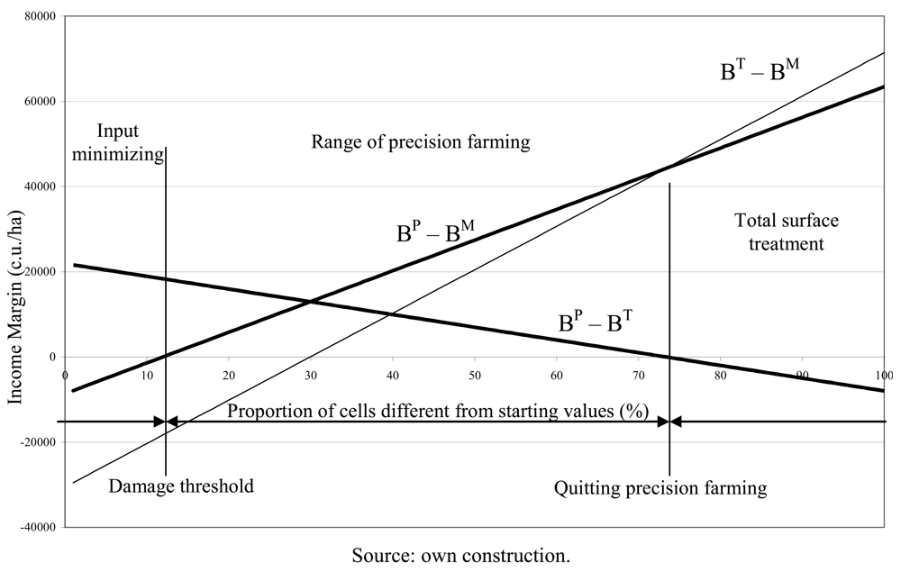
With the help of the yield and cost function, the profit function on cell level can be described. This profit function shows the marginal criteria of the application of the precision technique. This will allow the designation of the economical domain, such as threshold (entering and quitting threshold), and the ranges bordered by these. (<xref ref-type="fig" rid="f3-sustainability-03-01114">Figure 3</xref>).</p>
<p>The technological variety's profit function:
<disp-formula id="FD20">
<label>(20)</label>
<mml:math id="mm26" display="block">
<mml:semantics id="sm26">
<mml:mrow>
<mml:mi>B</mml:mi>
<mml:mo stretchy="false">(</mml:mo>
<mml:mi>x</mml:mi>
<mml:mo stretchy="false">(</mml:mo>
<mml:mi>ξ</mml:mi>
<mml:mo stretchy="false">)</mml:mo>
<mml:mo>,</mml:mo>
<mml:mi>w</mml:mi>
<mml:mo stretchy="false">(</mml:mo>
<mml:mi>ξ</mml:mi>
<mml:mo stretchy="false">)</mml:mo>
<mml:mo>,</mml:mo>
<mml:mi>φ</mml:mi>
<mml:mo stretchy="false">)</mml:mo>
<mml:mo>=</mml:mo>
<mml:mi>I</mml:mi>
<mml:mo stretchy="false">(</mml:mo>
<mml:mi>x</mml:mi>
<mml:mo stretchy="false">(</mml:mo>
<mml:mi>ξ</mml:mi>
<mml:mo stretchy="false">)</mml:mo>
<mml:mo>,</mml:mo>
<mml:mi>w</mml:mi>
<mml:mo stretchy="false">(</mml:mo>
<mml:mi>ξ</mml:mi>
<mml:mo stretchy="false">)</mml:mo>
<mml:mo>,</mml:mo>
<mml:mi>φ</mml:mi>
<mml:mo stretchy="false">)</mml:mo>
<mml:mo>−</mml:mo>
<mml:mi>C</mml:mi>
<mml:mo stretchy="false">(</mml:mo>
<mml:mi>x</mml:mi>
<mml:mo stretchy="false">(</mml:mo>
<mml:mi>ξ</mml:mi>
<mml:mo stretchy="false">)</mml:mo>
<mml:mo>,</mml:mo>
<mml:mi>w</mml:mi>
<mml:mo stretchy="false">(</mml:mo>
<mml:mi>ξ</mml:mi>
<mml:mo stretchy="false">)</mml:mo>
<mml:mo>,</mml:mo>
<mml:mi>φ</mml:mi>
<mml:mo stretchy="false">)</mml:mo></mml:mrow></mml:semantics></mml:math></disp-formula>where:
<list list-type="simple">
<list-item>
<p><italic>φ</italic> = measurement unit of heterogeneity, ratio of cells which deviate from the reference cell value in the range of [0,1];</p></list-item>
<list-item>
<p><italic>B(x(ξ),w(ξ),φ)</italic> =realized profit in field level, <italic>x(ξ)</italic> nutritional input, <italic>w(ξ)</italic> weed coverage, at <italic>φ</italic> field heterogeneity (currency unit).</p></list-item></list></p>
<sec>
<label>2.1.</label>
<title>The Simulation Model</title>
<p>The simulation model examines the expected dispersion (frequency of occurrence) for the damage threshold and for the quitting threshold (including the economically justified application range of precision farming) and their changes in relation to the different factors, such as:
<list list-type="bullet">
<list-item>
<p>intensity of production,</p></list-item>
<list-item>
<p>weed coverage, and</p></list-item>
<list-item>
<p>their heterogeneity within the plot.</p></list-item></list></p>
<p>The simulation is produced by the normative categorization of production intensity and weed coverage, along with the combinations created by random number generation in the ranges belonging to the categories (Monte-Carlo simulation).</p>
<p>The result of one running of the simulation model is described in the Cartesian coordinate system in relation to heterogeneity (horizontal axis).</p>
<p>
<list list-type="bullet">
<list-item>
<p>the <italic>damage threshold</italic> is indicated by the point at which the line (function) of difference in profits of precision farming and the input minimizing production strategy intersects the horizontal axis;</p></list-item>
<list-item>
<p>the <italic>threshold of quitting precision farming</italic> is indicated by the point at which the line (function) of difference in profits of precision farming and the total surface treatment strategy, determined on the basis of a locally identified factor, intersects the horizontal axis.</p></list-item></list></p>
<p>On the basis of the production function, the cost function, and the output functions three ranges can be determined in connection with the economic feasibility of precision crop production (<xref ref-type="fig" rid="f3-sustainability-03-01114">Figure 3</xref>).</p>
<p>According to this, we can use the general presumption that the group of questions can be examined using the production function. Three ranges can be determined on the basis of the created production function. The function characteristics are determined by the outputs of experiments, with function fitting.</p>
<p>
<list list-type="roman-upper">
<list-item>
<p>Basic treatment: “<italic>Input minimizing strategy</italic>”
<disp-formula id="FD21">
<label>(21)</label>
<mml:math id="mm27" display="block">
<mml:semantics id="sm27">
<mml:mrow>
<mml:msup>
<mml:mi>y</mml:mi>
<mml:mi>a</mml:mi></mml:msup>
<mml:mo stretchy="false">(</mml:mo>
<mml:mi>x</mml:mi>
<mml:mo stretchy="false">)</mml:mo>
<mml:mo>≥</mml:mo>
<mml:msup>
<mml:mi>y</mml:mi>
<mml:mi>p</mml:mi></mml:msup>
<mml:mo stretchy="false">(</mml:mo>
<mml:mi>x</mml:mi>
<mml:mo stretchy="false">)</mml:mo>
<mml:mspace width="0.2em"/>
<mml:mtext mathvariant="italic">and</mml:mtext>
<mml:mspace width="0.2em"/>
<mml:msup>
<mml:mi>y</mml:mi>
<mml:mi>t</mml:mi></mml:msup>
<mml:mo stretchy="false">(</mml:mo>
<mml:mi>x</mml:mi>
<mml:mo stretchy="false">)</mml:mo></mml:mrow></mml:semantics></mml:math></disp-formula>Damage threshold:
<disp-formula id="FD22">
<label>(22)</label>
<mml:math id="mm28" display="block">
<mml:semantics id="sm28">
<mml:mrow>
<mml:msup>
<mml:mi>y</mml:mi>
<mml:mi>a</mml:mi></mml:msup>
<mml:mo stretchy="false">(</mml:mo>
<mml:mi>x</mml:mi>
<mml:mo stretchy="false">)</mml:mo>
<mml:mo>=</mml:mo>
<mml:msup>
<mml:mi>y</mml:mi>
<mml:mi>p</mml:mi></mml:msup>
<mml:mo stretchy="false">(</mml:mo>
<mml:mi>x</mml:mi>
<mml:mo stretchy="false">)</mml:mo>
<mml:mspace width="0.2em"/>
<mml:mtext mathvariant="italic">or</mml:mtext>
<mml:mspace width="0.2em"/>
<mml:msup>
<mml:mi>y</mml:mi>
<mml:mi>t</mml:mi></mml:msup>
<mml:mo stretchy="false">(</mml:mo>
<mml:mi>x</mml:mi>
<mml:mo stretchy="false">)</mml:mo></mml:mrow></mml:semantics></mml:math></disp-formula></p></list-item>
<list-item>
<p><italic>Range of applying precision technology</italic>
<disp-formula id="FD23">
<label>(23)</label>
<mml:math id="mm29" display="block">
<mml:semantics id="sm29">
<mml:mrow>
<mml:msup>
<mml:mi>y</mml:mi>
<mml:mi>a</mml:mi></mml:msup>
<mml:mo stretchy="false">(</mml:mo>
<mml:mi>x</mml:mi>
<mml:mo stretchy="false">)</mml:mo>
<mml:mo>&lt;</mml:mo>
<mml:msup>
<mml:mi>y</mml:mi>
<mml:mi>p</mml:mi></mml:msup>
<mml:mo stretchy="false">(</mml:mo>
<mml:mi>x</mml:mi>
<mml:mo stretchy="false">)</mml:mo>
<mml:mo>≥</mml:mo>
<mml:msup>
<mml:mi>y</mml:mi>
<mml:mi>t</mml:mi></mml:msup>
<mml:mo stretchy="false">(</mml:mo>
<mml:mi>x</mml:mi>
<mml:mo stretchy="false">)</mml:mo></mml:mrow></mml:semantics></mml:math></disp-formula></p></list-item>
<list-item>
<p><italic>Application range of treatment technology undifferentiated for the total surface</italic> (damage minimizing strategy of the total surface)
<disp-formula id="FD24">
<label>(24)</label>
<mml:math id="mm30" display="block">
<mml:semantics id="sm30">
<mml:mrow>
<mml:msup>
<mml:mi>y</mml:mi>
<mml:mi>a</mml:mi></mml:msup>
<mml:mo stretchy="false">(</mml:mo>
<mml:mi>x</mml:mi>
<mml:mo stretchy="false">)</mml:mo>
<mml:mspace width="0.2em"/>
<mml:mtext mathvariant="italic">and</mml:mtext>
<mml:mspace width="0.2em"/>
<mml:msup>
<mml:mi>y</mml:mi>
<mml:mi>p</mml:mi></mml:msup>
<mml:mo stretchy="false">(</mml:mo>
<mml:mi>x</mml:mi>
<mml:mo stretchy="false">)</mml:mo>
<mml:mo>&lt;</mml:mo>
<mml:msup>
<mml:mi>y</mml:mi>
<mml:mi>t</mml:mi></mml:msup>
<mml:mo stretchy="false">(</mml:mo>
<mml:mi>x</mml:mi>
<mml:mo stretchy="false">)</mml:mo></mml:mrow></mml:semantics></mml:math></disp-formula></p></list-item></list></p>
<p>In relation to the intensity of production, weed coverage and its heterogeneity within the plot can be represented with normative categorization, their combinations created by random number generation in the ranges belonging to these categories. Monte Carlo simulation was utilized to estimate the yield, expenses, and by these the net income of examined technologies. The application of a stochastic model allows us to investigate the effect of the combination of the factors influencing the yield and possibility of the occurrence of the target variable.</p>
<p>The simulation model examines the expected dispersion (incidence frequency) on the damage threshold, revealing threshold (economically justified range of precision farming) and their changes by the impact of changes of different factors. Number of running was 100 in each case. The outcome of running the results of the simulation model, described in the Cartesian coordinate system, shows the following. In function of heterogeneity (horizontal axis):
<list list-type="bullet">
<list-item>
<p>the <italic>damage threshold</italic> is indicated by the point at which the line (function) of difference in profits of precision farming and the input minimizing production strategy intersects the horizontal axis;</p></list-item>
<list-item>
<p>the <italic>threshold of quitting precision farming</italic> is indicated by the point at which the line (function) of difference in profits of precision farming and the total surface treatment strategy, determined on the basis of a locally identified factor, intersects the horizontal axis.</p></list-item></list></p>
<p>Based on the production function, the cost function, and the produced output functions three ranges can be determined in connection with the economic feasibility of precision crop production (<xref ref-type="fig" rid="f3-sustainability-03-01114">Figure 3</xref>).</p>
<p>
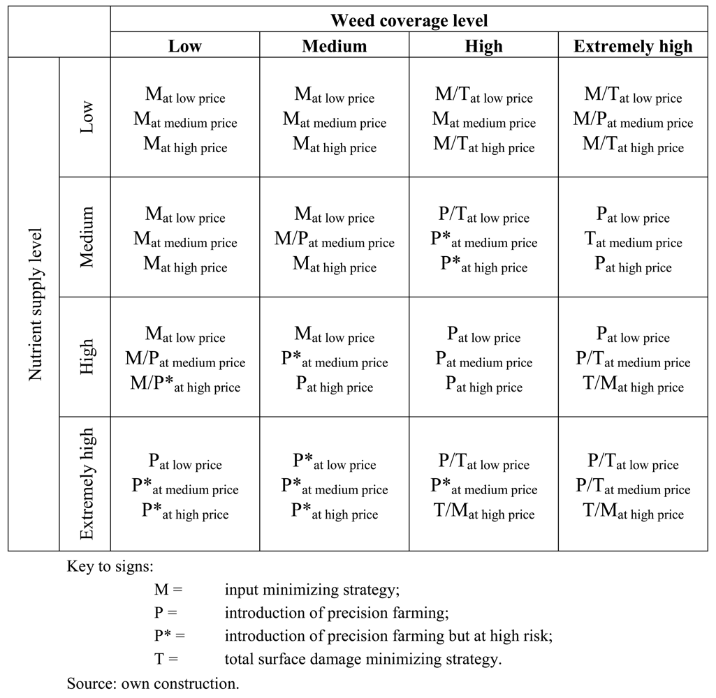
The signs of the analyzed strategies are the following:
<list list-type="bullet">
<list-item>
<p><italic>M</italic>: minimizing the treatment expenditures strategy (input minimizing);</p></list-item>
<list-item>
<p><italic>P</italic>: plant protection strategy;</p></list-item>
<list-item>
<p><italic>T</italic>: total surface treatment strategy.</p></list-item></list></p>
<p>Criteria of the implementation of the precision plant protection strategy (<italic>P</italic>) (<italic>B</italic> means benefit or net income of technology according to Equation (20)):
<disp-formula id="FD25">
<label>(25)</label>
<mml:math id="mm31" display="block">
<mml:semantics id="sm31">
<mml:mrow>
<mml:msup>
<mml:mi>B</mml:mi>
<mml:mi>P</mml:mi></mml:msup>
<mml:mo>≥</mml:mo>
<mml:msup>
<mml:mi>B</mml:mi>
<mml:mi>M</mml:mi></mml:msup></mml:mrow></mml:semantics></mml:math></disp-formula></p>
<p>The economic evaluation of precision technology is improving along with the increasing heterogeneity of the plot. The quitting point of precision farming is the point where the plot-level profit becomes negative. From this point forward, no economic advantage can be realized by applying precision technology, but it should be noted that during production decision making, other preferences could be considered other than economical. The suggested strategy after reaching the quitting point is the total surface treatment (<italic>T</italic>), damage control strategy. The determination base for this—the quitting threshold—can be described with the following relation:
<disp-formula id="FD26">
<label>(26)</label>
<mml:math id="mm32" display="block">
<mml:semantics id="sm32">
<mml:mrow>
<mml:msup>
<mml:mi>B</mml:mi>
<mml:mi>P</mml:mi></mml:msup>
<mml:mo>≤</mml:mo>
<mml:msup>
<mml:mi>B</mml:mi>
<mml:mi>T</mml:mi></mml:msup></mml:mrow></mml:semantics></mml:math></disp-formula></p>
<p>
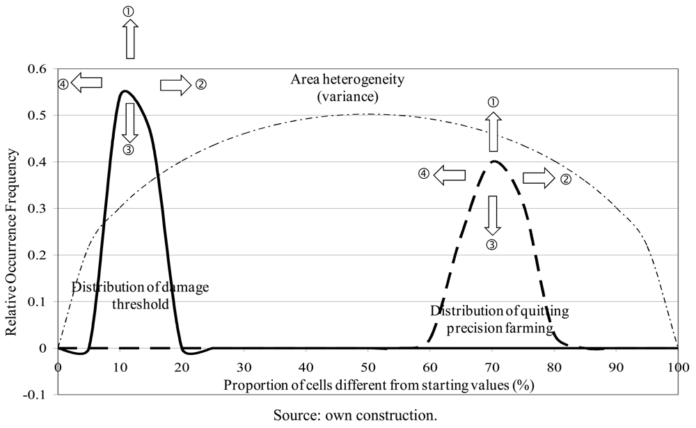
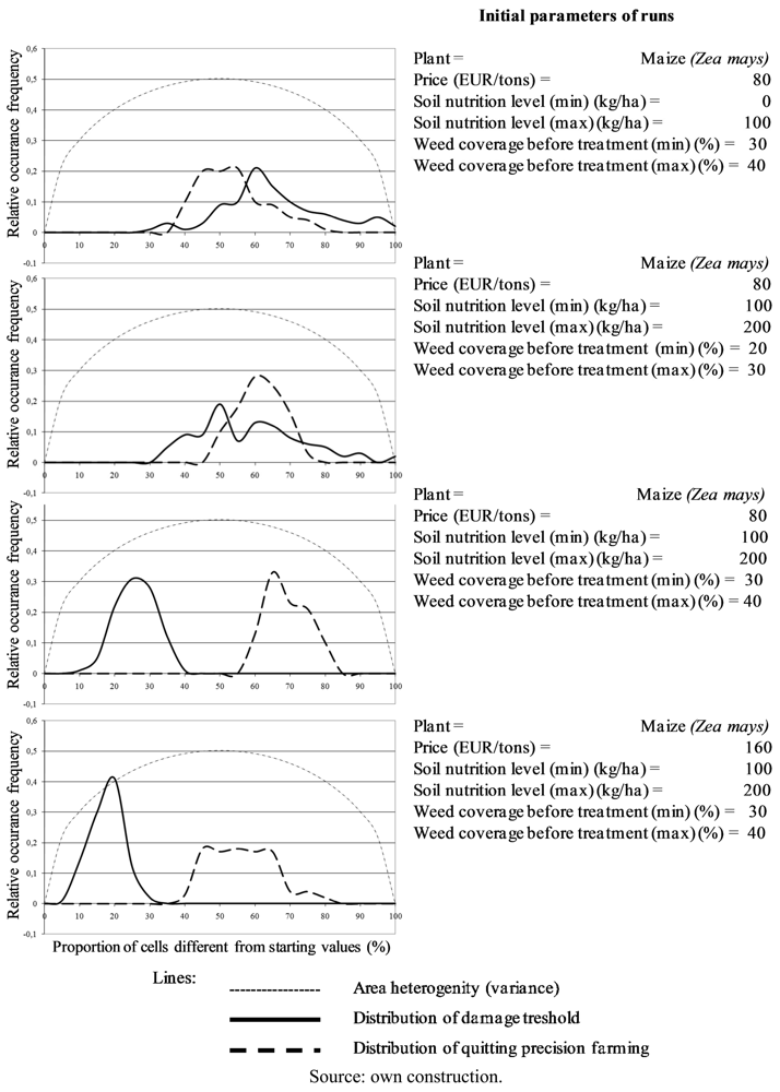
Based on the deterministic relations that serve as the setting of threshold values, we created a stochastic simulation model for further examinations. The uneven weed coverage and the uneven nutrition level were viewed as a yield influencing factor. The model did not investigate other risk factors, such as weather, pest damage, <italic>etc.</italic> The risk was understood, such as unfavorable events for the farmer (resulting in un-returnable investment of the new technologies' introduction), and it's frequency of appearance probability. The threshold values occurred with different frequencies in the model. The results of one running of the simulation are shown in <xref ref-type="fig" rid="f4-sustainability-03-01114">Figures 4</xref> and <xref ref-type="fig" rid="f5-sustainability-03-01114">5</xref>.</p>
<p>Two dispersion curves appear in the figure: According to our experiences in running the model (see sample results of runs in <xref ref-type="fig" rid="f4-sustainability-03-01114">Figure 4</xref>.), the location of the medium value of the dispersion curve and the peak of the dispersion curve are influenced by the nutrient level and the weed coverage of the area according to <xref ref-type="table" rid="t3-sustainability-03-01114">Table 3</xref> (<xref ref-type="table" rid="t3-sustainability-03-01114">Table 3</xref>, <xref ref-type="fig" rid="f5-sustainability-03-01114">Figure 5</xref>)</p></sec></sec>
<sec>
<label>3.</label>
<title>Experimental Section</title>
<sec>
<label>3.1.</label>
<title>Defining the Economic Damage and Quitting Threshold</title>
<p>We have examined the economic suitability and risk of precision crop production—focusing primarily on precision weed control—with the help of the aforementioned simulation model, in the cases of winter wheat, maize and sunflower. The value of the damage and the quitting threshold for switching to precision farming varies according to the intensity of production, the weed coverage and their heterogeneity within the plot. The model was run at three nutrient supply levels as well as three weed coverage levels, in case of three (low, average and high) sale prices, examining the economic suitability of precision technology for each crop. During the economic evaluation there was no difference made between precision nutrient supply and precision weed control, presuming that these two elements of technology are introduced together. In evaluating results, the precision nutrient supply in a technological sense is applied according to the heterogeneity of soil qualities, the precision weed control and its economical efficiency and applicability being different in each crop culture. Reasons for the differentiation are reliant upon the narrow or wide row distances, the crop weed suppression potential, and the difference in potential crop loss due to potential weeds.</p>
<p>In case of low nutrient supply and low weed coverage, the precision technology is not worth implementing, due to the differentiated, additional costs of the precision technique nutrient, and weed control application cannot be compensated with a similar amount on the return side. The rise of the need for additional nutrient supply and the degree of weed coverage will increase the viability of the spot treatments in an economic sense. In case of high nutrient supply level, an economic advantage (higher income) can be realized by comparing the cost of differentiated spreading and the value of yield surplus. On the other hand, in the case of increasing weed coverage, the value of yield saved due to spot treatments covers the extra costs of precision weed control. When a high nutrient supply level is paired with high weed coverage, the economic advantage of precision technology can be only proved when the heterogeneity of the area is high, while in case of a homogenous area (balanced soil–nutrient supply–weed coverage) undifferentiated treatment is more economical. The reason for this can be, on one hand, that in these cases there are fewer plots where no weed control is necessary, or on the other hand, that there are fewer plots where treatment is needed. The figure below describes the general rules (as an easily learned and an easily applied procedure for approximate estimation) for possible strategies, <xref ref-type="fig" rid="f6-sustainability-03-01114">Figure 6</xref>. Where two alternative strategies were assigned the results of simulation runs did not give the significant differences between the probabilities of the recommended strategies.</p>
<p>In the range with higher risk, the implementation of precision technology is influenced by the experience of the farmer and depends on the risk-toleration of the decision-maker.</p></sec>
<sec>
<label>3.2.</label>
<title>Changes on Weed Management Strategies</title>
<p>
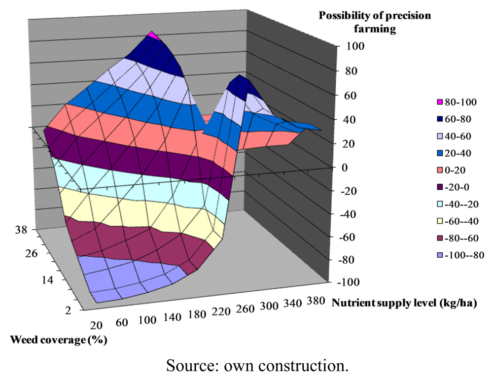
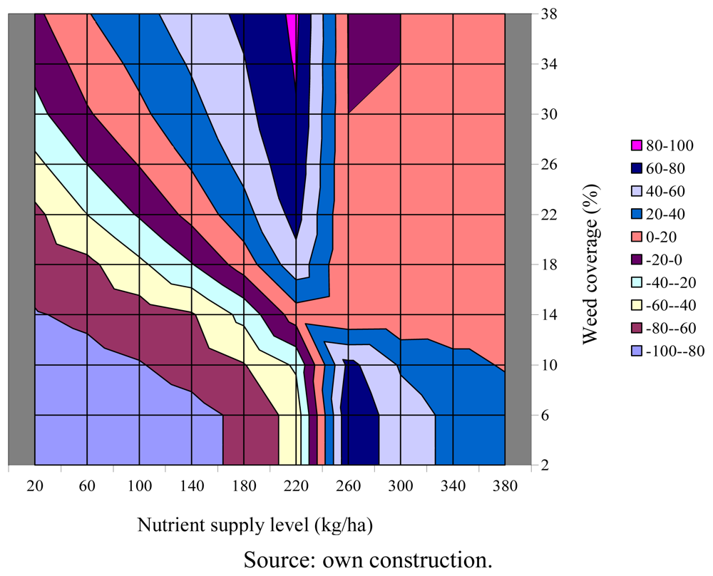
Hereinafter, using maize as an example, the changes of economic reasonability and the risks of farming strategies are introduced on the basis of relationships between nutrient supply level, weed coverage and sale prices.</p>
<p>In case of maize, at low sale prices (30.000 HUF/t), with low weed coverage, at minimum weed control costs, the precision technology is worthwhile economically only in cases of the highest nutrient supply level. In cases of medium and high nutrient supply, paired with high or very high weed coverage, the precision technique can yield higher income over the total surface treatment. In case of low nutrient level and high weed coverage it is not worthwhile economically to use precision treatment because the income from extra yield does not cover the extra costs required for the implementation of this technology. In case of low nutrient level and high weed coverage, the economically justifiable strategy is undifferentiated treatment made on the total surface and the minimization of costs.</p>
<p>When the sale price for maize increases precision crop production can be economically viable with intensive nutrient supply along with low or medium weed coverage, although the risk is high, similarly to the high (20–30%) weed coverage. The implementation of this strategy depends on the individual preferences, risk toleration and environmental consciousness of farmers. Even if the necessary technical background is available, it is not suggested to invest in the precision farming due to high risks at these cases. Presuming high sales prices, accompanied by high nutrient supply levels with medium and high weed coverage, precision crop production is economically viable. Although with the reduction of the nutrient supply level, the precision technology does not give higher results except in cases of very high weed coverage. When the sale prices increase, the extra material costs of whole-surface undifferentiated treatment are returned and it gives higher total income than the precision technology (<xref ref-type="fig" rid="f7-sustainability-03-01114">Figures 7</xref> and <xref ref-type="fig" rid="f8-sustainability-03-01114">8</xref>).</p>
<p>Presuming high sale prices, at high nutrient supply levels with medium or high weed coverage, precision crop production is economically reasonable. However, when the nutrient supply level decreases, the precision technology does not give higher results, except in cases of very high weed coverage. When the sale prices increase, the extra material costs of whole-surface undifferentiated treatment are returned, and it gives higher total income than precision technology. The higher the sale price, the narrower the range is in which this technology has economic viability.</p>
<p>The profitable implementation of precision technology for different crops depends on the soil nutrient supply level, the nutrient reaction of the crop under the given supply (input-output relation), the weed coverage, competition, extra costs of technology, and/or cost savings. The economic advantage of precision technology can be observed in the case of a technology that also includes weed control, if the heterogeneity of the area is large. This can be possible, because in this case significant areas of plots may not require weed control; therefore the material saving can be significant. In case of homogenous plot (uniform soil nutrition level, and weed coverage) the amount of those plots will be reduced that require no, or different weed control treatment. In this case, the whole-surface, undifferentiated treatment is the most economical. This, of course, does not exclude the implementation of precision technology in these cases—considering its positive, but currently not always measurable advantages, and its role in reducing environmental loads—but it should be accepted that in this case, extra income will not be realized at farm level. At the same time we should highlight the long-term advantages of precision technology, which is rooted in the environmental load reduction that is achieved by locally specified spreading.</p></sec>
<sec>
<label>3.3.</label>
<title>Risks of Precision Plant Protection</title>
<p>In consideration of introducing precision farming (damage threshold) and quitting (quitting threshold), the following statements could be made about the risks of the technology in connection with the production value, nutrient level and weed coverage:
<list list-type="alpha-upper">
<list-item>
<p>With the growth in output produced on the unit area, the damage threshold is reduced (the medium value of the damage threshold dispersion curve moves to the left), and the quitting threshold also moves to the left and levels out (the frequency of medium values decreases). The dispersion curve describing typically normal dispersion characteristics widens, which increases the risk of estimating quitting value; thus making it more difficult to predict its place.</p></list-item>
<list-item>
<p>By analyzing the nutrient impact, it can be stated that increasing the nutrient dose causes movements in two directions. The medium value of the damage threshold dispersion function moves to the left and tapers out (the frequency belonging to medium value increases). The same movement can be observed in the case of quitting threshold, but it will move to the right. To sum it up, the distance between the medium values of damage threshold and quitting threshold increase, widening the range of precision farming. This means that considering soil characteristics, the risk of switching to precision technology decreases when the production intensity is increased from the nutrient supply side. (It should be noted that this outcome proves and explains the fact that farms choosing precision crop production usually operate at higher production levels, and their annual yield fluctuations are smaller than the national average.)</p></list-item>
<list-item>
<p>In the case of low weed coverage, the frequency belonging to both threshold medium value decreases (the dispersion curve will be lower), and the medium value of damage threshold moves to the right while the quitting threshold value moves to the left. The dispersion of thresholds is characterless; the normal dispersion does not appear characteristically. When the weed coverage increases, the dispersion curves of threshold values attain normal dispersion characteristics, and the medium value of damage threshold shifts to the left, while the medium value of quitting threshold goes to the right. Increasing weed coverage widens the interval where economic advantage can be achieved from precision farming and reduces its risks. Under the examined economic condition system it means that the implementation of precision technology including its weed control element, at low or medium yield income has high risks, and is not justified economically in cases of low weed coverage.</p></list-item></list></p>
<p>The above examinations proved that the economic viability of precision farming depends on the yield that can be reached, the qualities of the production site, its heterogeneity and nutrient supply level, as well as the weed coverage and heterogeneity in the area. The higher production value and nutrient supply level (intensity) that can be achieved, justifies the implementation of precision crop production (widens the applicability) and reduces the risks. The increasing level of the weed coverage—which creates an unfavorable situation for the farmer—has a similar effect, reducing the risk of the precision technique. In connection with the returns gained in switching to precision farming, as stated earlier, the risks depend on the heterogeneity of soil and weed coverage. The risk matrix— which has been set up as a result of findings of the research's simulation model—shows the risk of returns, following the switch to the new technology [<xref ref-type="bibr" rid="b26-sustainability-03-01114">26</xref>]. In the case of low weed coverage, weed control is not necessary until the damage threshold is reached. Its place and size depends significantly on the actual sale price, and can be determined by the cell base, based on the relationship between the value of yield losses and the costs associated with the treatment of the given cell. If the weed coverage is high, the number of those cells where treatment can be omitted is low and the treatment of the total surface is suggested. In this case, the costs of extra investment connected with precision weed control should be examined. If the “saved output value” owing to the precision weed management throughout the duration does not cover the extra costs, the investment does not pay off. Of course, the technology can still be implemented in this case too, but actual savings on nutrient use cannot be expected. If neither of the above two cases are valid, precision weed management pays off in an economic sense also, in addition to its role in the reduction of environmental load. (<xref ref-type="table" rid="t4-sustainability-03-01114">Table 4</xref>)</p></sec></sec>
<sec sec-type="conclusions">
<label>4.</label>
<title>Conclusions</title>
<p>Precision crop production is a method which ensures economic sustainability. In order to prove it at the production level, the returns of extra investment required for the technology switch should be ensured in order to minimize the risk of switching. With an appropriate size and farming intensity, precision crop production is a real, environmentally conscious farming strategy, which with the help of the improved income can be realized, and it can ensure the economic conditions of simple re-production. Its risk is affected by: input/output prices differently, their changes compared to each other, the farm size (equipment from own investment or external services), production structure (crop varieties, their proportion), objectives of precision farming (heterogeneous–homogenous yield), heterogeneity of areas (nutrient supply, weed coverage), and expertise (preciseness and willingness).</p>
<p>Former examinations have proven that precision crop protection—primarily weed control—is the element of precision technology in which the risk is higher, in contrast to the switch to precision nutrient supply. The soil qualities (nutrient supply level, humus content, density) and the heterogeneity of weed coverage significantly affect those technological elements, where input can be saved and/or extra input is needed. Four basic strategies can be distinguished at the farmer's level from an economic perspective: 1. input minimizing, 2. precision farming, 3. high-risk precision farming, and 4. damage minimizing strategy with total surface treatment.</p>
<p>In addition to economical reasonability, the implementation of precision technology can also be justified by other factors. The first of which we refer to here is its role in the reduction of environmental loads. The further examination of this issue is another research direction, especially which questions play a role within the producers' individual decision. From this aspect, it is a method which simultaneously ensures ecological and economic sustainability. However, in our opinion this aspect is less emphasized among farmers' motivations, than in cases of switching to biological farming. Due to the related extra investment, including the high level of expertise and precision needed as described above and because of a lot of other factors unknown by the farmers, they will not switch to precision farming, solely and exclusively based on philosophical impulses. The viability of precision farming has already been proved in countries with developed agriculture. Its implementation in countries and regions with a segmented farm structure can be encouraged with cooperation within the framework of machine rings, similar to cooperatives, because in this way the criteria of size economics can be met.</p></sec></body>
<back>
<sec sec-type="display-objects">
<title>Figures and Tables</title>
<fig id="f1-sustainability-03-01114" position="float">
<label>Figure 1.</label>
<caption>
<p>Dimension of sustainability from the economic and social point of view.</p></caption>
<graphic xlink:href="sustainability-03-01114f1.gif"/></fig>
<fig id="f2-sustainability-03-01114" position="float">
<label>Figure 2.</label>
<caption>
<p>Decision criteria for treatment strategies, according to production function types (Cost-Income-Revenue (net income) structure).</p></caption>
<graphic xlink:href="sustainability-03-01114f2.gif"/></fig>
<fig id="f3-sustainability-03-01114" position="float">
<label>Figure 3.</label>
<caption>
<p>Determination of economically justified range of precision farming according to damage threshold (entering threshold) and upper limit (quitting threshold).</p></caption>
<graphic xlink:href="sustainability-03-01114f3.gif"/></fig>
<fig id="f4-sustainability-03-01114" position="float">
<label>Figure 4.</label>
<caption>
<p>Sample runs of simulation model for examining effects of price, soil nutrition level, weed coverage and their variability.</p></caption>
<graphic xlink:href="sustainability-03-01114f4.gif"/></fig>
<fig id="f5-sustainability-03-01114" position="float">
<label>Figure 5.</label>
<caption>
<p>Economically justified application range of precision farming and the possible movement directions of dispersion peaks.</p></caption>
<graphic xlink:href="sustainability-03-01114f5.gif"/></fig>
<fig id="f6-sustainability-03-01114" position="float">
<label>Figure 6.</label>
<caption>
<p>General rules of implementing weed management strategies (in maize).</p></caption>
<graphic xlink:href="sustainability-03-01114f6.gif"/></fig>
<fig id="f7-sustainability-03-01114" position="float">
<label>Figure 7.</label>
<caption>
<p>Distance between the damage threshold and quitting threshold according to nutrient supply level and weed coverage: maize (weed coverage 0–40%, nutrient supply level 0–400 kg/ha) (3D surface figure).</p></caption>
<graphic xlink:href="sustainability-03-01114f7.gif"/></fig>
<fig id="f8-sustainability-03-01114" position="float">
<label>Figure 8.</label>
<caption>
<p>Distance between the damage threshold and quitting threshold according to the nutrient supply level and weed coverage: maize (weed coverage 0–40%, nutrient supply level 0–400 kg/ha) (plan figure).</p></caption>
<graphic xlink:href="sustainability-03-01114f8.gif"/></fig>
<table-wrap id="t1-sustainability-03-01114" position="float">
<label>Table 1.</label>
<caption>
<p>Coefficients of yield function.</p></caption>
<table frame="box" rules="all">
<thead>
<tr>
<th align="center" valign="middle" rowspan="3">Culture</th>
<th colspan="6" align="center" valign="top"><bold>Coefficient</bold></th></tr>
<tr>
<th colspan="3" align="center" valign="middle">Yield depending on nutrition</th>
<th colspan="3" align="left" valign="middle">Correction coefficient of yield reduction depending on weed coverage</th></tr>
<tr>
<th align="center" valign="top">α</th>
<th align="center" valign="top">β</th>
<th align="center" valign="top">γ</th>
<th align="center" valign="top">κ</th>
<th align="center" valign="top">λ</th>
<th align="center" valign="top">μ</th></tr></thead>
<tbody>
<tr>
<td align="center" valign="top">Winter wheat</td>
<td align="center" valign="top">−0,000030</td>
<td align="center" valign="top">0,022</td>
<td align="center" valign="top">3,4</td>
<td align="center" valign="top">−0,0517</td>
<td align="center" valign="top">-2,2420</td>
<td align="center" valign="top">0</td></tr>
<tr>
<td align="center" valign="top">Maize</td>
<td align="center" valign="top">−0,000110</td>
<td align="center" valign="top">0,055</td>
<td align="center" valign="top">3,5</td>
<td align="center" valign="top">−0,0766</td>
<td align="center" valign="top">0,1416</td>
<td align="center" valign="top">0</td></tr>
<tr>
<td align="center" valign="top">Sunflower</td>
<td align="center" valign="top">−0,000050</td>
<td align="center" valign="top">0,016</td>
<td align="center" valign="top">2,1983</td>
<td align="center" valign="top">−0,0766</td>
<td align="center" valign="top">0,1416</td>
<td align="center" valign="top">0</td></tr></tbody></table>
<table-wrap-foot><fn id="tfn1-sustainability-03-01114">
<p>Source: own construction.</p></fn></table-wrap-foot></table-wrap>
<table-wrap id="t2-sustainability-03-01114" position="float">
<label>Table 2.</label>
<caption>
<p>Parameters of initial technological variants, on cells level (data from the simulation model).</p></caption>
<table frame="box" rules="all">
<thead>
<tr>
<th align="left" valign="middle" rowspan="2"><bold>Denomination</bold></th>
<th align="center" valign="middle" rowspan="2"><bold>Units of measurement</bold></th>
<th colspan="3" align="center" valign="top"><bold>Culture</bold></th></tr>
<tr>
<th align="center" valign="top"><bold>Winter wheat</bold></th>
<th align="center" valign="top"><bold>Maize</bold></th>
<th align="center" valign="top"><bold>Sunflower</bold></th></tr></thead>
<tbody>
<tr>
<td align="left" valign="top">Minimum price</td>
<td align="left" valign="top">c. u.<xref ref-type="table-fn" rid="tfn2-sustainability-03-01114">*</xref>/t</td>
<td align="left" valign="top">15,000</td>
<td align="left" valign="top">20,000</td>
<td align="left" valign="top">60,000</td></tr>
<tr>
<td align="left" valign="top">Maximum price</td>
<td align="left" valign="top">c. u./t</td>
<td align="left" valign="top">60,000</td>
<td align="left" valign="top">120,000</td></tr>
<tr>
<td align="left" valign="top">Size of cells</td>
<td align="left" valign="top">ha</td>
<td align="left" valign="top">0.01</td>
<td align="left" valign="top">0.01</td></tr>
<tr>
<td align="left" valign="top">Unit cost of fertilizer</td>
<td align="left" valign="top">c. u./kg</td>
<td align="left" valign="top">120</td>
<td align="left" valign="top">120</td></tr>
<tr>
<td align="left" valign="top">Cost of weed management by 1% weed coverage</td>
<td align="left" valign="top">c. u./ha</td>
<td align="left" valign="top">800</td>
<td align="left" valign="top">1500</td>
<td align="left" valign="top">2000</td></tr>
<tr>
<td align="left" valign="top">Seed cost</td>
<td align="left" valign="top">c. u./cell<xref ref-type="table-fn" rid="tfn3-sustainability-03-01114">**</xref></td>
<td align="left" valign="top">130</td>
<td align="left" valign="top">233</td>
<td align="left" valign="top">164</td></tr>
<tr>
<td align="left" valign="top">Equipment cost (variable)</td>
<td align="left" valign="top">c. u./cell</td>
<td align="left" valign="top">284</td>
<td align="left" valign="top">304</td>
<td align="left" valign="top">323</td></tr>
<tr>
<td align="left" valign="top">Cost of drying</td>
<td align="left" valign="top">c. u./t</td>
<td align="left" valign="top">368</td>
<td align="left" valign="top">2 014</td>
<td align="left" valign="top">889</td></tr>
<tr>
<td align="left" valign="top">Specific fixed costs of conventional technology</td>
<td align="left" valign="top">c. u./cell</td>
<td align="left" valign="top">606</td>
<td align="left" valign="top">728</td>
<td align="left" valign="top">647</td></tr>
<tr>
<td align="left" valign="top">Specific fixed costs of precision technology</td>
<td align="left" valign="top">c. u./cell</td>
<td align="left" valign="top">702</td>
<td align="left" valign="top">846</td>
<td align="left" valign="top">747</td></tr></tbody></table>
<table-wrap-foot><fn id="tfn2-sustainability-03-01114">
<label>*</label>
<p>current unit: HUF;</p></fn><fn id="tfn3-sustainability-03-01114">
<label>**</label>
<p>cell is sampling plot.</p></fn><fn id="tfn4-sustainability-03-01114">
<p>Source: own construction.</p></fn></table-wrap-foot></table-wrap>
<table-wrap id="t3-sustainability-03-01114" position="float">
<label>Table 3.</label>
<caption>
<p>Direction of dispersion curves in relation to production value (output price), nutrient level and weed coverage.</p></caption>
<table frame="box" rules="all">
<thead>
<tr>
<th align="left" valign="bottom"><bold>Direction</bold></th>
<th align="center" valign="bottom"><bold>Damage threshold</bold></th>
<th align="center" valign="bottom"><bold>Quitting threshold</bold></th></tr></thead>
<tbody>
<tr>
<td align="left" valign="top">Production price is increasing</td>
<td align="center" valign="top">❶②③❹</td>
<td align="center" valign="top">❶②③❹</td></tr>
<tr>
<td align="left" valign="top">Weed coverage is increasing</td>
<td align="center" valign="top">❶②③❹</td>
<td align="center" valign="top">❶❷③④</td></tr>
<tr>
<td align="left" valign="top">Nutrient level is increasing</td>
<td align="center" valign="top">❶②③❹</td>
<td align="center" valign="top">❶❷③④</td></tr>
<tr>
<td align="left" valign="top">Nutrient level is increasing above the optimum of nutrient utilization function</td>
<td align="center" valign="top">①❷❸④</td>
<td align="center" valign="top">①❷❸④</td></tr>
<tr>
<td align="left" valign="top">Peak of yield function is increasing</td>
<td align="center" valign="top">①❷❸④</td>
<td align="center" valign="top">①❷❸④</td></tr></tbody></table>
<table-wrap-foot><fn id="tfn5-sustainability-03-01114">
<p>Note: direction of movements: ①❶: up, ②❷: to the right, ③❸: down, ④❹: to the left movement: movement is made in the direction indicated in dark;</p></fn><fn id="tfn6-sustainability-03-01114">
<p>Source: own construction.</p></fn></table-wrap-foot></table-wrap>
<table-wrap id="t4-sustainability-03-01114" position="float">
<label>Table 4.</label>
<caption>
<p>Risk of returns of switching to precision farming according to soil characteristics and weed coverage.</p></caption>
<table frame="box" rules="all">
<thead>
<tr>
<th align="left" valign="middle" rowspan="2"><bold>Heterogeneity of weed coverage</bold></th>
<th colspan="3" align="center" valign="top"><bold>Heterogeneity of soil characteristics</bold></th></tr>
<tr>
<th align="center" valign="top"><bold>Small</bold></th>
<th align="center" valign="top"><bold>Medium</bold></th>
<th align="center" valign="top"><bold>Large</bold></th></tr></thead>
<tbody>
<tr>
<td align="left" valign="top">Small</td>
<td align="center" valign="top">+++</td>
<td align="center" valign="top">++</td>
<td align="center" valign="top">+</td></tr>
<tr>
<td align="left" valign="top">Medium</td>
<td align="center" valign="top">++</td>
<td align="center" valign="top">+</td></tr>
<tr>
<td align="left" valign="top">Large</td>
<td align="center" valign="top">++</td>
<td align="center" valign="top">+</td>
<td align="center" valign="top">+</td></tr></tbody></table>
<table-wrap-foot><fn id="tfn7-sustainability-03-01114">
<p>Key to signs:
<list list-type="simple">
<list-item>
<p>+++high risk, no returns;</p></list-item>
<list-item>
<p>++medium risks, uncertain returns;</p></list-item>
<list-item>
<p>+low risk, probable returns.</p></list-item></list></p></fn><fn id="tfn8-sustainability-03-01114">
<p>Source: own construction.</p></fn></table-wrap-foot></table-wrap></sec>
<ref-list>
<title>References</title>
<ref id="b1-sustainability-03-01114"><label>1.</label><citation citation-type="book"><person-group person-group-type="author"><name><surname>Pearce</surname><given-names>D.</given-names></name><name><surname>Atkinson</surname><given-names>G.</given-names></name></person-group><article-title>Measuring of sustainable development</article-title><source>The Handbook of Environmental Economics</source><person-group person-group-type="editor"><name><surname>Bromly</surname><given-names>D.</given-names></name></person-group><publisher-name>Blackwell</publisher-name><publisher-loc>Cambridge, MA, USA</publisher-loc><year>1995</year><fpage>166</fpage><lpage>181</lpage></citation></ref>
<ref id="b2-sustainability-03-01114"><label>2.</label><citation citation-type="journal"><person-group person-group-type="author"><name><surname>Bongiovanni</surname><given-names>R.</given-names></name><name><surname>Lowengerg-DeBoer</surname><given-names>J.</given-names></name></person-group><article-title>Precision agriculture and sustainability</article-title><source>Precision Agric.</source><year>2004</year><volume>5</volume><fpage>359</fpage><lpage>387</lpage><pub-id pub-id-type="doi">10.1023/B:PRAG.0000040806.39604.aa</pub-id></citation></ref>
<ref id="b3-sustainability-03-01114"><label>3.</label><citation citation-type="book"><person-group person-group-type="author"><name><surname>Caffey</surname><given-names>R.H.</given-names></name><name><surname>Kazmierczak</surname><given-names>R.F.</given-names></name><name><surname>Avault</surname><given-names>J.W.</given-names></name></person-group><source>Incorporating Multiple Stakeholder Goals into the Development and use of Sustainable Index: Consensus Indicators of Aquaculture Sustainability.</source><comment>Staff Paper</comment><publisher-name>Department of AgEcon and Agribusiness of Louisiana State University</publisher-name><publisher-loc>Eunice, LA, USA</publisher-loc><month>August</month><year>2001</year><fpage>40</fpage></citation></ref>
<ref id="b4-sustainability-03-01114"><label>4.</label><citation citation-type="book"><person-group person-group-type="author"><name><surname>Csete</surname><given-names>L.</given-names></name><name><surname>Láng</surname><given-names>I.</given-names></name></person-group><source>A Fenntartható Agrárgazdaság És Vidékfejlesztés (Sustainable agriculture and rural development)</source><publisher-name>MTA Társadalomkutató Központ</publisher-name><publisher-loc>Budapest, Hungary</publisher-loc><year>2005</year><fpage>313</fpage></citation></ref>
<ref id="b5-sustainability-03-01114"><label>5.</label><citation citation-type="journal"><person-group person-group-type="author"><name><surname>Stull</surname><given-names>J.</given-names></name><name><surname>Dillon</surname><given-names>C.</given-names></name><name><surname>Shearer</surname><given-names>S.</given-names></name><name><surname>Isaacs</surname><given-names>S.</given-names></name></person-group><article-title>Using precision agriculture technology for economically optimal strategic decisions: The case of CRP filter strip enrollment</article-title><source>J. Sustainable Agric.</source><year>2004</year><volume>24</volume><fpage>79</fpage><lpage>96</lpage><pub-id pub-id-type="doi">10.1300/J064v24n04_07</pub-id></citation></ref>
<ref id="b6-sustainability-03-01114"><label>6.</label><citation citation-type="journal"><person-group person-group-type="author"><name><surname>Várallyay</surname><given-names>Gy.</given-names></name></person-group><article-title>Soil resilience (Is soil a renewable natural resource?)</article-title><source>Cereal Res. Commun.</source><year>2007</year><volume>35</volume><fpage>1277</fpage><lpage>1280</lpage><pub-id pub-id-type="doi">10.1556/CRC.35.2007.2.278</pub-id></citation></ref>
<ref id="b7-sustainability-03-01114"><label>7.</label><citation citation-type="journal"><person-group person-group-type="author"><name><surname>Mawapanga</surname><given-names>M.N.</given-names></name><name><surname>Debertin</surname><given-names>D.L.</given-names></name></person-group><article-title>Choosing between alternative farming systems: An application of the analytic hierarchy process</article-title><source>Rev. Agric. Econ.</source><year>1996</year><volume>18</volume><fpage>385</fpage><lpage>401</lpage></citation></ref>
<ref id="b8-sustainability-03-01114"><label>8.</label><citation citation-type="book"><person-group person-group-type="author"><name><surname>Michelsen</surname><given-names>J.</given-names></name></person-group><article-title>Organic farming development in Europe: Impacts of regulation and institutional diversity</article-title><source>Economics of Pesticides, Sustainable Food Production and Organic Food Markets</source><person-group person-group-type="editor"><name><surname>Hall</surname><given-names>D.C.</given-names></name><name><surname>Moffitt</surname><given-names>L.J.</given-names></name></person-group><publisher-name>Elsevier Science</publisher-name><publisher-loc>Amsterdam, The Netherlands</publisher-loc><year>2002</year><volume>4</volume><fpage>101</fpage><lpage>138</lpage></citation></ref>
<ref id="b9-sustainability-03-01114"><label>9.</label><citation citation-type="book"><person-group person-group-type="author"><name><surname>Takács</surname><given-names>I.</given-names></name></person-group><article-title>Az organikus termelés növekedésének modellezése a kereslet-kínálat és jövedelmezőség változás függvényében (Modelling of organic farming according to change of demand and supply as well as profitability)</article-title><source>Növényvédő szer használat csökkentés gazdasági hatásai (Economic effects of decreasing of pesticide using)</source><person-group person-group-type="editor"><name><surname>Takács-György</surname><given-names>K.</given-names></name></person-group><publisher-name>Szent István Egyetemi Kiadó</publisher-name><publisher-loc>Budapest, Hungary</publisher-loc><year>2006</year><fpage>135</fpage><lpage>148</lpage></citation></ref>
<ref id="b10-sustainability-03-01114"><label>10.</label><citation citation-type="confproc"><person-group person-group-type="author"><name><surname>Dillon</surname><given-names>C.R.</given-names></name><name><surname>Gandonou</surname><given-names>J.M.</given-names></name></person-group><article-title>Precision timing and spatial allocation of economic fertilizer application. Southern Agricultural Economics Association</article-title><conf-name>In proceedings of Southern Agricultural Economics Association, 2007 Annual Meeting</conf-name><conf-loc>Mobile, AL, USA</conf-loc><conf-date>February 4-7, 2007</conf-date></citation></ref>
<ref id="b11-sustainability-03-01114"><label>11.</label><citation citation-type="journal"><person-group person-group-type="author"><name><surname>Wolf</surname><given-names>S.A.</given-names></name><name><surname>Buttel</surname><given-names>F.H.</given-names></name></person-group><article-title>The political economy of precision farming</article-title><source>Am. J. Agric. Econ.</source><year>1996</year><volume>78</volume><fpage>1269</fpage><lpage>1274</lpage><pub-id pub-id-type="doi">10.2307/1243505</pub-id></citation></ref>
<ref id="b12-sustainability-03-01114"><label>12.</label><citation citation-type="journal"><person-group person-group-type="author"><name><surname>Auernhammer</surname><given-names>H.</given-names></name></person-group><article-title>Precision farming—the environmental challenge</article-title><source>Comput. Electron. Agric.</source><year>2001</year><volume>30</volume><fpage>31</fpage><lpage>43</lpage><pub-id pub-id-type="doi">10.1016/S0168-1699(00)00153-8</pub-id></citation></ref>
<ref id="b13-sustainability-03-01114"><label>13.</label><citation citation-type="journal"><person-group person-group-type="author"><name><surname>Chavas</surname><given-names>J.P.</given-names></name></person-group><article-title>A cost approach to economic analysis under state-contingent production uncertainty</article-title><source>Am. J. Agric. Econ.</source><year>2008</year><volume>90</volume><fpage>435</fpage><lpage>446</lpage><pub-id pub-id-type="doi">10.1111/j.1467-8276.2007.01118.x</pub-id></citation></ref>
<ref id="b14-sustainability-03-01114"><label>14.</label><citation citation-type="journal"><person-group person-group-type="author"><name><surname>Takács-György</surname><given-names>K.</given-names></name></person-group><article-title>Economic aspects of chemical reduction on farming: Role of precision farming–will the production structure change?</article-title><source>Cereal Res. Commun.</source><year>2008</year><volume>36</volume><fpage>19</fpage><lpage>22</lpage></citation></ref>
<ref id="b15-sustainability-03-01114"><label>15.</label><citation citation-type="confproc"><person-group person-group-type="author"><name><surname>Schnitkey</surname><given-names>G.</given-names></name><name><surname>Hopkins</surname><given-names>J.</given-names></name><name><surname>Tweeten</surname><given-names>L.</given-names></name></person-group><article-title>An economic evaluation of precision fertilizer applications on corn and soybean fields</article-title><conf-name>Presented at the AAEA Annual Meeting</conf-name><conf-loc>San Antonio, TX, USA</conf-loc><conf-date>July 1996</conf-date></citation></ref>
<ref id="b16-sustainability-03-01114"><label>16.</label><citation citation-type="journal"><person-group person-group-type="author"><name><surname>Weiss</surname><given-names>M.D.</given-names></name></person-group><article-title>Precision farming and spatial economic analysis: Research challenges and opportunities</article-title><source>Am. J. Agric. Econ.</source><year>1996</year><volume>78</volume><fpage>1275</fpage><lpage>1280</lpage><pub-id pub-id-type="doi">10.2307/1243506</pub-id></citation></ref>
<ref id="b17-sustainability-03-01114"><label>17.</label><citation citation-type="journal"><person-group person-group-type="author"><name><surname>Biermacher</surname><given-names>J.T.</given-names></name><name><surname>Epplin</surname><given-names>F.M.</given-names></name><name><surname>Brorsen</surname><given-names>B.W.</given-names></name><name><surname>Solie</surname><given-names>J.B.</given-names></name><name><surname>Raun</surname><given-names>W.R.</given-names></name></person-group><article-title>Economic feasibility of site-specific optical sensing for managing nitrogen fertilizer for growing wheat</article-title><source>Precis. Agric.</source><year>2009</year><volume>10</volume><fpage>213</fpage><lpage>230</lpage><pub-id pub-id-type="doi">10.1007/s11119-008-9092-y</pub-id></citation></ref>
<ref id="b18-sustainability-03-01114"><label>18.</label><citation citation-type="journal"><person-group person-group-type="author"><name><surname>Attanandana</surname><given-names>T.</given-names></name><name><surname>Yost</surname><given-names>R.</given-names></name><name><surname>Verapattananirund</surname><given-names>P.</given-names></name></person-group><article-title>Empowering Farmer Leaders to Acquire and Practice Site-Specific Nutrient Management Technology</article-title><source>J. Sustainable Agric.</source><year>2007</year><volume>30</volume><fpage>87</fpage><lpage>104</lpage></citation></ref>
<ref id="b19-sustainability-03-01114"><label>19.</label><citation citation-type="journal"><person-group person-group-type="author"><name><surname>Barroso</surname><given-names>J.</given-names></name><name><surname>Fernandez-Quintanilla</surname><given-names>C.</given-names></name><name><surname>Maxwell</surname><given-names>B.D.</given-names></name><name><surname>Rew</surname><given-names>L.J.</given-names></name></person-group><article-title>Simulating the effects of weed spatial pattern and resolution of mapping and spraying on economics of site-specific management</article-title><source>Weed Res.</source><year>2004</year><volume>44</volume><fpage>460</fpage><lpage>468</lpage><pub-id pub-id-type="doi">10.1111/j.1365-3180.2004.00423.x</pub-id></citation></ref>
<ref id="b20-sustainability-03-01114"><label>20.</label><citation citation-type="journal"><person-group person-group-type="author"><name><surname>Rider</surname><given-names>T.W.</given-names></name><name><surname>Vogel</surname><given-names>J.W.</given-names></name><name><surname>Dille</surname><given-names>J.A.</given-names></name><name><surname>Dhuyvetter</surname><given-names>K.C.</given-names></name><name><surname>Kastens</surname><given-names>T.L.</given-names></name></person-group><article-title>An economic evaluation of site-specific herbicide application</article-title><source>Precis. Agric.</source><year>2006</year><volume>7</volume><fpage>379</fpage><lpage>392</lpage><pub-id pub-id-type="doi">10.1007/s11119-006-9012-y</pub-id></citation></ref>
<ref id="b21-sustainability-03-01114"><label>21.</label><citation citation-type="journal"><person-group person-group-type="author"><name><surname>Gutjahr</surname><given-names>C.</given-names></name><name><surname>Weiss</surname><given-names>M.</given-names></name><name><surname>Sökfeld</surname><given-names>M.</given-names></name><name><surname>Ritter</surname><given-names>C.</given-names></name><name><surname>Möhring</surname><given-names>J.</given-names></name><name><surname>Büsche</surname><given-names>A.</given-names></name><name><surname>Piepho</surname><given-names>H.P.</given-names></name><name><surname>Gerhards</surname><given-names>R.</given-names></name></person-group><article-title>Erarbeitung von Entscheidungsalgoorithmen für die teilflächenspezifische Unkrautbekämpfung</article-title><source>J. Plant Dis. Prot.</source><year>2008</year><volume>21</volume><fpage>143</fpage><lpage>148</lpage></citation></ref>
<ref id="b22-sustainability-03-01114"><label>22.</label><citation citation-type="journal"><person-group person-group-type="author"><name><surname>Oriade</surname><given-names>C.</given-names></name><name><surname>King</surname><given-names>R.</given-names></name><name><surname>Forcella</surname><given-names>F.</given-names></name><name><surname>Gunsolus</surname><given-names>J.</given-names></name></person-group><article-title>A bioeconomic analyses of site-specific management for weed control</article-title><source>Rev. Agric. Econ.</source><year>1996</year><volume>18</volume><fpage>523</fpage><lpage>535</lpage></citation></ref>
<ref id="b23-sustainability-03-01114"><label>23.</label><citation citation-type="journal"><person-group person-group-type="author"><name><surname>Just</surname><given-names>R.E.</given-names></name></person-group><article-title>Risk research in agricultural economics: Opportunities and challenges for next twenty-five years</article-title><source>Agric. Syst.</source><year>2003</year><volume>75</volume><fpage>123</fpage><lpage>159</lpage><pub-id pub-id-type="doi">10.1016/S0308-521X(02)00063-X</pub-id></citation></ref>
<ref id="b24-sustainability-03-01114"><label>24.</label><citation citation-type="journal"><person-group person-group-type="author"><name><surname>Monjardino</surname><given-names>M.</given-names></name><name><surname>Pennel</surname><given-names>D.J.</given-names></name><name><surname>Powles</surname><given-names>S.B.</given-names></name></person-group><article-title>A multi-species bio-economic model for integrated weed management</article-title><source>Weed Sci.</source><year>2003</year><volume>51</volume><fpage>798</fpage><lpage>809</lpage><pub-id pub-id-type="doi">10.1614/P2002-118</pub-id></citation></ref>
<ref id="b25-sustainability-03-01114"><label>25.</label><citation citation-type="journal"><person-group person-group-type="author"><name><surname>Takács-György</surname><given-names>K.</given-names></name><name><surname>Reisinger</surname><given-names>P.</given-names></name><name><surname>Takács</surname><given-names>E.</given-names></name><name><surname>Takács</surname><given-names>I.</given-names></name></person-group><article-title>Economic analysis of precision plant protection by stochastic simulation based on finite elements method</article-title><source>J. Plant Dis. Prot.</source><year>2008</year><volume>21</volume><fpage>181</fpage><lpage>186</lpage></citation></ref>
<ref id="b26-sustainability-03-01114"><label>26.</label><citation citation-type="journal"><person-group person-group-type="author"><name><surname>Takács-György</surname><given-names>K.</given-names></name><name><surname>Takács</surname><given-names>I.</given-names></name></person-group><article-title>Analysis of farm-level decision criteria of introducing precision plant protection</article-title><source>Cereal Res. Commun.</source><year>2009</year><volume>37</volume><fpage>573</fpage><lpage>576</lpage></citation></ref></ref-list></back></article>
