Optimization of a Groundwater Monitoring Network for a Sustainable Development of the Maheshwaram Catchment, India


Abstract
: Groundwater is one of the most valuable resources for drinking water and irrigation in the Maheshwaram Catchment, Central India, where most of the local population depends on it for agricultural activities. An increasing demand for irrigation and the growing concern about potential water contamination makes imperative the implementation of a systematic groundwater-quality monitoring program in the region. Nonetheless, limited funding and resources emphasize the need to achieve a representative but cost-effective sampling strategy. In this context, field observations were combined with a geostatistical analysis to define an optimized monitoring network able to provide sufficient and non-redundant information on key hydrochemical parameters. A factor analysis was used to evaluate the interrelationship among variables, and permitted to reduce the original dataset into a new configuration of monitoring points still able to capture the spatial variability in the groundwater quality of the basin. The approach is useful to maximize data collection and contributes to better manage the allocation of resources under budget constrains.1. Introduction
Industrial production and agriculture are major threats to water resources in the semi arid regions of India. In recent years groundwater provided water to irrigate approximately 27 million hectares (60% of the country's irrigated land) against 21 million hectares supplied by surface water [1]. Between 1970 and 1994, the extent of groundwater-irrigated land in India increased by 105%, whilst land irrigated by surface waters showed an increase of only 28% [2]. At many localities, groundwater constitutes the only supply for drinking purposes. The dramatic increase in groundwater usage clearly shows that competition for water is on the rise. Furthermore, climate change and population growth in years to come are expected to place additional pressure on the groundwater system. Planning and an adequate management of the resources are crucial not only to meet the demand, but also to protect the water quality of stressed regions.
The first step of any sustainable management is to understand the underlying physical processes and to derive the corresponding mathematical formulations [3]. In the Maheshwaram Catchment, there is a large number of irrigation bores useful for monitoring purposes. However, constrains on budget, equipment, and human resources mean that only on a limited number of these bores can be used for investigation. Selecting the location of the points to be monitored involves practical and technical considerations but to a certain extent, the process is subjected to bias and uncertainty. In this regard, geostatistical predictions are being increasingly used to address the imperfect knowledge of attributes that fluctuate over large areas [4]. The accuracy of the data retrieved and the subsequent predictions are especially dependant on a reliable optimization of the monitoring network. The information generated by such an optimal monitoring network should provide sufficient and non-redundant information to fully understand the spatial phenomena of the monitored variables. Several statistical methods can be applied to approach the problem. According to [5], these methods can be classified as simulations, variance-based techniques, and probability. Essentially, the difference among them lies in the formulation of the objective function to be optimized. The variance reduction method is widely accepted as a reliable tool in optimization problems [2]. In addition, it usually requires less iterations to obtain the same accuracy on the estimates. The technique utilizes a unique property of geostatistical estimation by which the variance of the estimation error depends only on the structure of the selected parameter and not on the measured values at additional points. This enables one to select a new observation point and analyze its effect prior to making a measurement [6]. Due to these advantages, the variance reduction technique was selected for the present exercise. The uncertainty associated with a given monitoring network may be determined by the variance of estimation obtained by kriging interpolation. In a certain area, the uncertainty for a distribution of monitoring wells is associated to that particular location. Changes in the number or location of wells will be directly reflected in the level of accuracy of the estimations. Thus, the variance of the error must be sought to be used as an objective function.
This paper describes the use of geostatistical techniques on groundwater-quality data in the Maheshwaram Catchment, India, in order to determine an optimal monitoring network for the area. The approach is essentially supported by a principal component analysis (PCA) along with kriging interpolation. Findings from the study are useful to reduce the existing dataset whilst retaining the relationships originally present. More importantly, the optimized network constitutes a cost-effective alternative to design future sampling programs, and allows for a better management of the available resources under budgetary constrains.
2. Theoretical Considerations
The principal component analysis (PCA) is a procedure for finding hypothetical variables which account for the majority of the variance in a multi-dimensional dataset [7]. This can be achieved by transforming the variables under study into a new set of variables, the principal components (PCs). Thus, the goal when using PCA analysis is to determine a few linear combinations of the original variables that can be used to summarize the dataset without losing much information [8]. The mathematics behind the procedure is explained in most statistic textbooks and will not be presented here. However, it is worthy to note that the analysis calculates new variables from the original variables in an attempt to detect similarities among the original data. The method allows for the identification of homogeneous subgroups that better describe the system behavior [9].
Quantification of the spatio-temporal variability of a dataset can be achieved by the use of variograms. A generalized formula to calculate a variogram from a set of scattered data can be written as follows [10]:
On the other hand, kriging is a method for linear optimum unbiased interpolation with a minimum mean interpolation error [11]. Kriging is only a technique among many others for interpolation of a variable. However, it presents a number of advantages since it considers: (i) the number and spatial configuration of observation points; (ii) the position of the data points; (iii) the distance between the data points with respect to the area of interest; and (iv) the spatial continuity of the interpolated variable [12]. These advantages and its wide application in hydrogeological problems led us to select this method for the present study.
In short, kriging is a method of weighted averaging of the observed values of a property Z within a neighborhood V, from measured values z(xi) of the property at ‘n’ sites, xi = 1,2,3, …, n. Estimates can be made over a block B by:
3. Study Area
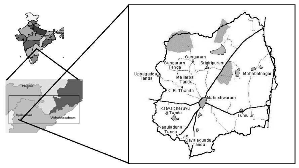
The Maheshwaram catchment is located approximately 30 km south of Hyderabad, in the Ranga Reddy district of Andra Pradesh, India (Figure 1). The area is a typical granitic terrain extending over an area of about 60 km2.
The topography is flat to gently undulating, with elevations between 590 and 670 m above mean sea level. The climate is classified as semi-arid, with a mean annual precipitation in the order of 750 mm, mainly falling during the monsoon season between June and September. There are no perennial streams. On a regional scale, groundwater flows from SW to NE.
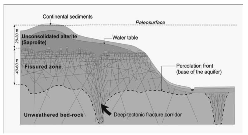
Geologically, the area is dominated by Archean granites of medium to coarse grain, commonly intruded by quartz and dolerite dykes over several generations. Rocks have undergone a variable degree of weathering, usually with a thickness of 15 m to 20 m. An underlying fractured zone extends up to 50 m below ground level (mbgl) (Figure 2). Crystalline basement aquifers can be divided in several compartments that together constitute the aquifer but which are characterized by distinct hydrogeological properties [13,14]. In the area of study, these compartments can be described as: (i) the upper zone which consists of weathered and decayed rocks of clayey-sandy composition. Their hydraulic conductivity is usually low, but ther water-retention capacity can be significant; (ii) the intermediate fissured zone (FZ) characterized by horizontal fractures that diminish in density with depth, and an important number of vertical fractures and fissures that act as preferential pathways. This zone is characterized by higher values of hydraulic conductivity; (iii) the underlying unaltered rock, usually of low permeability and limited storage capacity.
4. Methods
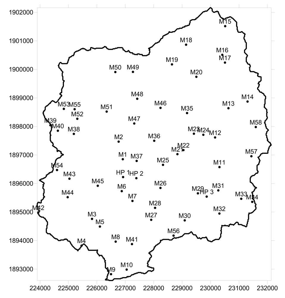
A PCA analysis was carried out on groundwater-quality data from 61 bores scattered throughout the Maheshwaram catchment (Figure 3). Data collection involved both field and laboratory work. Standard parameters such as electrical conductivity (EC), and pH were measured in situ. Samples were taken following parameters stabilization. Water was filtered in the field and stored in previously-rinsed 500 ml bottles for chemical tests. A subset of samples was acidified with HNO3 for cation analyses. Anions such as SO42−, Cl−, NO32−, F−, and PO42− were analyzed using a Dionex DX-2500 ion chromatograph. Cations (Ca2+, Mg2+, Cu+, Fe2+, K+) were determined by atomic absorption spectrometry at the NGRI facilities in Hyderabad. Bicarbonate (HCO3−) was estimated by titration, whilst TDS and total hardness were measured with manual meters.
5. Results and Discussion
A correlation matrix was used to apply a PCA analysis of water quality data. Following the methodology of [15], components with an eigenvalue less than 1 were eliminated. Thus, only the first three components were extracted for the analysis. The initial factors solution was then rotated by the variamax rotation technique [16], in order to obtain new variables (i.e., principal components or principal axes). As indicated by their cumulative percentage of variance, the three extracted components accounted for 62% of the entire dataset variance (Appendix I).
The first factor explained 37% of the total variance. It was characterized by very high loadings of TDS and EC, high loadings of SO42− and Cl−, and somewhat moderate Na+ and total hardness. These results suggest that the above mentioned ions are the main solutes in groundwater, and are thus, responsible for the elevated dissolved solids and conductivity values present in the system. Leakage of agricultural products would dominate the input of these chemicals into groundwater.
In contrast, the combination of factors 2 and 3 contribute to nearly 25% of the total variance. Factor 2 is characterized by high pH, alkalinity, and F- loadings, whilst factor 3 is dominated by Ca2+, Fe2+, Mg2+, and moderate K+ and hardness. It is hypothesized that these elements are derived from natural processes rather than anthropogenic activities.
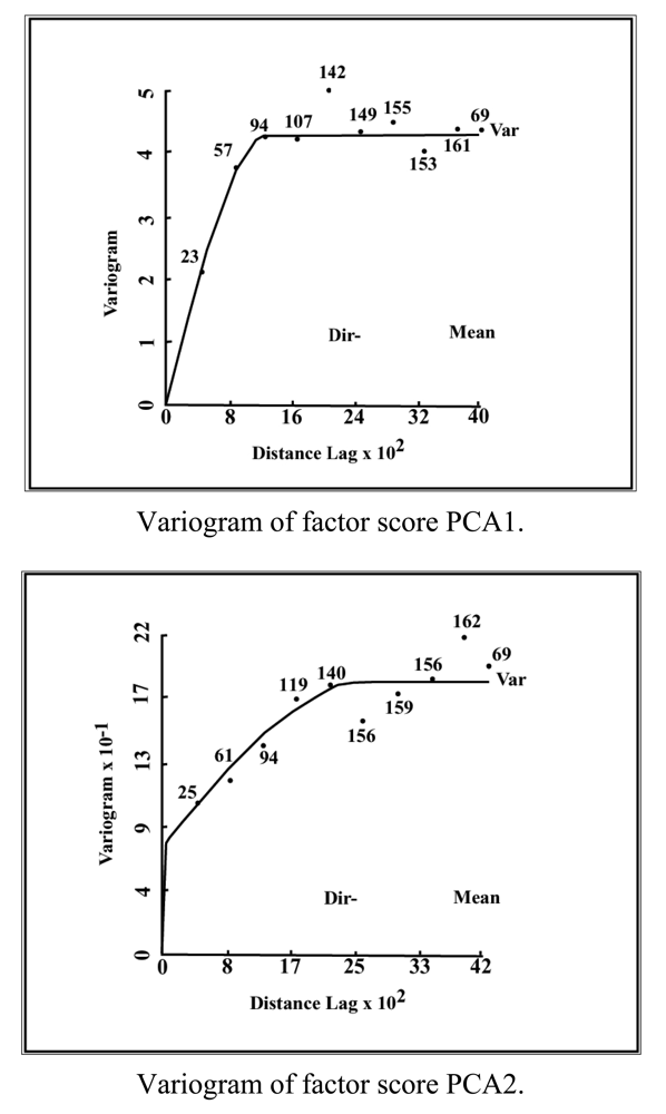
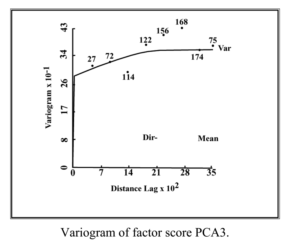
The three principal components of the PCA (PC1, PC2, PC3) were used to establish three new variables (X1, X2, X3), which project the ‘n’ observations onto the first three principal components. These new variables constituted the basis for optimizing the monitoring network with a reduced number of interrelated variables. The spatial variability of these new variables over the Maheshwaram watershed was defined by calculating their experimental and theoretical variograms (Appendix II). Before the implementation of any simulation or optimization mathematical model, consistency with the original data must be verified [17]. Thus, a cross validation test was carried out to ensure that the variogram represents the true variability of the parameter and is able to reproduce the measured values:
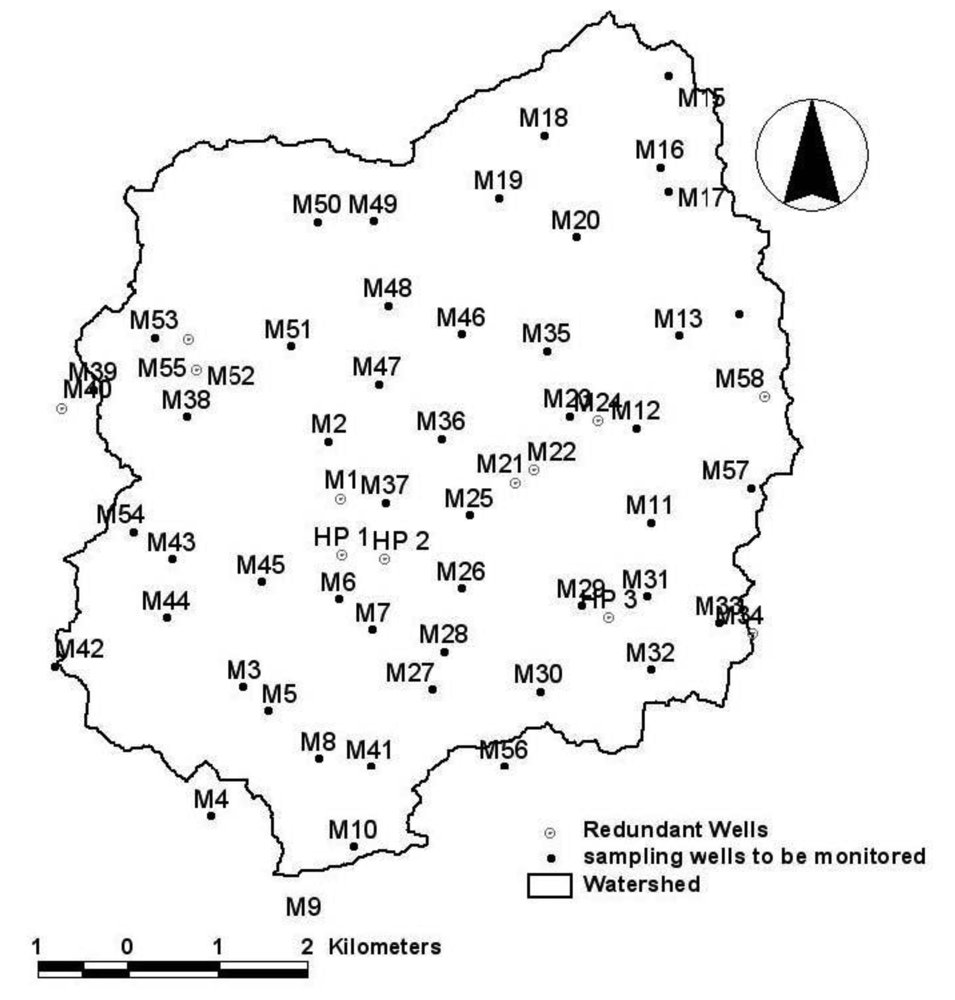
The cross validation was performed by masking a specified value from the dataset and then estimating it from the remaining values and by the variograms. Results must satisfy Equation (11) otherwise, the variogram outcomes cannot be considered plausible. Having established the adequacy of the variograms, the kriging procedure was employed to estimate the standard error across the area of investigation. The watershed was divided into a uniform grid of 883 cells of 250 m by side and a cut-off value of 0.5 was established for the first variable. In contrast, values of 0.7 and 1 were considered for the second and third variable respectively. Points were individually removed to see their effect on the error function. Points that resulted into an increase of the estimation error if removed were kept in the monitoring network. In contrast, boreholes that did not affect the error value were permanently eliminated. This procedure was repeated for each one of the three variables, to finally derive an optimized monitoring network through combination of points. A spatial distribution of redundant wells is depicted in Figure 4. The original dataset and the optimized monitoring network produced similar solutions, which lead to the conclusion that a reduction in the number of observation points does not compromise the quality and resolution of the collected samples if the network distribution is properly designed (Table 1).
As a last validation, the final monitoring network was examined against each one of the 15 initial variables. The verification procedure does not aim to prove the correctness of the model but to ensure the absence of systematic errors [11,18]. This was carried out by making variographic analysis of all the initial parameters. Cross validation tests were performed and then followed by the ordinary kriging estimation of each variable using original observation points and optimized monitoring points. Estimations were carried out on 250 m grids for both the original and final monitoring network. Subsequently, the mean standard deviation of the estimation error was calculated. Results of the analysis confirm the redundancy of 13 points for each of the individual initial parameters (Table 2).
6. Summary and Conclusions
Identification of aquifer parameters by direct observations is a challenging task. The distribution of measurement points depends on a number of factors such as aquifer characteristics, terrain conditions, and availability of resources. Heterogeneous conditions usually require a dense monitoring network, which in most cases is not economically feasible. As a consequence, complex groundwater systems must be analyzed from only a handful of observations. It is clear that the accuracy of the inferences made is strongly linked to the arrangement of the observation points. A correct well distribution needs to capture a representative set of aquifer properties that can be extrapolated to unsampled locations. Experience and technical knowledge play a major role in the process, but to a certain extent, selecting the wells location is inherently subjective. Therefore, the last years have witnessed an increase in the use of geostatistical techniques to quantitatively evaluate and optimize observation networks. In this context, a PCA analysis was applied to water-quality data of the Maheshwaram catchment, India, to optimize the groundwater monitoring network in the region. Kriging interpolation provided an insight into the uncertainty of the distribution. Results indicated that 13 out of a total of 61 bores are redundant and therefore, should be disregarded in future sampling rounds. A comparison between the interpolation error of the original dataset and the optimized distribution showed a negligible difference. This indicates that a reduction in the number of monitoring wells will not incur in a considerable loss of detail for data collected in the future. In view of this, it is concluded that an efficient sampling network should not be defined solely on intuition or qualitative assessments as they can be misleading. Through a simple exercise, the present study demonstrated that an adequate configuration of observation points is still able to accurately capture the spatial variability of groundwater characteristics, while maximizing the use of the allocated resources. The continuous development of more user-friendly software and the reduction in computational efforts suggest that the use of geostatistical tools will increase in the future, allowing hydrogeologists to better reach an appropriate trade-off between density of data and the investment demanded to collect it.


| Factor 1 | Factor 2 | Factor 3 | |
|---|---|---|---|
| Monitoring Wells* | HP 1, HP 2, HP 3, M1, M4, M9, M21, M22, M23, M24, M34, M40, M52, M55, M56, M58 | HP 1, HP2, HP 3, M1, M9, M21, M22, M24, M34, M40, M52, M55, M58 | HP 1, HP 2, HP 3, M1, M5, M6, M7, M9, M21, M22, M23, M24, M28, M34, M40, M52, M55, M58 |
| MSD of Kriging estimation error (initial monitoring network) | 1.15 | 0.91 | 1.08 |
| Sum of squared difference (initial monitoring network) | 13.6 | 0.25 | 1.76 |
| MSD of Kriging estimation error (after optimization) | 1.16 | 0.91 | 1.08 |
| Sum of squared difference (after optimization) | 13.8 | 0.25 | 1.8 |
*Redundant monitoring wells in bold italics; MSD: mean standard deviation.
| Original monitoring network | Optimized monitoring network | |||
|---|---|---|---|---|
| Parameter | Mean standard deviation of kriging estimation error | Sum of squared difference | Mean standard deviation of kriging estimation error | Sum of squared difference |
| Calcium | 0.7 | 48 | 0.7 | 48 |
| pH | 0.1 | 3 | 0.1 | 3 |
| EC | 2 | 0 | 2 | 0 |
| Sulfate | 27 | 13 | 27 | 13 |
| Alkalinity | 99 | 542 | 99 | 541 |
| Chlorine | 57 | 734 | 57 | 730 |
| Nitrate | 0 | 0.2 | 0 | 0.2 |
| Carbonate | 89 | 203 | 89 | 201 |
| Fluorine | 0.8 | 21 | 0.8 | 22 |
| Magnesium | 19 | 259 | 19 | 263 |
| Copper | 0.7 | 86 | 0.7 | 88 |
| Iron | 3 | 1.5 | 3 | 1.5 |
| Phosphate | 2 | 34 | 2 | 35 |
| TDS | 76 | 108 | 76 | 107 |
| Hardness | 14 | 86 | 13.5 | 88 |
Acknowledgments
The authors are grateful to Sheryl Ryan and Jo Searle, Groundwater Review Section, Department of Water of Western Australia for the review and assistance in improving the manuscript.
Appendix
| Well ID. | Well Name | X (m) | Y (m) | PCA 1 (Factor score) | PCA 2 (Factor score) | PCA 3 (Factor score) |
|---|---|---|---|---|---|---|
| 1 | HP 1 | 226,921 | 1,896,226 | 1.0 | 0.2 | 0.3 |
| 2 | HP 2 | 227,388 | 1,896,187 | 5.1 | −0.4 | 0.8 |
| 3 | HP 3 | 229,864 | 1,895,542 | 5.7 | −0.4 | 1.4 |
| 4 | M1 | 226,911 | 1,896,852 | 3.1 | −0.8 | 1.4 |
| 5 | M2 | 226,765 | 1,897,468 | 2.2 | −0.1 | −1.4 |
| 6 | M3 | 225,827 | 1,894,760 | −1.6 | −2.0 | −0.9 |
| 7 | M4 | 225,460 | 1,893,324 | −2.8 | −1.1 | −1.1 |
| 8 | M5 | 226,105 | 1,894,492 | −1.8 | −0.9 | −0.8 |
| 9 | M6 | 226,874 | 1,895,733 | −1.1 | −2.3 | 0.9 |
| 10 | M7 | 227,251 | 1,895,390 | −2.7 | −1.3 | −0.9 |
| 11 | M8 | 226,660 | 1,893,964 | −0.5 | −0.5 | −1.0 |
| 12 | M9 | 226,496 | 1,892,123 | −2.3 | −1.7 | −0.2 |
| 13 | M10 | 227,047 | 1,892,984 | −0.3 | −1.9 | 0.0 |
| 14 | M11 | 230,314 | 1,896,576 | −1.0 | −0.8 | −0.4 |
| 15 | M12 | 230,160 | 1,897,614 | −2.4 | −1.1 | −1.3 |
| 16 | M13 | 230,630 | 1,898,639 | 1.3 | −1.0 | 1.2 |
| 17 | M14 | 231,303 | 1,898,873 | −1.6 | −0.3 | −0.6 |
| 18 | M15 | 230,515 | 1,901,515 | 1.7 | −1.0 | 1.0 |
| 19 | M16 | 230,414 | 1,900,510 | 1.4 | −1.8 | 1.8 |
| 20 | M17 | 230,508 | 1,900,238 | 2.7 | −2.0 | 0.4 |
| 21 | M18 | 229,139 | 1,900,865 | 5.2 | −0.6 | 0.2 |
| 22 | M19 | 228,642 | 1,900,175 | −0.4 | −0.1 | −1.4 |
| 23 | M20 | 229,501 | 1,899,740 | 6.2 | −0.4 | −1.1 |
| 24 | M21 | 228,834 | 1,897,029 | −1.7 | −0.1 | −0.3 |
| 25 | M22 | 229,046 | 1,897,172 | −0.5 | −1.4 | −0.4 |
| 26 | M23 | 229,414 | 1,897,746 | −0.4 | 0.8 | −1.0 |
| 27 | M24 | 229,746 | 1,897,708 | −0.7 | 1.3 | −0.6 |
| 28 | M25 | 228,326 | 1,896,654 | −2.1 | −0.5 | −0.1 |
| 29 | M26 | 228,236 | 1,895,845 | −1.3 | −0.7 | 0.7 |
| 30 | M27 | 227,911 | 1,894,728 | −2.0 | 1.1 | −1.2 |
| 31 | M28 | 228,047 | 1,895,147 | −2.0 | −0.3 | −0.4 |
| 32 | M29 | 229,555 | 1,895,656 | 1.9 | −1.3 | 1.9 |
| 33 | M30 | 229,091 | 1,894,708 | −2.1 | −1.6 | −1.2 |
| 34 | M31 | 230,273 | 1,895,759 | −0.9 | 0.4 | 0.0 |
| 35 | M32 | 230,312 | 1,894,948 | 0.1 | −0.1 | 0.3 |
| 36 | M33 | 231,081 | 1,895,465 | −2.1 | −0.5 | −0.4 |
| 37 | M34 | 231,468 | 1,895,357 | −1.9 | −0.3 | −0.8 |
| 38 | M35 | 229,173 | 1,898,469 | 1.8 | 3.4 | −1.3 |
| 39 | M36 | 228,017 | 1,897,499 | −0.5 | 0.9 | 0.9 |
| 40 | M37 | 227,399 | 1,896,792 | 3.0 | 0.4 | 1.7 |
| 41 | M38 | 225,187 | 1,897,739 | 0.4 | 1.9 | −1.2 |
| 42 | M39 | 224,162 | 1,898,042 | −1.5 | −0.7 | −1.0 |
| 43 | M40 | 223,825 | 1,897,850 | −0.8 | 3.8 | −1.5 |
| 44 | M41 | 227,234 | 1,893,877 | −2.1 | 0.0 | −0.6 |
| 45 | M42 | 223,735 | 1,894,985 | −2.1 | −0.5 | −0.8 |
| 46 | M43 | 225,032 | 1,896,169 | 0.2 | 3.6 | −0.1 |
| 47 | M44 | 224,970 | 1,895,521 | 0.1 | 1.0 | −0.4 |
| 48 | M45 | 226,030 | 1,895,921 | −0.7 | 0.4 | 0.0 |
| 49 | M46 | 228,238 | 1,898,651 | −1.0 | −1.1 | −1.4 |
| 50 | M47 | 227,314 | 1,898,104 | 0.9 | −0.2 | −1.1 |
| 51 | M48 | 227,419 | 1,898,970 | 0.5 | 1.2 | −1.7 |
| 52 | M49 | 227,268 | 1,899,912 | −0.3 | −0.2 | −0.7 |
| 53 | M50 | 226,648 | 1,899,907 | −0.4 | 1.6 | 0.0 |
| 54 | M51 | 226,343 | 1,898,521 | 4.8 | 1.7 | 0.3 |
| 55 | M52 | 225,309 | 1,898,269 | 0.2 | 0.3 | −0.1 |
| 56 | M53 | 224,835 | 1,898,616 | −1.2 | −0.2 | 0.2 |
| 57 | M54 | 224,595 | 1,896,473 | −0.3 | 4.0 | −1.0 |
| 58 | M55 | 225,215 | 1,898,604 | −0.3 | 1.3 | 0.1 |
| 59 | M56 | 228,698 | 1,893,874 | −1.2 | 0.4 | −0.6 |
| 60 | M57 | 231,438 | 1,896,956 | −0.9 | 2.4 | 0.2 |
| 61 | M58 | 231,593 | 1,897,979 | 0.13 | 0.05 | −0.38 |
| Percentage of variance | 37.4 | 15.5 | 9.5 | |||
References
- Roy, A.D.; Shah, C. Socio-ecology of groundwater irrigation in India. In Intensive Use of Groundwater. Challenges and Opportunities; Llamas, R., Custodio, E., Eds.; Taylor & Francis: Lisse, The Netherlands, 2002; pp. 307–335. [Google Scholar]
- Zaidi, F.K.; Ahmed, S.; Dewandel, B.; Marechal, J.C. Optimizing a piezometric network in the estimation of the groundwater budget: A case study from a crystalline-rock watershed in southern India. Hydrogeol. J. 2007, 15, 1131–1145. [Google Scholar]
- Qahman, K.; Larabi, A.; Ouazar, D.; Naji, A.; Cheng, A.H.D. Optimal and sustainable extraction of groundwater in coastal aquifers. Stoch. Environ. Res. Risk Assess. 2005, 19, 99–110. [Google Scholar]
- Olea, R. A six-step statistical approach to semivariagram modeling. Stoch. Environ. Res. Risk Assess. 2006, 20, 307–318. [Google Scholar]
- Loaiciga, H.A.; Charbeneau, R.J.; Everett, L.G.; Fogg, G.E.; Hobbs, B.F.; Rouhani, S. Review of ground-water quality monitoring network design. J. Hydraul. Eng. 1992, 118, 11–37. [Google Scholar]
- Agnihotri, V.; Ahmed, S. Analyzing ambiguities in the data collection network design by geostatistical estimation variance reduction method. J. Environ. Hydrol. 1997, 5, 1–13. [Google Scholar]
- Harper, D.A.T. Numerical Palaeobiology; John Wiley & Sons: New York, NY, USA, 1999. [Google Scholar]
- Winter, T.; Mallory, S.; Allen, T.; Rosenberry, D. The use of principal component analysis for interpreting ground water hydrographs. Ground Water 2000, 38, 234–246. [Google Scholar]
- Mellinger, M. Multivariate data analysis: Its methods. Chemometr. Intell. Lab. Syst. 1987, 2, 29–36. [Google Scholar]
- Ahmed, S. An interactive software for computation and modeling of a variogram. Proceedings of the Conference on Water Resources Management, Isfahan, Iran; 1995; pp. 797–808. [Google Scholar]
- Theodossiou, N.; Latinopoulus, P. Evaluation and optimisation of groundwater observation networks using the Kriging methodology. Environ. Modell. Softw. 2006, 21, 991–1000. [Google Scholar]
- Aboufirassi, M.; Mariño, M.A. Kriging of water levels in the Souss Aquifer, Morocco. Math. Geol. 1983, 15, 537–551. [Google Scholar]
- Lachassagne, P.; Pinault, J.-L. Radon-222 emanometry: A relevant methodology for water well sitting in hard rock aquifer. Water Resour. Res. 2001, 37, 3131–3148. [Google Scholar]
- Wyns, R.; Baltassat, J.M.; Lachassagne, P.; Legtchenko, A.; Vairon, J. Application of proton magnetic resonance soundings to groundwater reserves mapping in weathered basement rocks (Brittany, France). Bulletin de la Société Géologique de France 2004, 175, 21–34. [Google Scholar]
- Chatfield, C.; Collins, A.J. Introduction to Multivariate Analysis; Chapman & Hall (CRC Texts in Statistical Science); CRC Press: New York, NY, USA, 1980. [Google Scholar]
- Kaisher, H.F. The varimax criterion for analytic rotation in factor analysis. Psychometrika 1958, 23, 187–200. [Google Scholar]
- Hill, M.C.; Banta, E/R.; Harbaugh, A.W.; Anderman, E.R. MODFLOW-2000. In The USGS Modular Ground-Water Model—User Guide to the Observation, Sensitivity, and Parameter Estimation Processes; Open File Report 00-184; USGS: Reston, VA, USA, 2000. [Google Scholar]
- Jolly, W.M.; Graham, J.M.; Michaelis, A.; Nemani, R.; Running, S.W. A flexible, integrated system for generating meteorological surfaces derived from point sources across multiple geographic scales. Environ. Modell. Softw. 2005, 20, 873–882. [Google Scholar]
© 2011 by the authors; licensee MDPI, Basel, Switzerland. This article is an open access article distributed under the terms and conditions of the Creative Commons Attribution license (http://creativecommons.org/licenses/by/3.0/).
Share and Cite
Nabi, A.; Gallardo, A.H.; Ahmed, S. Optimization of a Groundwater Monitoring Network for a Sustainable Development of the Maheshwaram Catchment, India. Sustainability 2011, 3, 396-409. https://doi.org/10.3390/su3020396
Nabi A, Gallardo AH, Ahmed S. Optimization of a Groundwater Monitoring Network for a Sustainable Development of the Maheshwaram Catchment, India. Sustainability. 2011; 3(2):396-409. https://doi.org/10.3390/su3020396
Chicago/Turabian StyleNabi, Aadil, Adrian H. Gallardo, and Shakeel Ahmed. 2011. "Optimization of a Groundwater Monitoring Network for a Sustainable Development of the Maheshwaram Catchment, India" Sustainability 3, no. 2: 396-409. https://doi.org/10.3390/su3020396