Article

Sustainable Zero-Valent Metal (ZVM) Water Treatment Associated with Diffusion, Infiltration, Abstraction, and Recirculation

DCA Consultants Ltd., Haughend Farm, Bridge of Earn Road, Dunning, Perthshire, PH2 9BX, Scotland, UK
Sustainability 2010, 2(9), 2988-3073; https://doi.org/10.3390/su2092988
Submission received: 10 August 2010 / Revised: 28 August 2010 / Accepted: 13 September 2010 / Published: 17 September 2010

Abstract

:
Socio-economic, climate and agricultural stress on water resources have resulted in increased global demand for water while at the same time the proportion of potential water resources which are adversely affected by sodification/salinisation, metals, nitrates, and organic chemicals has increased. Nano-zero-valent metal (n-ZVM) injection or placement in aquifers offers a potential partial solution. However, n-ZVM application results in a substantial reduction in aquifer permeability, which in turn can reduce the amount of water that can be abstracted from the aquifer. This study using static diffusion and continuous flow reactors containing n-ZVM and m-ZVM (ZVM filaments, filings and punchings) has established that the use of m-ZVM does not result in a reduction in aquifer permeability. The experimental results are used to design and model m-ZVM treatment programs for an aquifer (using recirculation or static diffusion). They also provide a predictive model for water quality associated with specific abstraction rates and infiltration/injection into an aquifer. The study demonstrates that m-ZVM treatment requires 1% of the weight required for n-ZVM treatment for a specific flow rate. It is observed that 1 t Fe0 will process 23,500 m3 of abstracted or infiltrating water. m-ZVM is able to remove >80% of nitrates from flowing water and adjust the water composition (by reduction) in an aquifer to optimize removal of nitrates, metals and organic compounds. The experiments demonstrate that ZVM treatment of an aquifer can be used to reduce groundwater salinity by 20 –> 45% and that an aquifer remediation program can be designed to desalinate an aquifer. Modeling indicates that widespread application of m-ZVM water treatment may reduce global socio-economic, climate and agricultural stress on water resources. The rate of oxygen formation during water reduction [by ZVM (Fe0, Al0 and Cu0)] controls aquifer permeability, the associated aquifer pH, aquifer Eh and the degree of water treatment that occurs.

Graphical Abstract

1. Introduction

Contaminated and untreated water is present in confined/unconfined aquifers, groundwater plumes, groundwater mounds (GWM), self-sealing groundwater mounds, storm runoff, riparian systems, and abstracted well/borehole water. The reservoir rock/sediment may provide a low cost, sustainable, basic level of natural water treatment but can add natural contaminants (e.g., As). Contaminants include organic chemicals, metals, foul pollutants, industrial waste and agricultural waste (e.g., nitrates). They may result from anthropogenic activities (e.g., agriculture, industrial activity, over-development, poor sanitation drainage, etc.). They can be a natural consequence of water abstraction from inappropriate water sources (e.g., abstraction from aquifers enriched in As, Pb, etc.). They may result from leaching from the surrounding host rock when over-abstraction from an aquifer occurs. Abstraction and usage of polluted/contaminated waters may create health problems and may reduce the sustainability of the land for use in agriculture.
Water in aquifers may be contained in large open systems (covering >100 km2) or may occur as more local closed water bodies covering small spatial areas of between <1,000 m2 to 1 km2). The requirement by many national environment agencies for developers and drainage/water authorities to use sustainable urban drainage systems (SUDS) to dispose of storm runoff water, grey water and foul water complicates the natural situation. This policy can result in dispersed infiltration of contaminated water into the subsoil. This infiltrating water may leach metals, nitrates, sulphates, salts and organic chemicals into the underlying aquifers and may contaminate regional aquifers [1]. The contaminated aquifers, particularly in irrigation areas, may become more saline [1].
A natural consequence of SUDS drainage directed to infiltration is the formation of contaminated groundwater plumes within aquifers, contaminated GWMs, and contaminated self-sealing groundwater mounds. Groundwater plumes and contaminated groundwater mounds are semi-open systems with diffuse boundaries, which may migrate with time [1]. Self-sealing GWMs are sealed perched water body systems with defined boundaries [1,2].
Sustainable water treatment is a multi-disciplinary and holistic approach, which integrates technical, environmental, economic, landscape, societal, political, religious, and cultural issues. Technical research guides the appropriate strategies and policies used to implement sustainable aquifer/water treatment. Recharge of aquifers/GWMs and riparian discharge in SUDS requires an assessment [1,2] of overland flow and infiltration/aquifer recharge associated with specific design storms (e.g., 24 h) with specific return periods (e.g., 10 years, 50 years, 100 years, etc.). Sustainable environmental and planning policies require drainage developments (including pollution discharge) to be able to meet specific environmental standards provided the overland flow is associated with a design storm with a return period of <x years.
These policies require remediation of polluted plumes and GWM/aquifers. This remediation is designed to protect downstream aquifers and allow abstraction from (or development over) the polluted plume/GWM. Polluted infiltrating water associated with storm recharge flowing through contaminated soil will continually recharge many contaminated plumes/GWM.
Sustainable Zero-Valent Metal (ZVM) water treatment associated with infiltration, abstraction, and recirculation removes metals (including As), nitrates, chloro-organics, sulphates, phosphates, organic chemicals) from water in the aquifer/GWM (or during abstraction/infiltration). ZVM treatment is experimental [3,4,5,6,7,8,9,10,11,12,13,14,15,16,17], but offers the potential to treat storm runoff, abstracted water and water within an aquifer. The experimental focus has been to identify if n-ZVM treatment actually reduces pollutants Where the ZVM treatment is effective the experimental studies have sought to identify the kinetic parameters associated with pollutant removal [5], i.e., the relationship between temperature and the rate of pollutant removal.
These ZVM studies do not allow prediction at a remediation design phase of the timescale associated with the remediation program, the amount of pollutant removed from the aquifer as a function of time, or the expected variation in pollutant removal from storm water runoff (overland flow) as a function of specific design storms. They are therefore difficult to directly integrate into the design of a sustainable remediation program or SUDS.
This study addresses the specific SUDS remediation/treatment design issues by using experimental data to create a series of regression equations (Eh, pH, EC), which can be used to quantitatively predict the performance of a ZVM remediation program or SUDS as a function of time, ZVM quantity and flow rate. Application of the regression relationships in design modeling for SUDS projects and GWM/plume remediation allows the treatment provided by ZVM to be directly related to:
  • specific design storms for storm runoff,
  • abstraction/infiltration/runoff flow rate,
  • the amount of ZVM placed in an aquifer for static diffusion treatment (and time), and
  • the abstraction and infiltration/injection rate when aquifer/plume/GWM treatment strategy requires the entire Eh and pH of the water body to be changed to new defined limits.
These experimental results provide a basis for the quantitative design of sustainable m-ZVM treatment programs, which can provide:
  • treated drinking water (including removal of leached metals, micro-organisms, and organic chemicals),
  • remediated GWMs and plumes,
  • treated GWMs and plumes to support specific agriculture activities and remove the adverse effects of leaching/infiltration of pollutants,
  • improved water quality in aquifers, and
  • low cost, rapid supply, high volume sources of treated water in the aftermath of natural/ anthropogenic disasters.

1.1. ZVM Treatment

Historically two approaches have been used to treat groundwater using nano-ZVM (n-ZVM). They are:
  • the creation of permeable reactive barriers (PRB) containing n-ZVM (e.g., a physical static barrier within the aquifer containing n-ZVM) [5,8,9,10,11,12,13,14,15] and
  • the injection of n-ZVM into an aquifer with injected or infiltrating water [6,7,16,17].
n-ZVM has a low permeability [8], which decreases with time [15] due to recrystallisation within the n-ZVM bed [15] and the development of pore occlusion by O2(g) [1,2,18,19,20]. Injected/infiltrating n-ZVM reduces aquifer permeability by particle clogging of pores, pore throat radii reduction, and increasing flow path tortuosity [6,21]. The reduction of water by the ZVM produces O2(g) [22].
Spent n-ZVM is difficult to recover from an infiltration device, PRB, or well, due to its small particle size. m-ZVM is immobile and can be recovered from a surface or subsurface continuous flow or static diffusion reactor (or PRB or infiltration device or well). The term m-ZVM is used to define micron/millimeter sized ZVM [e.g., fine filaments (Figure 1)], which are immobile under the prevailing driving force, ΔP, Pa. The term n-ZVM is used to define ZVM powder (Figure 2) with a grain size of <60,000 nm (Figure 2).
Figure 1. m-ZVM (a) m-Fe0 filaments. Field of view = 5 cm. (b) m-Cu0 filaments. Field of view = 3 cm. (c) m-Al0 punchings. Punching diameter = 5 mm.
Sustainability 02 02988 g001
Figure 2. n-ZVM powder. (a) n-Fe0. (b) n-Cu0. (c) n-Al0.
Sustainability 02 02988 g002

1.2. Sustainable ZVM Treatment Design Issues Addressed

The implementation and design issues addressed are:
1 n-ZVM (Figure 2) in a continuous flow reactor
a. What is the magnitude of permeability reduction with time?
Three continuous flow reactors (DR1 to DR3) containing n-ZVM were operated with a constant driving force for a period of 90 days (Figure 3). The test results indicate flow rate reductions through the n-ZVM of 98–99%.
b. What is the magnitude of the Eh and pH changes and do they change with space velocity as the flow rate through the n-ZVM declines?
The DR1 to DR3 test results define a series of regression relationships, which vary with ZVM type and space velocity.
c. Can continuous flow through n-ZVM be used to effectively treat water by modifying the Eh and pH environment?
Modeling (of aquifer redox transformation) using the experimental regression relationships is compared with the results from a pilot n-ZVM injection program into a contaminated groundwater plume. The regression relationships provide a modeled redox environment, which is similar to the redox environment observed in the pilot injection program.
2 m-ZVM (Figure 1) in a continuous flow reactor
a. What is the magnitude of permeability reduction with time?
Three continuous flow reactors (BR1 to BR3) containing m-ZVM were operated with a constant driving force until the ZVM ceased to be effective (Figure 4). The test results indicate that there is no reduction in flow rate or permeability with time, and that the m-ZVM permeability (Figure 4) is higher than the initial permeability through n-ZVM (Figure 3).
b. What is the magnitude of the Eh and pH changes and do they change with space velocity as the flow rate through the m-ZVM declines?
The BR1 to BR3 test results define a series of regression relationships, which vary with ZVM type and space velocity.
c. Can continuous flow through m-ZVM be used to effectively treat water by modifying the Eh and pH environment?
Modeling (of aquifer redox transformation) using the experimental regression relationships is compared with the results from a pilot n-ZVM injection program into a contaminated groundwater plume. The regression relationships provide a modeled redox environment, which is similar to the redox environment observed in the pilot injection program.
3  m-ZVM (Figure 1) in a Static Diffusion Reactor
a. Does m-ZVM in a static diffusion environment result in an initial reduction in Eh and increase pH followed by a subsequent change to an equilibrium position?
Eh and pH in five static diffusion reactors (MWR1 to MWR5) was monitored over a period of time.
b. Can the experimental regression relationships be used to predict changes in the aquifer redox environment?
Static diffusion modeling for a m-ZVM PRB placed in a contaminated groundwater plume is compared with actual n-ZVM injection results.
4 Permeability and Catalysis associated with Eh reduction and pH increase
a. Does the Eh reduction and O2 discharge reduce permeability in n-ZVM?
Detailed tracer molecular isotope analysis of the feed water, water product and ZVM will allow identification of the exact Eh reduction mechanism. This may vary with ZVM type. However, Eh reduction is associated with O2(g) discharge [22]. This discharge has economic implications for the sustainability of water abstraction and treatment from the aquifer as pore occlusion by O2 can reduce aquifer permeability [1,2,18,19,20]. In order to understand how the reduction in Eh may affect the permeability (and hence treatment volume) in an aquifer, this study has examined a number of n-ZVM combinations in clay free and clay rich environments, and in saline and freshwater environments. In each instance, the n-ZVM is associated with the active reduction of H2O to O2(g). When the O2(g) is expelled into the adjacent water body it is accompanied by a discharge of water (and suspended n-ZVM) from the n-ZVM bed. The reduction of H3O+, H2O, OH and HO2 to form O2(g) [22] reduces Eh [23].
b. What information do the Eh, pH and EC changes provide about the Fe(aq) ions released into the treated water?
The experimental Eh, pH and EC changes (BR1–BR3, DR1–DR3, and MWR1-MWR5) are used to identify the dominant Fe ion types. The principal ion types are identified as Fe2+, FeOH+, Fe(HO2)2+, and Fea-n+H(aq) (also written as (Fe-H+), Fe(a-n)+H, Fe-H+, [H]Fe, HFe, or ZVM-H+ )[22,24,25,26,27,28,29,30,31,32]. Decomposition of the intermediate Fe(HO2)2+ [24,25] ion may result in both an Eh decrease and O2(g) release.
5 Modeling of nitrate, organic chemical and metal reductions due to redox changes
a. Can the redox relationships established by the experimental reactors be used to model remediation of stormwater discharge, abstracted water, and the remediation of groundwater contained in a GWM or plume?
A number of examples illustrate both the modeled impact on changes in Eh, pH and pollutant ion concentrations (nitrates, metals, etc.). The experimental data and equilibrium relationships are integrated. All aquifers are in a stable state of redox disequilibria [33,34]. However, the redox environment can be used to predict [35,36] the equilibrium ion concentration ranges as the redox environment is changed.
b. Can a suitable redox environment be created in an aquifer to optimize Fe based catalytic activity during remediation?
Eh and pH control the catalytic reduction of organic chemicals, including chloro-organics, utilizing Fe ions in an aqueous environment [31,32]. Remediation design modeling based on the regression relationships demonstrates that remediation designs can optimize the catalytic destruction of pollutants within the aquifer.

2. Methodology and Permeability

2.1. Basic Principals

2.1.1. ZVM Remediation

ZVM remediation operates by changing the aquifer redox (reduction-oxidation (pH, Eh)) environment. This shifts the chemical equilibrium reaction associated with contaminants and allows the contaminant ion to be removed by (i) decomposition (e.g., chloro-organic compounds), or (ii) precipitation as a metal or metal oxide, or (iii) conversion from one form to another (e.g., conversion of nitrates/nitrites to ammonia). The product and amount of contaminant removed is dependent on the change in aquifer Eh, pH and the sustainability of the change in the aquifer redox environment. ZVM remediation can also be used to reduce salinity in saline aquifer pore waters and facilitate catalytic reactions used to remove CxHyOz chemicals from pore water. For example, nitrate removal (resulting from a decrease in pore water Eh) may be associated with the generic equilibrium reactions:
NO3− + H3O+[H2O]2 = NH4+ + 3HO2
NO3 + H3O+[H2O]2 = NH4+ + 3OH + 1.5O2(g)
The equilibrium ratio of products: reactants form a reaction quotient, K [37], which can be directly related to Eh via the Nernst Equation [37].
Eh = [0.0592/n] LogK
Eh = Eh(cathode) – Eh(anode)
n = number of electrons transferred in the reaction. ZVM may act as a cathode or anode. The contaminant ion may act as a cathode or anode.
ZVM alters Eh and pH in the treated water. Eh increases as the ratio HO2: OH increases [23]. pH increases as the ratio H3O+[X]n: [HO2 + OH] decreases [23,37]. ZVM operation is associated with the release of O2(g) resulting from decomposition of the water [22,24,25,38]. The exact routes producing the O2 may vary with water composition, ZVM and contaminant, but can be elucidated on a case by case basis by isotopic studies. They relate to the decomposition of H2O, HO2and OH[22,24,25,38]. Example reaction routes are provided in Equation 3.
4HO = O2(g) +2H2O [associated with Eh increase and pH decrease]
2HO2 = O2(g) + 2OH [associated with Eh decrease and no change in pH]
6H2O = O2(g) + 4H3O+[associated with no change in Eh and pH decrease]

2.1.2. Static Diffusion

The presence of ZVM results in a diffusion flux (J) [39] between the water contained within the ZVM mass and the surrounding water body [15]:
J, m s−1 = [ΔPh – Δπ]/[ η (Ra + Rm)] = kt ln(ca/ cb)
Δπ = a.cZVMn = chemical pressure difference, Pa, η = water viscosity (Pa.S); a = a constant, ca = concentration in aquifer (kg m−3); cb = bulk concentration in feed (kg m−3); cZVM = concentration (kg m−3) determined by the concentration at the m-ZVM-water interface and not by the bulk concentration in the water body; n = exponential factor where n > 1; a and n are a function of molecular weight; Ph = hydraulic pressure (Pa) [force applied by kinetic energy, Ek + potential energy, Ep]; Ra = flow resistance in the aquifer, cm2 s−1 bar−1 cm−3; Rm = flow resistance in the ZVM, cm2 s−1 bar−1 cm−3; Δπ is indeterminable for a GWM or aquifer, prior to commencement of a remediation program.

2.1.3. Permeability

The flow rate (Q) through a ZVM is [1,29,39]:
Q, m3 m−2 s−1 = k ΔP
k = Q/ΔP
ΔP = driving force, Pa; k = intrinsic permeability (m3 m−2 s−1 Pa−1) [1,29,39];
k = ϕ r2/ η τσ
ϕ = porosity; r = pore throat radius, m; η = viscosity, N s−1 m−2; τ = pore tortuosity [1]; σ = complexity of pore geometry,
τ = (Ld/Lc),
Ld is the direct distance between two ends of a pore conduit. Lc = the actual flow distance between two ends of a flow path);

2.1.4. Space Velocity

Zero-valent metal (Fe0, Al0) will remove [5,38,40] nitrates [41,42,43,44,45,46,47,48,49,50,51,52,53,54], nitrites [55,56], bromates [54], chlorates [54], organic compounds (including organo-halides [4,5,6,7,16,57,58,59,60,61,62,63]) and metals (Ag [64], Al [5], As [40,65,66], Ba [5], Cd [12,64], Co [40], Cr [5,63], Cu [5,42], Fe [5], Hg [64], Mn [5], Ni [42], Pb [5], Se [67], U [68], Zn [69]), phosphates [40], sulphates [5] from groundwater, by changing the redox environment (Eh, pH). Adding Al salts to Fe0 increases the rate of organic contaminant removal [38,70,71]. Adding Cu0 to Fe0 increases the rate of metal and nitrate contaminant removal [42]. Following n-ZVM injection/infiltration Eh and pH change progressively with time [6], i.e., the water composition is a function of space velocity, SV (m3 H2O h−1 t−1 ZVM). For a static water body:
SV (m3 H2O h−1 t−1 n-ZVM) = (Vw/Vc) 60/Rt
Vw = m3 of water in the reactor; Vc = nano-metal weight, (t); Rt = Average time spent by each m3 of water in the reactor (min). For a flowing water body:
SV (m3 H2O h−1 t−1 n-ZVM) = (Vwh/Vc)
Vwh = Water volume, m3 h−1.

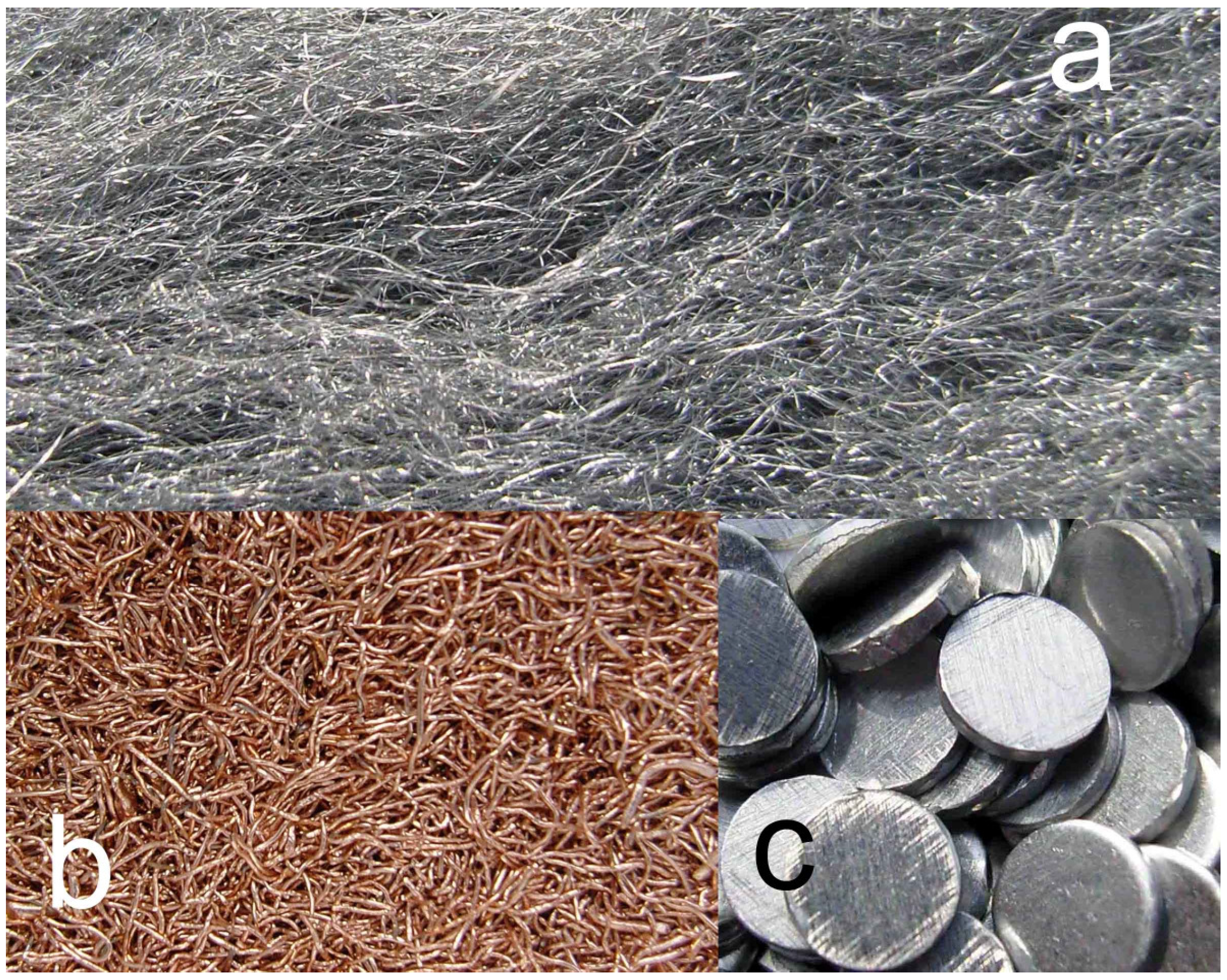
2.1.5. Materials and Methods

Measurements were made of EC, Eh, pH, and temperature using Hanna HI-98120 (ORP/Temperature, Hanna Calibration Number = 24,230), Hanna HI-98129 (pH, EC, TDS, Temperature; Hanna Calibration Number = 33,999). Hi-98120 is factory calibrated. HI-98129 was calibrated using Hanna test reagents (pH buffer solutions 4.01, 7.01, 10.01 (HI-7004, HI-7007, HI-7010) and conductivity solution 1.413 mS cm−1 (HI-7031)). Eh298.15K calculated from ORP [23,72] as:
Eh = ORP (298.15/To)
To = measured temperature, K.
TDS (Total dissolved solids, ppm) = EC (mS cm−1) × F × 103
F = a factor (e.g., 0.5) [72]. The untreated test water (pH = 6.2–7.1, Eh = 0.034–0.185 V) was extracted from an unconfined infiltration reservoir in fractured Devonian (Old Red Sandstone Volcanic Series, Ochil Hills, UK) basalts.

2.1.6. Borehole Reactor Structure: m-ZVM

Each prototype reactor tube contained a 3 m ZVM (0.04 m diameter) column. The ZVM was retained in place by ultra filtration membranes (0.1 m). The ZVM combination tested are BR1 (100% m-Fe0), BR2 (80 wt % m-Fe0 + 20 wt% m-Cu0), and BR3 (57 wt% m-Fe0 + 29 wt% m-Al0 + 14 wt% m-Cu0). Each reactor tube contained 0.4 kg m-Fe0. A maximum ΔP [1] of 15,000 Pa was applied. BR1-BR3 were operated using the same water source as MWR1-MWR5 and DR1-DR3. m-Fe0 = fine filaments (Figure 1); m-Al0 = 5 mm Al punchings (Figure 1); m-Cu0 = fine Cu filaments (0.0001–0.0005 m diameter, 0.001–0.005 m length (Figure 1)).

2.1.7. Static Diffusion Reactor Structure: m-ZVM

The micro-reactors (MWR1-MWR5) contain 0.0032 m3 H2O and tested five different ZVM combinations: MWR1: m-Fe0 (10 gm): MWR2: m-Fe0 (10 gm) + n-Fe0 (18 gm): MWR3: m-Fe0 (10 gm) + m-Cu0 (2.7 gm): MWR4: m-Fe0 (10 gm) + m-Al0 (2.8 gm): MWR5: m-Fe0(10 gm) + m-Al0 (2.8 gm) + mCu0(2.7 gm): n-Fe0 = powdered Fe, particle size <60,000 nm; m-Fe0 = fine filaments (0.0001–0.001 m diameter, 0.001–0.1 m length); m-Al0 = Al filings (0.0005–0.002 m) m-Cu0 = Cu filings (0.0005–0.003 m).

2.1.8. Continuous Flow Reactor Structure: n-ZVM

Each prototype reactor tube contained n-ZVM (Figure 2) in a 0.5 m vertical tube (0.04 m diameter) with a constant ΔP of 15,000 Pa. The n-ZVM had a particle size of <60,000 nm. The ZVM was retained in place by ultra filtration membranes (0.1 m). Each reactor tube contained a different n-ZVM column. DR1 = n-Fe0 (0.5 kg); DR2 = n-Fe0 (0.5 kg) + n-Cu0 (0.15 kg); DR3 = n-Fe0 (0.5 kg) + n-Cu0 (0.15 kg) + n-Al0 (0.13 kg).

2.2. Permeability of ZVM

The permeability of m-ZVM (Figure 1) and n-ZVM (Figure 2) was compared.

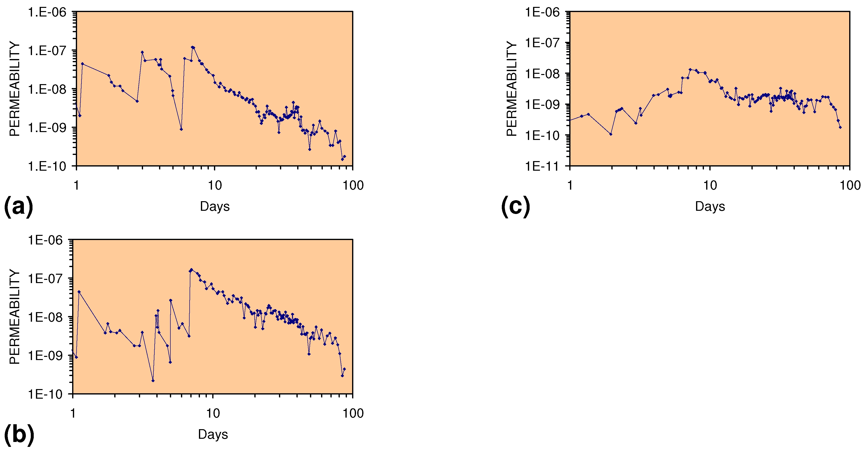
2.2.1. Permeability of n-ZVM

In DR1 and DR2 (Figure 3) permeability initially changed cyclically with abrupt increases being followed by a slow decline and subsequent abrupt rise. In each cycle, the permeability change is in the order of 102m3 m−2 s−1 Pa−1. This pattern is consistent with the cyclic change from viscous flow in unexpanded porosity to flow in expanded porosity (macropore/fluidised flow/piping flow) followed by a gradual collapse of the expanded porosity (e.g., macropore collapse) [1,2,29,30,31]. This type of poro-elastic flow occurs in clayey and sandy sequences [1,29]. After around 7–8 days, the cyclic flow pattern ceases and the flow shows a general logarithmic decline with minor fluctuations. This change is associated with two changes in the n-ZVM bed:
  • The n-ZVM becomes increasingly consolidated due to Fe-oxide formation and Fe particle growth
  • O2 gas bubbles start to discharge from the n-ZVM bed as the permeability reduces. This results in pore throat occlusion with an associated decrease in permeability [1].
Initial permeability in DR3 (Figure 3) is substantially lower than in DR1 and DR2, and remains constant with time at around 10−9 m3 m−2 s−1 Pa−1. The lower permeability is associated with extensive O2(g) venting from the n-ZVM bed shortly after formation.
Figure 3. Change in n-ZVM permeability with time. (a) DR1, (b) DR2, (c) DR3: ΔP = 15,000 Pa.
Sustainability 02 02988 g003

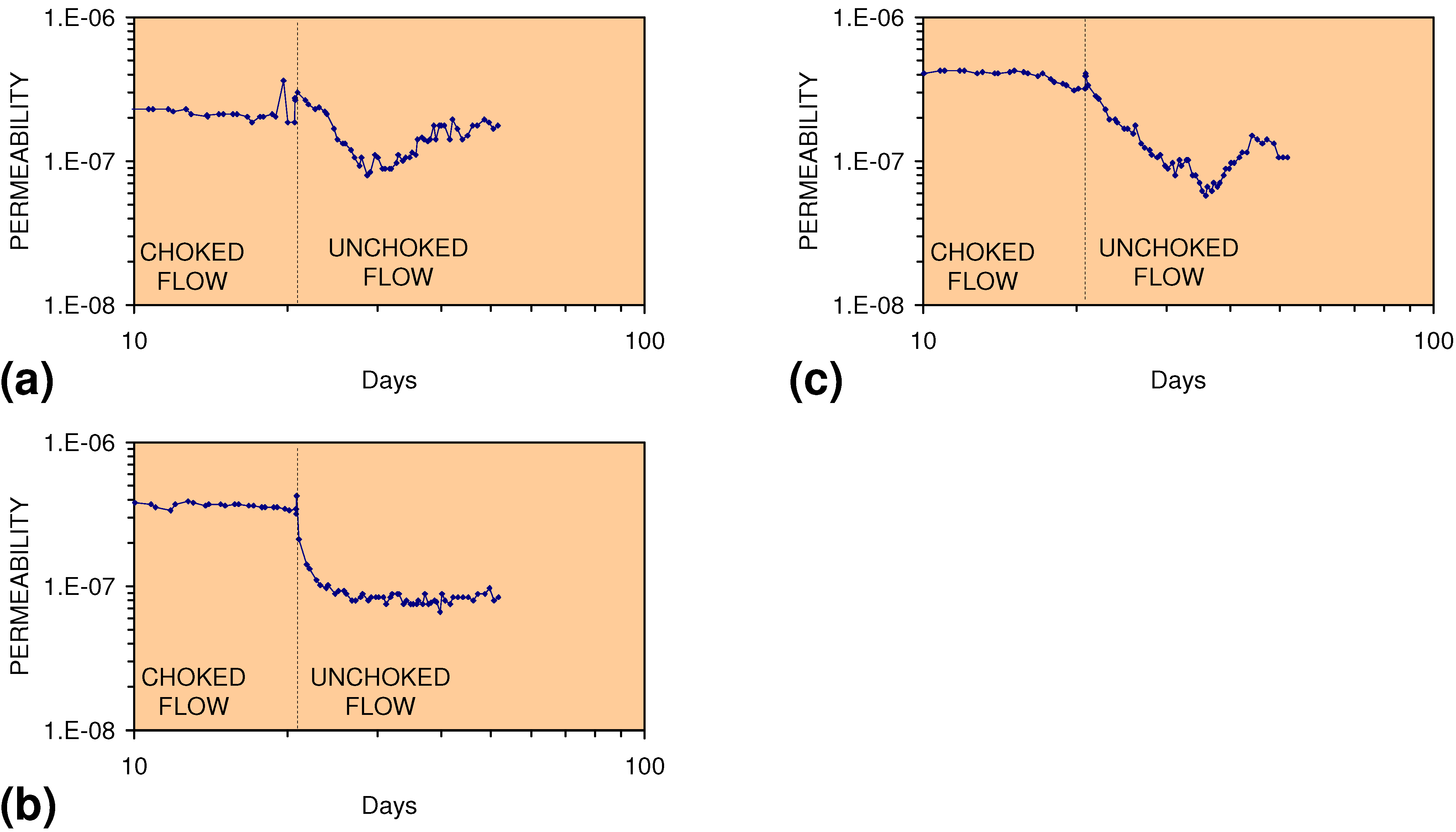
2.2.2. Permeability of m-ZVM

The permeability of m-ZVM (Figure 4) is about 102 m3 m−2 s−1 Pa−1 higher than the permeability in an equivalent n-ZVM bed (Figure 3). Discharge from each borehole reactor was controlled by a valve. The valve aperture was operated in two positions. (i) choked flow, where the discharge aperture was reduced by 50%, and (ii) unchoked flow where the valve aperture was not restricted. The n-ZVM reactors (Figure 3) were operated with unchoked flow. m-ZVM operated under choked flows is able to maintain a constant permeability (Figure 4). However, when the flow are unchoked, the permeability varies with time around an average permeability of 10−6 to 10−7 m3 m−2 s−1 Pa−1. The reactors were switched off when the m-ZVM ceased to alter the Eh and pH of the water flowing through the reactor.
Figure 4. Change in m-ZVM permeability with time. (a) BR1, (b) BR2, (c) BR3: ΔP = 15,000 Pa.
Sustainability 02 02988 g004

2.2.3. Significance of Permeability Observations

The n-ZVM and m-ZVM permeability observations (Figure 3 and Figure 4) indicate that about 100 times more n-ZVM (than m-ZVM) will be required to treat/process a specific water flow rate. This indicates that replacement of n-ZVM with m-ZVM will have the following advantages:
  • The size of the facility required to process a specific water flow rate is reduced by a factor of 100
  • The weight of ZVM required to process a specific water flow rate is reduced by a factor of 100
  • The volume of water which can be processed/unit time by a specific weight of ZVM is increased by a factor of 100.
The effectiveness of a water treatment can be defined by the proportion of a component removed from a specific volume or flow rate of water. The economics of a treatment facility is based on the cost per unit volume of water per unit volume of ZVM. The permeability analysis demonstrates that significantly less m-ZVM is required to process a specific volume of water. The experimental analyses in the next sections demonstrate that this smaller quantity of m-ZVM can provide both a more effective and more focused nitrate, metal and organic chemical treatment for flowing water and recirculating water than the substantially larger volume of n-ZVM. m-ZVM treatment is demonstrated to remove <60–100% of the contaminant. It is able to achieve this treatment without a significant increase in pH. The large increases in treated water pH associated with n-ZVM can render the product water unfit for human consumption [5]. This study demonstrates that the minor changes in pH (typically < 1) associated with m-ZVM treatment allow the treated product water to be used for human consumption. This study also demonstrates that higher levels of nitrate removal occur at high space velocities than low space velocities. This observation renders m-ZVM a more effective (and more economic) nitrate treatment medium for flowing water than the lower permeability n-ZVM.
Most n-ZVM is manufactured as graded particles which may be coated with one or more of metal and other chemicals [6]. The n-ZVM is commonly mixed with water and other chemicals to form a slurry which can be injected into the sediment [6]. The water (containing n-ZVM) migrates radially during injection through the macropores and fractures from the injection point through the aquifer [1,2]. Following injection, the n-ZVM settles and accumulates within the macropores, fractures and pores as the driving force is removed [1]. The macropore/fracture permeability associated with injection decreases with increasing distance from the injection point [1]. This results in a radial settling of the n-ZVI around the injection point. The distribution of n-ZVI within the aquifer can be directly linked to the permeability and injection pressure. Injection of n-ZVM slurry can result in clogging of pores [6,21] and a substantive drop in permeability by several orders of magnitude [6]. Increases in driving force (injection pressure) may be required to re-establish the original permeability [1,2,29,30]. In addition to this clogging, recrystallisation of the n-ZVM can result (over a period of time) in a decrease in aquifer permeability of several orders of magnitude [15].
Equation 6 indicates that n-ZVM (Figure 2) will have a lower permeability than m-ZVM (Figure 1) because it is nano grade (and has a lower pore throat radii). The experimental tests show that fresh n-ZVM (Figure 3) can have a similar permeability to fresh m-ZVM (Figure 4). Fresh n-ZVM is able to achieve a similar permeability to fresh m-ZVM, because the smaller particles allow low tortuosity, high permeability macropore conduits to form as the n-ZVM porosity expands and contracts in response to the applied driving force [1,2,29,30].

2.3. Impact of O2(g) Generation by ZVM on GWM Permeability

ZVM produces O2 (from the reduction of water) as a by-product of the interaction of Fe and cations/anions. While the chemistry associated with the O2 production is complex and poorly understood [22,24,25,38], the commercial implications of the O2 production in water treatment are assessed here by examining the sedimentological/hydrodynamic features associated with O2 production in a number of static diffusion reactors containing n-ZVM and n-ZVM + Ca-montmorillonite (clay).

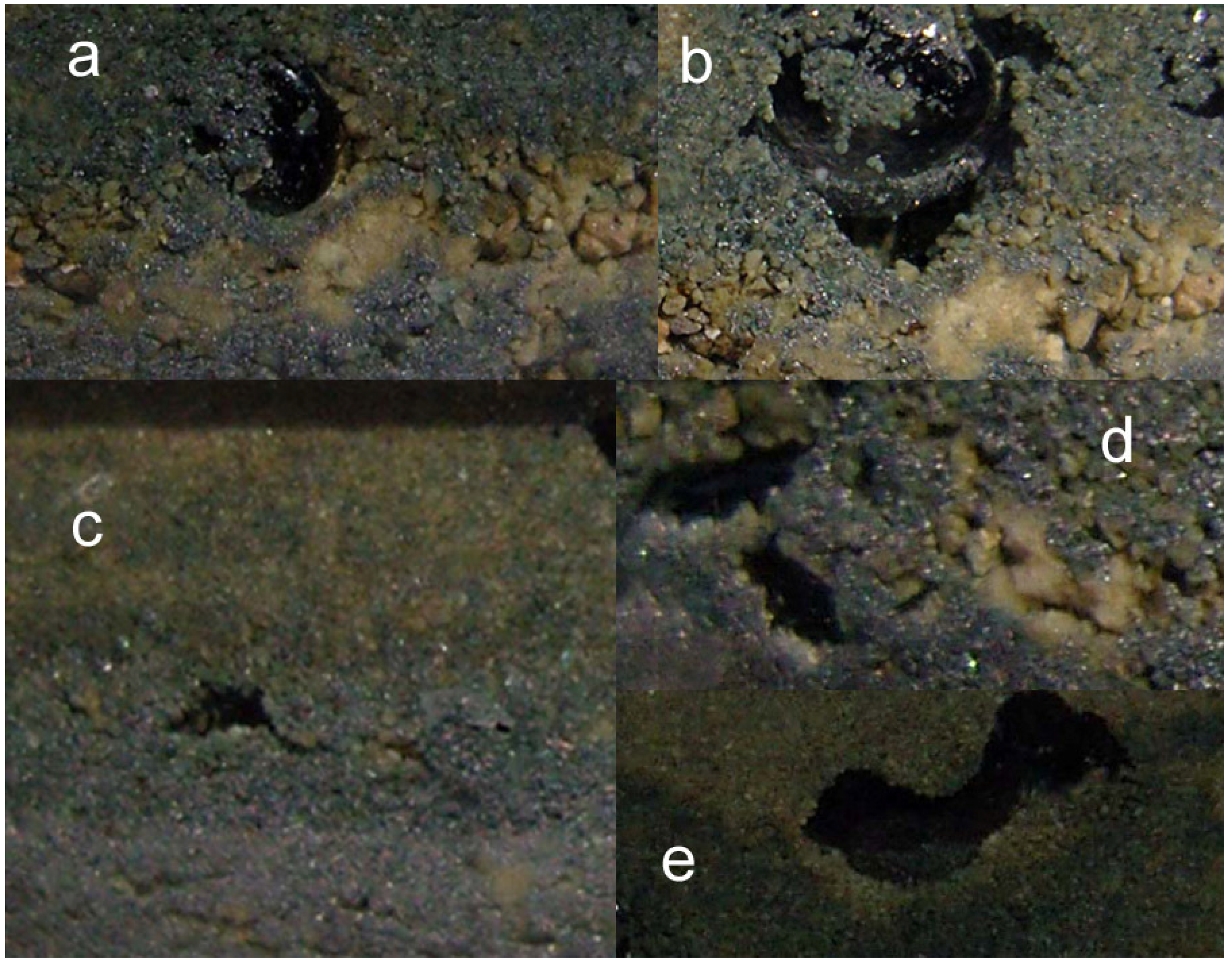
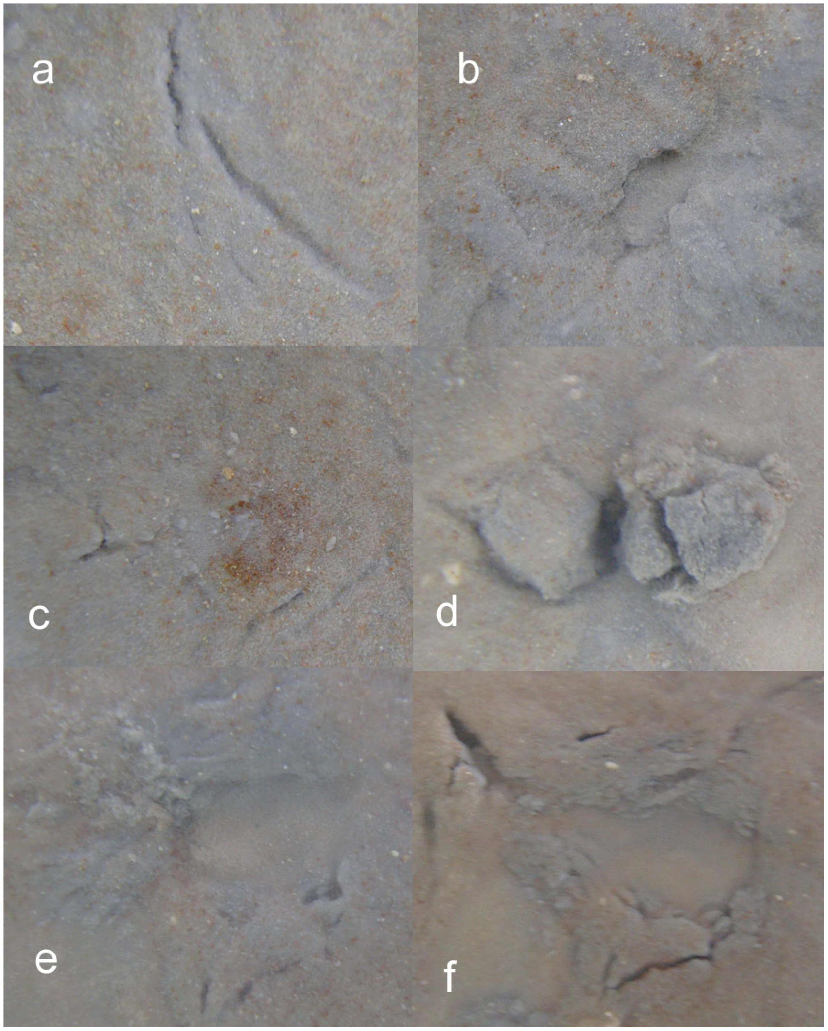
2.3.1. Creation of Macropores Associated with O2 generation

In a self-sealing GWM air bubble migration is associated with accumulation of air in vugs, which are fed by feeder macropores [1]. The buoyant pressure associated with the air accumulation resulted in growth of the vugs [1]. The increased vug volume fills with water [1]. Some of the water in the vug discharges with the air when it eventually escapes [1]. Exactly the same pattern of vug formation occurs in a n-ZVM bed. In a self-sealing GWM, the presence of air bubbles switches the water flow mechanism from viscous flow to the Knudsen diffusion rate for air [1,2]. This has the impact of reducing the permeability of the pore network by a factor of about 10−6 [1]. However, once the air bubble has been discharged, the relict pore network has a high permeability which may be in the order of 10−5m3 m−2 s−1 Pa−1 [1,2,29,30].
n-ZVM containing n-Al0 and n-Fe0 is characterized by the substantial early discharge of O2, while the volume of O2 discharged increases with time for n-Fe0 and n-Fe0 + nCu0. The rate of O2 discharge is a major factor controlling the permeability of n-ZVM (Figure 3).
The presence of clays alters the permeability associated with n-ZVM. This is illustrated for a sediment bed comprising n-Fe0—Ca-montmorillonite (clay). In this type of sediment bed, O2 bubbles are fed by a network of macropores (Figure 5). The macropores are separated by clay clods (Figure 5). Bouyant pressure forces the bubbles to rise with time (Figure 5). This movement results in the vug enlarging with time. The bubble may change from a spherical form (Figure 5a) to an ellipsoid (Figure 5b). In the example illustrated in Figure 5b, the base of the initial vug remains adhered to the bubble. The resulting sediment separation creates a water filled vug below the O2 bubble. Following discharge of the O2, the vugs and their feeder macropores remain open (Figure 5c, d, e). These relict macropores increase the permeability and storage capacity of the clay. The O2 venting results in a gravity segregation of the sediment bed, with the clay concentration increasing towards the sediment-water contact (Figure 5c, e). The macropores and vugs are concentrated in the sections of the sediment bed, which contain a high n-Fe0 concentration (Figure 5d). Vugs in the clay rich section may contain accumulations of heavier n-Fe0 (Figure 5e). The permeability of the clay rich layers is low (Figure 5c). However, the O2 venting results in the formation of cracks/fissures, which extend to the sediment surface from the feeder vug (Figure 6). The presence of feeder vugs results in the presence of static craters on the sediment surface which are continually reused by discharging O2 (Figure 6).
The development of vents, fissures and macropores in a bed containing n-Fe0 and smectite (montmorillonite) clay indicates that n-Fe0 (or addition of Fe(a−n)+ ions) could be used to increase and expand the macropore network (and storage capacity) of the clay within the aquifer/GWM/plume.
Figure 5. Cross Section of a n-Fe0—Ca-montmorillonite (clay) bed in fresh water showing O2 bubbles being fed by water filled macropore porosity separating clay clods within Ca-montmorillonite rich layers. (a) 16 days after n-ZVM bed formation. Large O2 bubble diameter = 3 mm. Eh = −0.134 V; pH = 8.59; EC = 0.816 mS cm−1; Temperature, T = 21 °C; ZVM bed weight ratio 1.2 Ca-montmorillonite: 1 n-Fe0. (b) 21 days after n-ZVM bed formation. The vug has grown over the preceding 5 days due the buoyant pressure created by the O2 bubble and the feeder macropore network has become more pronounced. O2 bubble diameter = 3 mm; Eh = −0.171 V; pH = 8.55; EC = 0.791 mS cm−1; T = 13.8 °C; (c) Cross section through n-ZVM + clay bed from the sediment-water contact. The bed shows density stratification with clay concentrations increasing towards the sediment-water contact. The n-Fe0 rich layers are characterized by the presence of vugs (formed by O2 bubbles). Vertical section = 10 mm. (d) Cross section showing water filled vugs fed by a macropore network (following O2 discharge) separated by clay clods. Vug diameter = 2 mm. (e) Cross section through graded n-ZVM + clay bed showing water filled vugs following discharge of O2. The larger vug contains a relict layer of settled n-Fe0, which has settled following the discharge of the O2 bubble, which formed the vug. Field of view = 10 mm. Photographs b–e taken 21 days after n-ZVM bed formation. Water composition prior to addition of n-ZVM: Eh = 0.152 V; pH = 6.39; EC = 0.261 mS cm−1.
Sustainability 02 02988 g005
Figure 6. Cracks, fissures and vents associated with O2 discharge from a Ca-montmorillonite – n-Fe0 bed in saline water. (a) Individual fractures contain macropores leading to deeper O2 filled vugs. Field of view = 20 mm. 8 days after n-ZVM bed formation. Eh = −0.006 V; pH = 8.62; EC = 2.149 mS cm−1; T = 14 °C; (b) Collapsed O2 discharge vent (5 mm diameter). 10 days after formation of the n-ZVM bed. Eh = 0.031 V; pH = 8.50; EC = 2.030 mS cm−1; T = 14.1 °C; (c) Collapsed O2 discharge vent and associated venting cracks. 10 days after formation of the n-ZVM bed. 3 cm field of view. (d) Active O2 discharge vent. Field of view = 20 mm. 21 days after n-ZVM bed formation. Eh = 0.042 V; pH = 8.43; EC = 2.030 mS cm−1; T = 25.1 °C; (e) Active O2 discharge vent (illustrated in Figure 6b) just prior to discharge. Field of view = 20 mm. 21 days after n-ZVM bed formation. (f) Active O2 discharge vent (illustrated in Figure 6e) immediately after discharge. Field of view = 20 mm. 21 days after n-ZVM bed formation. Water composition prior to addition of n-ZVM: Eh = 0.147 V; pH = 6.27; EC = 1.836 mS cm−1; ZVM bed weight ratio 1.2 Ca-montmorillonite: 1 n-Fe0.
Sustainability 02 02988 g006
Figure 7. n-Fe0 and n-Fe0 + n-Cu0: Fresh water. (a) Cracks through a limonite crust revealing the underling n-Fe0 at the n-ZVM- water interface. The cracks are associated with O2 discharge. 95 days after formation of n-Fe0 bed. Field of view = 30 mm. Eh = 0.012 V; pH = 8.27; EC = 0.308 mS cm−1; T = 15.3 °C; Water composition prior to addition of n-ZVM: Eh = 0.043 V; pH = 6.90; EC = 0.426 mS cm−1; (b) Cracked section of limonite crust being lifted by an underlying O2 bubble 95 days after formation of n-Fe0 bed. O2 bubble diameter = 7 mm. (c) n-Fe0 + n-Cu0 clods (separated by macropores) containing limonite patches (yellow). Field of view = 5 mm. 91 days after n-ZVM bed formation. Eh = −0.012 V; pH = 8.97; EC = 0.228 mS cm−1; T = 13.9 °C; Water composition prior to addition of n-ZVM: Eh = 0.032 V; pH = 7.10; EC = 0.347 mS cm−1; (d) n-Fe0 + n-Cu0 clods separated by macropores. O2(g) is discharged through the macropores beside the limonite patches. Field of view = 5 mm. 91 days after formation of n-ZVM bed. (e) n-Fe0 + n-Cu0 clods located beside inactive macropores. Field of view = 5 mm. 91 days after formation of n-ZVM bed. ZVM bed weight ratio: 6.5 n-Fe0:1 n-Cu0.
Sustainability 02 02988 g007
Figure 8. n-Fe0 + n-Al0 + n-Cu0 (saline pore water). (a) Cross section view through the n-ZVM water surface: n-Cu0 diapir on n-Fe0 + n-Al0 surface. Large diapir diameter = 4 mm. O2(g) degassing from smaller n-Cu0 diapirs and directly from the n-Fe0-n-Al0 bed. The underlying n-ZVM bed is laminated and a series of nodular (Fe) concretions are developing. 10 days after the formation of the n-ZVM bed. (b) Plan view: n-Cu0 diapir on n-Fe0 + n-Al0 surface. Diapir diameter = 4 mm. 10 days after the formation of the n-ZVM bed. Eh = −0.115 V; pH = 9.25; EC = 2.260 mS cm−1; T = 14.1 °C; (c) Central cone starting to reveal an O2 bubble. Diapir diameter = 5 mm. (d) Plan view of active O2(g) discharge creating cratered cones of n-Cu0 on an n-Fe0 surface at the n-ZVM-water interface. 7 days after n-ZVM bed formation. The largest crater (Figure 8e) has an O2(g) bubble diameter of 7 mm. Eh = −0.056 V; pH = 9.51; EC = 2.256 mS cm−1; T = 14.1 °C; (e) Cross section through n-ZVM bed illustrating a cone on the n-ZVM-water interface. (f) Cross-section through the n-ZVM bed showing an oxygen bubble emerging from a n-Cu0 cone. Diapir diameter = 3 mm. 10 days after the formation of the n-ZVM bed. Saline water composition prior to addition of n-ZVM: Eh = 0.147 V; pH = 6.27; EC = 1.836 mS cm−1. ZVM bed weight ratio: 6.5 n-Fe0:1.67 n-Al0: 1 n-Cu0.
Sustainability 02 02988 g008

2.3.2. n-Fe0 and n-Fe0 + n-Cu0

Clay free n-ZVM beds composed of n-Fe0 tend not to show vents or extensive macropores. The sediment-water contact may form an oxidized crust of limonite/goethite (Figure 7). This crust becomes fractured, exposing the underlying n-Fe0 (Figure 7). The development of the cracks/fissures/fractures is associated with the gathering and discharge of O2(g) (Figure 7).
The addition of n-Cu0 to n-Fe0 substantially reduces the amount of limonite at the sediment-water interface (Figure 7). The sediment water interface comprises clods separated by macropores (Figure 7). Limonite patches on the sides of some of the clods (Figure 7) are associated with active O2(g) venting (Figure 7).

2.3.3. n-Fe0 + n-Al0 + n-Cu0

Mixtures of n-Al0 + n-Cu0 + n-Fe0 (and n-Al0 + n-Fe0) are associated initially with active O2(g) degassing with associated discharge of n-Al0 + n-Cu0 + n-Fe0 into the overlying water column (Figure 8) . This results in the formation of active n-Cu0 cones (Figure 8) and the active suspension of n-ZVM in the water column. The degassing of O2 to the air-water contact results in flotation of n-Cu0 on the water surface (Figure 9). The rate of O2 degassing decreases with time.
O2 bubbles initially originate in layers containing n-Cu0. This results in the formation on the sediment-water surface of cones of n-Cu0 (Figure 8 and Figure 9). These cones form around O2 bubbles (Figure 8 and Figure 9). Following O2 release the vents collapse leaving a small pockmark and ejected n-ZVM around the discharge point (Figure 9). Clods separated by macropores discharging O2 from the n-Fe0/n-Al0 surface develop around the discharge crater (Figure 9). Over time these macropores (separated by clods) become the dominant discharge routes for O2 (Figure 9). The clods give the n-ZVM-water surface a particulate appearance (Figure 9). The clods are not particles but form an irregular sediment interface with the water (Figure 10).

2.3.4. Significance of O2

O2 discharge reduces the permeability of an n-ZVM bed by pore occlusion (Figure 3). This discharge creates a network of macropores within the n-ZVM bed and results in a continual discharge of fluid from the n-ZVM bed into the overlying water (Figure 5, Figure 6, Figure 7, Figure 8, Figure 9 and Figure 10). The fluid discharge controls the Eh and pH of the aquifer.
Figure 9. n-Fe0 + n-Al0 + n-Cu0. ZVM bed weight ratio: 6.5 n-Fe0: 1.67 n-Al0: 1 n-Cu0. (a) Plan view: n-Cu0 diapers on n-Fe0 + n-Al0 surface. The central cones contain O2 bubbles. Large diapir diameter = 4 mm. n-Fe0 + n-Al0 surface shows macropores associated with O2 venting starting to develop. 8 days after n-ZVM bed formation. Eh = −0.060 V; pH = 9.52; EC = 2.231 mS cm−1; T = 12 °C; (b) Collapsed n-Cu0 cone following venting. Note the O2 bubbles associated with clods around the edge of the ejecta from the collapsed cone. Field of view = 15 mm. 8 days after n-ZVM bed formation. (c) Active n-Cu0 cone. Note the O2 bubble has a larger diameter than the cone and is fed through a small crater within the cone. A circular zone of clods separated by macropores (discharging O2) has developed around the cone. O2 Bubble Diameter = 3 mm. 8 days after n-ZVM bed formation. (d) Vented n-Cu0 on the surface of the water. 10 days after the formation of the n-ZVM bed. (e) Clods separated by macropores (with O2 discharge) 10 days after n-ZVM formation. Field of view = 5 mm. Eh = −0.115 V; pH = 9.25; EC = 2.260 mS cm−1. (f) clods separated by macropores (with O2 discharge) 16 days after n-ZVM formation). Field of view = 10 mm. Eh = −0.091 V; pH = 9.24; EC = 2.190 mS cm−1; T = 18.4 °C; (g) well developed clods separated by macropores (with O2 discharge) (after 110 days following n-ZVM formation). Field of view = 20 mm. Eh = −0.161 V; pH = 8.48; EC = 0.19 mS cm−1; T = 18.5 °C; (Freshwater Feed: Eh = 0.032 V; pH = 7.12; EC = 0.347 mS cm−1). Figure 9a–f are in saline water feed Eh = 0.147 V; pH = 6.27; EC = 1.836 mS cm−1.
Sustainability 02 02988 g009
Figure 10. Cross section through the n-ZVM bed (n-Fe0 + n-Al0 + n-Cu0 (saline pore water)) showing lamination, n-Al0 diapirism and an irregular water-n-ZVM contact associated with the formation of clods. 16 days after n-ZVM formation. Field of view = 30 mm. The irregular n-ZVM water surface forms the clods (Figure 9). ZVM bed weight ratio: 6.5 n-Fe0:1.67 n-Al0:1 n-Cu0. Eh = −0.091 V; pH = 9.24; EC = 2.190 mS cm−1.
Sustainability 02 02988 g010

3. Results

3.1. Static Diffusion Reactor Results

The changes in redox environment form a series of regression relationships. These relationships allow prediction of the Eh and pH of the water surrounding an infiltration device, borehole or well containing m-ZVM as a function of time. Specific features are:
  • pH increases with decreasing SV to a maximum pH before subsequently declining (Figure 11)
  • Eh initially declines with decreasing SV, before subsequently increasing (Figure 12)
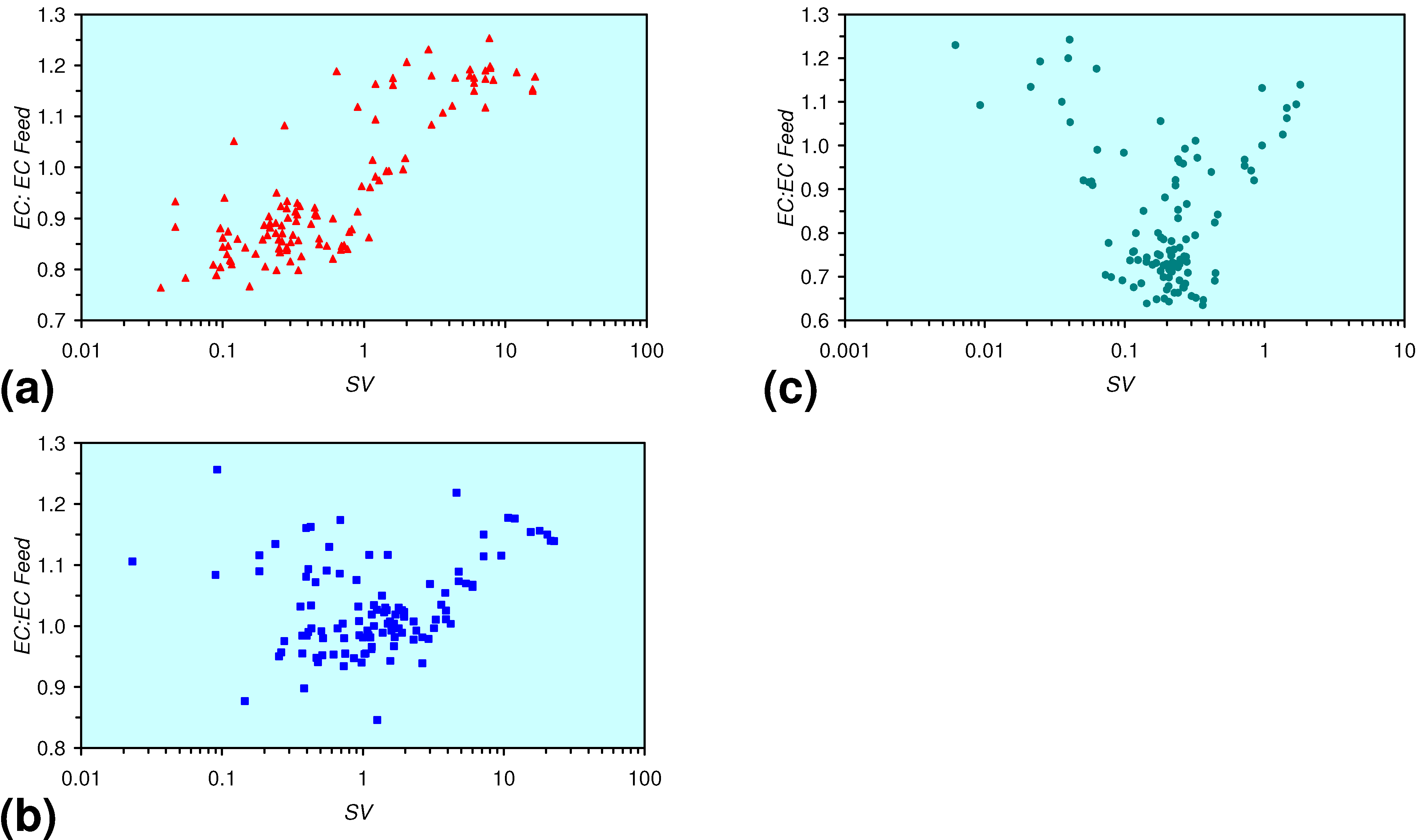
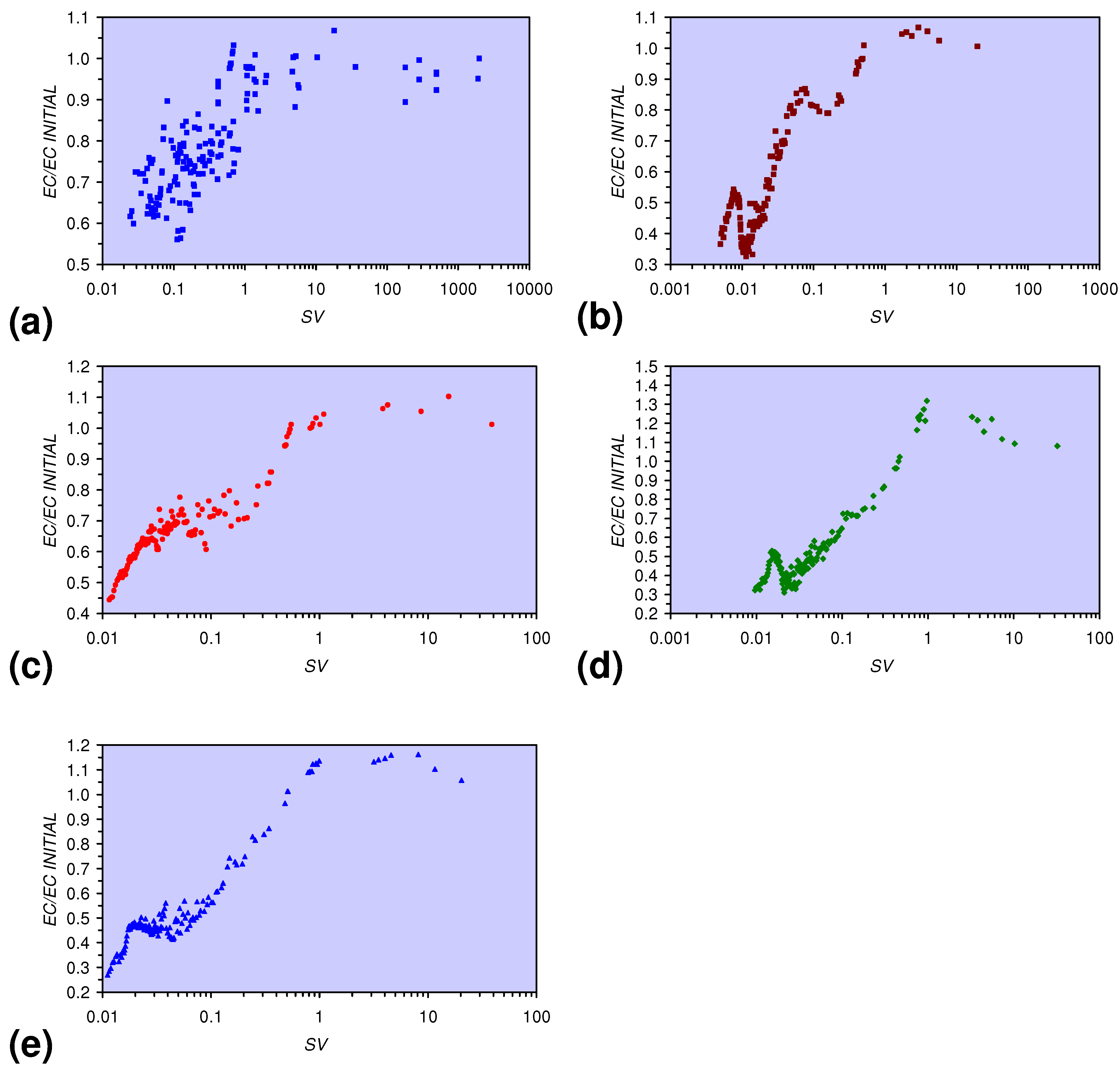
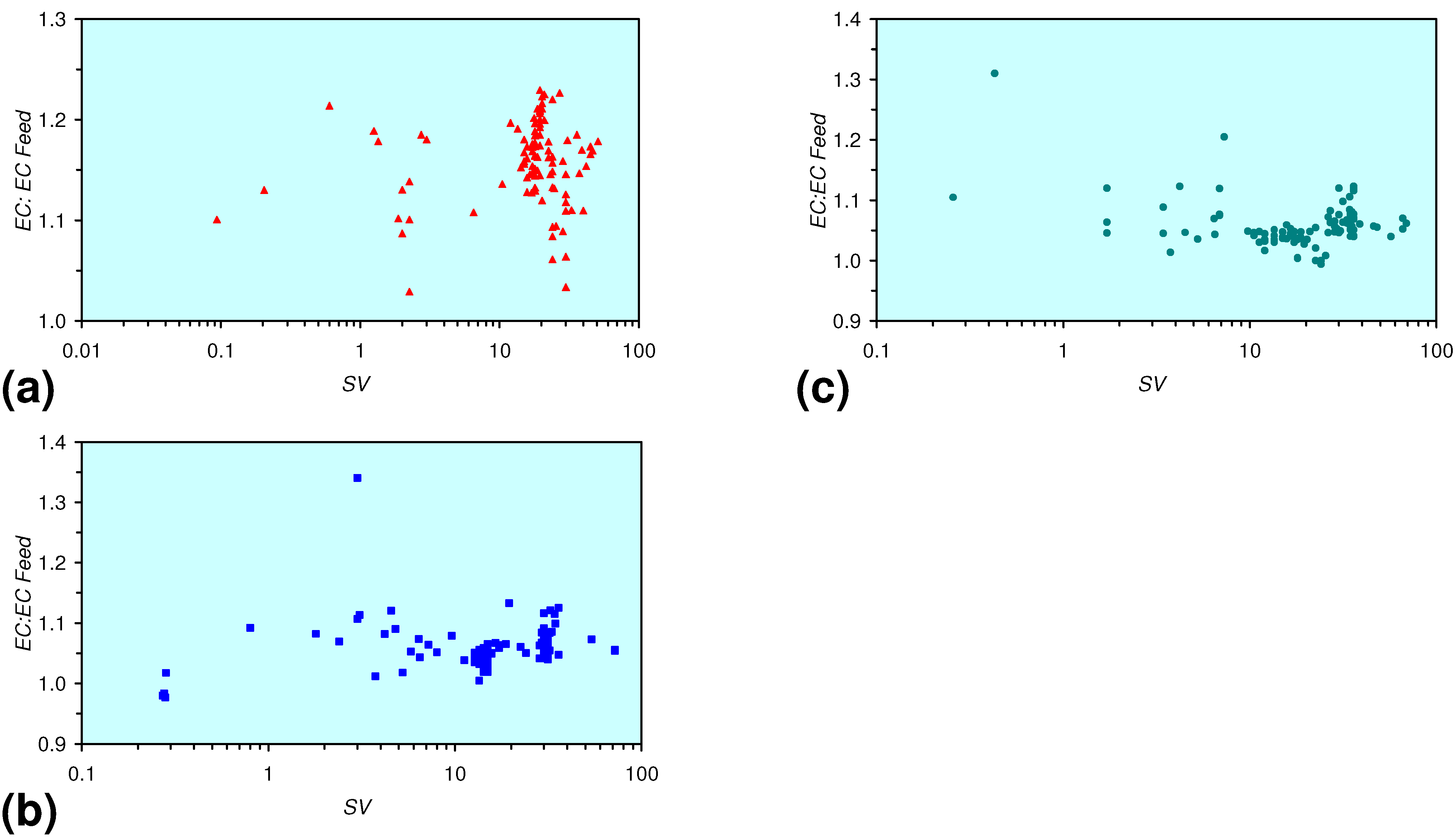
  • The EC:EC Initial ratio initially rises with decreasing SV, before subsequently reducing. The ratio may reduce to <30% (Figure 13), indicating that m-ZVM can be an effective remover of dissolved ions within water.
  • Eh vs. pH relationships demonstrate (Figure 14) that initially as SV decreases the redox environment moves to the NH4+: NOx (N2(aq)) redox fence [73]. Subsequent reductions in SV move the redox environment into the Fe2O3 stability zone [73].
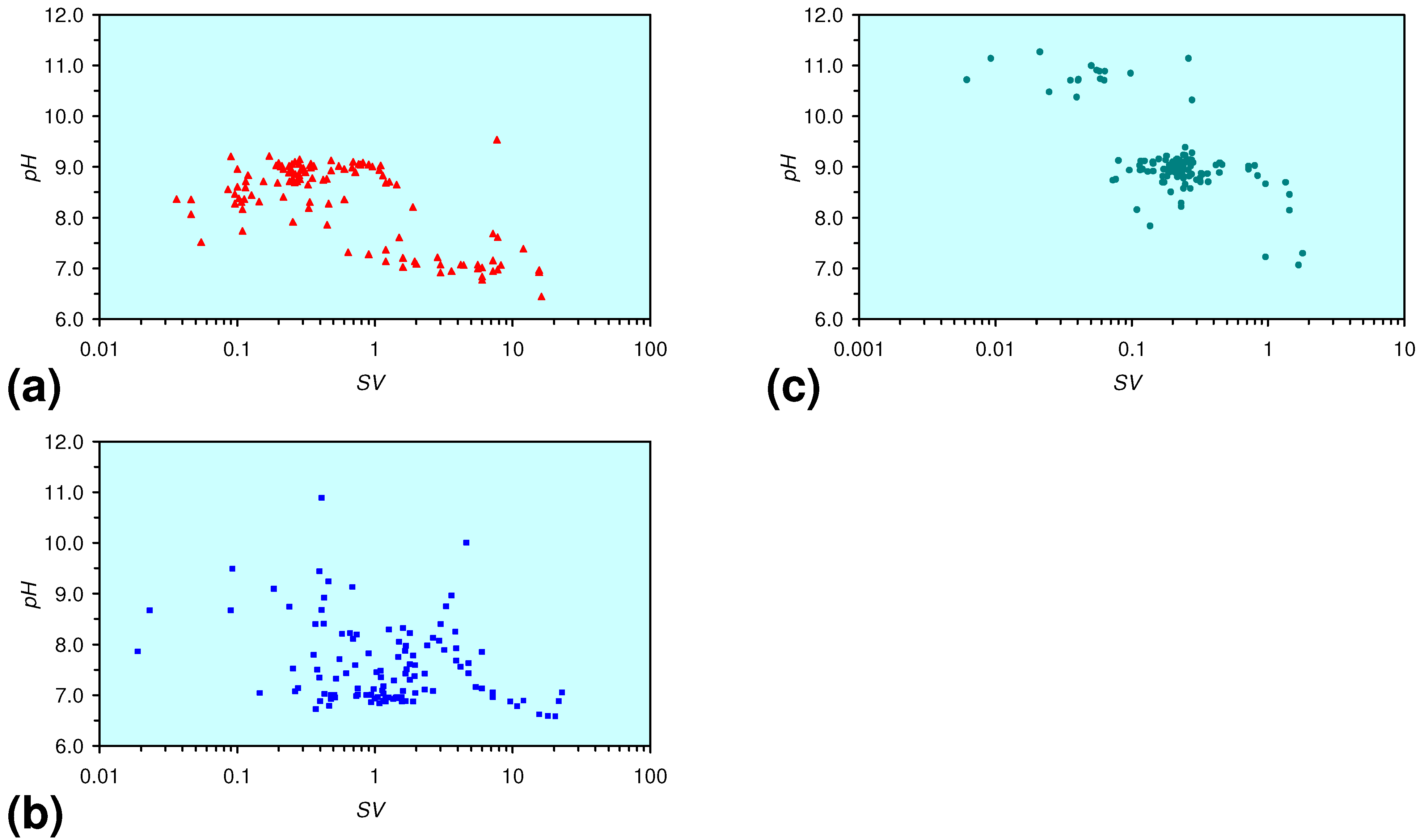
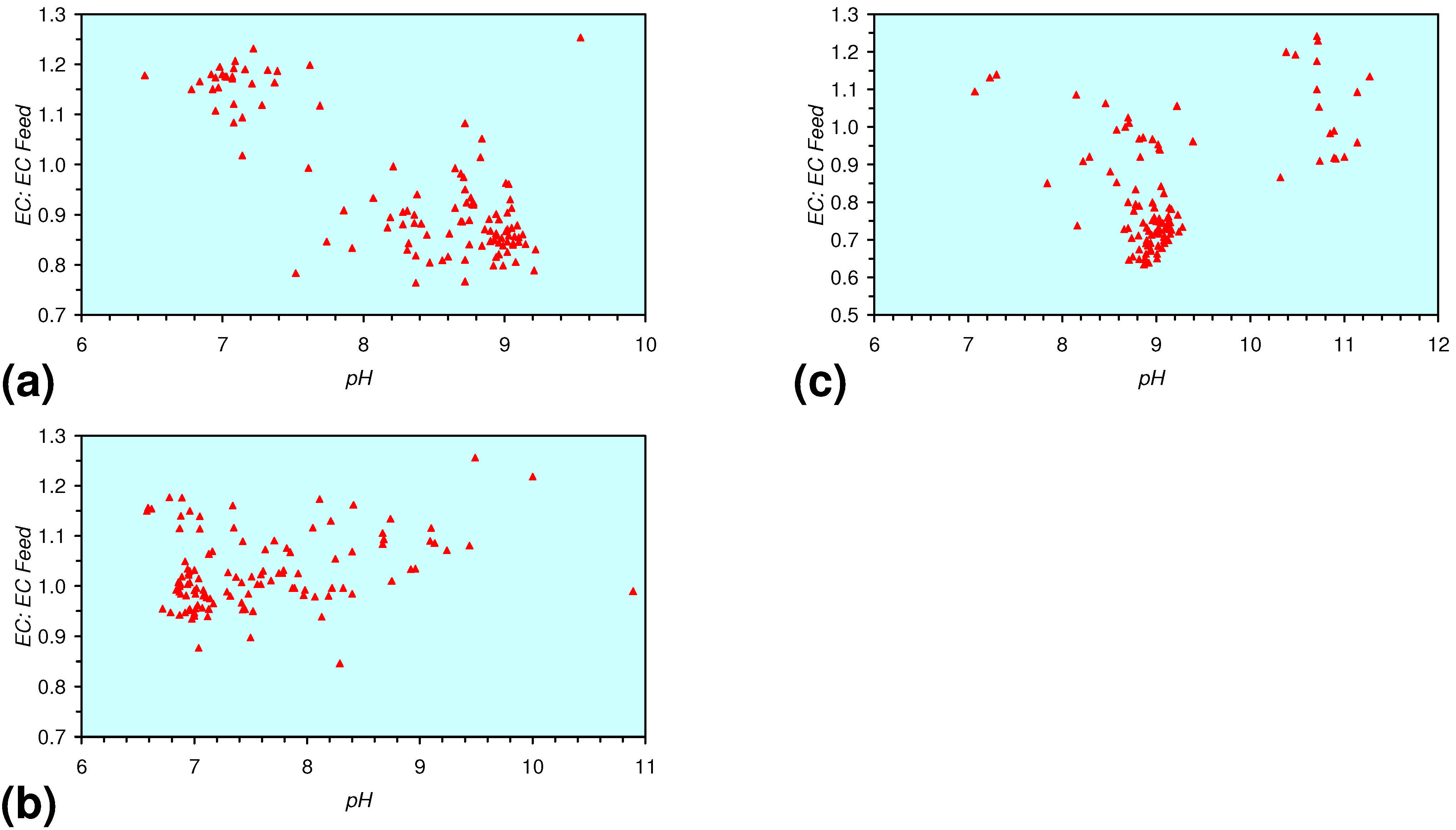
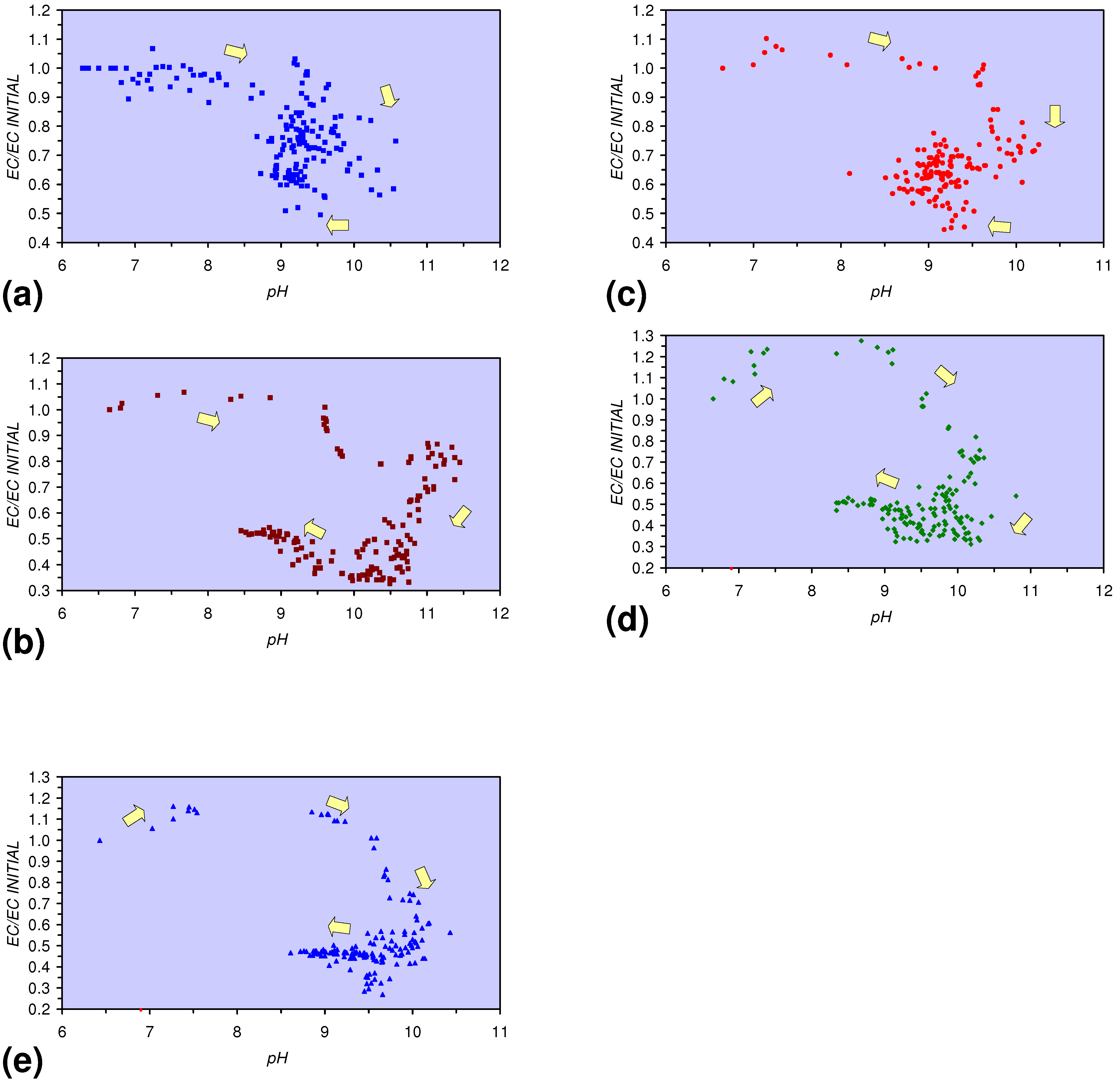
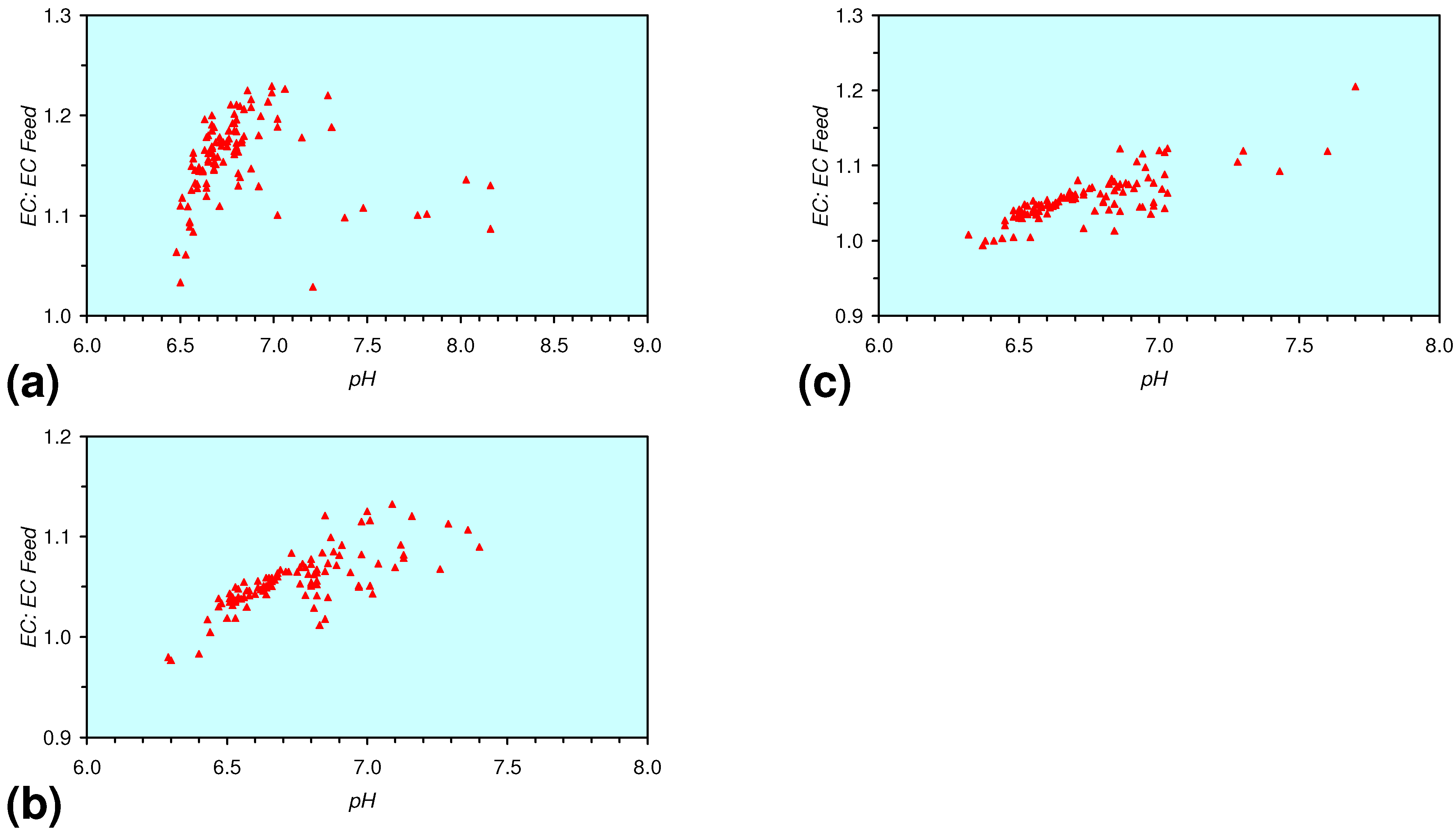
  • The EC:EC Initial ratio initially rises with increasing pH but decreases as the pH declines with decreasing SV (Figure 15).
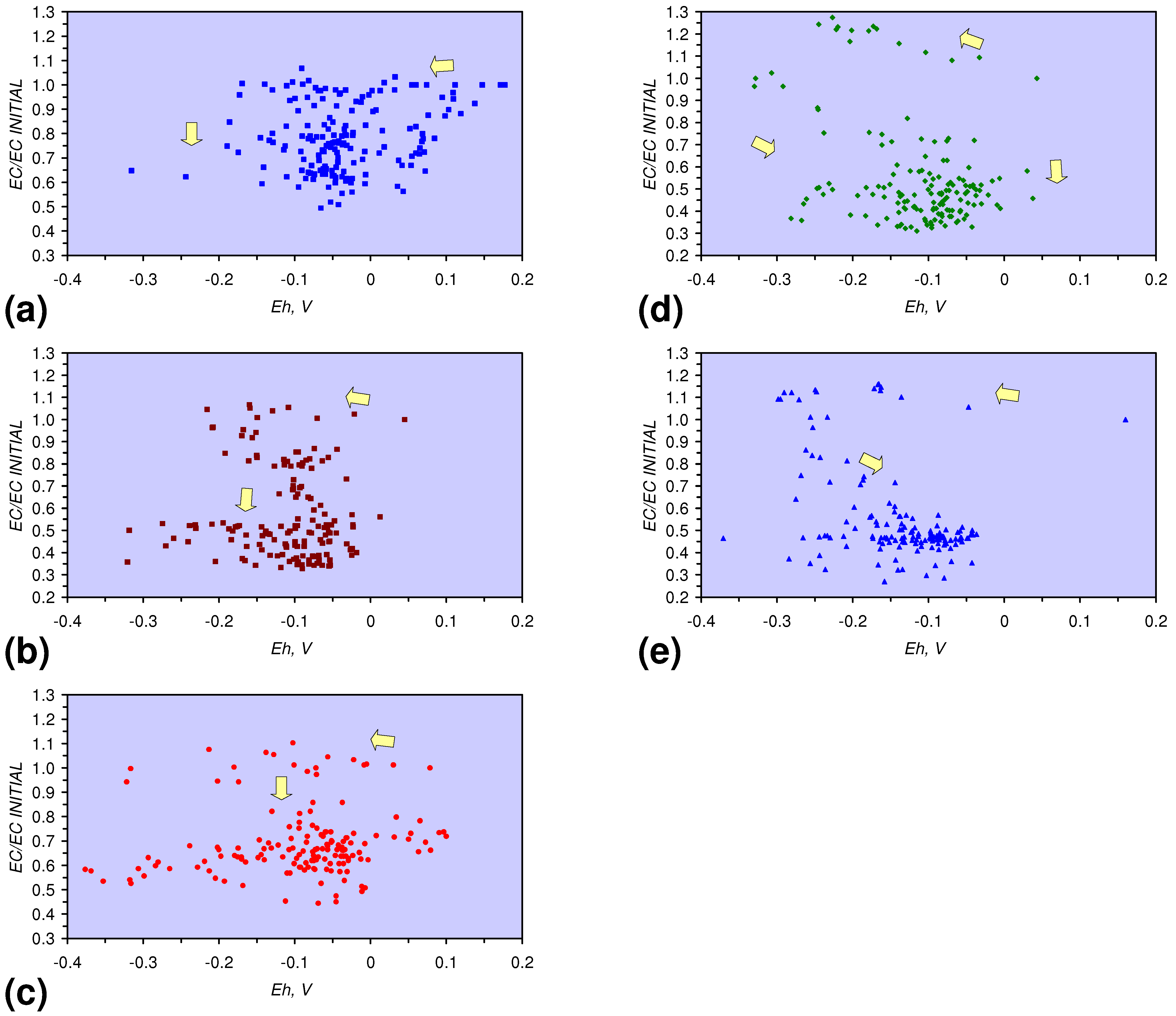
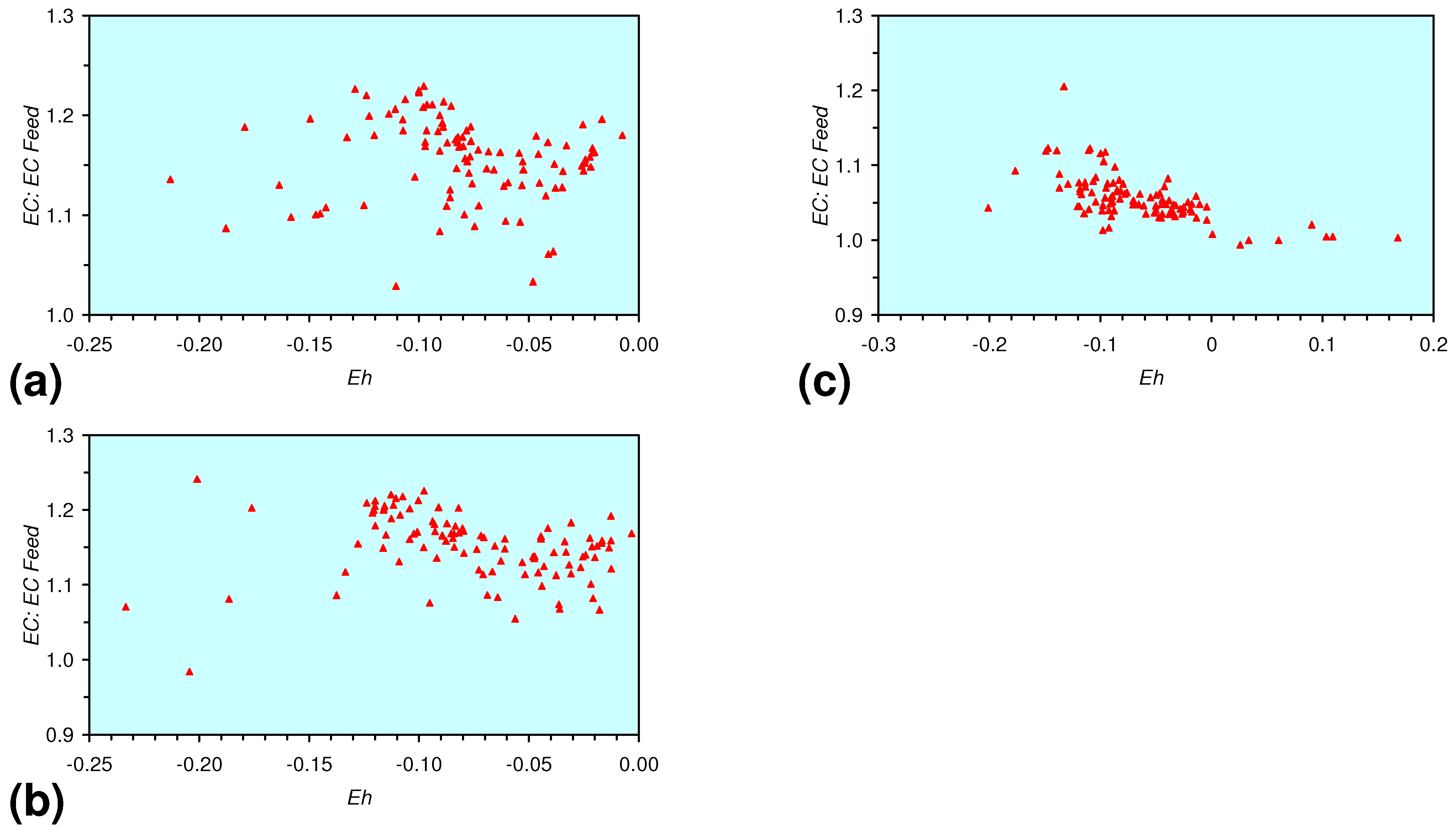
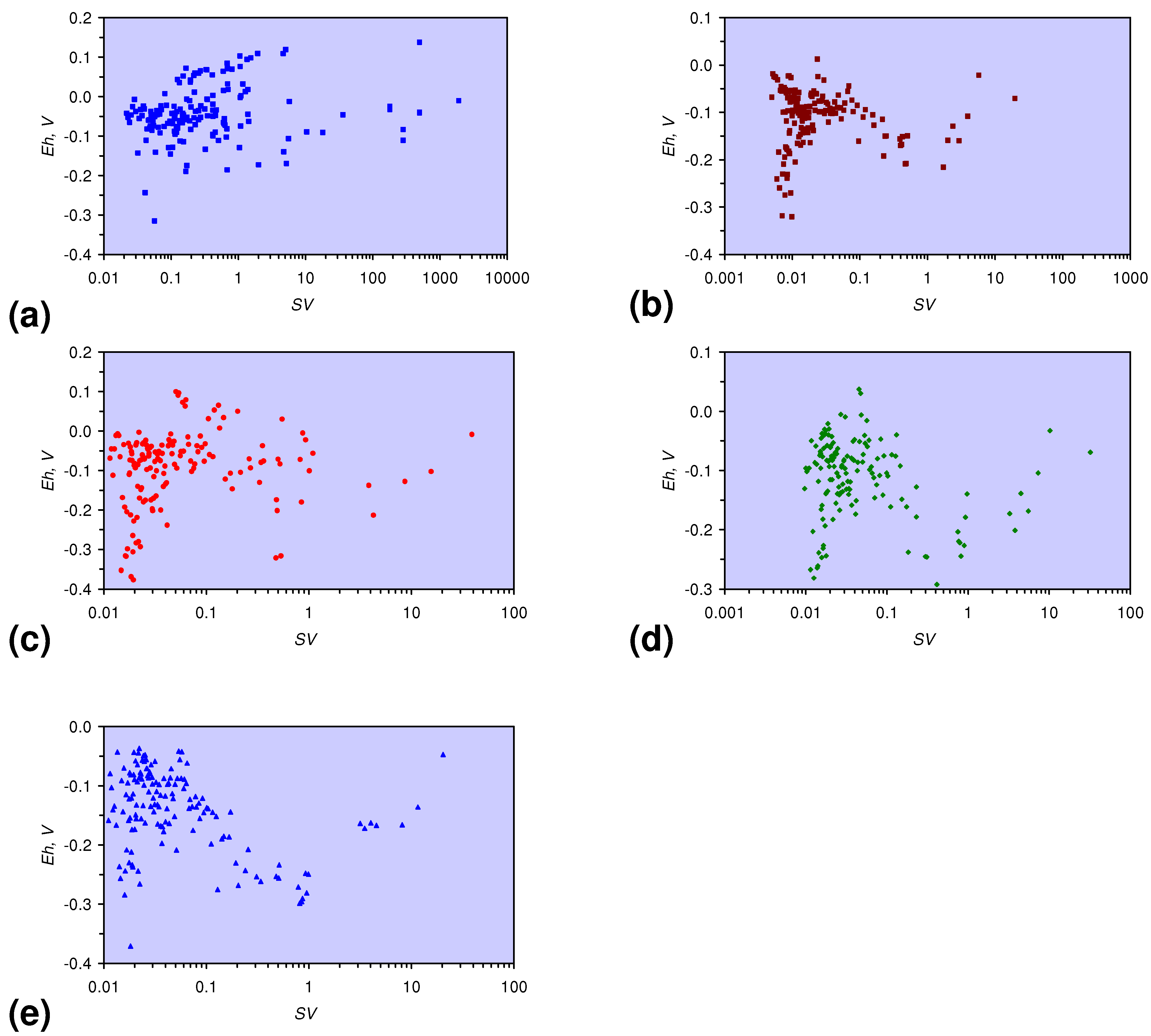
  • The EC:EC Initial ratio varies with both Eh and SV. The exact relationship varies with m-ZVM type (Figure 16).
  • The presence of more than 1 metal type (or a combination of n-ZVM and m-ZVM of the same metal type) reduces the variance associated with a specific parameter (e.g., Eh, pH, EC).
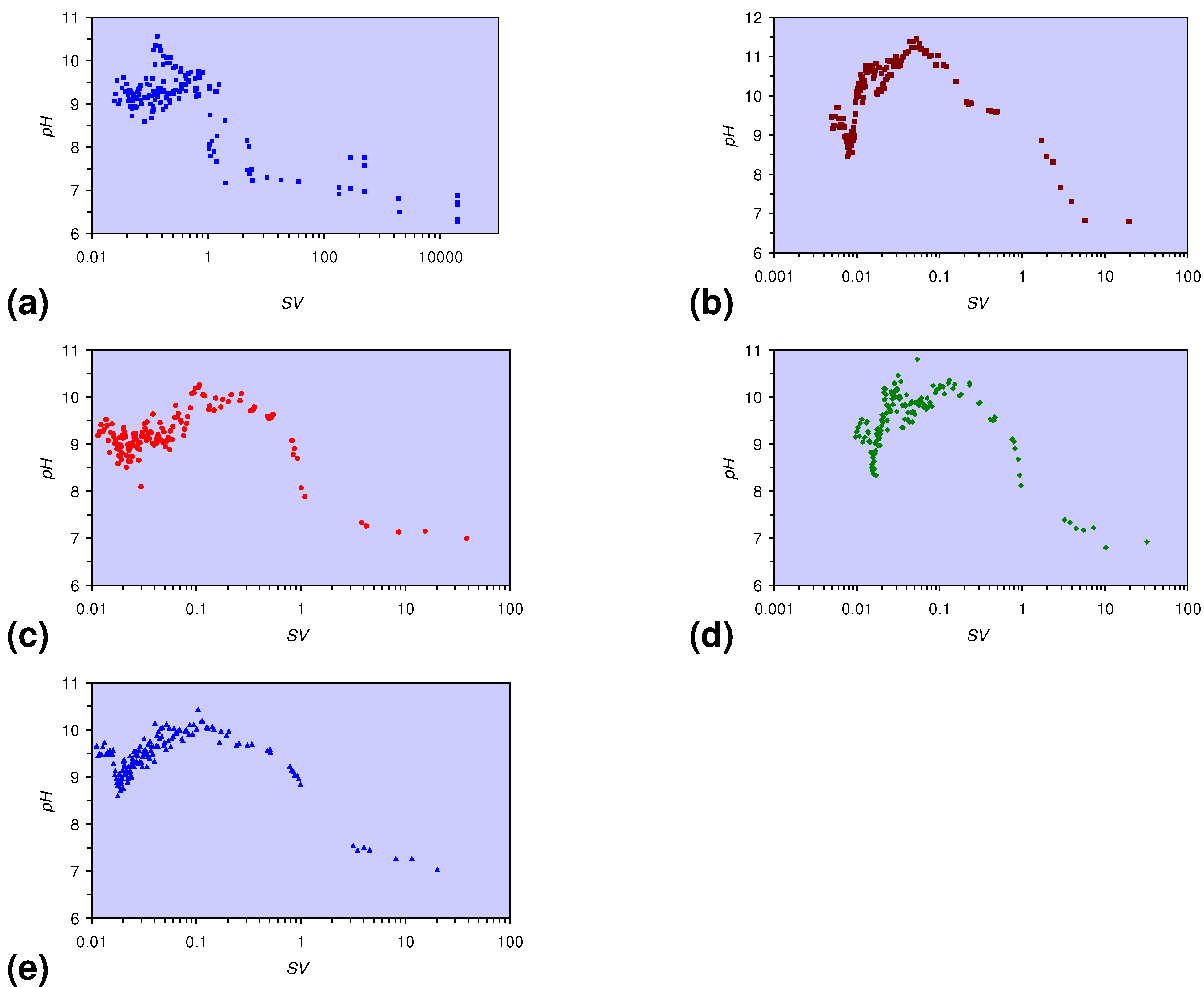
3.1.1. MWR1

Eh = 0.0113 × Log(SV) − 0.027: R2 = 0.201; EhInitial = 0.111 V
pH = −0.1189 × Log(SV > 6) + 7.7361; R2 = 0.511;
pH = −0.5243 × Log(0.13 < SV < 6) + 8.796; R2 = 0.508;
pH = 0.1887 × Log(SV < 0.13) + 9.743; R2 = 0.061; pHInitial = 6.43;
EC:ECInitial =0.0047 × Log(SV > 1) + 0.9457; R2 = 0.134;
EC:ECInitial = 0.0693 × Log(SV < 1) + 0.8791; R2 = 0.424; ECInitial = 0.339 mS cm−1;

3.1.2. MWR2

Eh = 0.036 × Log(SV > 1) − 0.1733; R2 = 0.732;
Eh = −0.0335 × Log(0.02 < SV < 1) − 0.1932; R2 = 0.629;
Eh = 0.0185 × Log(SV < 0.02) − 0.374; R2 = 0.005; EhInitial = 0.045 V
pH = −0.037 × Log(SV > 5) + 6.8954; R2 = 0.980;
pH = −0.8708 × Log(0.05 < SV < 5) + 8.787; R2 = 0.972;
pH = 0.5784 × Log(0.01 < SV < 0.05) + 12.89; R2 = 0.559;
pH = 4.9227 × Log(0.0077 < SV < 0.01) + 32.364; R2 = 0.725;
pH = −1.3165 × Log(SV < 0.0077) + 2.5779; R2 = 0.471; pHInitial = 6.65;
EC:ECInitial =−0.0096 × Log(SV > 1) + 1.0552; R2 = 0.647;
EC:ECInitial = 0.1153 × Log(0.1 < SV < 1) + 1.0281; R2 = 0.877;
EC:ECInitial = −0.1431 × Log(0.07 < SV < 0.1) + 0.487; R2 = 0.851;
EC:ECInitial = 0.2862 × Log(0.01 < SV < 0.07) + 1.6361; R2 = 0.948;
EC:ECInitial = −0.6428 × Log(0.0077 < SV < 0.01) – 2.5634; R2 = 0.734;
EC:ECInitial = 0.3692 × Log(SV < 0.0077) + 2.332: R2 = 0.961; ECInitial = 0.328 mS cm−1;

3.1.3. MWR3

Eh = 0.0432 × Log(SV > 1) −0.2198; R2 = 0.872;
Eh = −0.0359 × Log(0.08 < SV < 1) − 0.12; R2 = 0.145;
Eh = 0.0772 × Log(SV < 08) + 0.1764; R2 = 0.144; EhInitial = 0.078 V;
pH = −0.1724 × Log(SV > 1) + 7.7137; R2 = 0.781;
pH = −1.8857 × Log(0.5 < SV < 1) + 8.4663; R2 = 0.879;
pH = −0.2833 × Log(0.1 < SV < 0.5) + 9.4166; R2 = 0.590;
pH = 0.307 × Log(SV < 0.1) + 10.234: R2 = 0.263; pHInitial = 6.65;
EC:ECInitial = −0.0043 × Log(SV > 1) + 1.0532; R2 = 0.09;
EC:ECInitial = 0.2208 × Log(0.2 < SV < 1) + 1.0834; R2 = 0.896;
EC:ECInitial = 0.0468 × Log(0.025 < SV < 0.2) + 0.822; R2 = 0.354;
EC:ECInitial = 0.2477 × Log(SV < 0.025) + 1.563; R2 = 0.968; ECInitial = 0.331 mS cm−1;

3.1.4. MWR4

Eh = 0.0443 × Log(SV > 0.4) − 0.224; R2 = 0.787;
Eh = −0.0516 × Log(0.03 < SV < 0.4) − 0.2427; R2 = 0.297;
Eh = 0.052 × Log(SV < 0.03) + 0.097; R2 = 0.051; EhInitial = 0.043 V;
pH = −0.1624 × Log(SV > 1) +7.575; R2 = 0.620;
pH = −1.1926 × Log(0.2 < SV < 1) + 8.5343; R2 = 0.911;
pH = 0.2224 × Log(0.03 < SV < 0.2) + 10.569; R2 = 0.171;
pH = 2.4307 × Log(0.0155 < SV < 0.03) + 18.846; R2 = 0.744;
pH = −1.4766 × Log(SV < 0.0155) + 2.639; R2 = 0.450; pHInitial = 6.65;
EC:ECInitial = −0.0414 Log(SV > 1) + 1.2554; R2 = 0.765;
EC:ECInitial = 0.2253 × Log(0.02 < SV < 1) + 1.1981; R2 = 0.964;
EC:ECInitial = −0.4157 × Log(0.015 < SV < 0.02) – 1.209; R2 = 0.757;
EC:ECInitial = 0.4138 × Log(SV < 0.015) + 2.218; R2 = 0.846; ECInitial = 0.332 mS cm−1;

3.1.5. MWR5

Eh = 0.0597 × Log(SV > 0.8) − 0.2631; R2 = 0.967;
Eh = −0.0483 × Log(0.02 > SV < 0.8) − 0.2753; R2 = 0.459;
Eh = −0.0413 × Log(SV < 0.02) − 0.324: R2 = 0.009; EhInitial = 0.160 V;
pH = −0.1775 × Log(SV > 3) + 7.6906; R2 = 0.970;
pH = −0.6104 × Log(0.1 < SV < 3) + 8.8984; R2 = 0.900;
pH = 0.7137 × Log(0.0177 < SV < 0.1) + 11.897; R2 = 0.777;
pH = −1.6348 × Log(SV < 0.0177) + 2.4307: R2 = 0.583; pHInitial = 6.43;
EC:ECInitial =−0.0225 × Log(SV > 1) + 1.1652; R2 = 0.761;
EC:ECInitial = 0.2253 × Log(0.04 < SV < 1) + 1.1281; R2 = 0.979;
EC:ECInitial = 0.0174 × Log(0.02 < SV < 0.04) + 0.5314; R2 = 0.020;
EC:ECInitial = 0.3838 × Log(SV < 0.02) + 1.9909; R2 = 0.930;
ECInitial = 0.334 mS cm−1; EC:ECInitial = Observed EC/ECInitial.
Figure 11. pH vs. SV. (a) MWR1; n = 172, t = 136,773 min; (b) MWR2; n = 157, t = 138,134 min; (c) MWR3; n = 157, t = 135319 min; (d) MWR4; n = 155, t = 136,701 min; (e) MWR5; n = 152, t = 135,405 min; t = test duration, n = number of measurements. SV = effective diffusion space velocity (m3 H2O h−1 t−1 m-ZVM).
Sustainability 02 02988 g011
Figure 12. Eh vs. SV. (a) MWR1; (b) MWR2; (c) MWR3; (d) MWR4; (e) MWR5.
Sustainability 02 02988 g012
Figure 13. EC:EC Initial vs. SV. (a) MWR1; (b) MWR2; (c) MWR3; (d) MWR4; (e) MWR5.
Sustainability 02 02988 g013
Figure 14. Eh vs. pH. (a) MWR1; (b) MWR2; (c) MWR3; (d) MWR4; (e) MWR5; Arrow indicates direction of decreasing SV. Redox boundaries from [73].
Sustainability 02 02988 g014
Figure 15. EC:ECInitial vs. pH. (a) MWR1; (b) MWR2; (c) MWR3; (d) MWR4; (e) MWR5; Arrows indicate direction of decreasing SV.
Sustainability 02 02988 g015
Figure 16. EC:ECInitial vs. Eh. (a) MWR1; (b) MWR2; (c) MWR3; (d) MWR4; (e) MWR5; Arrows indicate direction of decreasing SV.
Sustainability 02 02988 g016

3.2. Continuous Flow Reactor Results: n-ZVM

The product water composition is described by a series of regression relationships. They allow prediction of the product water Eh and pH as a function of SV. They demonstrate a general trend of pH increasing with decreasing SV (Figure 17) and Eh remaining stable or increasing with decreasing SV (Figure 18). The ratio EC:ECFeed shows a reduction with decreasing SV (Figure 19).
The n-Fe0 (DR1) creates (Figure 20a) redox environments around the NH4+: NOx redox fence [72] at high SV and in the Fe2O3 stability zone [72] at low SV. The addition of n-Cu0 (DR2) or n-Cu0 + n-Al0 (DR3) focuses the redox environment of the product water into the Fe2O3 stability zone (Figure 20b, c). SV decreases as permeability decreases (Figure 3). From Figure 20a it is apparent that if a high permeability can be maintained through the ZVM bed (e.g., Figure 4), then it will be possible to maintain the product water composition around the NH4+: NOx redox fence [73].
The n-ZVM combination controls whether the EC:ECFeed ratio decreases or increases with increasing pH (Figure 21). However, the EC:ECFeed ratio decreases with increasing Eh (Figure 22). Throughout the continuous flow tests the n-ZVM increased the product water pH relative to the feed water pH (Figure 23) and decreased the product water Eh relative to the feed Eh (Figure 24).

3.2.1. DR1

Eh = −0.032 × Log(SV) − 0.0165; R2 = 0.45;
pH = −0.3503 × Log(SV) + 8.132; R2 = 0.41;
EC:ECFeed = 0.0788 × Log(SV) + 0.9953; R2 = 0.7;

3.2.2. DR2

Eh = −0.019 × Log(SV) + 0.0439; R2 = 0.13;
pH = −0.2035 × Log(SV) + 7.6222; R2 = 0.10;
EC:ECFeed = 0.0158 × Log(SV) + 1.0243; R2 = 0.065;

3.2.3. DR3

Eh = 0.0077 × Log(SV) + 0.0253; R2 = 0.17;
pH = −0.6108 × Log(SV) + 8.1608; R2 = 0.52;
EC:ECFeed = −0.0284 × Log(SV) + 0.7803; R2 = 0.03;
The Feed Composition was Eh (mean = 0.134 V; SD = 0.047 V); pH (mean = 6.42; SD = 0.193); EC (mean = 0.273 mS cm−1; SD = 0.018 mS cm−1).
Figure 17. SV vs. pH: n-ZVM. (a) DR1 (n = 117; test duration = 112,473 min); (b) DR2 (n = 117; test duration = 112,473 min); (c) DR3 (n = 112; test duration = 109,916 min).
Sustainability 02 02988 g017
Figure 18. SV vs. Eh (V): n-ZVM. (a) DR1; (b) DR2; (c) DR3.
Sustainability 02 02988 g018
Figure 19. SV vs. EC:ECFeed Ratio: n-ZVM. (a) DR1; (b) DR2; (c) DR3.
Sustainability 02 02988 g019
Figure 20. Eh vs. pH: n-ZVM. (a) DR1; (b) DR2; (c) DR3: Feed water = blue triangles. Redox boundaries from [73].
Sustainability 02 02988 g020
Figure 21. EC:ECFeed vs. pH: n-ZVM. (a) DR1; (b) DR2; (c) DR3.
Sustainability 02 02988 g021
Figure 22. EC:ECFeed vs. Eh: n-ZVM. (a) DR1; (b) DR2; (c) DR3.
Sustainability 02 02988 g022
Figure 23. SV vs. [pHProduct – pHFeed]: n-ZVM. (a) DR1; (b) DR2; (c) DR3.
Sustainability 02 02988 g023
Figure 24. SV vs. [EhProduct – EhFeed]: n-ZVM. (a) DR1; (b) DR2; (c) DR3.
Sustainability 02 02988 g024

3.3. Continuous Flow Reactor Results: m-ZVM

The observed regression relationships with SV allow prediction of the Eh and pH of the treated water. Specific observations are:
  • pH increases with decreasing SV (Figure 25). The presence of m-Cu0, or m-Cu0 + m-Al0, decreases the increase in pH with decreasing SV, and reduces the variability associated with pH at a specific SV (Figure 25).
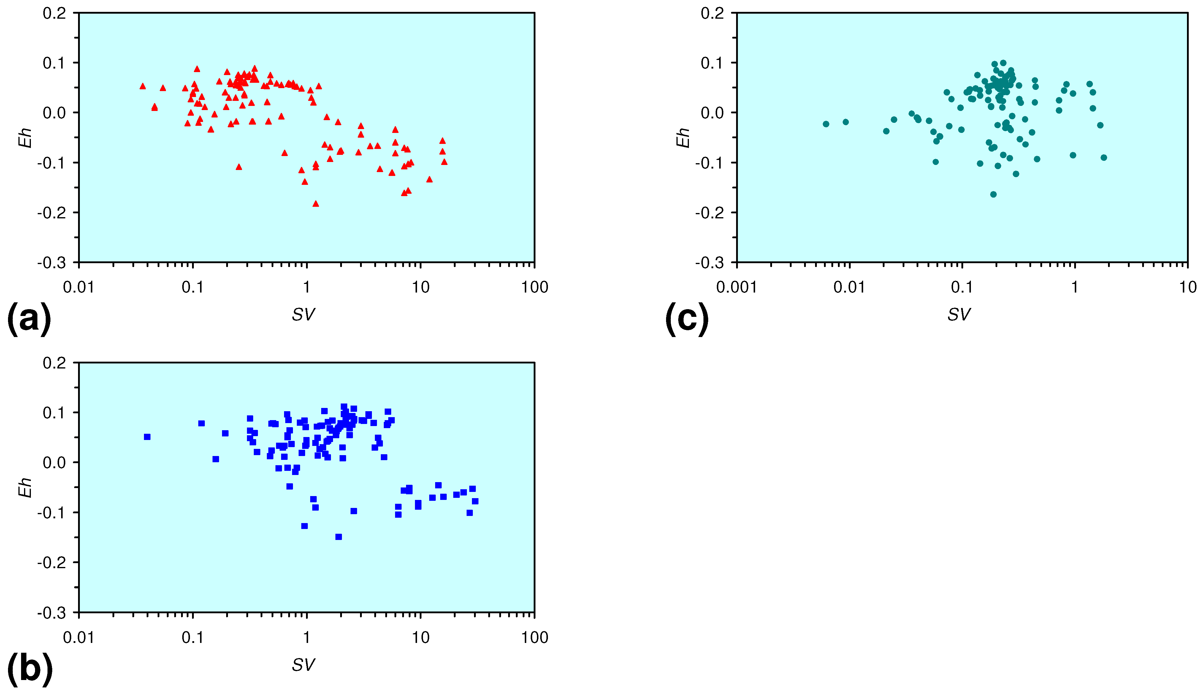
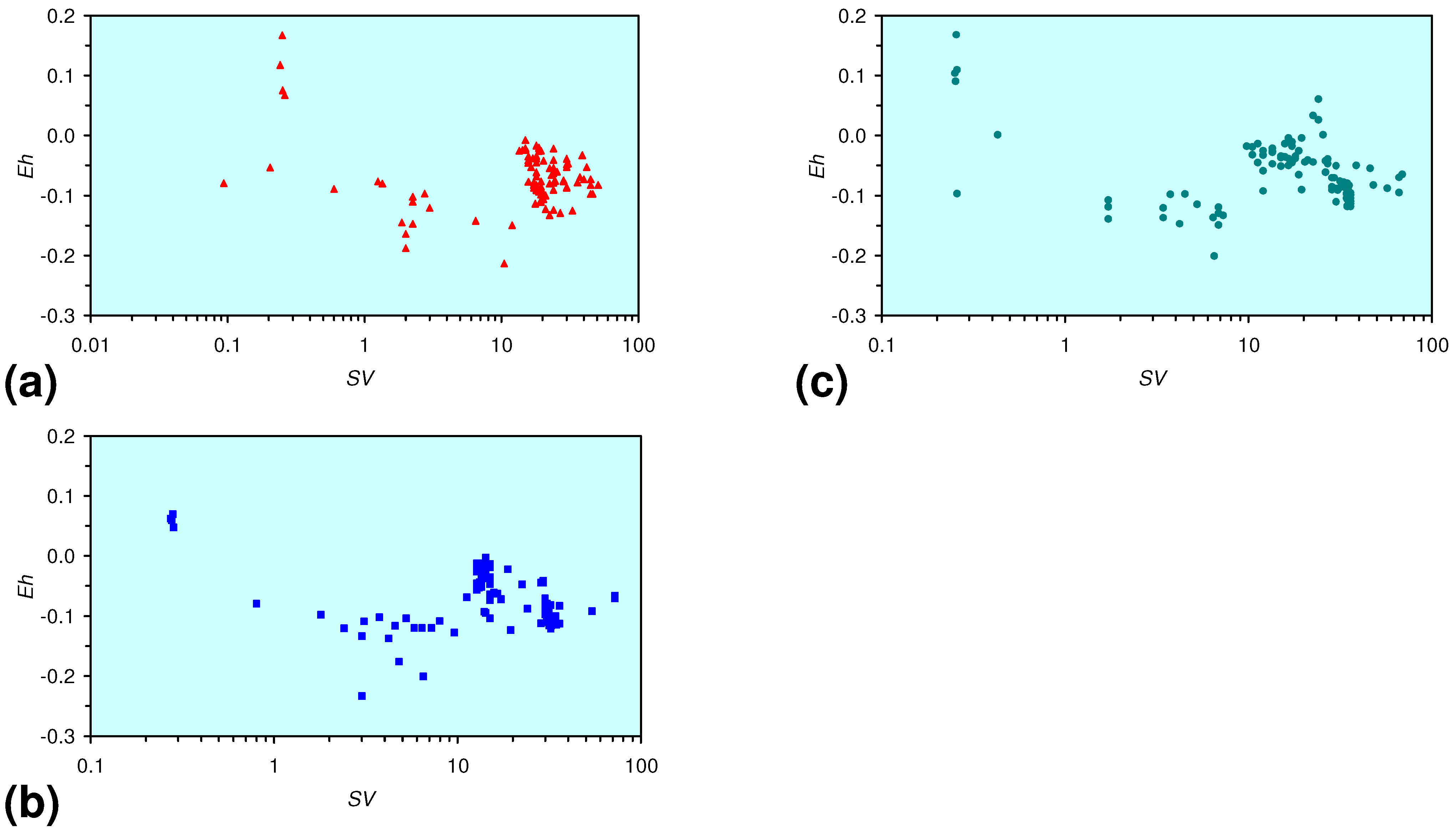
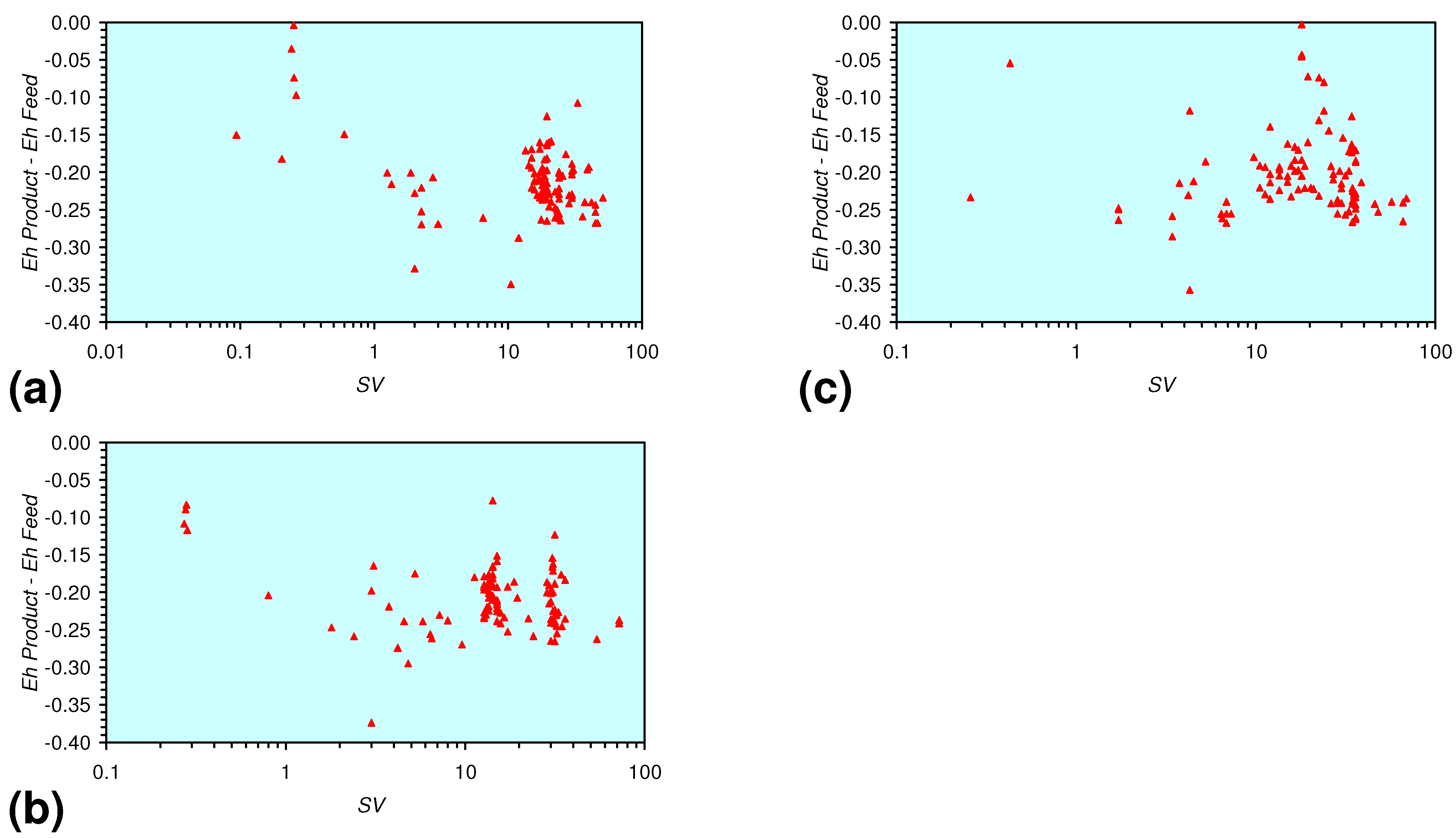
  • There is a general trend of increasing Eh with decreasing SV. The lowest Eh values were observed over the range 1 < SV < 10 (Figure 26).
  • The EC of the product water was about 10%–20% higher than the EC of the feed water for m-Fe0 (Figure 27). The addition of m-Cu0, or m-Cu0 + m-Al0 decreased the increase in product water EC (Figure 27). The increase in EC is due to the presence of Fe ions in the product water.
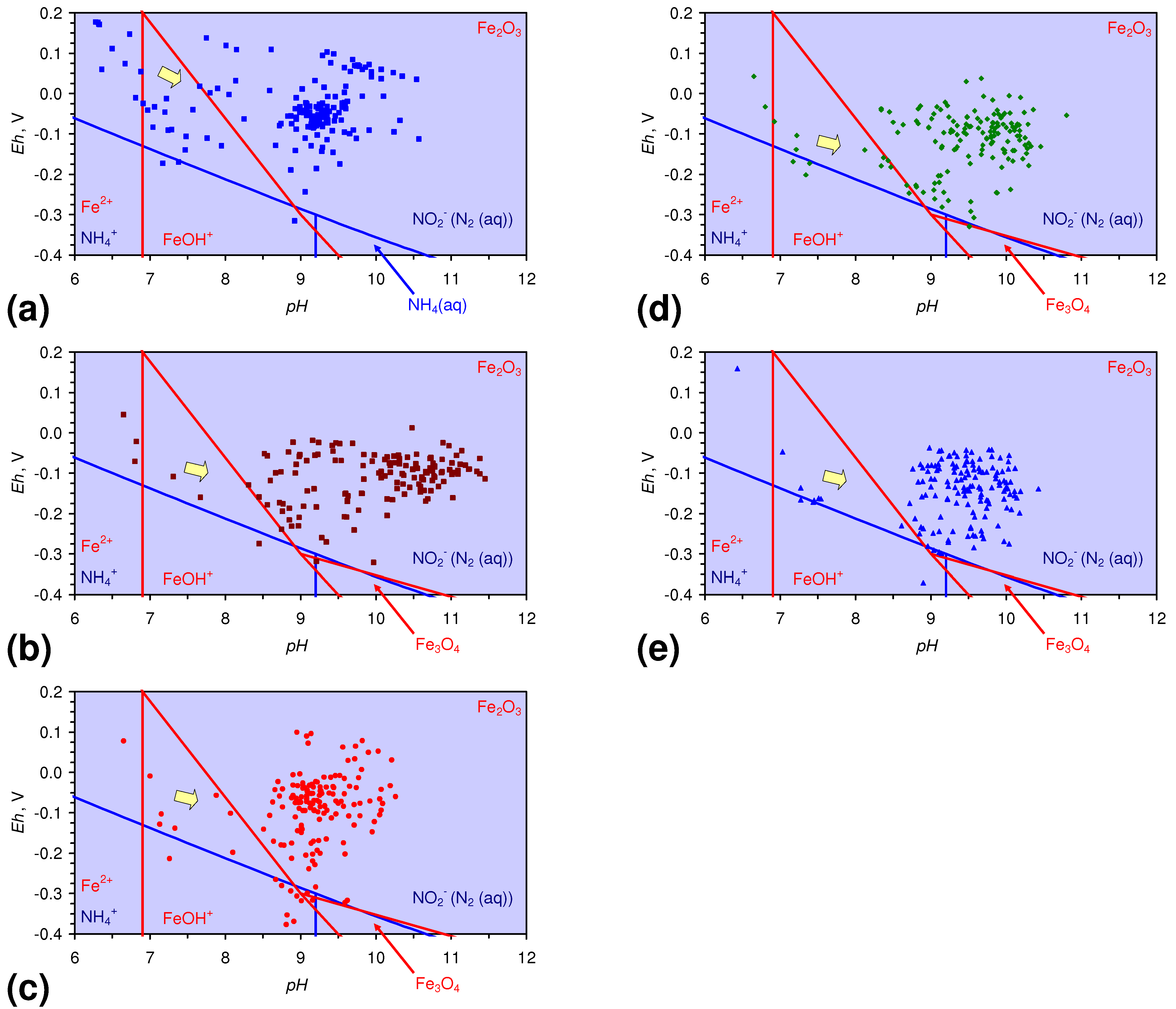
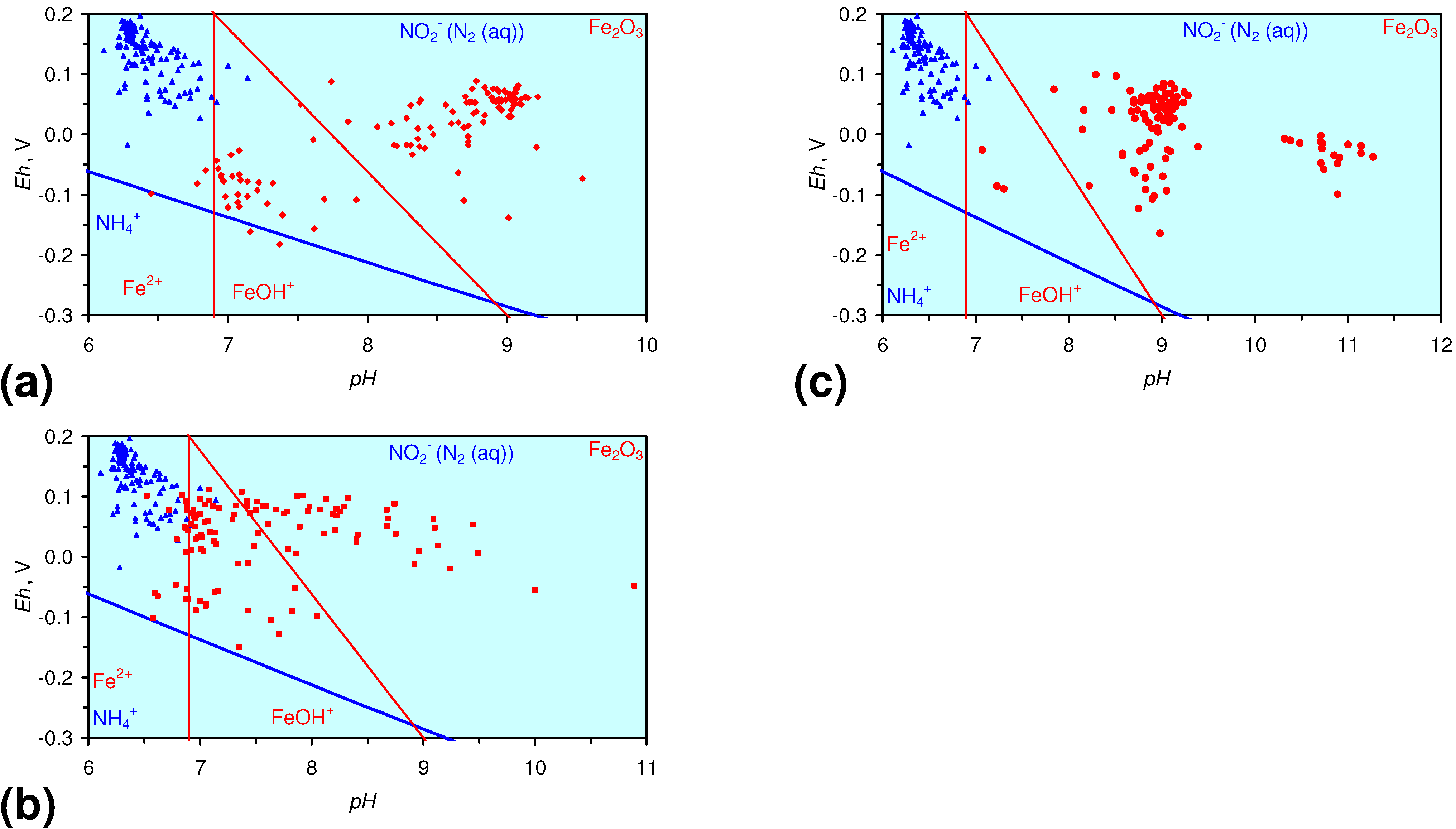
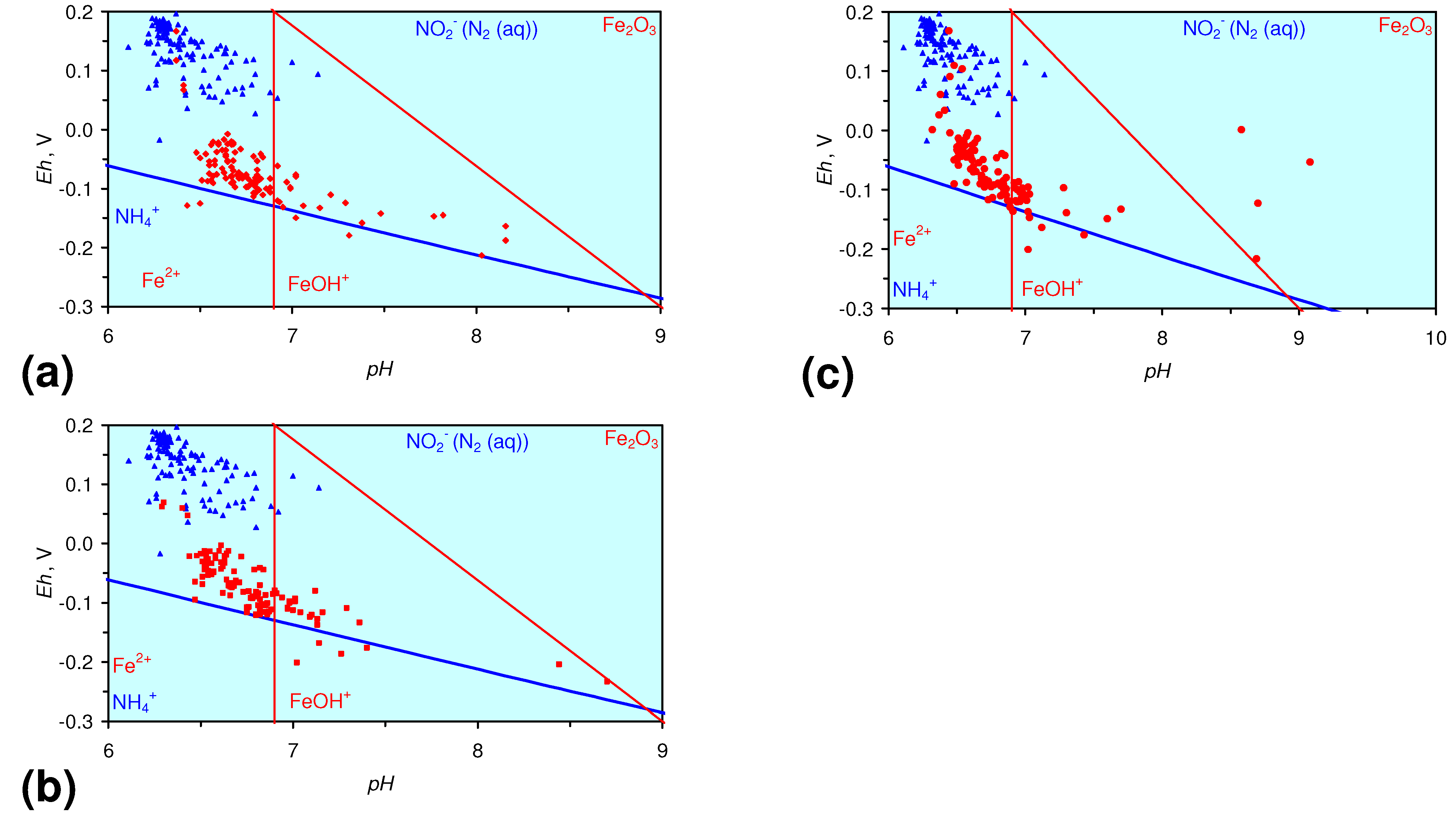
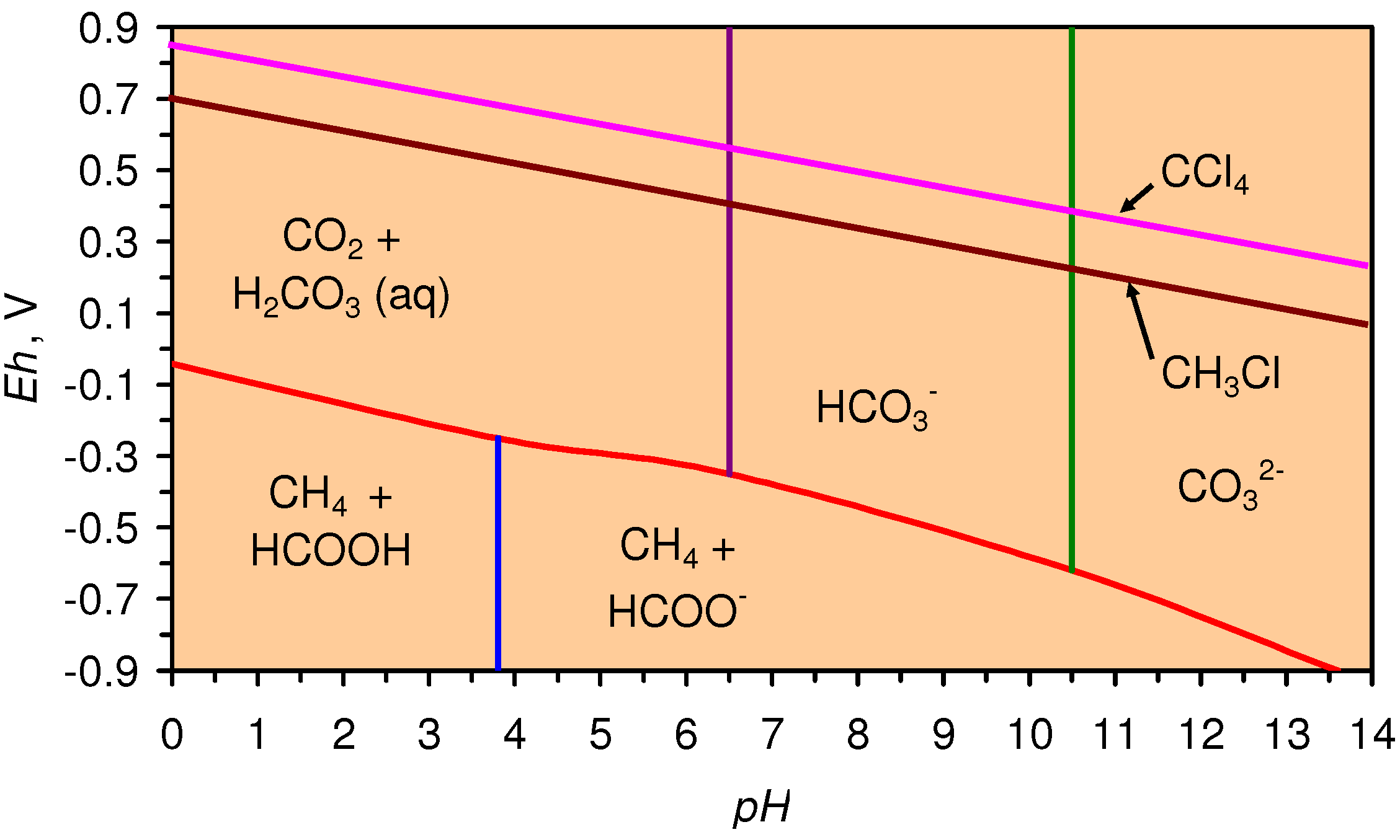
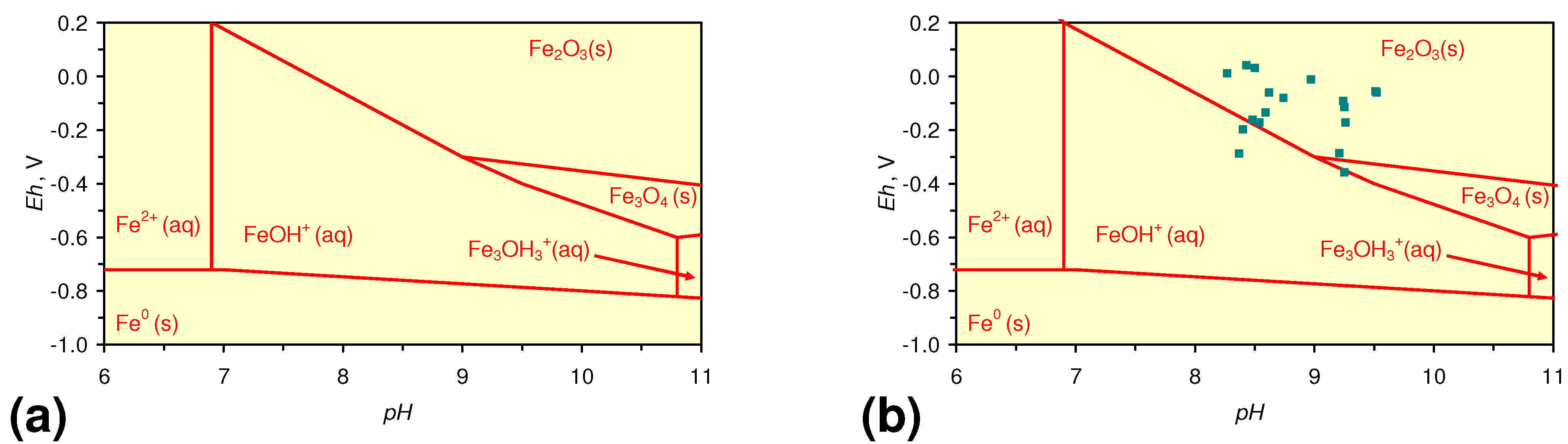
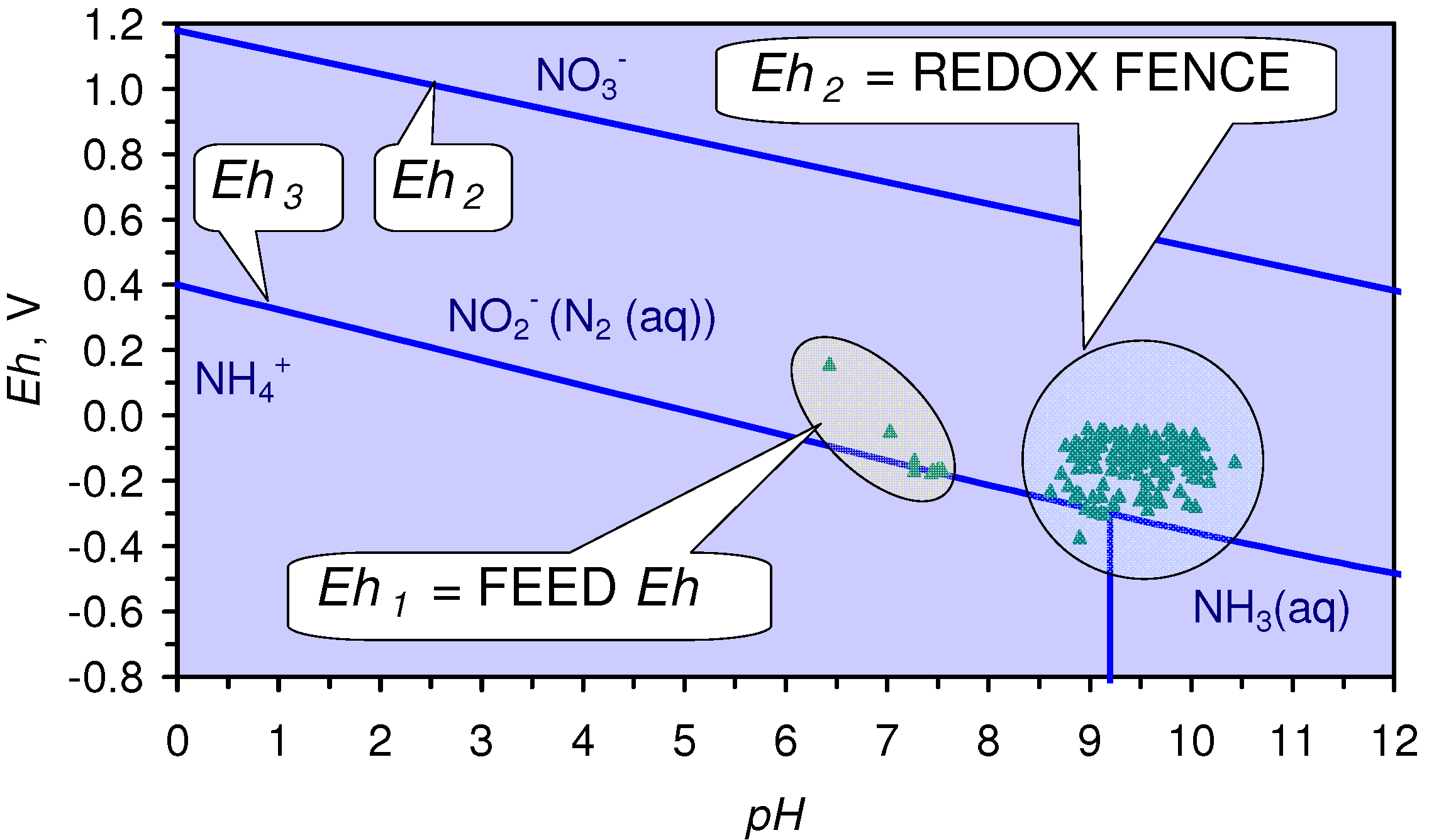
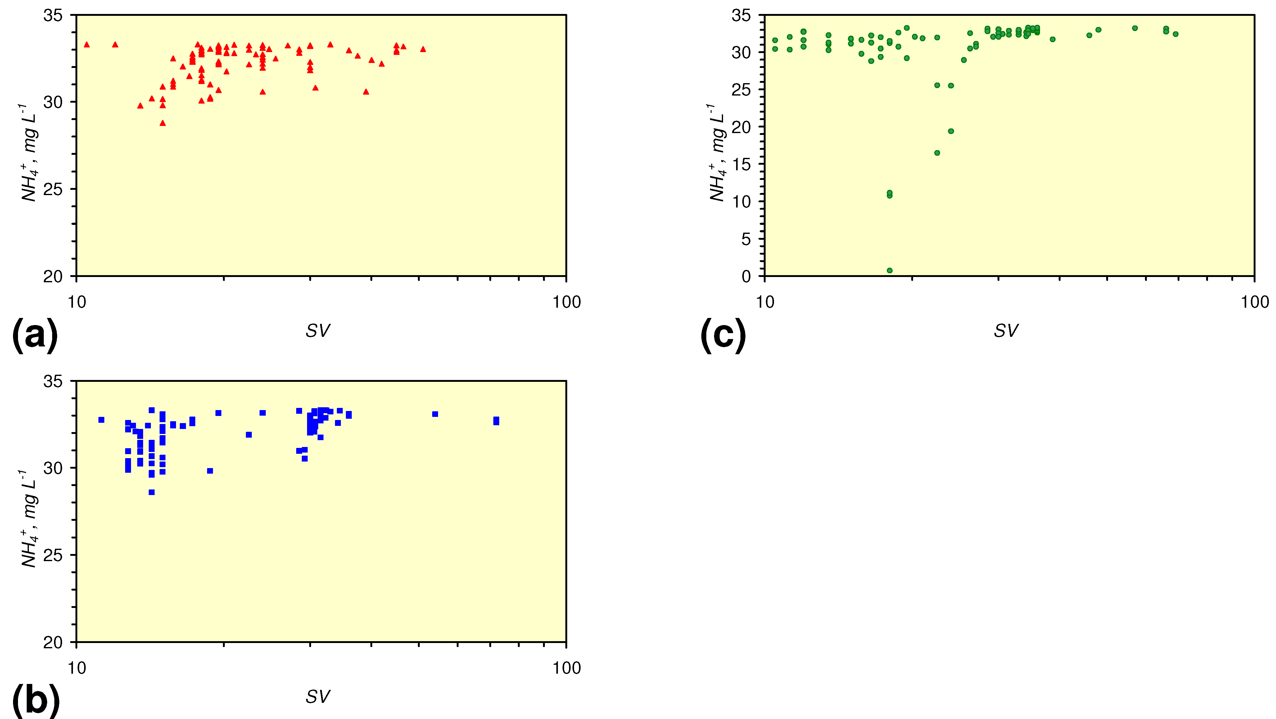
  • The m-ZVM consistently moves the product water Eh:pH to the NH4+:NOx redox fence (Figure 28).
  • BR2 and BR3 (Figure 29) show a consistent trend of increasing EC (Fe ions) with increasing pH.
  • The release of Fe ions (increase in EC) reaches a maximum level when the Eh is between −0.1 and −0.15 V (Figure 30). The addition of m-Cu0, or m-Cu0 + m-Al0 decreased the variability associated with Fe ion formation (Figure 30).
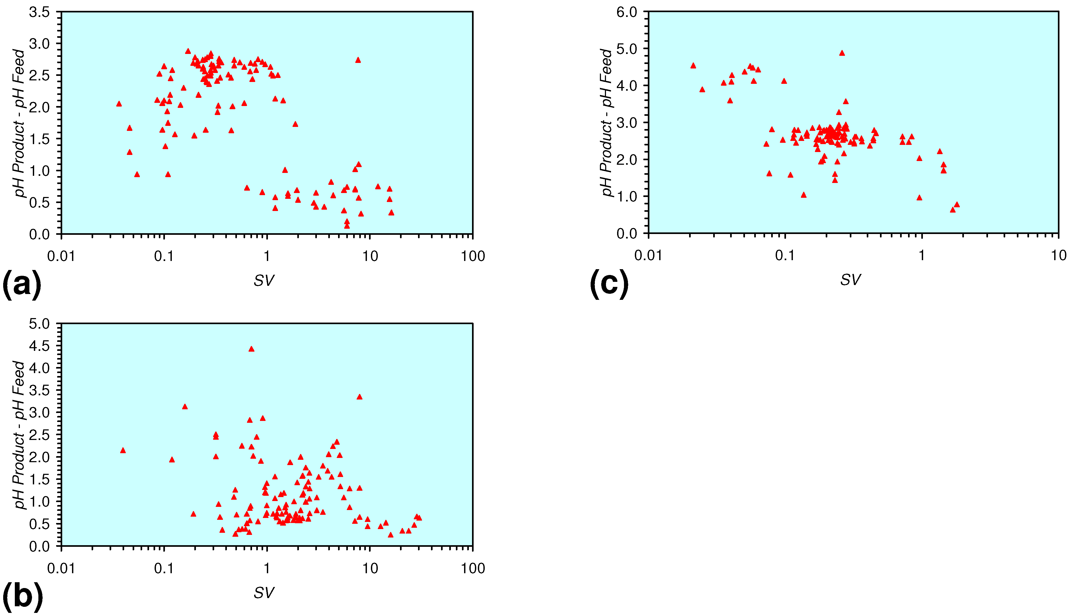
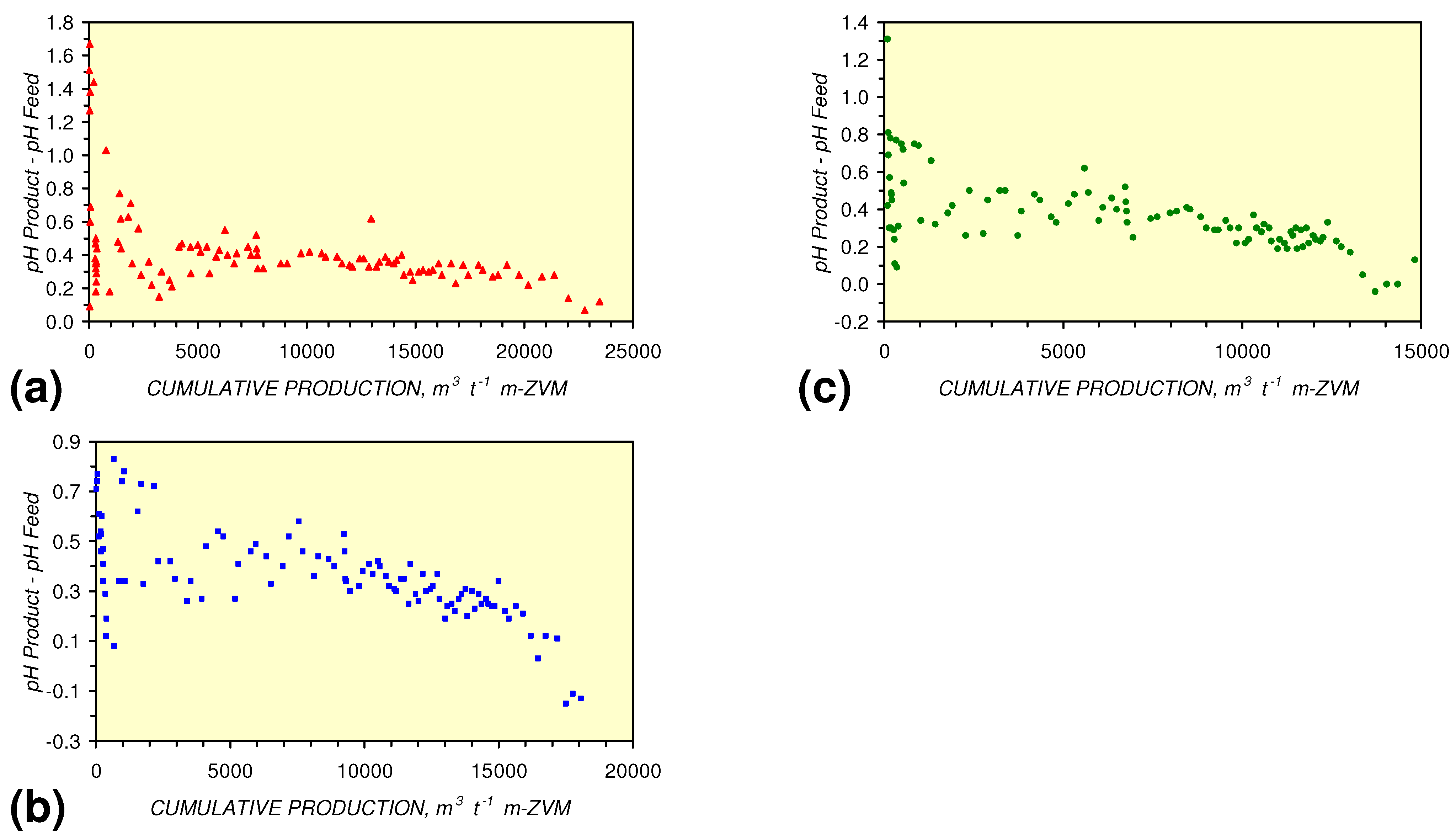
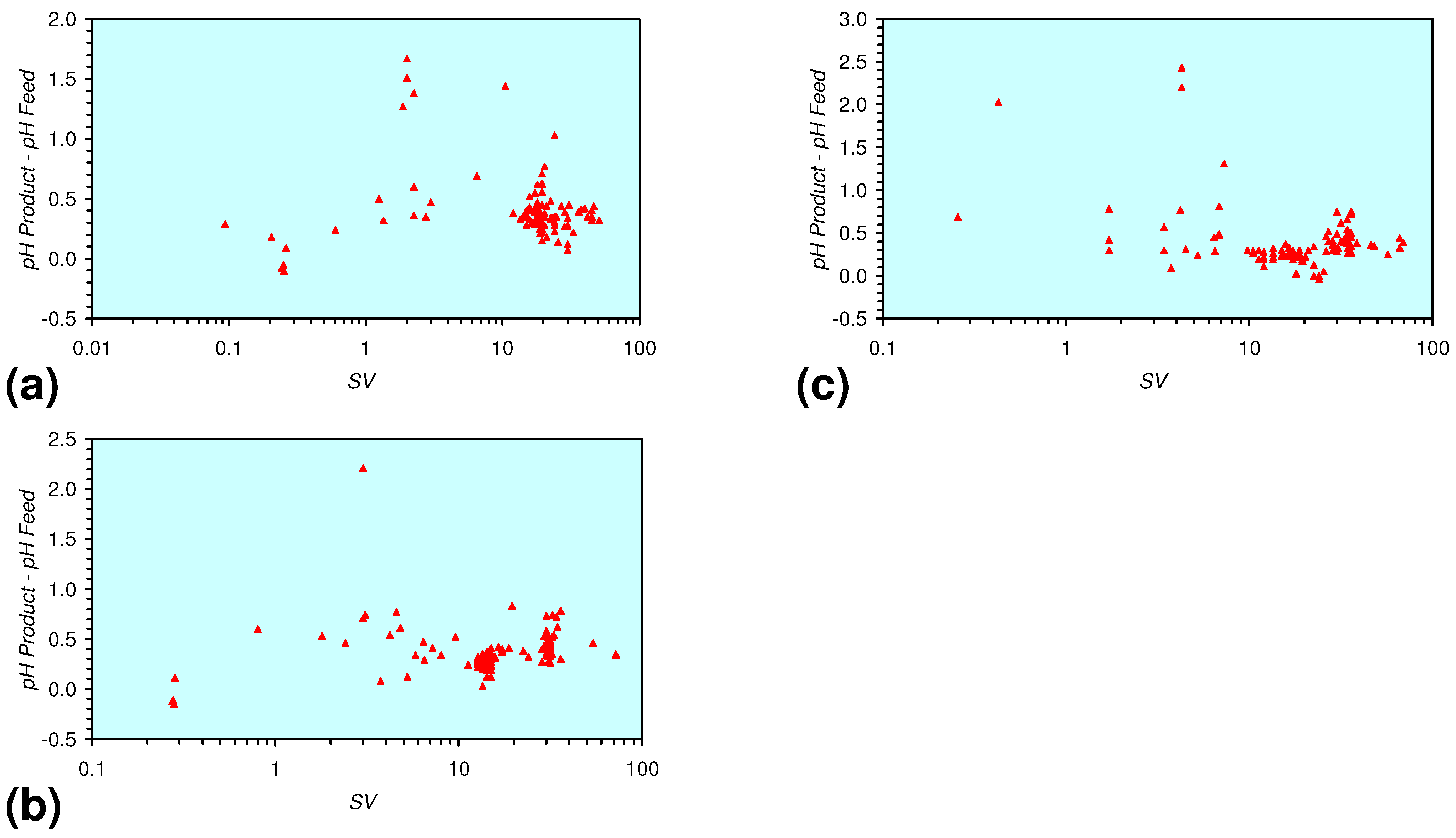
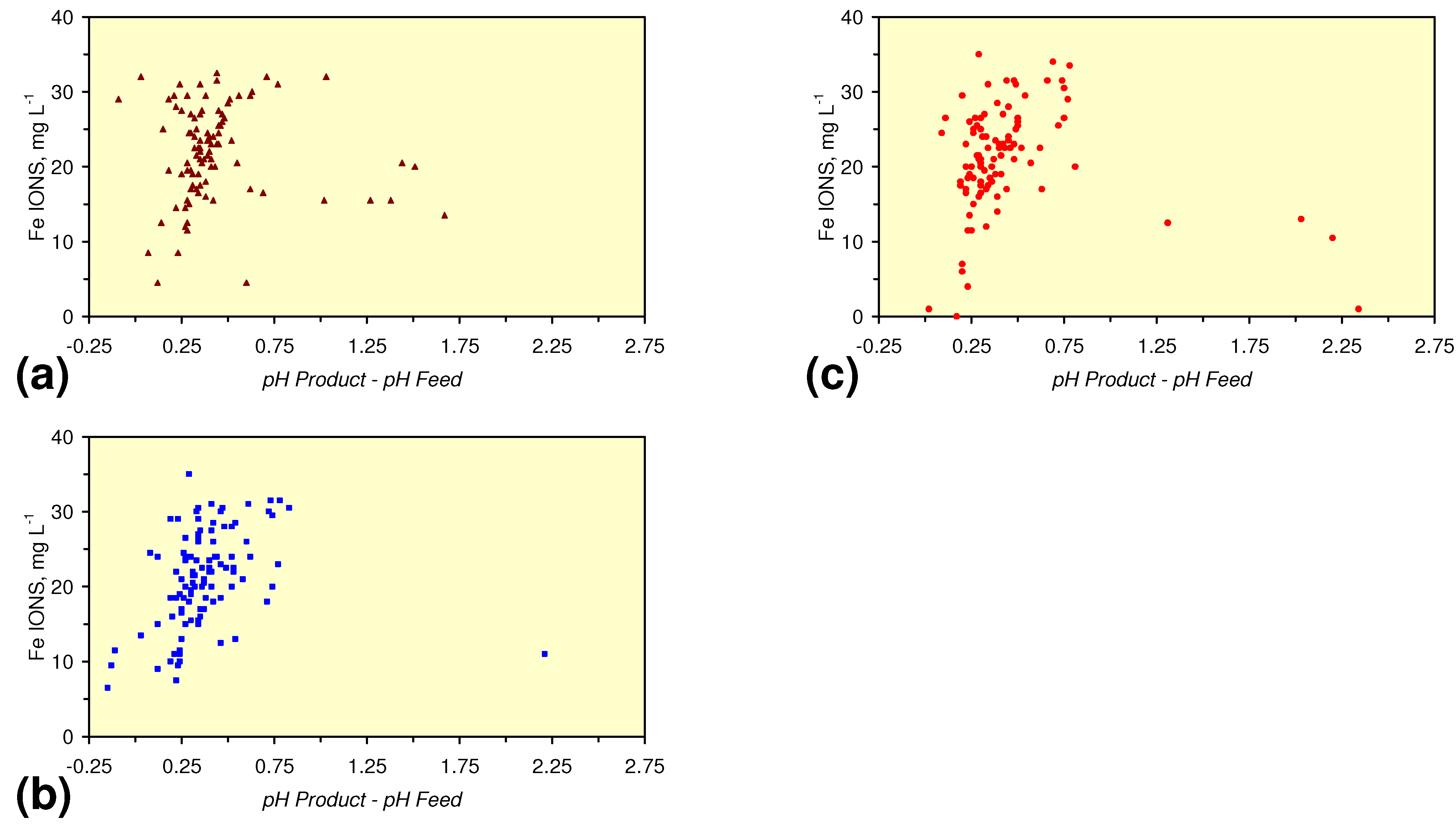
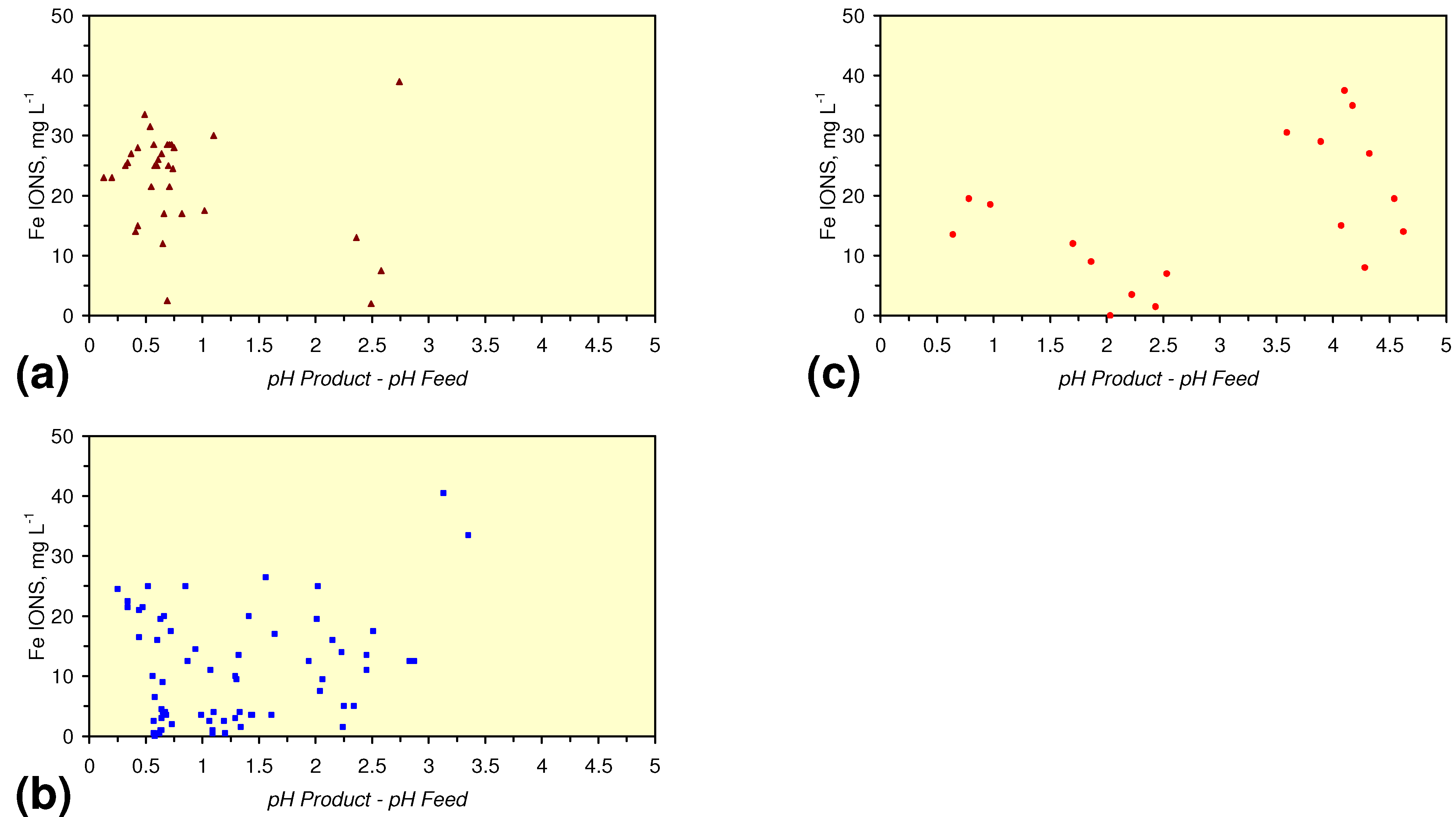
  • m-Fe0, or m-Fe0 + m-Cu0 show a general trend where [pHproductpHFeed] increases with decreasing SV to a maximum value where 1 < SV < 10 (Figure 31). [pHproductpHFeed] then decreases with decreasing SV. The addition of m-Al0 resulted in [pHproductpHFeed] increasing with decreasing SV when SV < 1 (Figure 31).
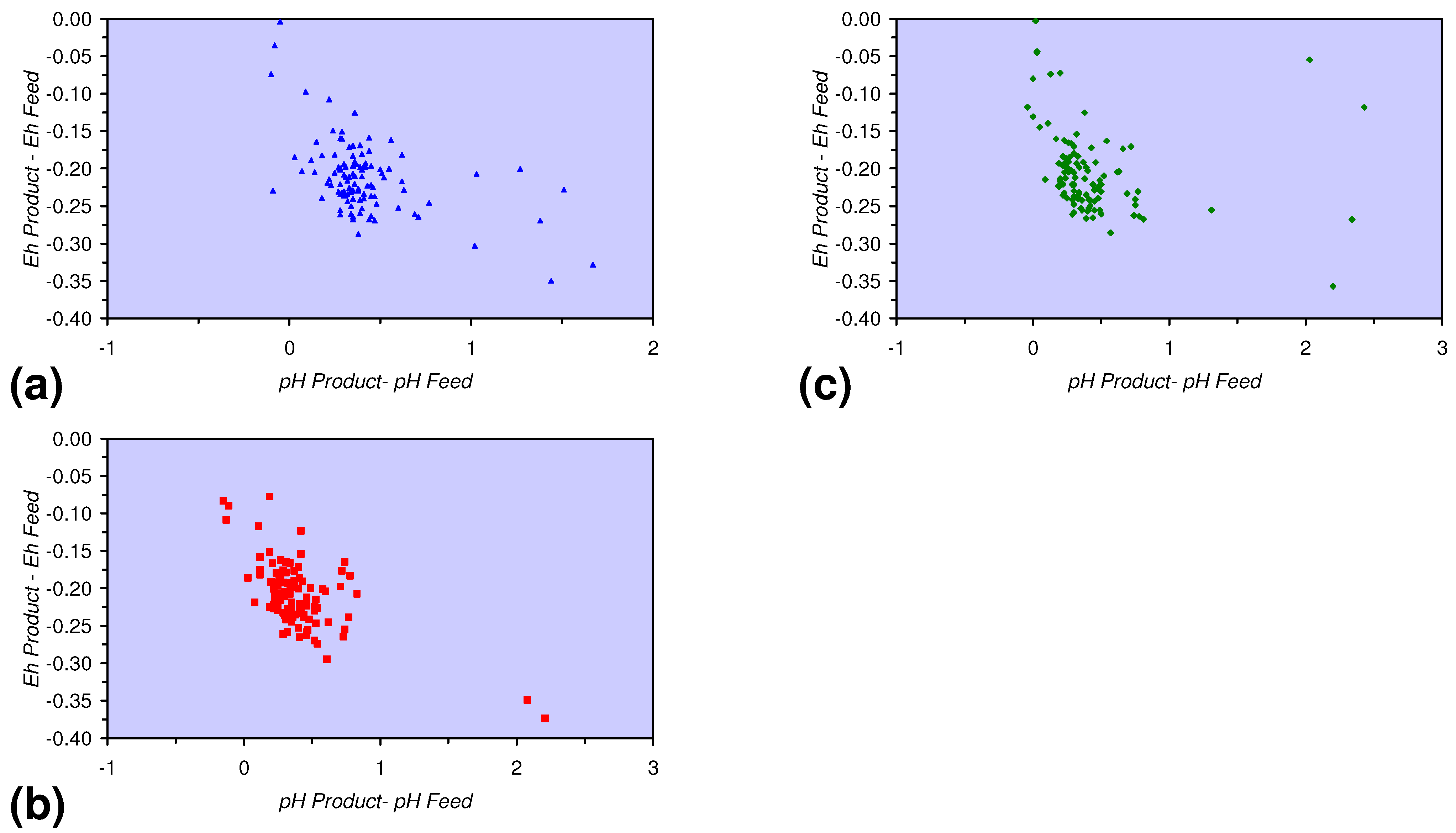
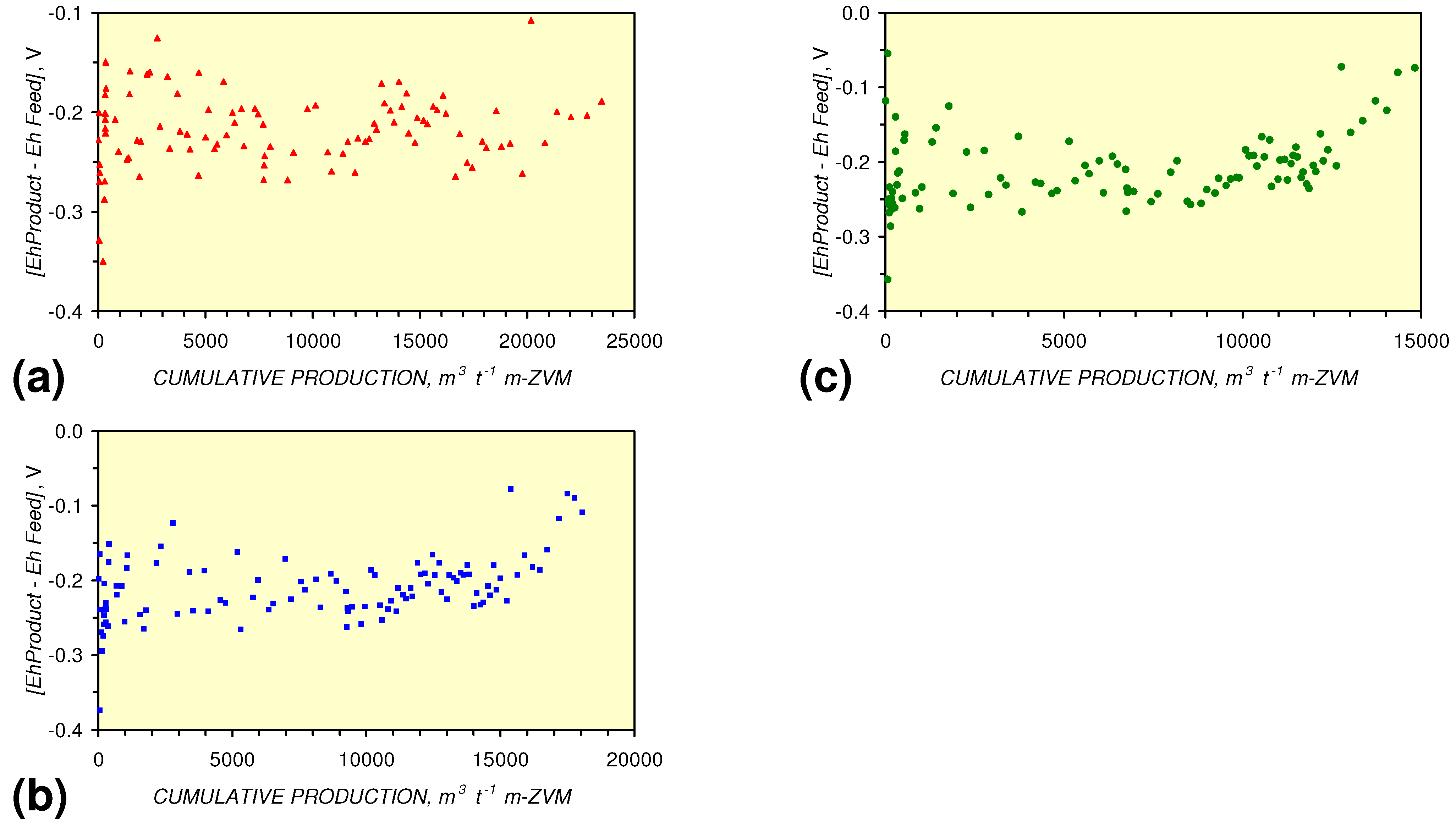
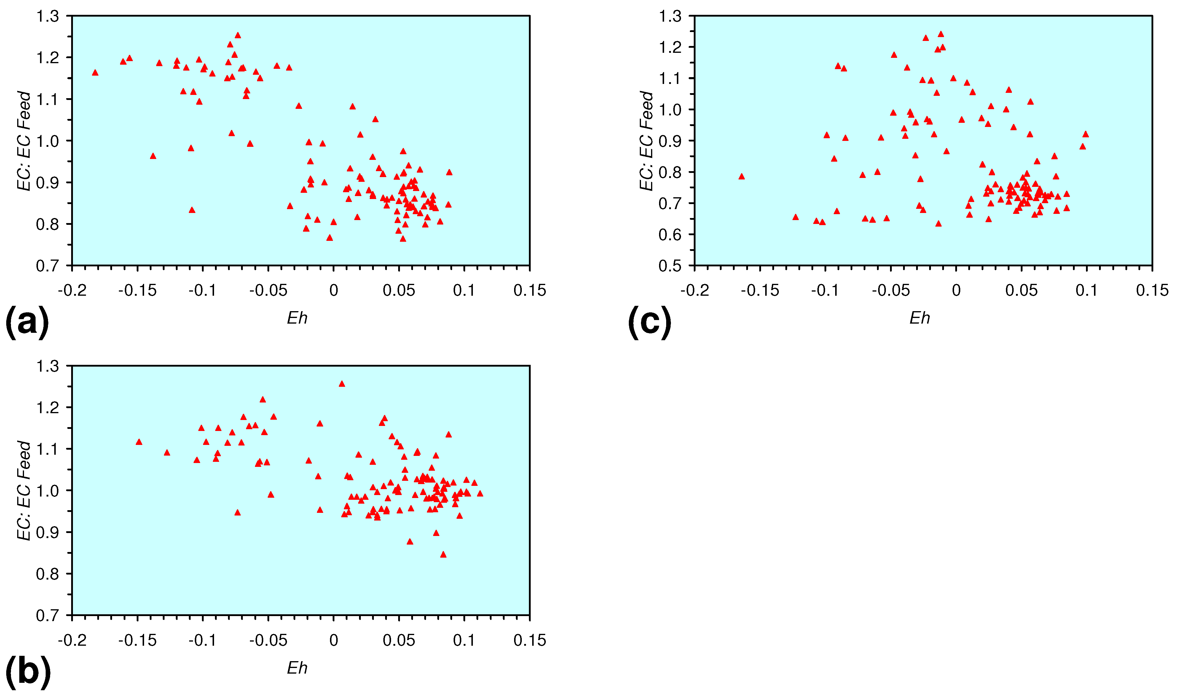
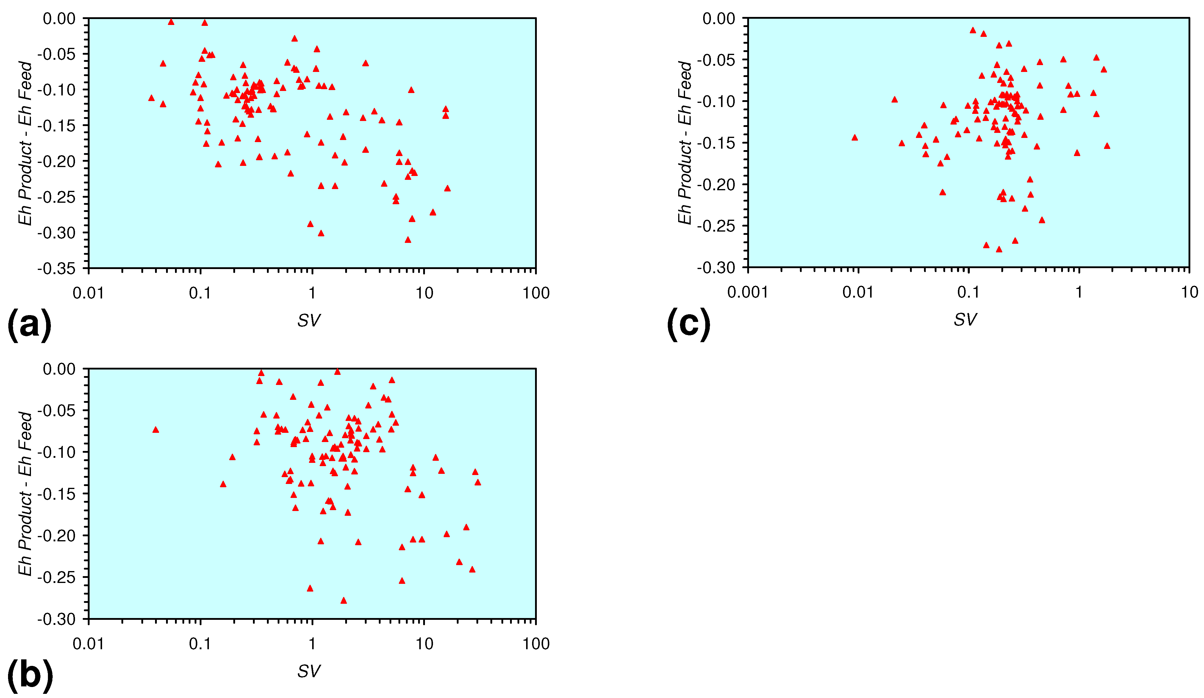
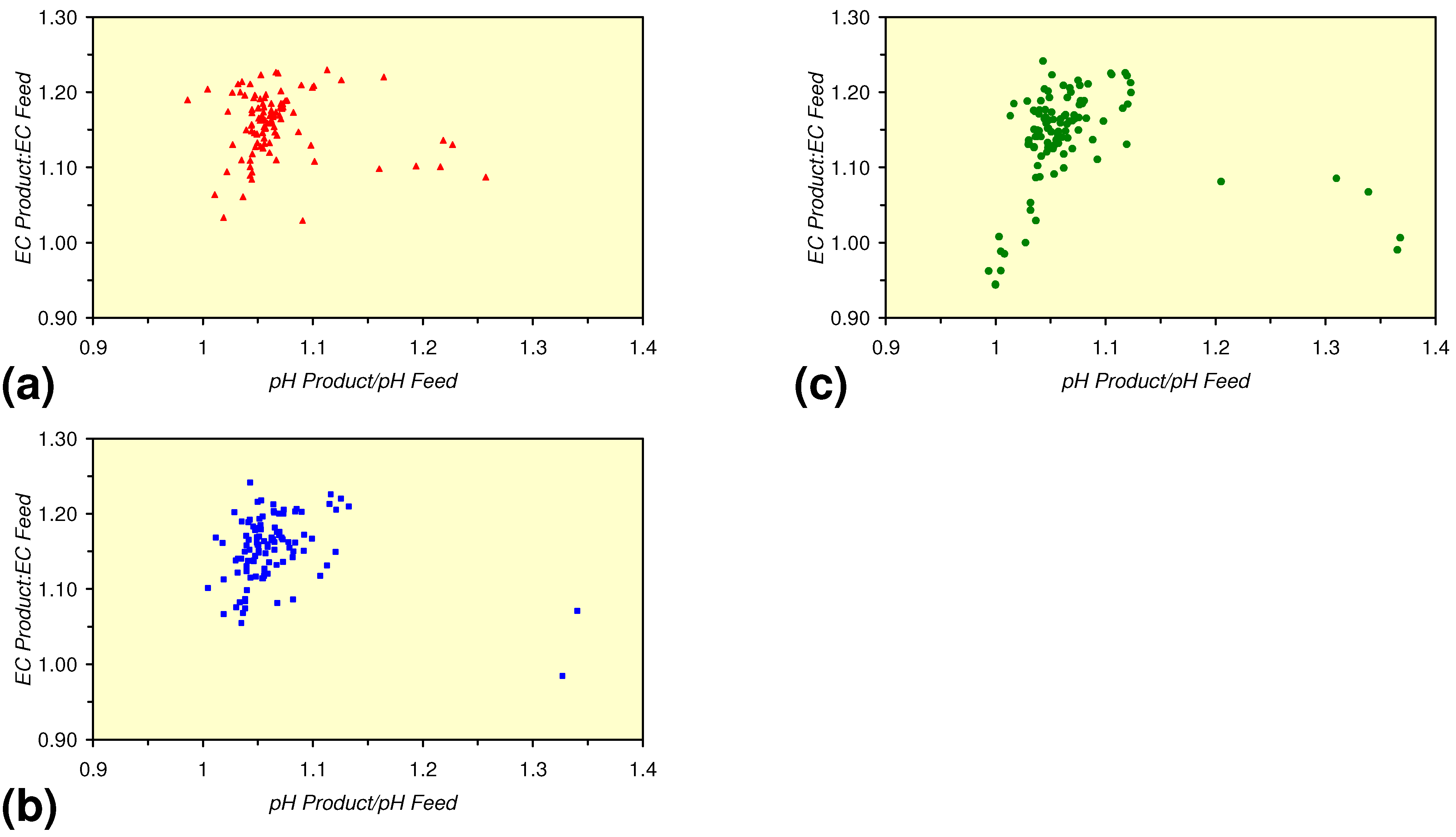
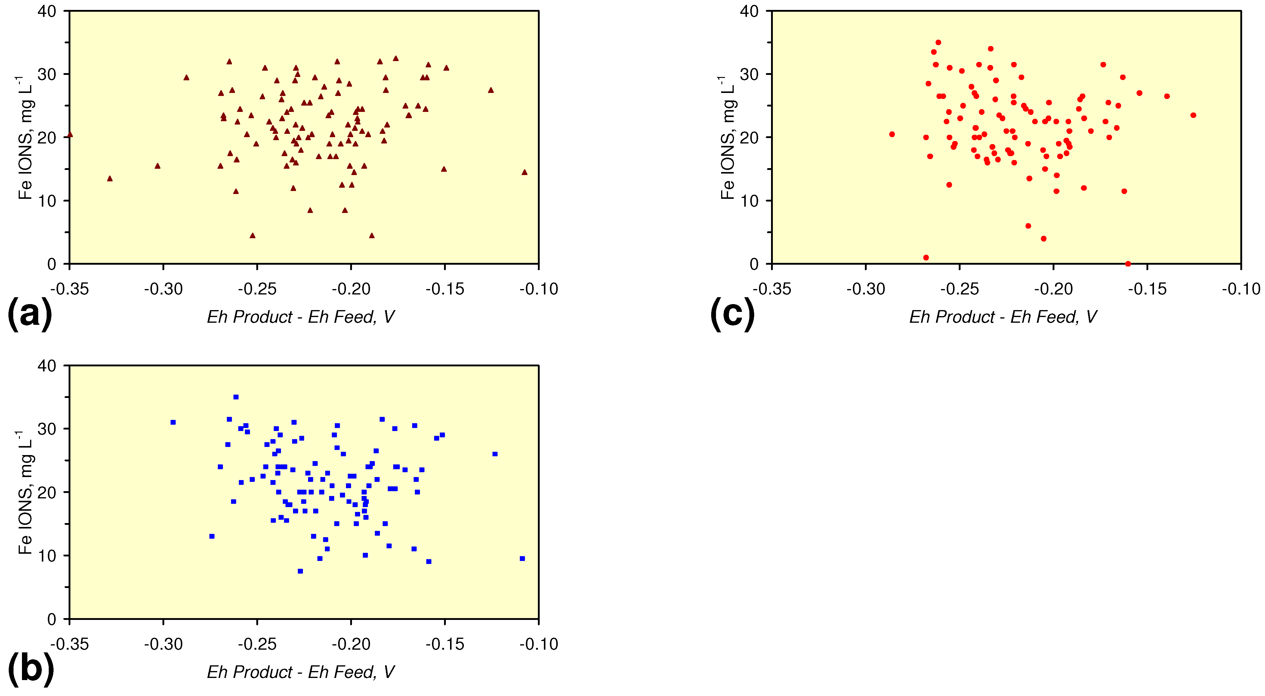
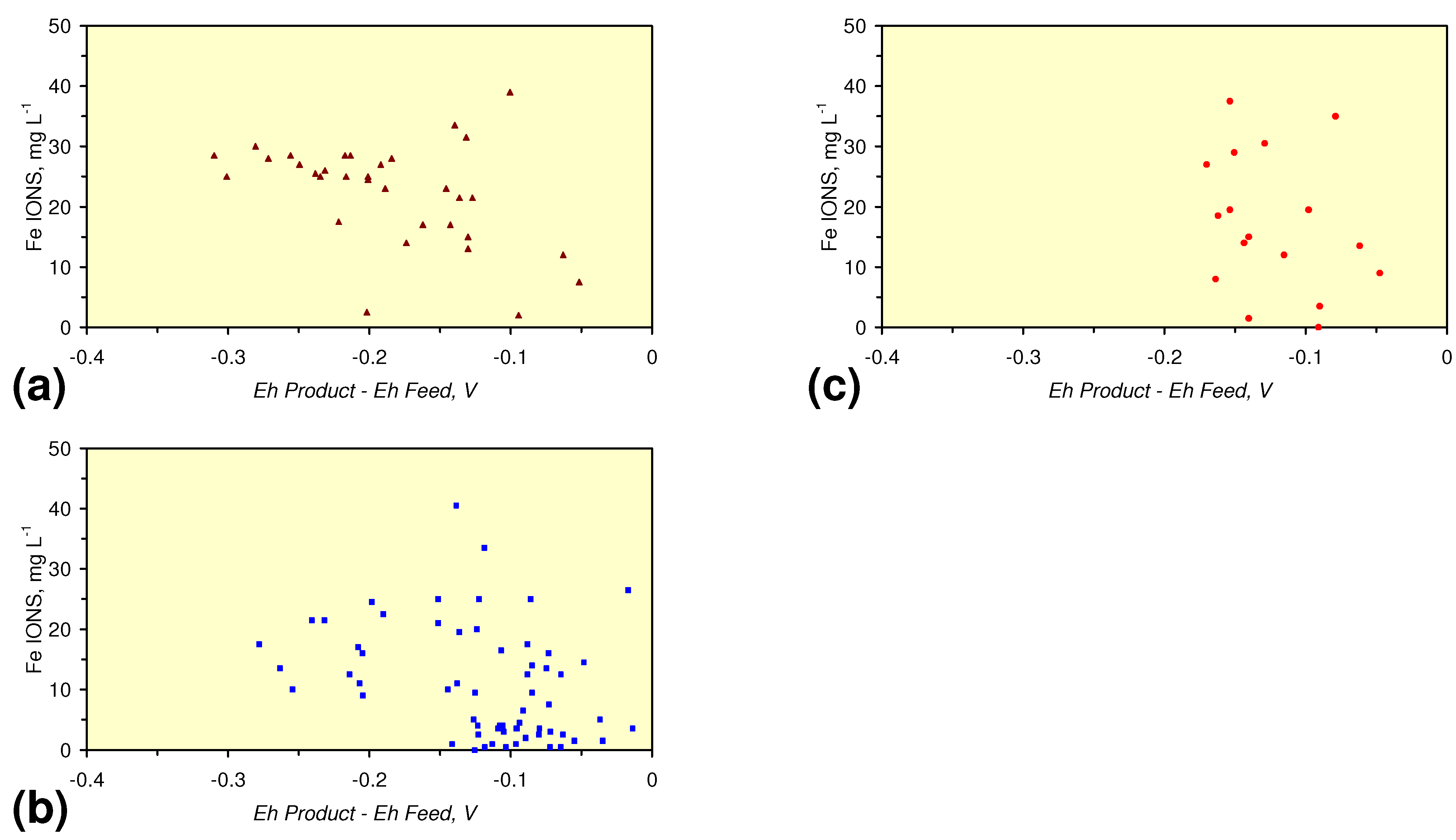
  • [EhproductEhFeed] becomes increasingly negative with decreasing SV until 1 < SV < 10, before becoming less negative when SV < 1 (Figure 32). The maximum observed decrease in Eh is between 0.3 and 0.4 V (Figure 32).
  • A general trend of [EhproductEhFeed] becoming increasingly negative with increasing [pHproductpHFeed] is present (Figure 33). This indicates that the chemical process of Eh reduction and pH increase is related.
  • The ECproduct:ECFeed ratio reaches a maximum value when the pHProduct:pHFeed ratio is about 1.1 (Figure 34). The ECProduct:ECFeed ratio decreases as 1.1 < pHProduct:pHFeed ratio > 1.1 (Figure 34).

3.3.1. BR1

Eh = −0.0105 × Log(SV) − 0.0444; R2 = 0.071;
pH = −0.058 × Log(SV) + 6.9393; R2 = 0.055;
EC:ECFeed = 0.111 × Log(SV) + 0.827; R2 = 0.36;

3.3.2. BR2

Eh = −0.0121 × Log(SV) − 0.0379; R2 = 0.072;
pH = −0.3385 × Log(SV) + 7.873; R2 = 0.23;
EC:ECFeed = 0.0058 × Log(SV) + 1.0441; R2 = 0.025;

3.3.3. BR3

Eh = 0.0058 × Log(SV) − 0.0798; R2 = 0.009;
pH = −0.0071 × Log(SV) + 6.7781; R2 = 0.001;
EC:ECFeed = −0.0127 × Log(SV) + 1.0944; R2 = 0.09;
The Feed Composition was Eh (mean = 0.137 V; SD = 0.042 V); pH (mean = 6.39; SD = 0.151); EC (mean = 0.278 mS cm−1; SD = 0.015 mS cm−1).
Figure 25. SV vs. pH: m-ZVM. (a) BR1 (n = 108; test duration = 74,380 min); (b) BR2 (n = 109; test duration = 74,560 min); (c) BR3 (n = 109; test duration = 74,560 min).
Sustainability 02 02988 g025
Figure 26. SV vs. Eh: m-ZVM. (a) BR1; (b) BR2; (c) BR3.
Sustainability 02 02988 g026
Figure 27. SV vs. EC:ECFeed: m-ZVM. (a) BR1; (b) BR2; (c) BR3.
Sustainability 02 02988 g027
Figure 28. Eh vs. pH: m-ZVM. (a) BR1; (b) BR2; (c) BR3; Feed water = blue triangles. Redox boundaries from [73].
Sustainability 02 02988 g028
Figure 29. EC:ECFeed Ratio vs. pH: m-ZVM. (a) BR1; (b) BR2; (c) BR3.
Sustainability 02 02988 g029
Figure 30. EC:ECFeed Ratio vs. Eh: m-ZVM. (a) BR1; (b) BR2; (c) BR3.
Sustainability 02 02988 g030
Figure 31. [pHProduct – pHFeed] vs. SV: m-ZVM. (a) BR1; (b) BR2; (c) BR3.
Sustainability 02 02988 g031
Figure 32. [EhProduct – EhFeed] vs. SV: m-ZVM. (a) BR1; (b) BR2; (c) BR3.
Sustainability 02 02988 g032
Figure 33. [EhProduct – EhFeed] vs. [pHProduct – pHFeed]: m-ZVM. (a) BR1; (b) BR2; (c) BR3.
Sustainability 02 02988 g033
Figure 34. [ECProduct:ECFeed] vs. [pHProduct:pHFeed]: m-ZVM. (a) BR1; (b) BR2; (c) BR3.
Sustainability 02 02988 g034

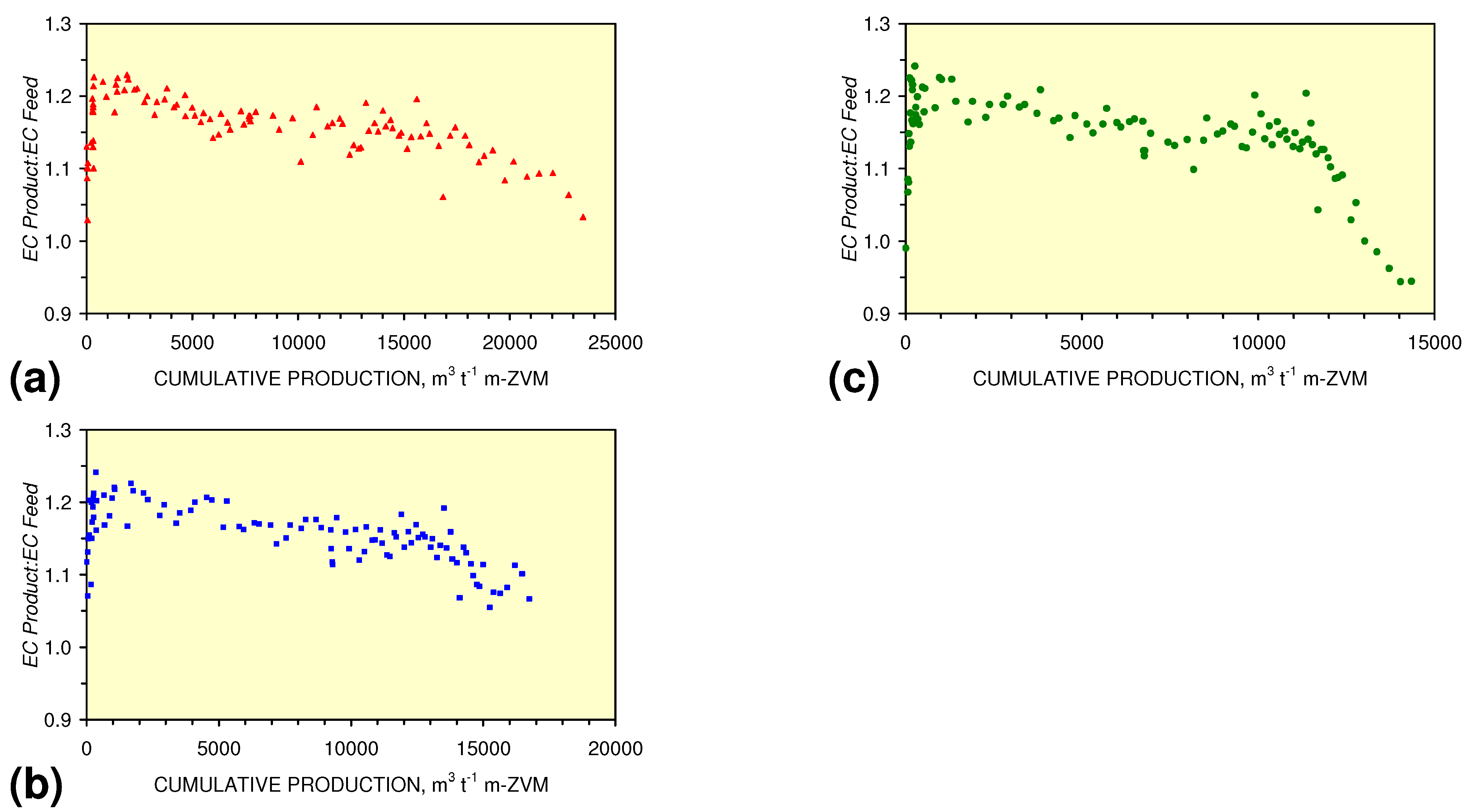
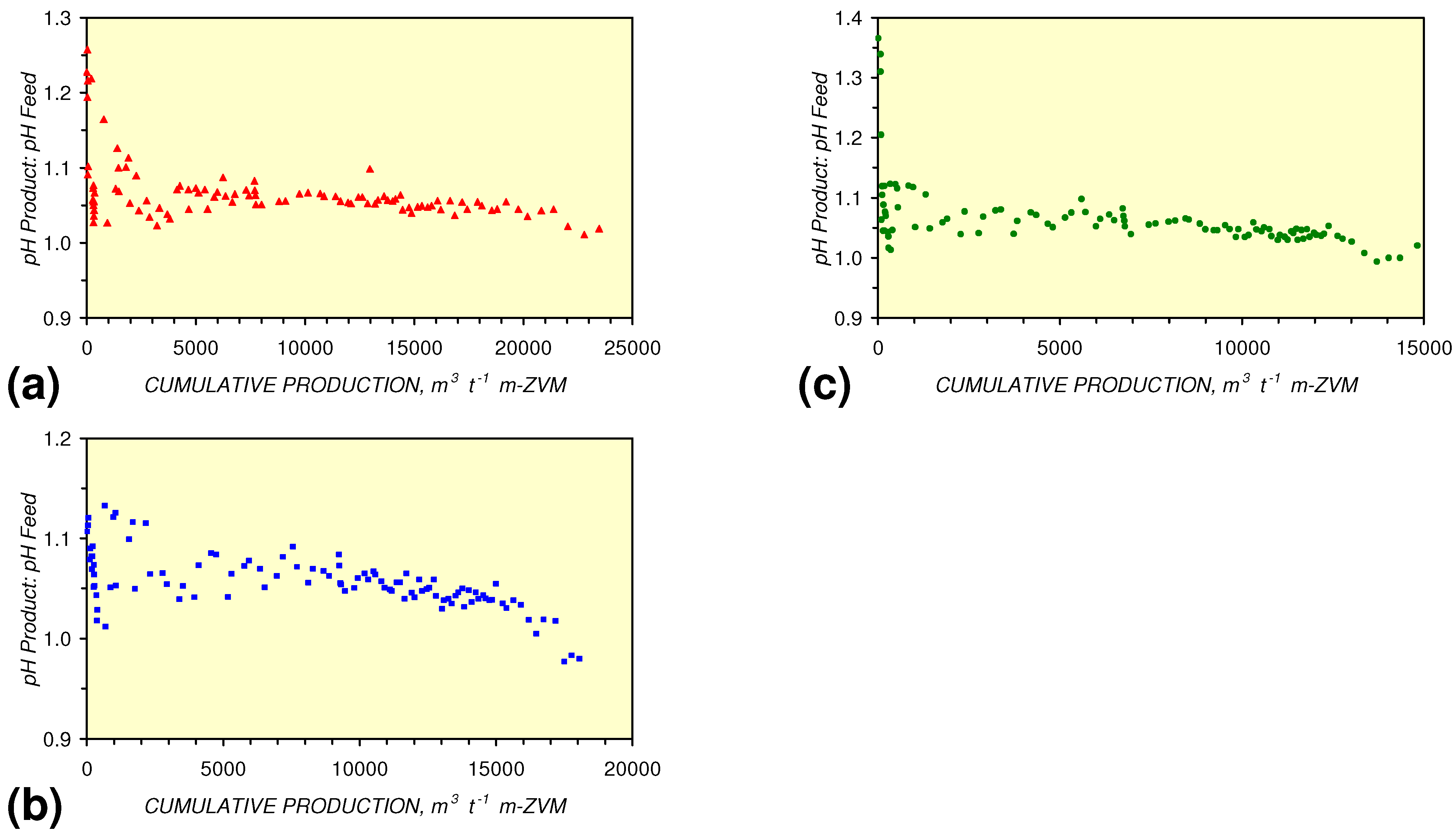
3.3.4. Cumulative Water Volume Processed

All ZVM treatments in a reactor have a finite life. This life expectancy varies with ZVM type and can be expressed in terms of cumulative processed water volume per unit weight of ZVM. The reactors showed a number of general trends:-
  • The ratio ECProduct:ECFeed decreased gradually with cumulative water volume processed (Figure 35). However, as the effectiveness of the ZVM decreased, the ratio decreased markedly (Figure 35).
  • [EhProductEhFeed] remained negative and constant with increasing cumulative processed water volume until the effectiveness of the ZVM decreased (Figure 36). [EhProductEhFeed] then decreased to zero with increasing cumulative processed water volume (Figure 36).
  • The ratio pHProduct:pHFeed and [pHproductpHFeed] decreased gradually with cumulative water volume processed (Figure 37 and Figure 38). However, as the effectiveness of the ZVM decreased, the ratio decreased markedly (Figure 37 and Figure 38).
  • m-Fe0 is able to process a larger volume of water (23,500 m3 t−1 m-Fe0) than either m-Fe0 + m-Cu0 (18,000 m3 t−1 m-Fe0 + m-Cu0) or m-Fe0 + m-Cu0 + m-Al0 (14,800 m3 t−1 m-Fe0 + m-Cu0) (Figure 35, Figure 36, Figure 37 and Figure 38).
The observed regression relationships between the relationship between cumulative water volume processed (Vc, m3 t−1 m-ZVM) and the ratios [pHProduct:pHFeed] and [ECProduct:ECFeed] are:
BR1: [pHProduct:pHFeed] = −1.9 × 10⁻⁶ × (Vc > 4, 000) + 1.0789; R2 = 0.476;
BR2: [pHproduct:pHFeed] = −4.1 × 10⁻⁶ × (Vc > 4,000) + 1.0976; R2 = 0.633;
BR3: [pHProduct:pHFeed] = −4.8 × 10−6 × (12,000 > Vc > 4,000) + 1.0944; R2 = 0.583;
[pHProduct:pHFeed] = −2.26 × 10−5 × (12,000 > Vc > 4,000) + 1.3167; R2 = 0.843;
BR1: [ECProduct:ECFeed] = −2.8 × 10−6 × (17,000 > Vc >4000) + 1.189; R2 = 0.233;
[ECProduct:ECFeed] = −1.56 × 10⁻⁵ × (Vc > 17,000) + 1.4171; R2 = 0.856;
BR2: [ECProduct:ECFeed] = −4.8 × 10−6 × (13,000 > Vc > 4,000) + 1.2028; R2 = 0.317;
[ECProduct:ECFeed] = −4.4 × 10⁻⁶ × (Vc > 13,000) + 1.599; R2 = 0.004;
BR3: [ECProduct:ECFeed] = −37 × 106 × (12,000 > Vc > 4,000) + 1.1779; R2 = 0.115;
[ECProduct:ECFeed] = −7.6 × 10−5 × (12,000 > Vc > 4,000) + 2.0096; R2 = 0.974;
BR1: [EhProductEhFeed] = 8 × 10⁻⁷ × (Vc > 4,000) – 0.227; R2 = 0.02;
BR2: [EhProduct EhFeed] = 3.6 × 10⁻⁶ × (Vc > 4,000) − 0.2492; R2 = 0.159;
BR3: [EhProduct:EhFeed] = 3.0 × 10−6 × (12,000 > Vc > 4,000) − 0.2433; R2 = 0.091;
[EhProduct:EhFeed] = 4.3 × 10⁻⁵ × (Vc > 12,000) − 0.7098; R2 = 0.5;
Figure 35. [ECProduct:ECFeed] vs. Cumulative Feed: m-ZVM. (a) BR1; (b) BR2; (c) BR3.
Sustainability 02 02988 g035
Figure 36. [EhProduct – Eh Feed] vs. Cumulative Feed: m-ZVM. (a) BR1; (b) BR2; (c) BR3.
Sustainability 02 02988 g036
Figure 37. [pHProduct:pHFeed] vs. Cumulative Feed: m-ZVM. (a) BR1; (b) BR2; (c) BR3.
Sustainability 02 02988 g037
Figure 38. [pHProduct:pHFeed] vs. Cumulative Feed: m-ZVM. (a) BR1; (b) BR2; (c) BR3.
Sustainability 02 02988 g038

4. Discussion/Implications/Applications

4.1. Fe Ion Type

The changes in Eh and pH are associated with the formation of different types of Fe ions and their interaction with water, OxH ions and the hydronium ion.
The hydronium ion is variously expressed as:
  • H3O+(H2O)n, n = 1–3 [74,75],
  • H3O+(H)n, n = 1–3, H2O − H+ − OH2 [75],
  • hydrated H+ ions [(H9O4+) [76]], H+(H2O)n, n = 1–28 [75] and
  • H3O+(X)n where X = H2, N2, CO, and n = 0 −> 3 [77].
The interaction of Fe and HnOy is complex but results in the formation of three generic groups of ion types:
  • Fen+(aq) [73],
  • FeOH+(aq) [73], and
  • Fe(a−n)+-Hn(aq), a = 2,3; where Fe(a−n)+-Hn(aq) includes Fea+-H3O(H2)n(aq), Fe-H+, Fe-(H2)+, Fe(a−n)+(Y)n(aq) and Fea+-H3O(X,Y)n(aq). Y = H2, H2O, COx, CxHy, CxHyOz, etc., e.g., [29,32].
The formation of Fe2+(aq) leaves pH and Eh unchanged, e.g.,
Fe0 = Fen+(aq)
The formation of FeOH+(aq) reduces pH and increases Eh by removing OH, e.g.,
Fe0 + OH = FeOH+(aq)
This reaction increases the H3O+:[OH+ HO2] ratio (i.e., decreases pH), and reduces the OH:HO2 ratio (i.e., increases Eh). The formation of Fe(a−n)+Hn(aq) increases pH (by removing H3O+) and decreases Eh (by increasing the OH:HO2ratio), e.g.,
FeO + 2HO2− + 2H3O+ = Fe-(H2)+(aq) + 6OH
or increases pH, but leaves Eh unchanged by removing H3O+, e.g.,
FeO + H3O+ = Fe-(H)+(aq) + H2O
or increases pH, and decreases Eh by increasing the [OH + HO2]: H3O+ ratio and increasing the OH:HO2 ratio, e.g.,
FeO + 2H2O = Fe-(H2)+(aq) + 2OH
Equation 58 is sometimes stated [4,78] as:-
Fe0 + 2H2O = Fe2+ + H2(g) + 2OH
The formation of Fe-(H2)+(aq) from FeOH+ can be associated with a decrease in pH, an increase in Eh and the formation of O2(g), e.g.,
2FeOH+(aq) + 2OH= 2Fe-(H2)+(aq) + O2(g)
or a decrease in pH and a decrease in Eh, e.g.,
FeOH+ + HO2 = Fe-(H2)+(aq) + 1.5O2(g)
The formation of Fe-(H)+(aq) from Fe2+ and Fe3+ ions can be associated with a decrease in pH, a decrease in Eh and the formation of O2(g), e.g.,
Fe2+ + HO2 = Fe-(H)+(aq) + O2(g)
Fe2+ + OH = Fe-(H)+(aq) + 0.5O2(g)
Fe3+ + 2OH = Fe-(H2)+(aq) + O2(g)
O2(g) can form from the reduction of OxH by Fe0, decreasing pH and increasing Eh, e.g.,
Fe0 + 2OH = Fe-(H2)+(aq) + O2(g)
or decreasing pH and decreasing Eh, e.g.,
Fe0 + HO2 = Fe-(H)+(aq) + O2(g)
Reduction of [Fe0 + OxH], [FeOH+(aq) + OxH] and [Fea+ + OxH] to form Fe(a−n)+Hn(aq) is the principal reason why O2(g) bubbles (and associated macropore/gas venting structures) are observed in ZVM beds. The reduction by [Fe0 + OxH], is accelerated by the addition of Al0, or Cu0 + Al0. The principal iron redox stability zones (Figure 39) indicate that the observed O2 degassing (from m-ZVM) primarily relates to activity while the water redox environment is within the Fe2+(aq) and FeOH+(aq) stability zones (Equations 60–63) and from the Fe0 bed (Equations 65, 66). In n-ZVM the O2(g) degassing relates to activity while the redox environment is within the FeOH+(aq), Fe2O3(s) and Fe3O4(s) stability zones (Figure 39).
Figure 39. Fe Redox environment. (a) Redox boundaries from [73]. (b) Redox environment associated with O2(g) release in Figure 5, Figure 6, Figure 7, Figure 8, Figure 9, Figure 10, Figure 40, Figure 41, Figure 46 and Figure 70.
Sustainability 02 02988 g039

4.1.1. Permeability Implications

In the static diffusion reactors, the water Eh-pH changes with decreasing SV into the hematite (Fe2O3) stability zone (Figure 39). In this environment limonite crusts (FeO(OH)nH2O) are observed to form at the ZVM-water interface when only n-Fe0 is present (Figure 7) or at the mouth of O2(g) discharge conduits when n-Fe0 + n-Cu0 are present (Figure 7). Limonite is absent at the mouth of O2(g) discharge conduits when Fe0 + Al0, or Fe0 + Cu0 + Al0 are present (Figure 9). The limonite is considered to form as:
Fe+H(aq) + O2(g) + nH2O = FeO(OH)nH2O(s)
The permeability (Figure 3) of the n-Fe0 + n-Cu0 + n-Al0 bed remains relatively constant with time. The permeability of n-Fe0 and n-Fe0 + nCu0 decreases with time where the rate of permeability decrease is greater in n-Fe0 bed than n-Fe0 + n-Cu0 bed. The experimental observations (e.g., Figure 7) indicate that Equation 67 is favored by high contact/residence times between Fe+-H(aq) + O2(g)at the ZVM-water interface. Increasing the ratio of Fe(a−n)+-H(aq):O2(g) at the ZVM-water interface (resulting from decreasing permeability) will favor limonite production. Limonite production will block macropores, requiring the development of a fractured surface (Figure 7) to allow O2(g) to escape from the n-Fe0 bed. The continuous flow reactors and static diffusion reactor analyses indicate that significantly higher Fe ion formation is associated with m/n-Fe0 than with m/n-Fe0 + m/n-Cu0 and m/n-Fe0 + m/n-Cu0 + m/n-Al0.
Figure 40. n-Fe0 + n-Cu0 + n-Al0(a) Structure of n-ZVM bed after 72 hours when Ca-montmorillonite is present. The n-Fe0 forms a crystalline zone containing trapped O2 bubbles (associated with n-Al0) and macropore/fractures. A buried n-Cu0 ejection vent is present (top left). Field of view = 30 mm. Eh = −0.286 V; pH = 9.21; EC = 0.734 mS cm−1; T = 24.1 °C; Freshwater feed Eh = 0.164 V; pH = 6.42; EC = 0.253 mS cm−1. ZVM bed weight ratio 7.7 Ca-montmorillonite: 6.5 n-Fe0: 1.67 n-Al0: 1 n-Cu0. (b) Cross-section (4 mm thickness) through stratified n-ZVM after 76 days showing Cu oxides (green) overlain by n-Cu0 (copper), n-Al0 (light grey) and crystalline Fe0(dark grey)/goethite nodules (red-brown/black). The crystalline layers are overlain by a layer of n-Fe0/n-Al0. Ca-montmorillonite is absent. Eh = −0.171 V; pH = 9.26; EC = 0.152 mS cm−1; T = 12.1 °C; Freshwater Feed: Eh = 0.032 V; pH = 7.12; EC = 0.347 mS cm−1. ZVM bed weight ratio 6.5 n-Fe0: 1.67 n-Al0: 1 n-Cu0; (c) Cross-section (10 mm thickness) through stratified n-ZVM after 98 days showing n-Al diapirism, clod-macropore arrangement at the n-ZVM-water interface, The n-Fe0 is starting to show a crystalline structure. Ca-montmorillonite is absent. Eh = −0.080 V; pH = 8.74; EC = 0.183 mS cm−1; T = 16.6 °C; ZVM bed weight ratio 6.5 n-Fe0: 1.67 n-Al0:1 n-Cu0
Sustainability 02 02988 g040
Figure 41. n-Fe0 + n-Cu0 + n-Al0. (a) Saline water: graded n-ZVM bed (from water-n-ZVM contact, to copper rich basal layer). 39 days after n-ZVM bed formation. Stratification is formed by O2 ejection. n-Al0 diapiric structures are present. Vertical streamers in the n-ZVM bed indicate n-O2(g) discharge routes from the n-Cu0 rich layer. Similar streamers have been observed when air is expelled from clay. Vertical column is 15 mm. Eh = −0.288 V; pH = 8.37; EC = 2.000 mS cm–1; T = 20.0 °C; ZVM bed weight ratio 7.7 Ca-montmorillonite:6.5 n-Fe0: 1.67 n-Al0: 1 n-Cu0. Saline water feed: Eh = 0.147 V; pH = 6.27; EC = 1.836 mS cm−1. (b) Freshwater: Cross-section (5 mm thickness) through n-ZVM after 76 days showing Cu oxides overlain by n-Cu0, n-Al0, crystalline Fe0/goethite nodules under a layer on n-Fe0 (containing O2 bubbles). The n-Fe0 is overlain by water. (c) Enlargement of O2(g) bubble (bottom left Figure 40c) showing growth from the n-Al0 diapir into a natural fracture zone/natural pipe zone extending into a matrix which is dominantly n-Fe0.
Sustainability 02 02988 g041
Cross sections through n-ZVM beds containing n-Fe0 + n-Cu0 + n-Al0 indicate
  • the development of crystalline n-Fe0 structures when Ca-montmorillonite is present within a few days of bed formation (Figure 40a). Crystalline n-Fe0 is observed in the n-Fe0 + n-Cu0 + n-Al0 when Ca-montmorillonite is absent after about 50–70 days (Figure 40b, c).
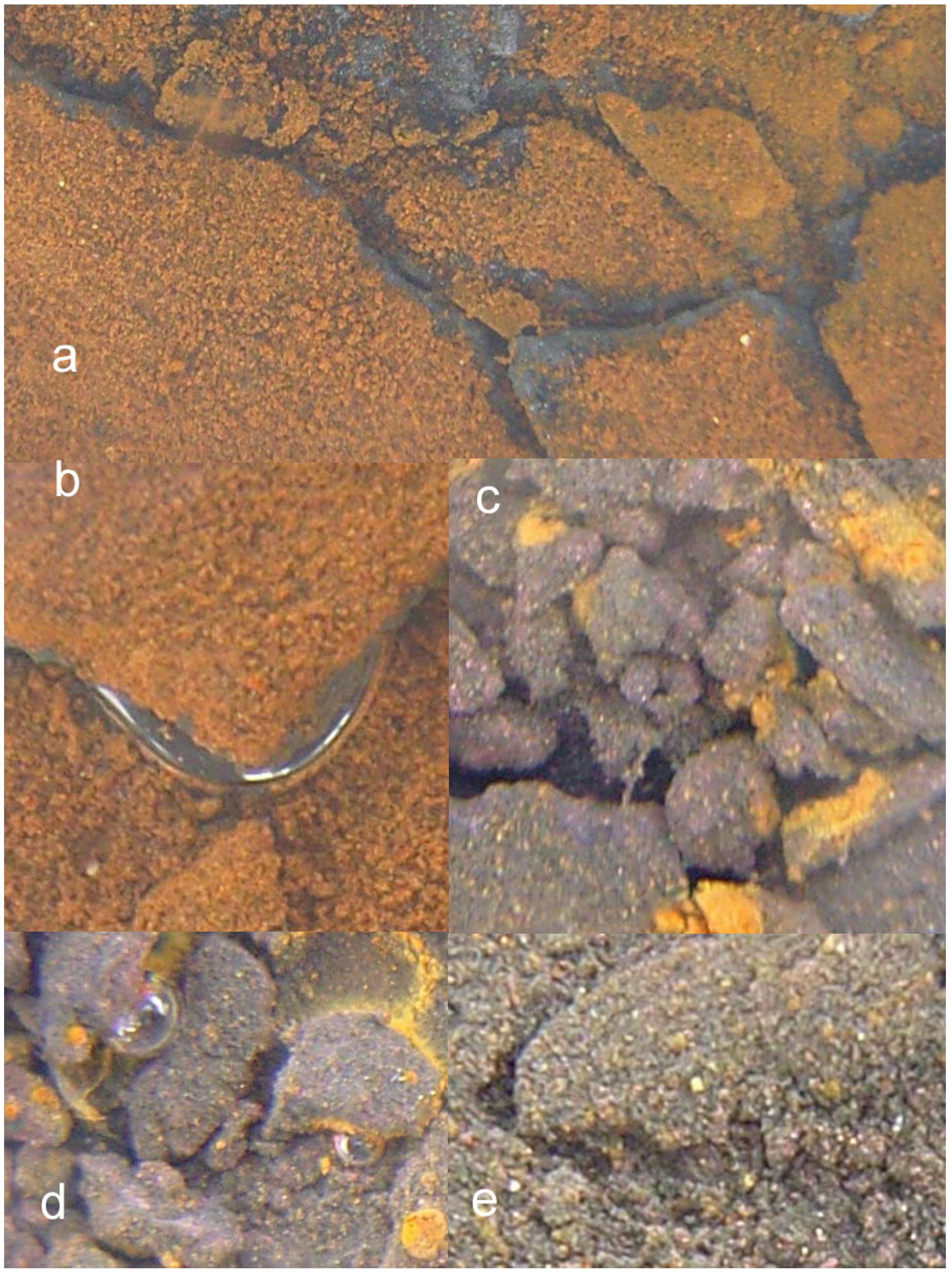
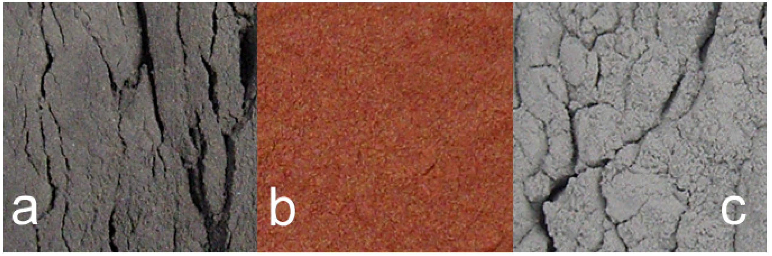
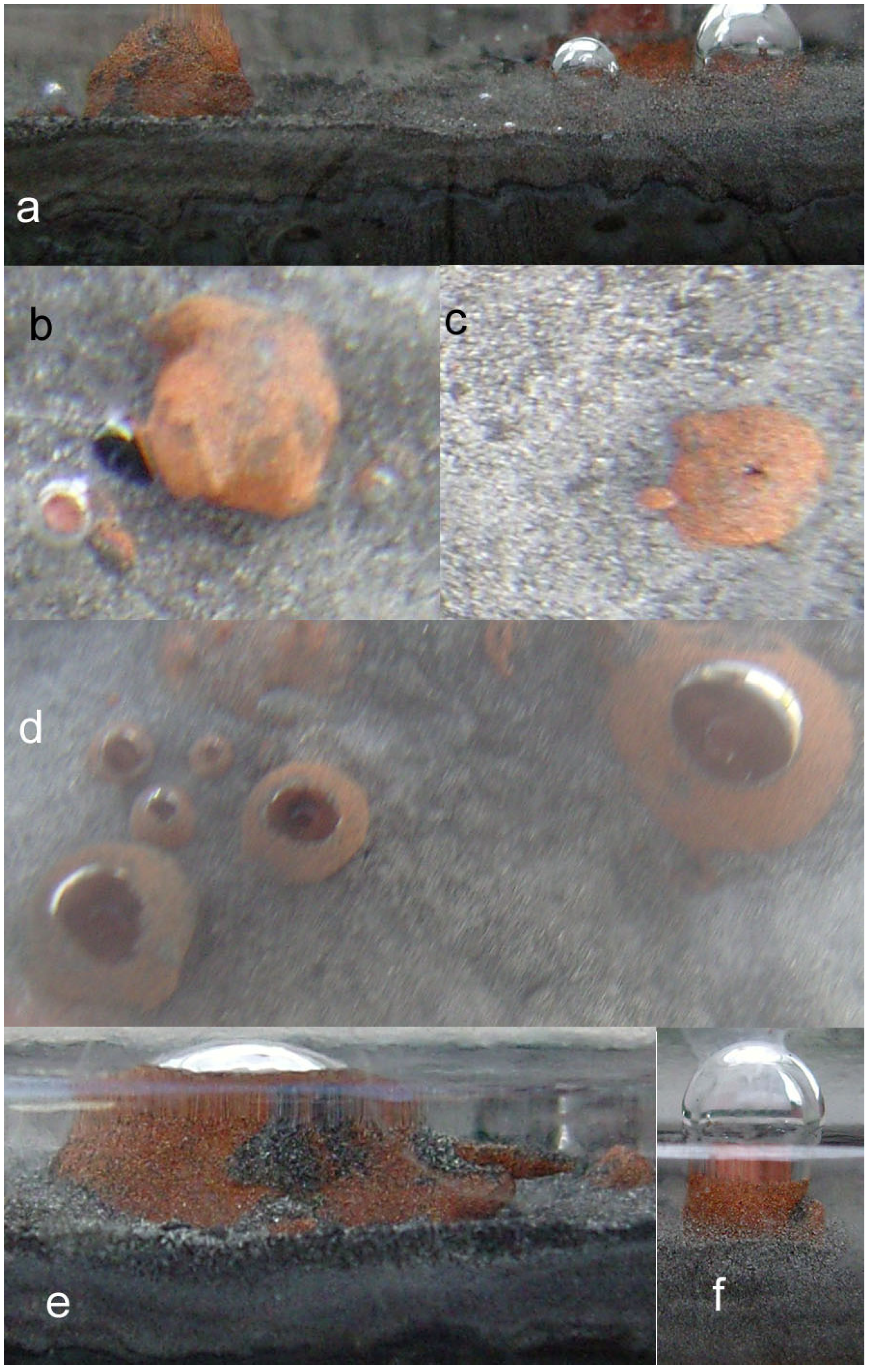
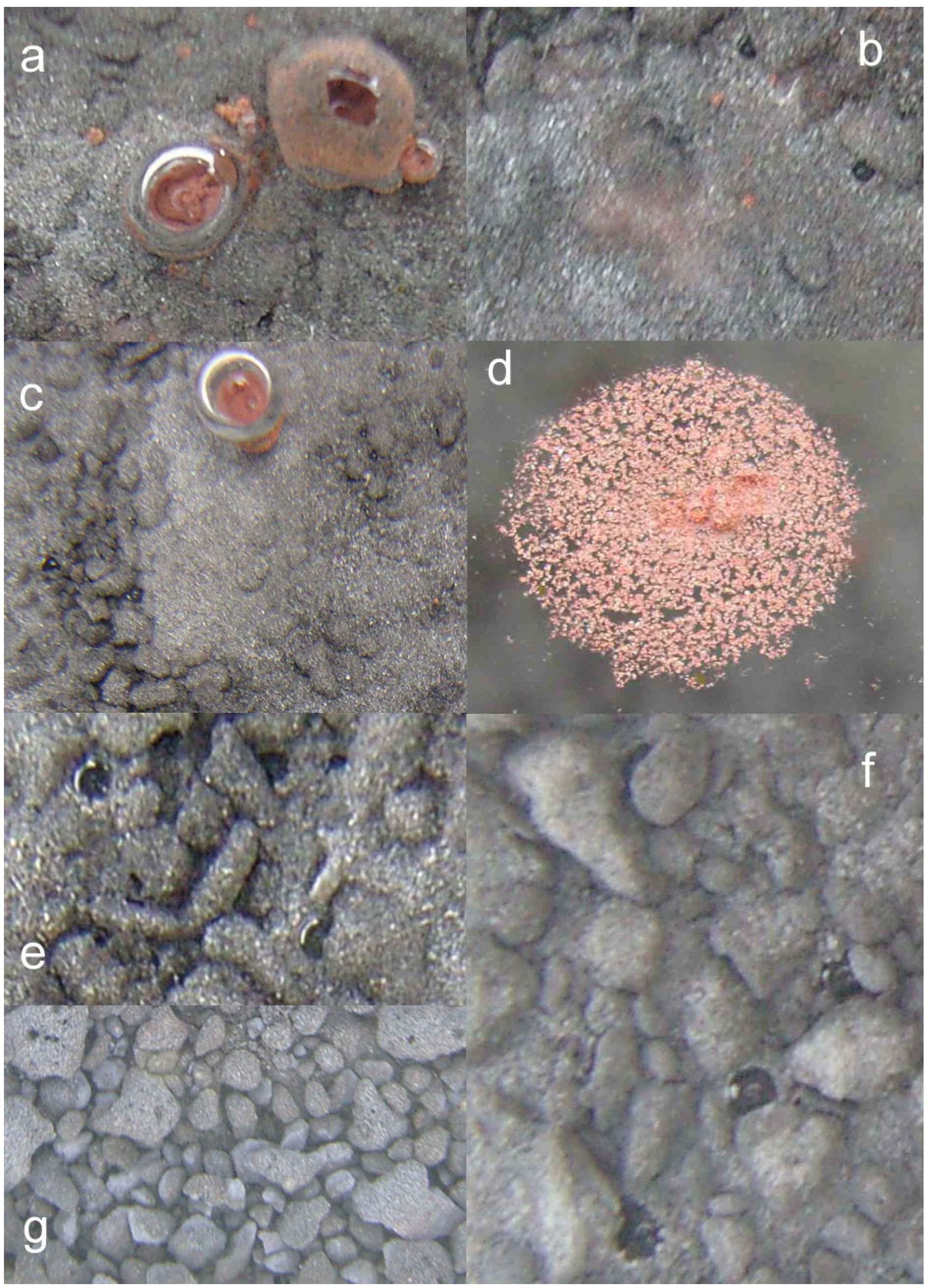
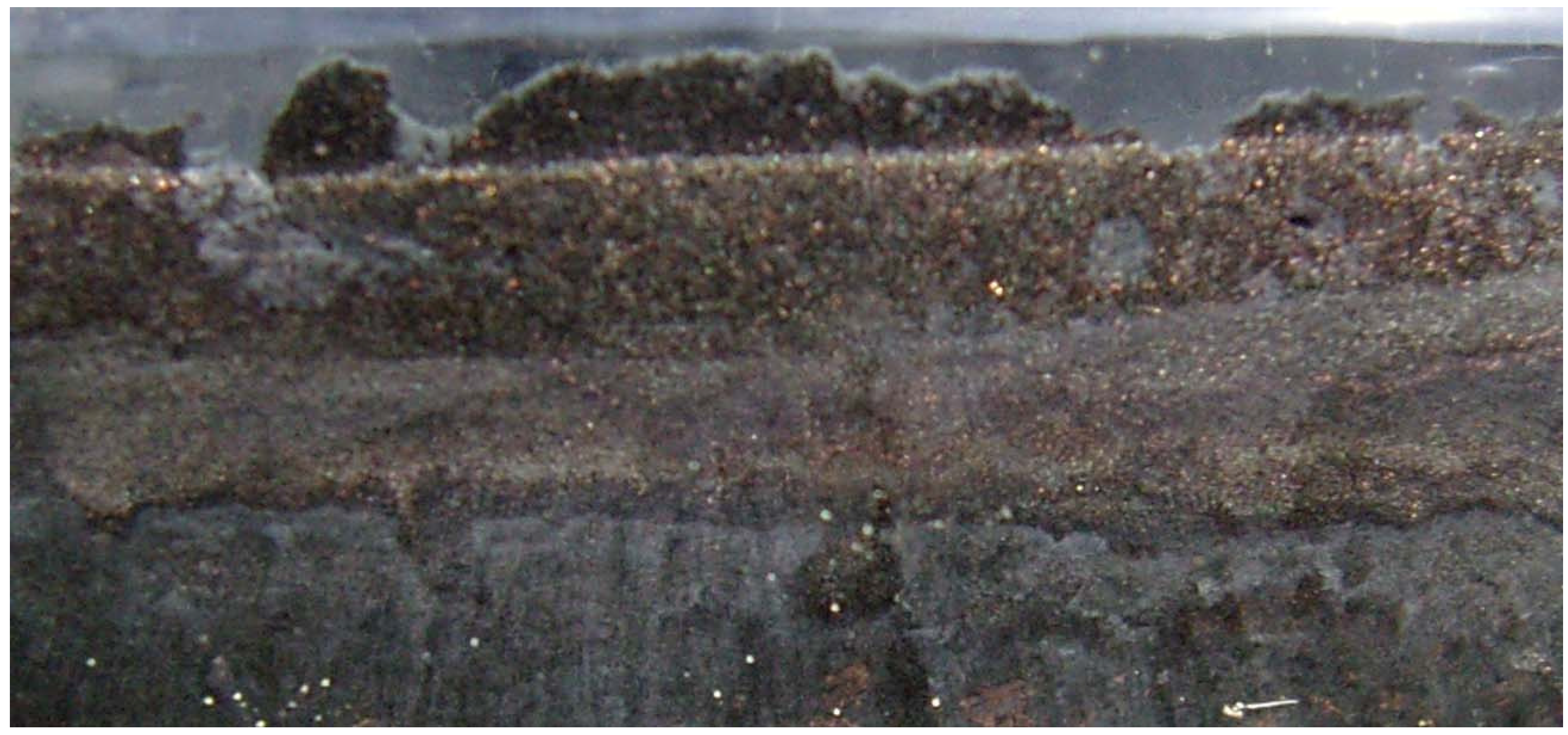
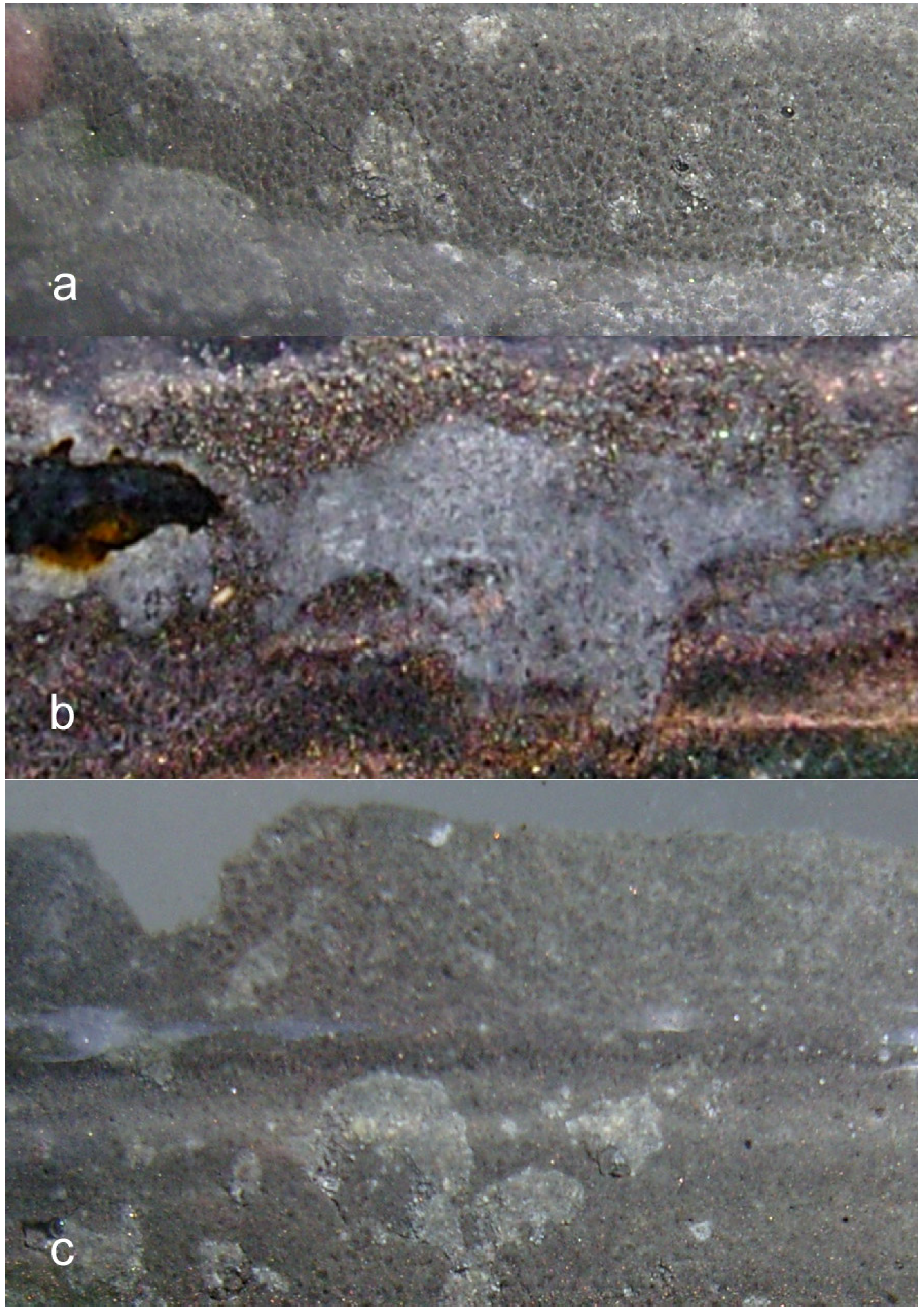
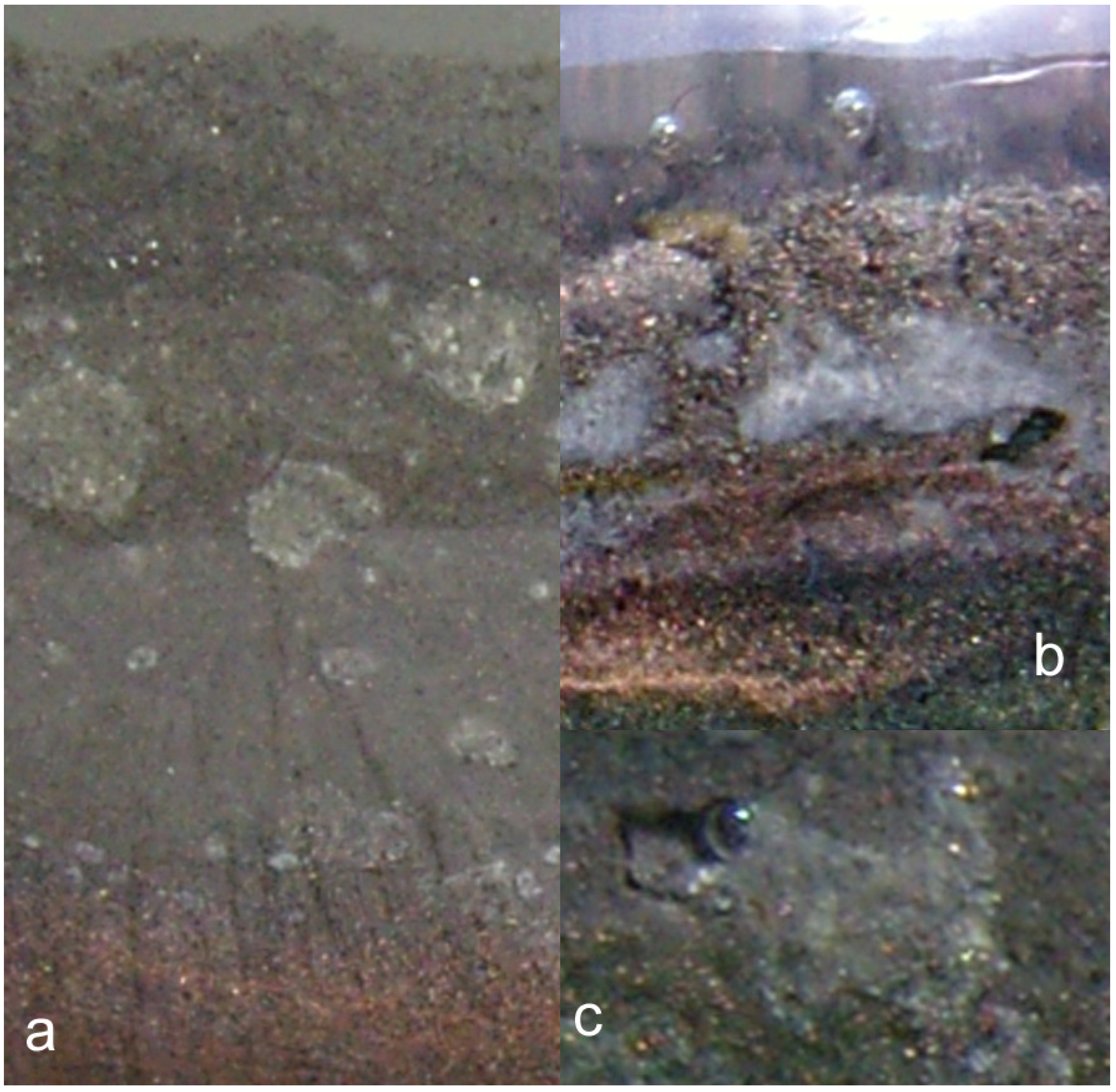
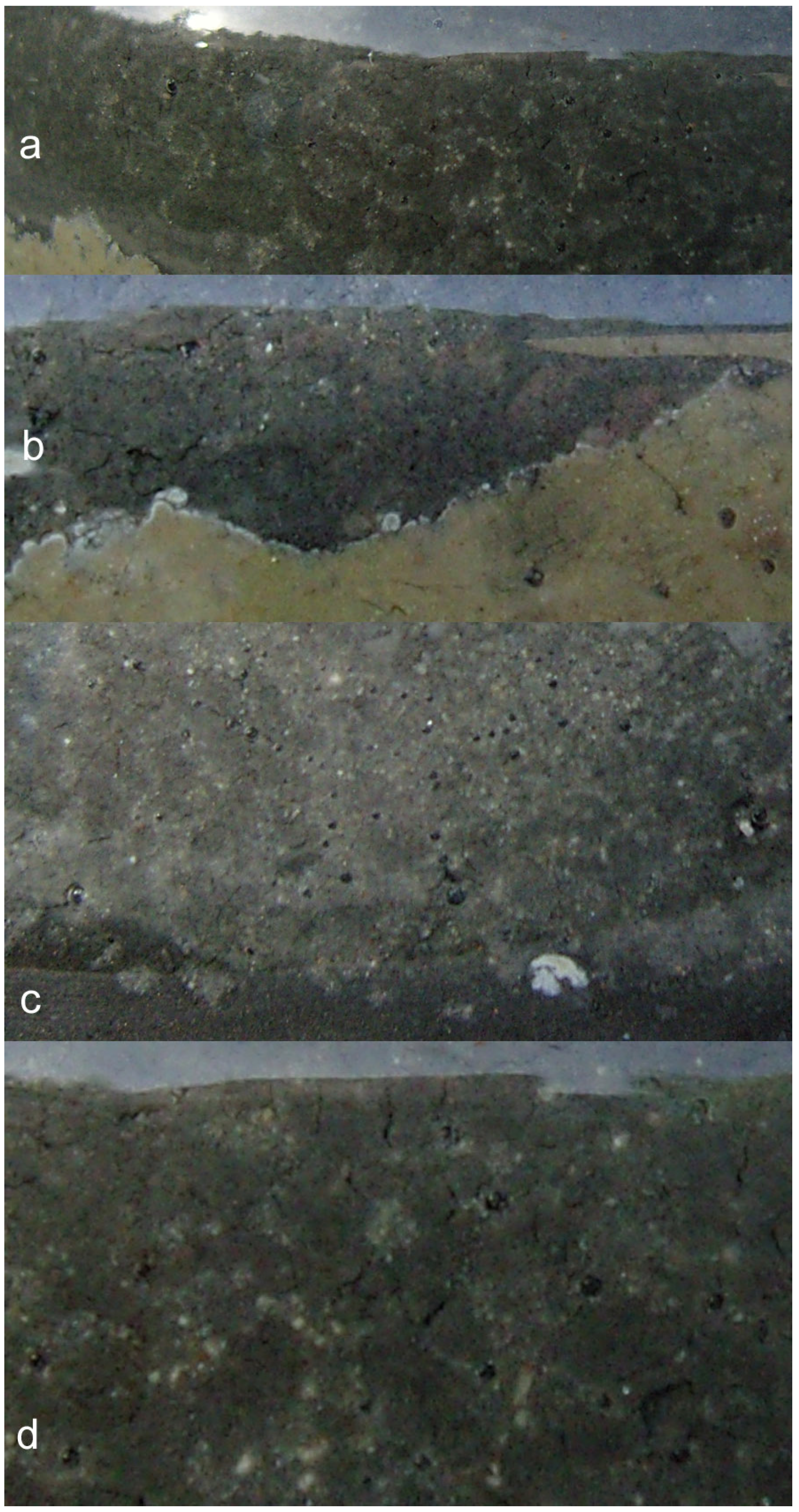
  • extensive development of goethite within the ZVM bed and extensive n-Al0 diapirism (Figure 40b).
  • raised particulate clod surfaces can be directly related to underlying n-Al0 diapirism (Figure 40c). Cracks within the n-Fe0 bed can be directly linked to the adjacent n-Al0 diapirs (Figure 40a, c). O2 gas bubbles are present within the n-Fe0 layers (Figure 40a, c and Figure 41), while the goethite is restricted to layers where n-Al0 and n-Fe0 are in contact (Figure 40 and Figure 41).
  • The active venting associated with O2 discharge results in the ZVM bed becoming density graded with concentrations of n-Al0 confined to diapiric structures (Figure 41a, b). Active O2(g) formation occurs in the vugs and macropores radiating from the n-Al0 diapirs (Figure 41c). The resulting gas bubbles rise through the crystalline n-ZVM bed into the amorphous n-ZVM bed immediately under the n-ZVM-water contact before discharging into the water (Figure 41b).
These crystalline changes provide an explanation as to why the permeability in the n-ZVM continuous flow reactors (DR1−DR2) declined with time while the permeability of DR3 while low, remained constant. i.e., the permeability decline in DR1 and DR2 is dominantly due to limonite precipitation at the water-ZVM interface which is associated with the interaction of the high level of Fe ion discharge and O2(g) discharge. The constant permeability in DR3 is a direct result of O2(g) discharge creating an interlinked network of macropores and vertical pipes/macropores providing a direct discharge route through the n-ZVM bed (Figure 41a).

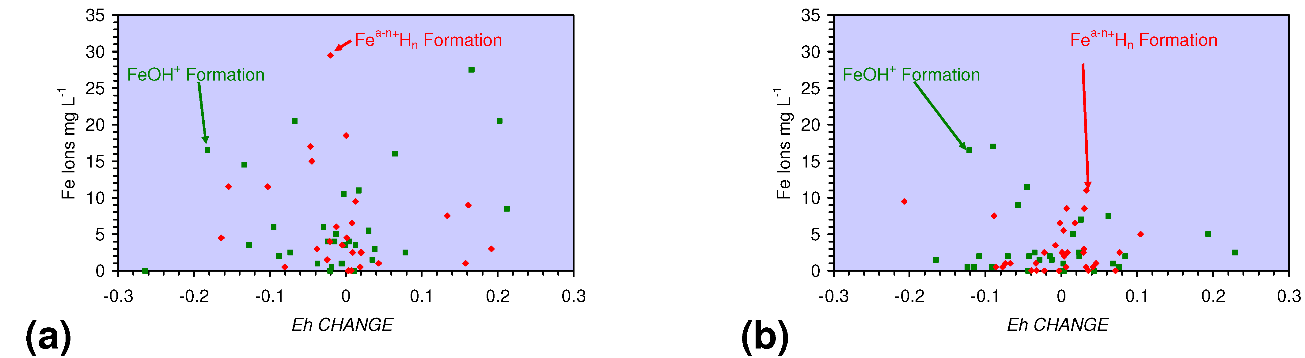
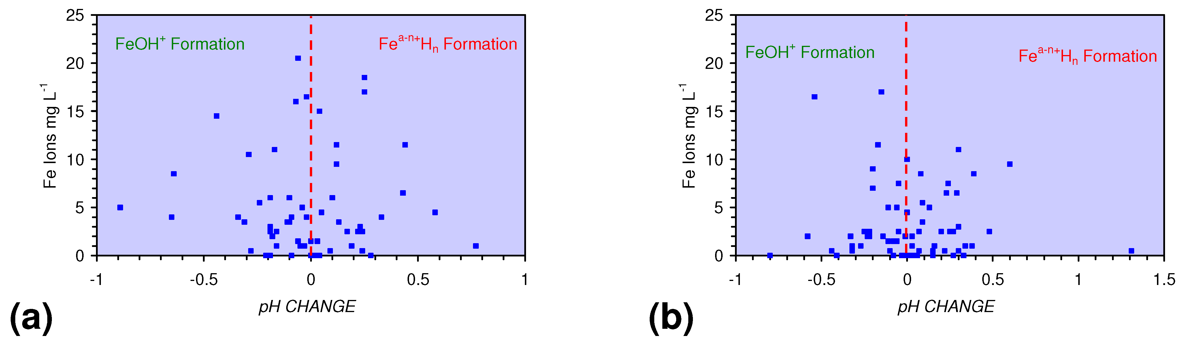
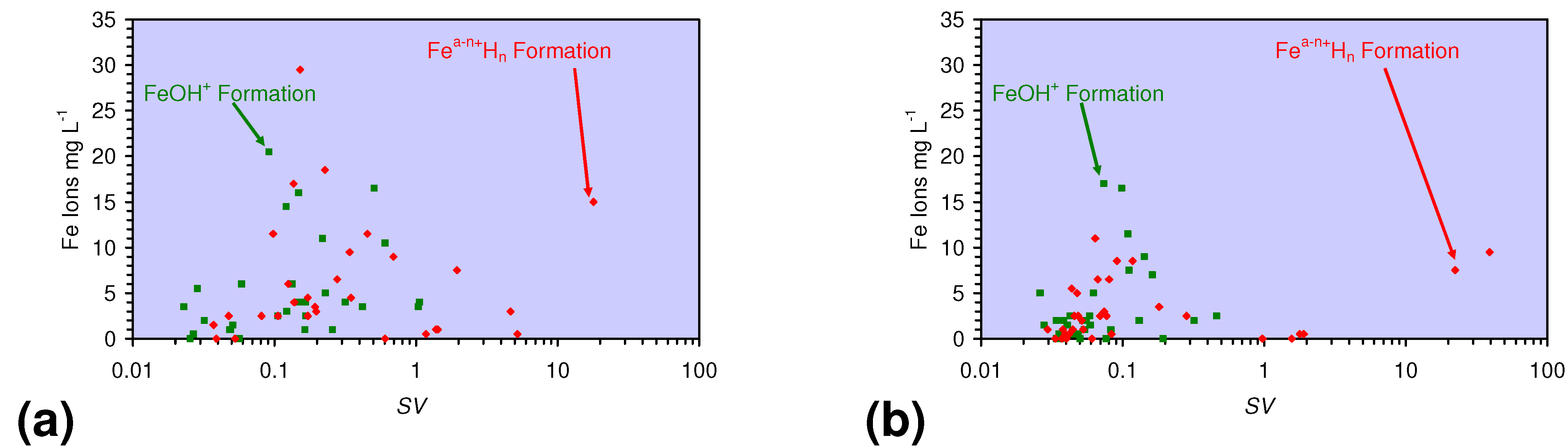
4.1.2. Remediation Implication of Fe Ion Type

The Fe(a−n)+-Hn(aq) and Fe(a−n)+-Hn(s) ions, when present, will act as active catalytic sites which will allow reduction of CxHyCln to CvHm, reduction of COx and CbHkOp to CnHm and CxHmOz, and polymerization of CxHy (or CxHyOz) to Cx+aHy+b and Cx+aHy+bOz+c [29,30,31,32]. The experimental results indicate that EC increases (i.e., Fe ion formation) are associated with
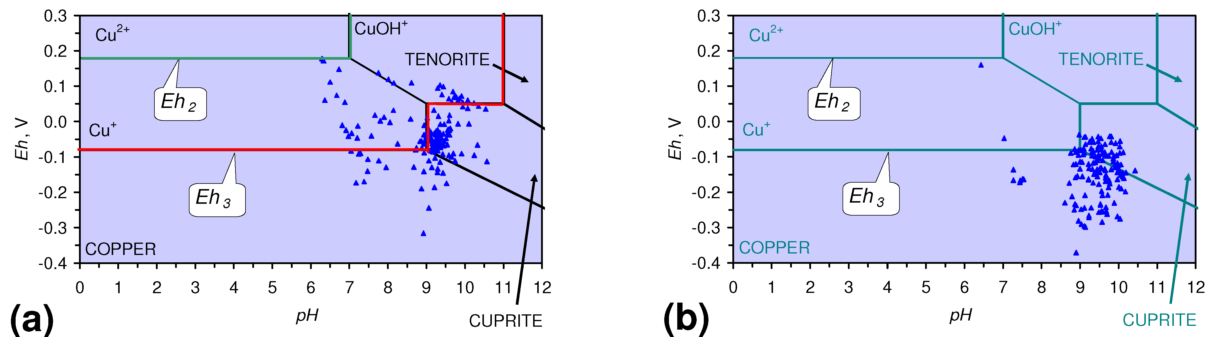
  • decreases in pH and increases in Eh (interpreted as indicating FeOH+(aq) formation), or,
  • increases in pH associated with increases or decreases in Eh (interpreted as indicating Fe(a−n)+H(aq) formation).
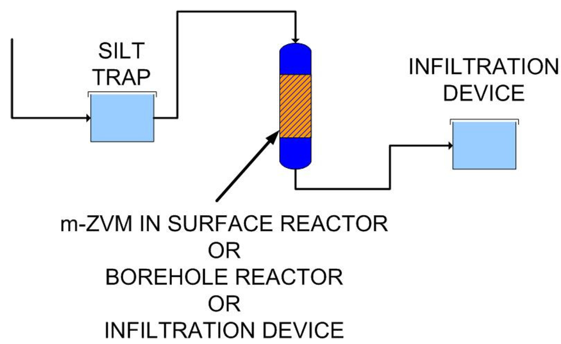
Much of the FeOH+ formation interpreted by this approach may actually represent Fe(a−n)+H(aq) formed from FeOH+(aq) and Fen+(aq) (i.e., Fe(a−n)+H(aq) formation will be underestimated).
In the borehole reactors, Fe ion formation occurs when the bulk of the product water is in the Fe2+ stability zone (Figure 39). However, Fe2+ formation cannot explain the observed associated Eh and pH changes. These indicate that the dominant ion type formed in the product water is Fe(a−n)+Hn(aq). Ion formation of 15–35 mg L−1 is associated with Eh reductions of 0.15 to 0.3 V (Figure 42) and a pH increase of 0.25 to 0.75 (Figure 43). Treatment of water with m-ZVM prior to entering the aquifer will therefore allow a high concentration of catalytically active Fe(a−n)+H(aq) to be delivered into the aquifer. This may significantly enhance the catalytic removal of contaminants within the aquifer. Comparison of these results (Figure 42 and Figure 43) with the equivalent results from the n-ZVM reactor (Figure 44 and ) indicates a similar pattern of Fe(a−n)+H(aq) ion formation
These observations indicate that aquifer remediation processes which rely on Fe(a−n)+H(aq), as a soluble catalyst, can be enhanced by
3.
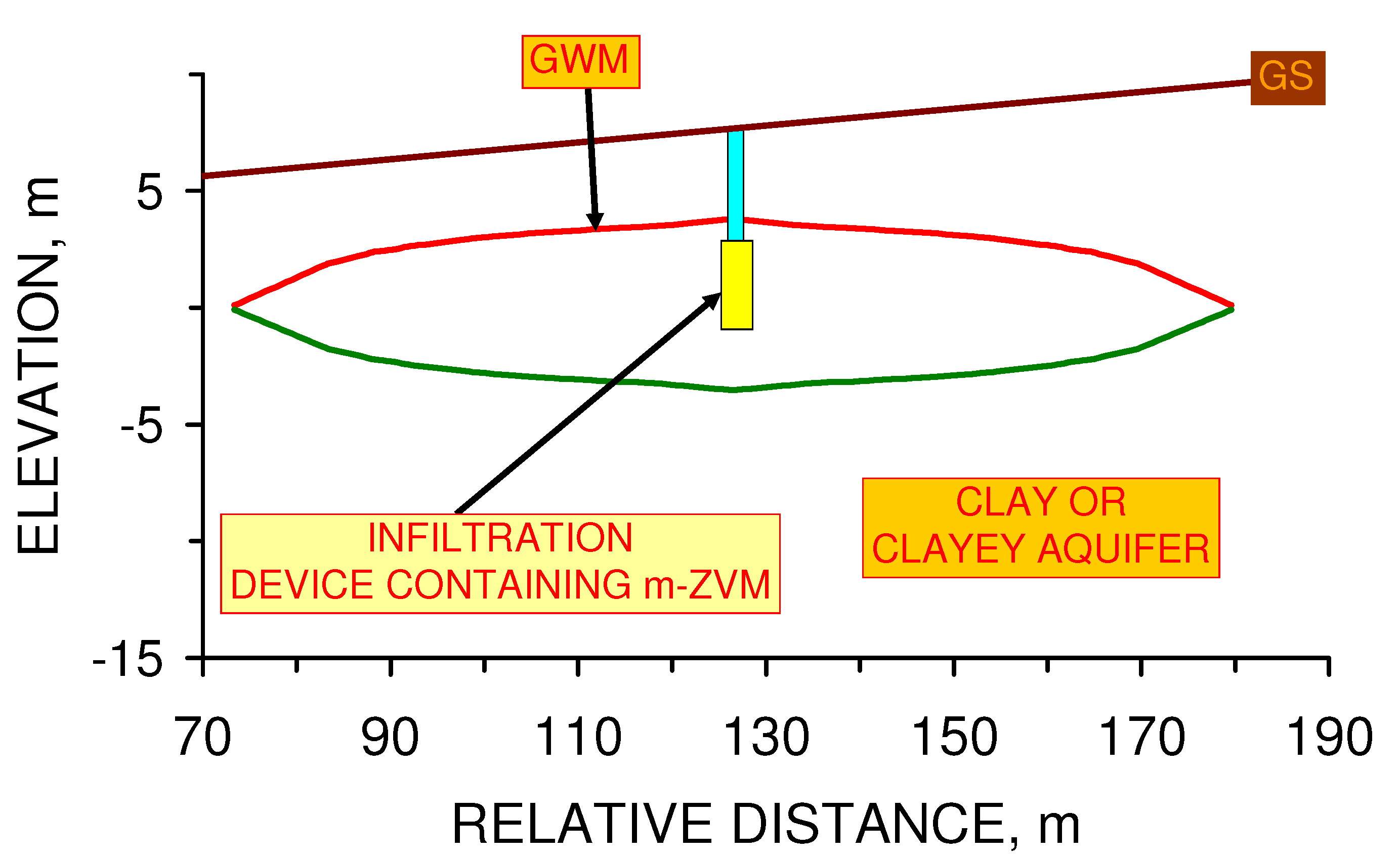
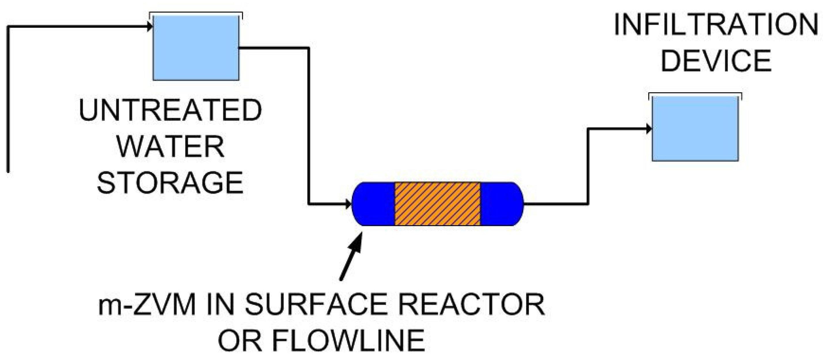
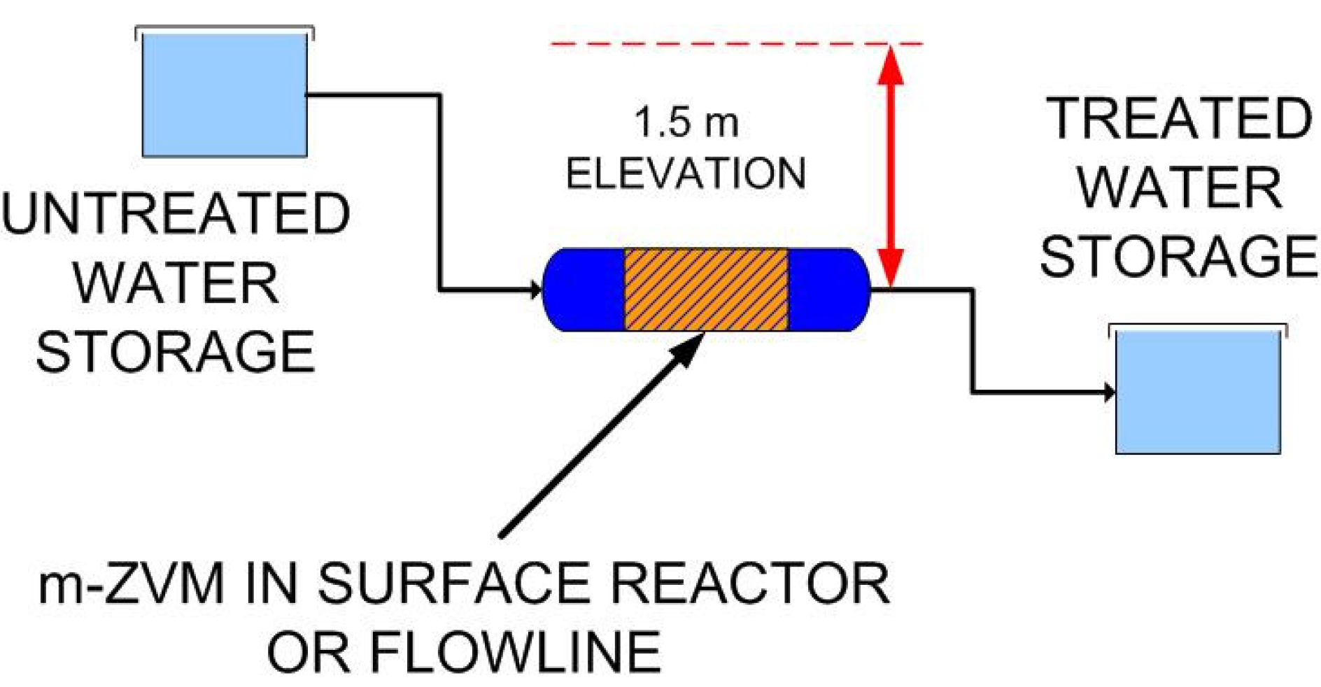
passing infiltrating water through m-ZVM prior to entering the aquifer,
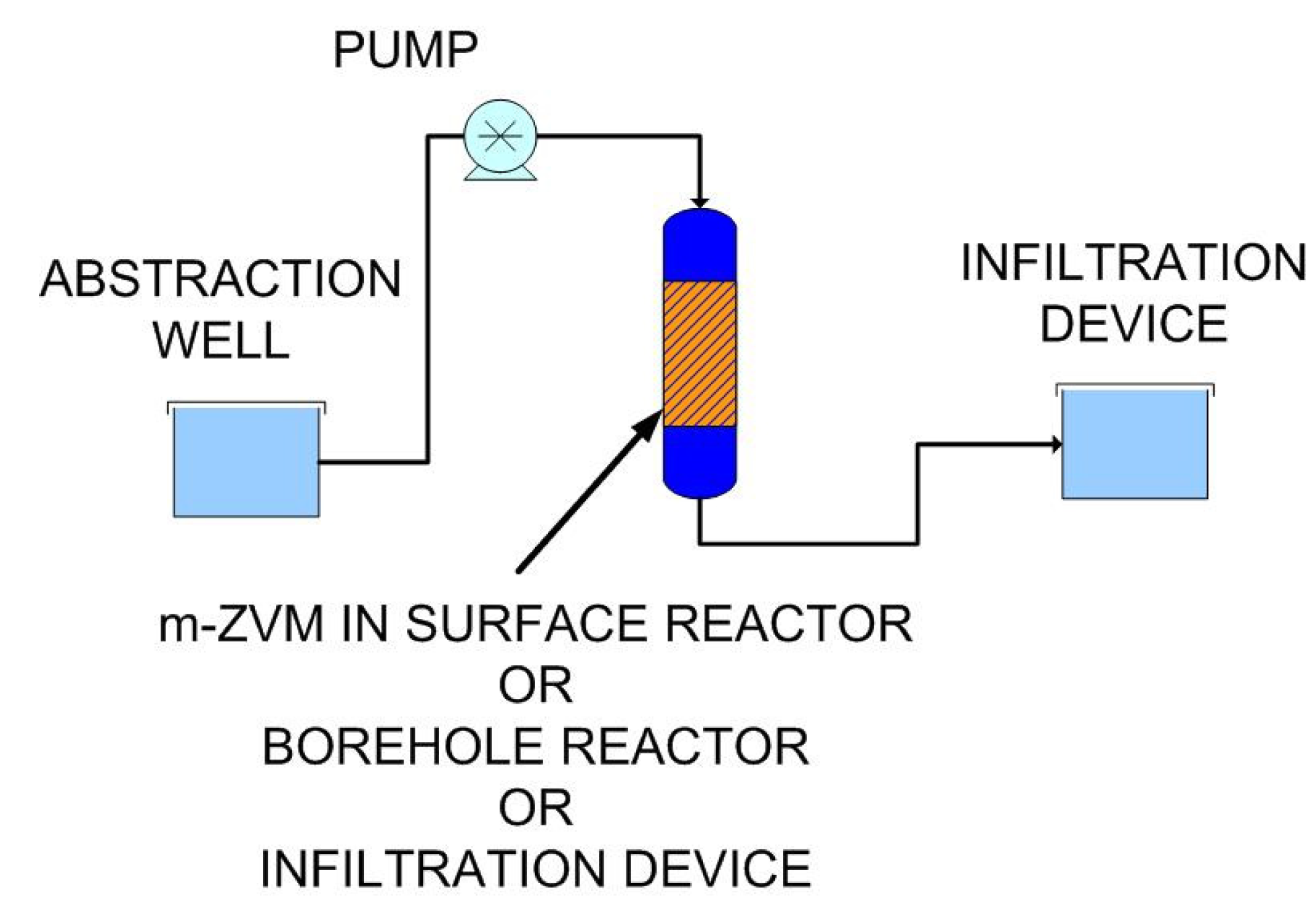
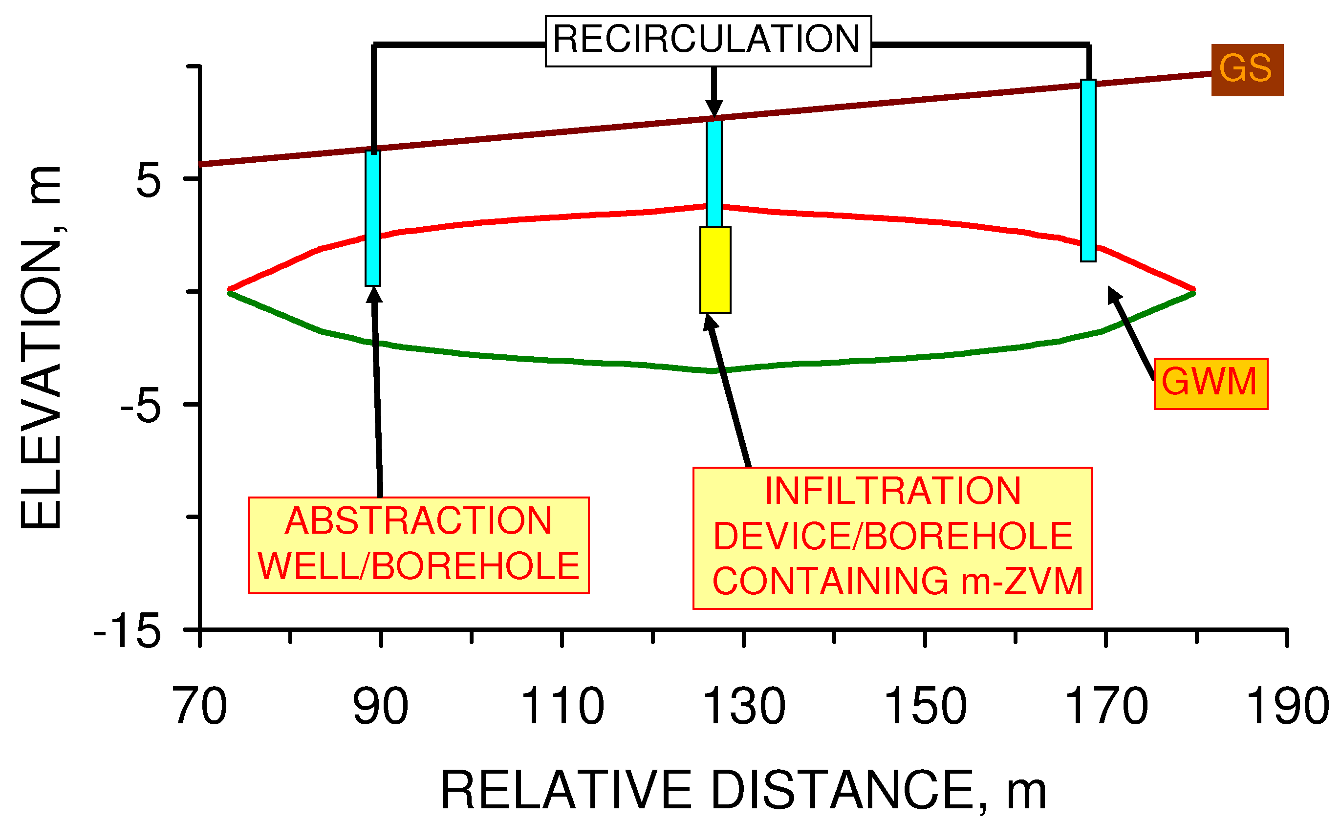
4.
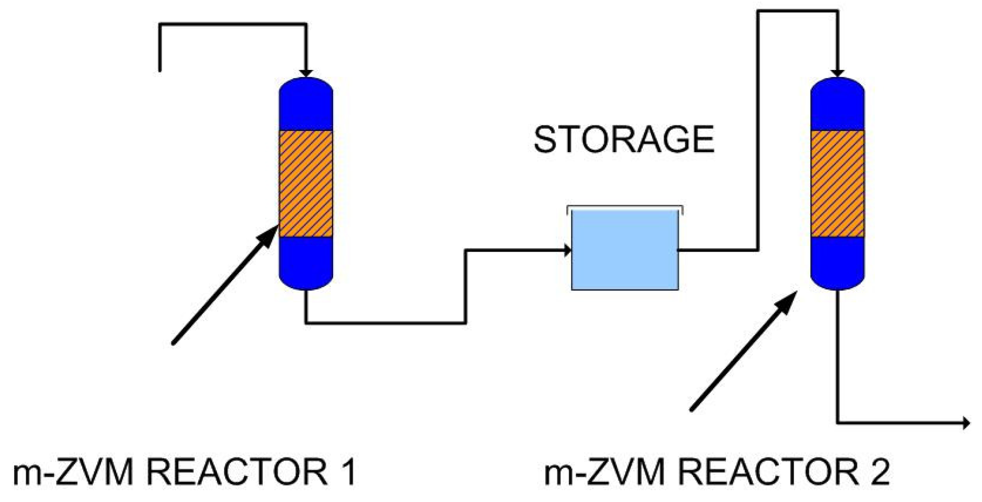
abstracting water from the aquifer, passing it through m-ZVM, and then infiltrating/injecting the treated water into the aquifer using a process of continuous recirculation.
Static diffusion tests containing clays and n-ZVM sometimes result in the n-ZVM resting on undisturbed clay layers (Figure 46a, b). The n-ZVM may contain a distinct undisturbed layer and overlying disturbed layer (Figure 46c). The disturbed layer contains O2(g) bubbles, microfractures and macropores. Some of the latter discharge at the n-ZVM water surface (Figure 46c, d). The clay layer also contains microfractures and O2(g) bubbles (Figure 46b). This observation indicates that the water contained in the n-ZVM interacts with adjacent clay layer(s). Reduction of water within the clay creates macropore conduits, which allow ion exchange to occur between the clay and the n-ZVM. For example, the substitution of Na, Ca, Mg, Al cations by Fe2+ and Fe(a−n)+H(aq) at low pH [79,80,81,82,83,84,85] and by Na+ at high pH (e.g., >8) [86].
These observations suggest that delivery of m-ZVM treated water to an aquifer containing Fe(a−n)+H(aq) may result in a proportion of the Fe(a−n)+H(aq) ions substituting cations (Mg, Ca, Mn, Sr, K, Na, Al, etc.) within clays contained within the aquifer. This pillaring process will create catalytic sites within the clay nano-environment, which can both crack/reduce organic chemicals (pollutants) and polymerise COx, CxHy, CxHyOz, CxHyClz into hydrocarbons and other compounds [85].
Figure 42. m-ZVM: Fe Ion formation vs. Change in Eh. (a) BR1, (b) BR2, (c) BR3. Fe ion concentration, mg L−1 = c [EC:ECInitial − 1]. c is approximated as 0.5. c approximates to 0.55 for water dominated by NaCl and 0.75 for water dominated by calcium bicarbonate [72].
Sustainability 02 02988 g042
Figure 43. m-ZVM: Fe Ion formation vs. Change in pH. (a) BR1, (b) BR2, (c) BR3.
Sustainability 02 02988 g043
Figure 44. n-ZVM: Fe Ion formation vs. Change in Eh. (a) DR1, (b) DR2, (c) DR3.
Sustainability 02 02988 g044
Figure 45. n-ZVM: Fe Ion formation vs. Change in pH. (a) DR1, (b) DR2, (c) DR3.
Sustainability 02 02988 g045

4.1.3. Implications of Aquifer Equilibrium Redox Oscillations on Fe Ion Type

All aquifers are in a perpetual state of redox disequilibrium [6,7], though the variation in redox parameters and associated oscillation may decrease with time and SV. The relationship between ion formation and ion type was assessed (Figure 47 and Figure 48) for each oscillation where there is an increase in ion concentration for m-Fe0 (MWR1) and m-Fe0 + m-Al0 + m-Cu0 (MWR5). The equilibrium oscillation results in shifts between FeOH+ and Fe(a−n)+Hn formation (Figure 47 and Figure 48). The relationship between ion type and SV (Figure 49) indicates that at high SV the dominant ion type is Fe(a−n)+Hn. However, at lower SV there is an oscillation between FeOH+ and Fe(a−n)+Hn formation (Figure 49).

4.1.4. Implications for Clays within the Aquifer

Smectites, including montmorillonite (Figure 46), have a 2:1 dioctahedral structure where a sheet of octahedrally coordinated metal cations is sandwiched between two tetrahedral (Si) layers [87]. Substitution of the octahedral cations by a bivalent (e.g., Fe), or monovalent (e.g., Na) metal ion creates a net negative inter-layer charge. This creates an interaction with exchangeable cations to form both a hydrated phase and a catalytic surface. These cations and surfaces react strongly with polar substances, which migrate into the inter-layer spaces.
The static diffusion tests (using n-ZVM) have demonstrated that in an aggressive H2O reduction saline environment the clay mixes and becomes intermingled with the n-ZVM (Figure 41a) while in more benign saline (Figure 6) and freshwater (Figure 46) reducing environments the clay remains distinct from the n-ZVM. However, even in the more benign environments there is an interaction between the clays and the n-ZVM which results in the formation of extensive macropore conduits (Figure 5 and Figure 46), fractures (Figure 46) and O2 discharge (Figure 5, Figure 6 and Figure 46). These conduits allow free passage of water between the aquifer, n-ZVM bed and the clay (e.g., Figure 46). This allows substitution of inter-layer cations by Fe(a−n)+Hn, Fe2+ and other cations contained within the water (e.g., Cu, Mg, Mn, Sr, K, Na, etc.). Substitution results in the development of an equilibrium interaction between hydration, or absorption, potential of the inter-layer cations, Eh, pH, charge site density, surface area, and type of adsorbed cation. The hydration, or absorption, potential varies as a function of pH and the absorption-desorption coefficient, P/Po [86].
Figure 46. Cross sections through n-ZVM beds where the clay remains as a distinct layer overlain by n-ZVM. Figure 46a,b,d show the n-ZVM-water contact. (a) Vuggy, fractured disturbed n-ZVM layer (containing O2 bubbles) overlying clay. Field of view 20 mm. (b) Vuggy, fractured disturbed n-ZVM layer (containing O2 bubbles) overlying clay. The clay contains fractures and O2 bubbles. Field of view 20 mm. (c) Vuggy, fractured disturbed n-ZVM layer (containing O2 bubbles) overlying undisturbed n-ZVM layer. Field of view 10 mm. (d) Enlargement of air-n-ZVM interface in Figure 46a demonstrating that the fracture networks within the n-ZVM discharge into the overlying water; 12 days after bed formation: Eh = −0.358 V; pH = 9.25; EC = 0.701 mS cm−1; T = 17.8 °C. Freshwater charge: Eh = 0.164 V; pH = 6.42; EC = 0.253 mS cm−1: n-ZVM bed weight ratio: 7.7 Ca-montmorillonite: 6.5 n-Fe0: 1.67 n-Al0: 1 n-Cu0.
Sustainability 02 02988 g046
Adjustment of the aquifer pH and Eh by either static diffusion or recirculation through m-ZVM will alter the equilibrium concentration of cations in the inter-layer space and will alter the cation hydration levels [87] and water composition by changing clay adsorption capacities for specific ions. This allows aquifers, which contain smectites to be actively managed to remove, breakdown, and where appropriate store specific cations from the water (e.g., Na (in saline water), various metals ions, organic compounds, gases (e.g., CH4, CO2)). Addition of specific cations to the aquifer water will allow cation substitution to be targeted to catalytically remove specific pollutants from the water.
Figure 47. m-ZVM: Fe Ion formation vs. Change in Eh. (a) MWR1, (b) MWR5.
Sustainability 02 02988 g047
Figure 48. m-ZVM: Fe Ion formation vs. Change in pH. (a) MWR1, (b) MWR5.
Sustainability 02 02988 g048
Figure 49. m-ZVM: Fe Ion formation vs. SV. (a) MWR1, (b) MWR5.
Sustainability 02 02988 g049

4.2. Applicability of Regression Equations to the Modeling of Pore Water Redox Modification

A n-ZVM injection program will result in an aquifer permeability reduction and an associated subsequent modification of the pore-water by static diffusion. This study has identified two alternative remediation strategies, which will allow remediation without reducing the permeability of the aquifer. They are:
  • static diffusion associated with placement of the m-ZVM in an infiltration/observation well (e.g., Figure 50).
  • Recirculation associated with placement of the m-ZVM in an infiltration/injection device/borehole with continual abstraction and reinjection/reinfiltration of the water (e.g., Figure 51).
These process flows (Figure 50 and Figure 51) can be applied to any aquifer containing a plume (or body) of contaminated water. These two strategies allow modeling of the expected changes in redox environment in a contaminated groundwater plume. The specific advantage of targeting remediation in a self-sealing GWM is that the perched high permeability GWM is in a clayey sequence. This allows the creation of water-clay interfaces (Figure 6 and Figure 46) where fracture networks associated with H2O reduction (to O2) extend the storage capacity of the GWM (Figure 5) and allow the water within the GWM direct access to the inter-layer spaces within the clay (Figure 46). This allows the direct cation substitution with Fe and the creation of highly polar nano-sites within the inter-layer spaces, thereby increasing the removal of organic compounds, chlorinated compounds, and metals.
Figure 50. Example Self-Sealing Groundwater Mound (GWM) fed by an infiltration device containing m-ZVM. GS = Ground surface. GWM upper surface denoted in red. The GWM lower surface is denoted in green. The recharge and permeability parameters defining the GWM are provided in [1].
Sustainability 02 02988 g050

4.2.1. Reference Pilot n-ZVM Pilot Injection Program

The published results of a n-ZVM program at Naval Air Station (NAS) Jacksonville, Florida, USA [6] were used to assess the applicability of the experimental regression relationships to n-ZVM and m-ZVM treatment programs using both static diffusion and continuous recirculation.
The n-ZVM pilot program utilized abstraction and injection wells [6]. During an initial period of 23 h water was continuously abstracted and reinfiltrated through the contaminated aquifer [6]. The reinfiltrated water contained 2–4.5 g L−1 n-Fe0 (with 0.1% palladium, 50–300 nm particle size) [6]. Infiltration was into an unconfined sand/silt aquifer (2.1–7.3 m bgs) [6]. About 11.34 kg n-Fe0 was infiltrated through 6 infiltration wells (total of 2.8–5.6 m3 H2O infiltrated) [6]. The infiltration in specific wells ceased after about 17 h due to pore blockage [6]. The estimated contaminated aquifer gross rock volume = 220 m3–698 m3; estimated contaminated net pore-water volume = 108 m3−350 m3. Pre-treatment volatile organic compounds, VOC’s, were <83 mg L−1 (including <26 mg L−1 tri-chloro-ethenes (TCE), 1.3 mg L−1 di-chloro-ethenes (DCE)) [6]. The aquifer pore-waters were modified by static diffusion by the infiltrated n-ZVM within the aquifer pore space.
Post infiltration, pore-water monitoring [6] indicated a 65−99% reduction in parent VOC’s during a 5 week period. This was associated with an increase in Fe ions (from 3.5 mg L−1 to 15 mg L−1), increase in pH (of 0.07–0.49), and a decrease in Eh (ORP) (of 0.250–0.368 V). pH and Eh at the onset were 5.77 to 5.96 and −0.034 to +0.1114 V respectively. The 5 week SV = 10.9 for 108 m3 pore-water and 35.3 for 350 m3 pore-water.
This study uses the NAS Jacksonville aquifer pilot study starting pH and Eh [6] as a reference for modeling. The experimental regression relationships are used to determine if modeling based on m-ZVM (static diffusion) or n-ZVM (continuous recirculation) or m-ZVM (continuous recirculation) are able to replicate the NAS Jacksonville aquifer Eh, pH environment after a 5 week period [6].
Figure 51. Example Self-Sealing Groundwater Mound (GWM) fed by an infiltration device/borehole containing m-ZVM, where water is continually abstracted and reinjected/reinfiltrated into the GWM. GS = Ground surface. The recharge and permeability parameters defining the GWM are provided in [1].
Sustainability 02 02988 g051

4.2.2. Modeling Static Diffusion: m-ZVM

In the process configuration illustrated in Figure 50, effective SV decreases with increasing distance from the infiltration device, ID. Vw (Equation 8) defines the average SV within a specific perimeter boundary. Average SV decreases with increasing time and increasing radius around the ID. This allows Eh, pH and EC to be estimated as a function of time and distance from the ID, during the design phase for a remediation program using the regression Equations 12 to 26 for specific m-ZVM combinations.
The expected changes in redox parameters are:
Change in Eh = Regression EhEhInitial
Change in pH = Regression pHpHInitial
Change in EC = (Regression EC:ECInitial Ratio – 1) × ECInitial
The expected change in average redox parameters for 11.34 kg m-ZVM placed in an infiltration device/well/borehole (Figure 50) and pore water volume contained in the GWM after 5 weeks is summarised in Figure 52 as a function of water volume within the GWM for m-Fe0 (MWR1) and m-Fe0 + m-Cu0 + m-Al0 (MWR5). This analysis (when compared with the n-Fe0 + Pd0 NAS Jacksonville observations [6]) indicates that m-Fe0 + m-Cu0 + m-Al0 will produce a similar average Eh change to n-Fe0+Pd0 (Figure 52a). MWR1 and MWR5 produce a greater average increase in pH than Fe0 + Pd0 (Figure 52b).
Figure 52. Modeled static diffusion change in average Eh and pH as a function of water volume after 5 weeks. (a) Eh Change (b) Average pH Change, 11.34 kg m-ZVM. NAS Jacksonville data from [6].
Sustainability 02 02988 g052

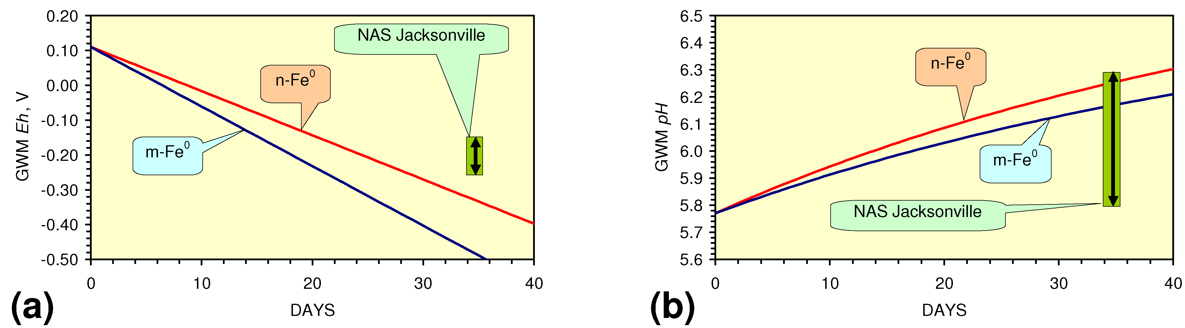
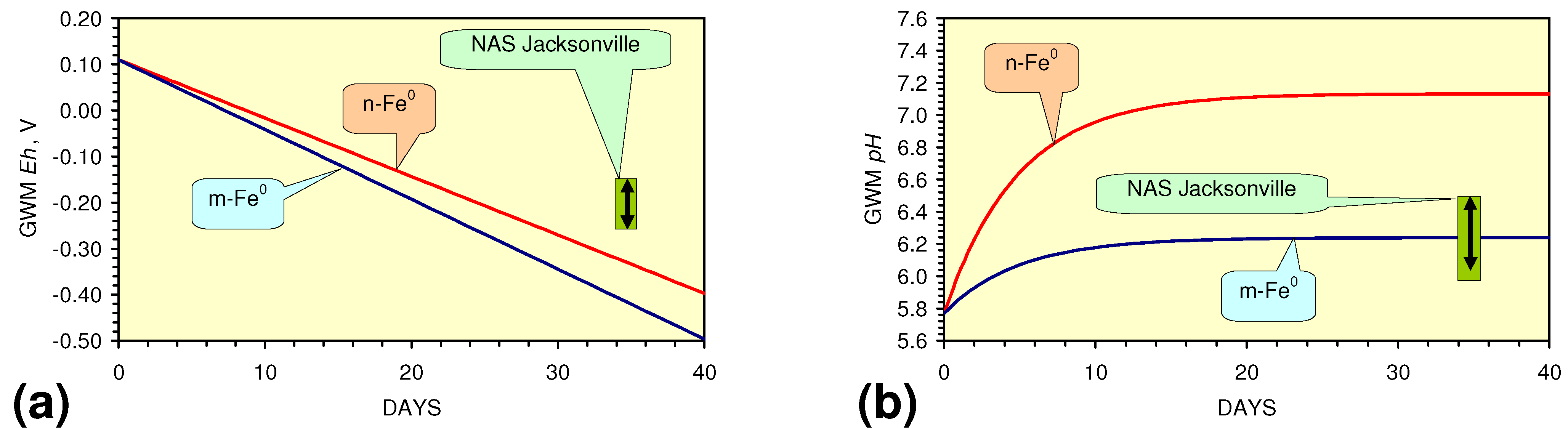
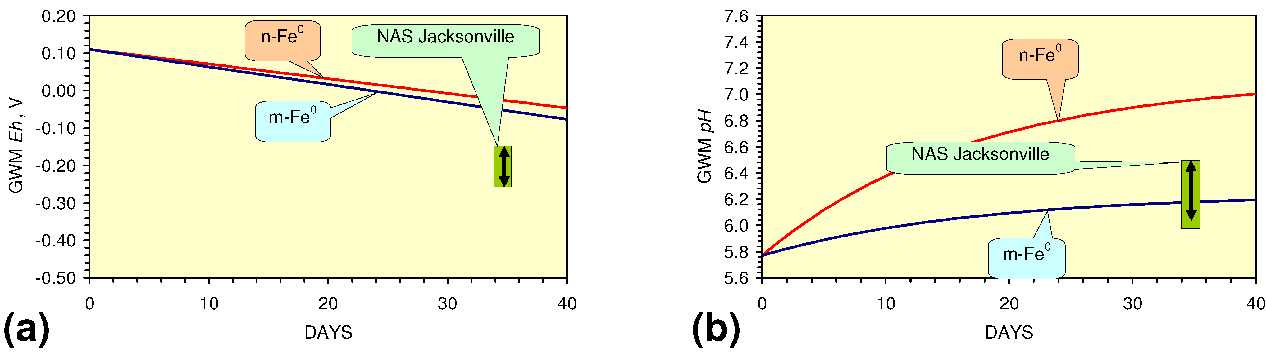
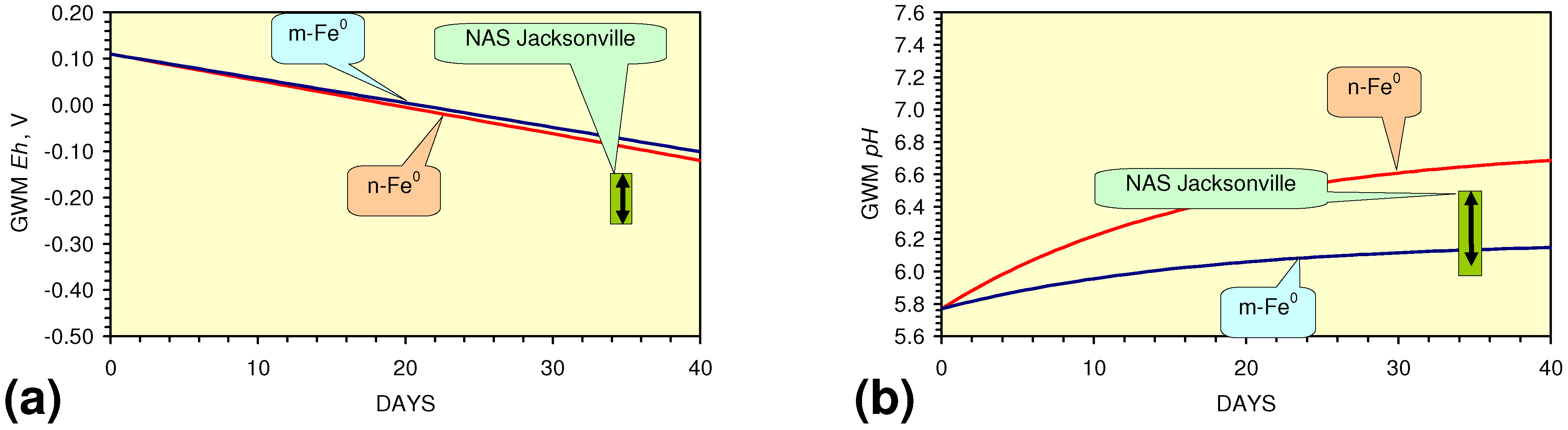
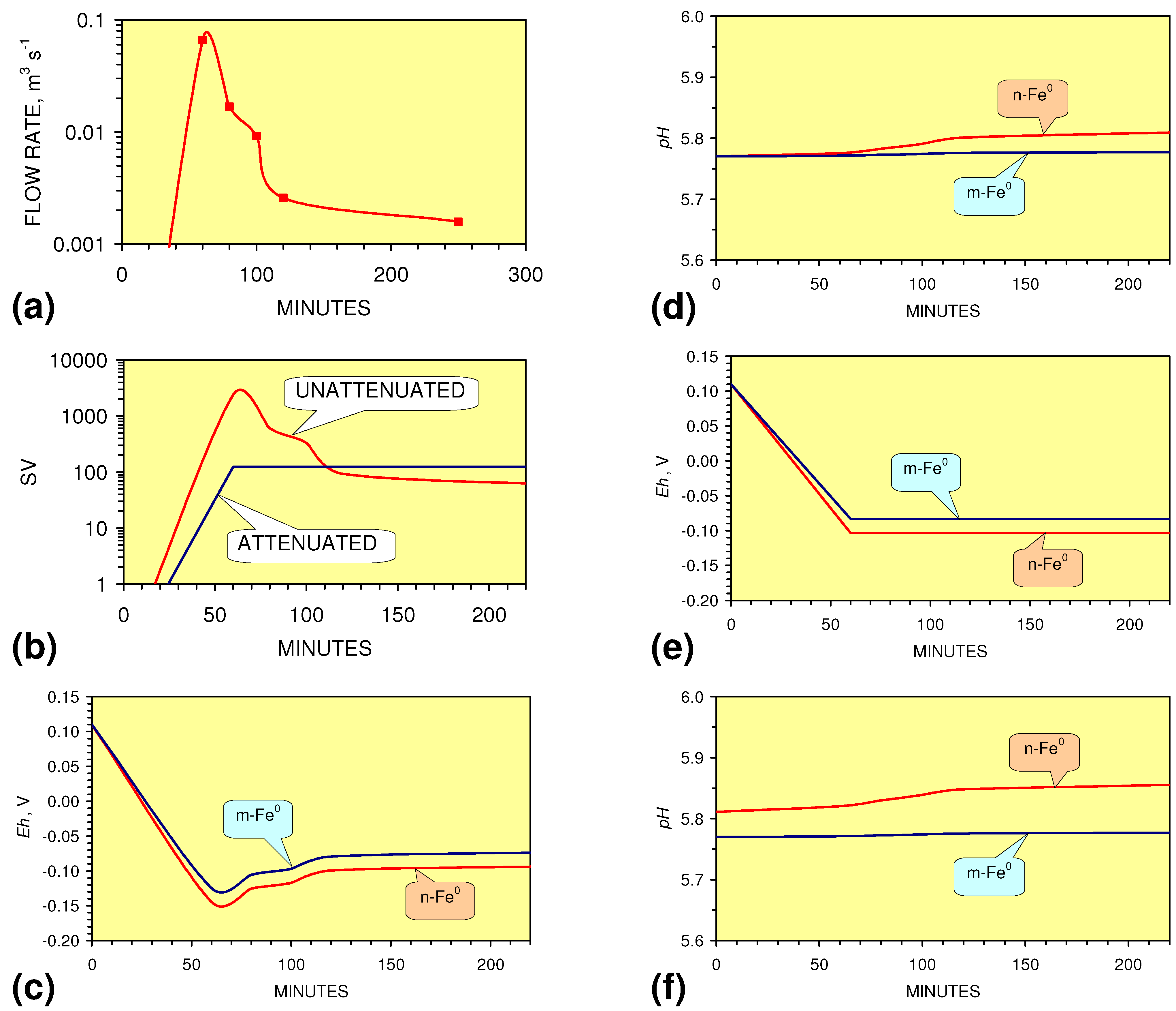
4.2.3. Modeling Redox Modification by Recirculation: m-ZVM

The process configuration illustrated in Figure 51 requires a continual water circulation through a reaction zone containing m-ZVM (Figure 53). The change in redox parameters can be modelled using the regression Equations 27–35 for n-ZVM and 36–53 for m-ZVM.
Eh (time = n + 1 days) = (1 − a) Eh(time = n days) + a (Eh(time = n days) + [Regression Eh-EhInitial + Eh(time = 0 days)])
pH (time = n + 1 days) = (1 − a) pH(time = n days) + a (pH(time = n days) + [Regression pH pHInitial + pH(time = 0 days)])
EC:ECInitial(time = n + 1 days) = (1 − a) EC:ECInitial (time = n days) + a [Regression EC:ECInitial]
Fe ion concentration (time = n + 1 days) mg L−1 = c [EC:ECInitial (time = n + 1 days) − 1]
a = proportion of aquifer volume recirculated each day; c = relationship between EC and Fe ion concentration. EhInitial and pHInitial refer to the average Eh and pH in the feed water associated with the regression Equations 27–35 and 36–53.
The Jacksonville GWM/contaminated plume contained 108 m3 water (pH = 5.77; Eh = 0.103 V). Modelling a recirculation (abstraction and infiltration) rate of 0.83 m3 h−1, operated with an SV of 100 (i.e., 8.3 kg n/m-ZVM) will gradually change the Eh and pH of the entire GWM/plume.
  • The continuous flow tests indicate that utilisation of m-Fe0 would require replacement of the m-Fe0 after about 20 m3 of water had been processed.
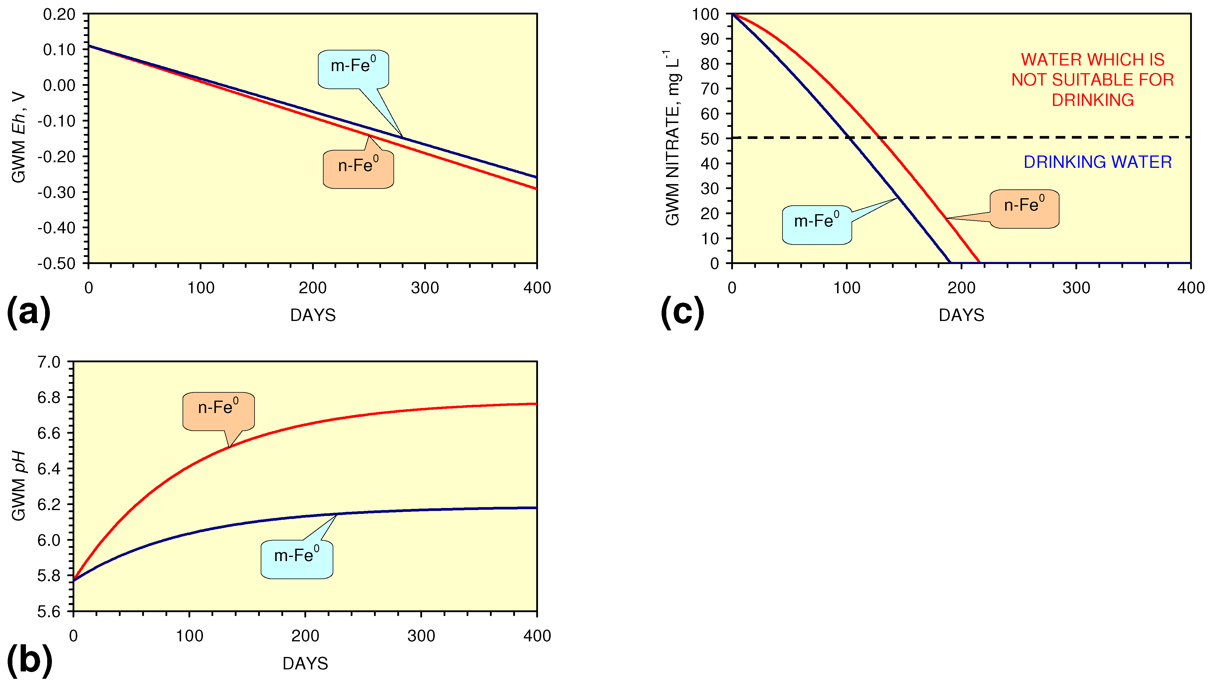
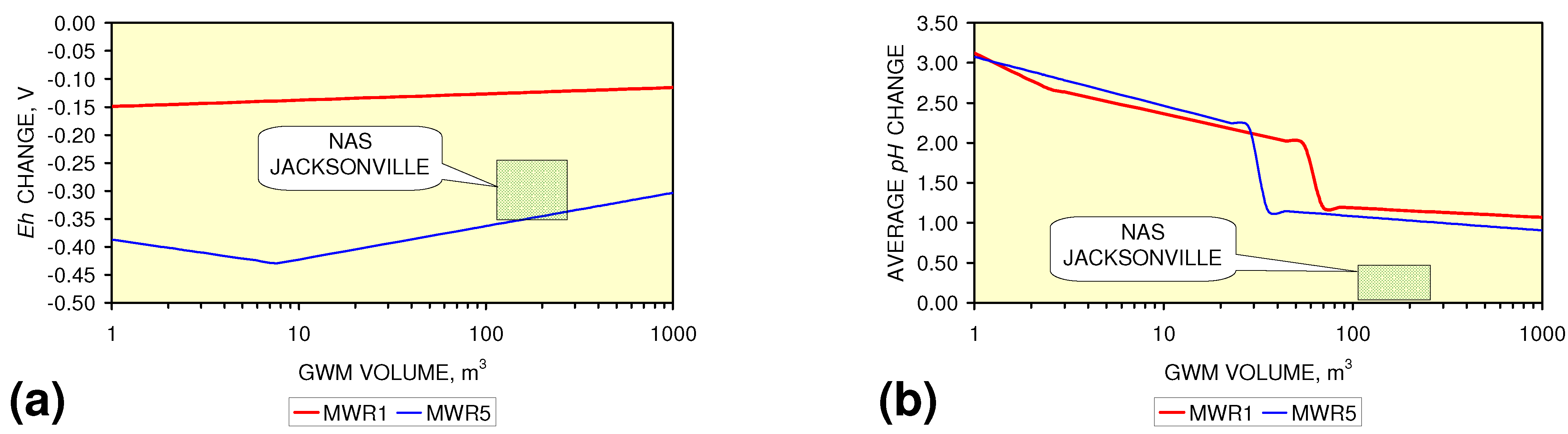
  • m-Fe0 will provide a lower Eh in the GWM after 40 days than n-Fe0 (Figure 54)
  • m-Fe0 will provide a lower pH in the GWM after 40 days than n-Fe0 (Figure 54)
  • the modelling provides a similar Eh and pH to the NAS Jacksonville pilot tests [6] (Figure 54), indicating that recirculation through m-Fe0 may form an effective remediation approach.
  • Reducing the SV to 10, while maintaining a circulation rate of 0.83 m3 h−1 (i.e., using 83 kg n/m-ZVM), has the effect of establishing an equilibrium pH in the aquifer while reducing the decrease in Eh (Figure 55).
In many remediation environments, the actual volume of the contaminated groundwater is unknown. For example undertaking a remediation strategy utilising an SV of 10 (Figure 55), without increasing the recirculation rate, where the effective aquifer volume is actually 350 m3 has the effect of reducing the expected changes in Eh and pH (Figure 56). In this instance reducing the amount of ZVM in the recirculation circuit (Figure 53) (or increasing the pump/recirculation rate) will increase the effective SV and offset, or partially offset, the adverse effects on Eh (Figure 57) resulting from the aquifer volume being larger than predicted.
Figure 53. Process flow between the abstraction well and infiltration device, when redox modification results from a continual water circulation.
Sustainability 02 02988 g053
Figure 54. Modeled recirculation change in average Eh and pH as a function of water volume after 5 weeks. (a) Eh Change, (b) Average pH. SV = 100; GWM/plume contains 108 m3; Recirculation rate = 20 m3 d−1; 8.3 kg n-Fe0. NAS Jacksonville data from [6].
Sustainability 02 02988 g054
Figure 55. Modeled recirculation change in average Eh and pH as a function of water volume after 5 weeks. (a) Eh Change, (b) Average pH. SV = 10; GWM/plume contains 108 m3; Recirculation rate = 20 m3 d−1. 83 kg n-Fe0. NAS Jacksonville data from [6].
Sustainability 02 02988 g055
Figure 56. Modeled recirculation change in average Eh and pH as a function of water volume after 5 weeks. (a) Eh Change, (b) Average pH. SV = 10; GWM/plume contains 350 m3; Recirculation rate = 20 m3 d−1. 83 kg n-Fe0. NAS Jacksonville data from [6].
Sustainability 02 02988 g056
Figure 57. Modeled recirculation change in average Eh and pH as a function of water volume after 5 weeks. (a) Eh Change, (b) Average pH . SV = 100; GWM/plume contains 350 m3; Recirculation rate = 20 m3 d−1. 8.3 kg n-Fe0. NAS Jacksonville data from [6].
Sustainability 02 02988 g057

4.3. Potential Applications

The test regression modeling (Figure 54, Figure 55, Figure 56 and Figure 57) indicates that m-ZVM modeling can be used to predict the behavior of a remediation project during the design phase. This allows:
5.
Remediation of storm runoff water/overland flow volumes to be predicted from specific design storms [88,89,90] or specific storm runoff hydrographs [1,89,90]
6.
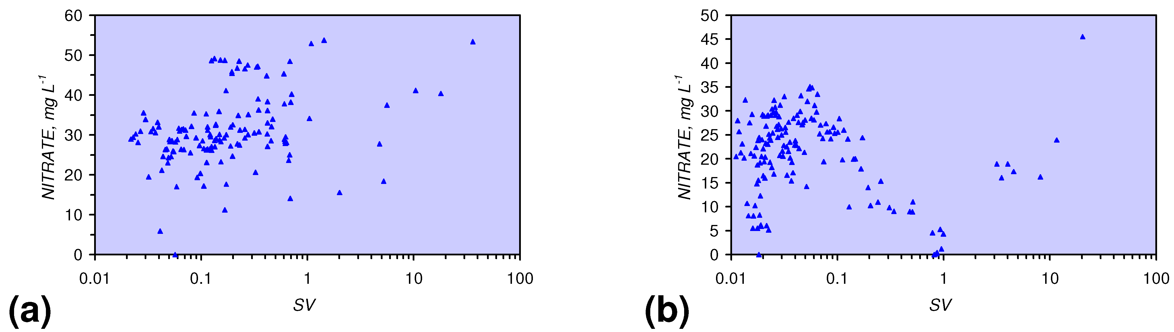
Remediation of specific anions (e.g., nitrates) to be predicted for static diffusion PRB’s and recirculation remediation programs
7.
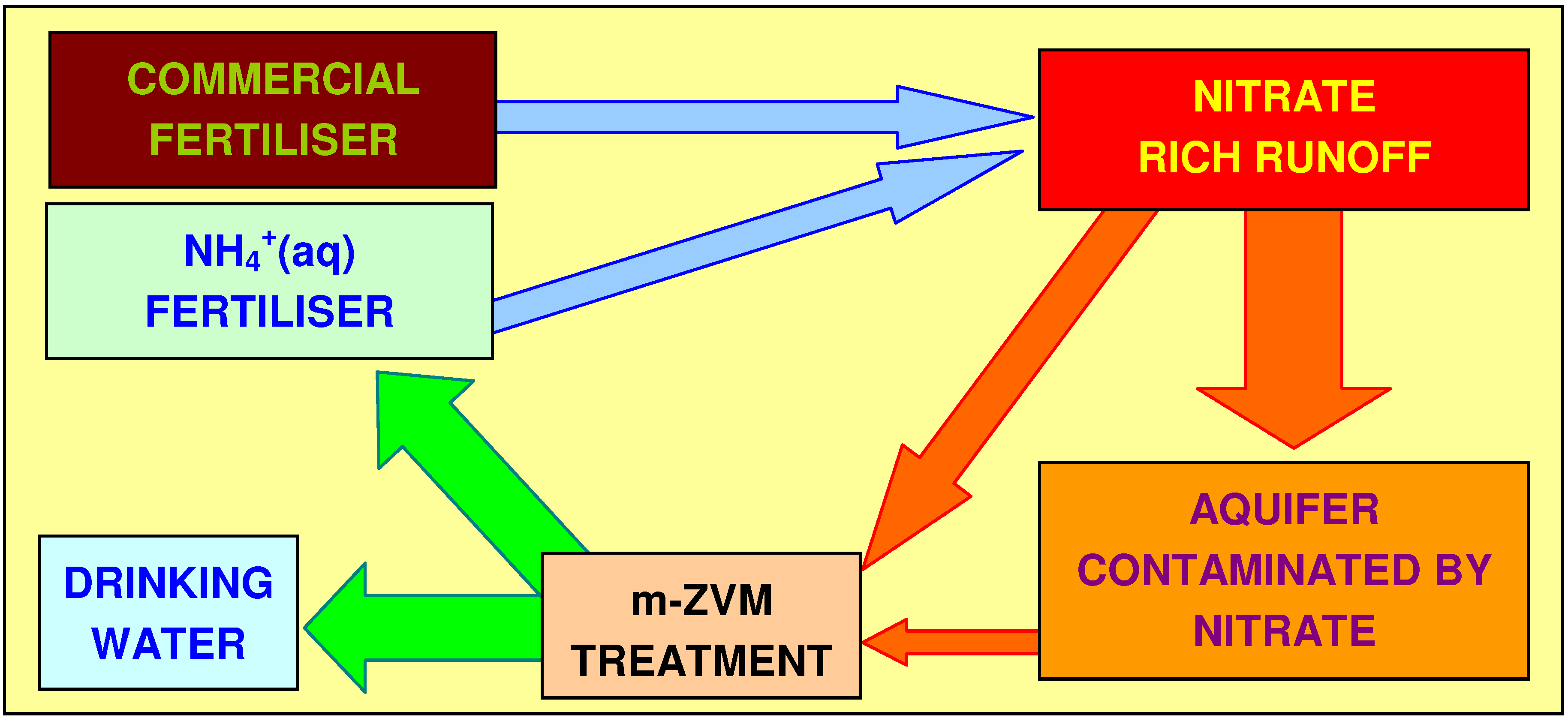
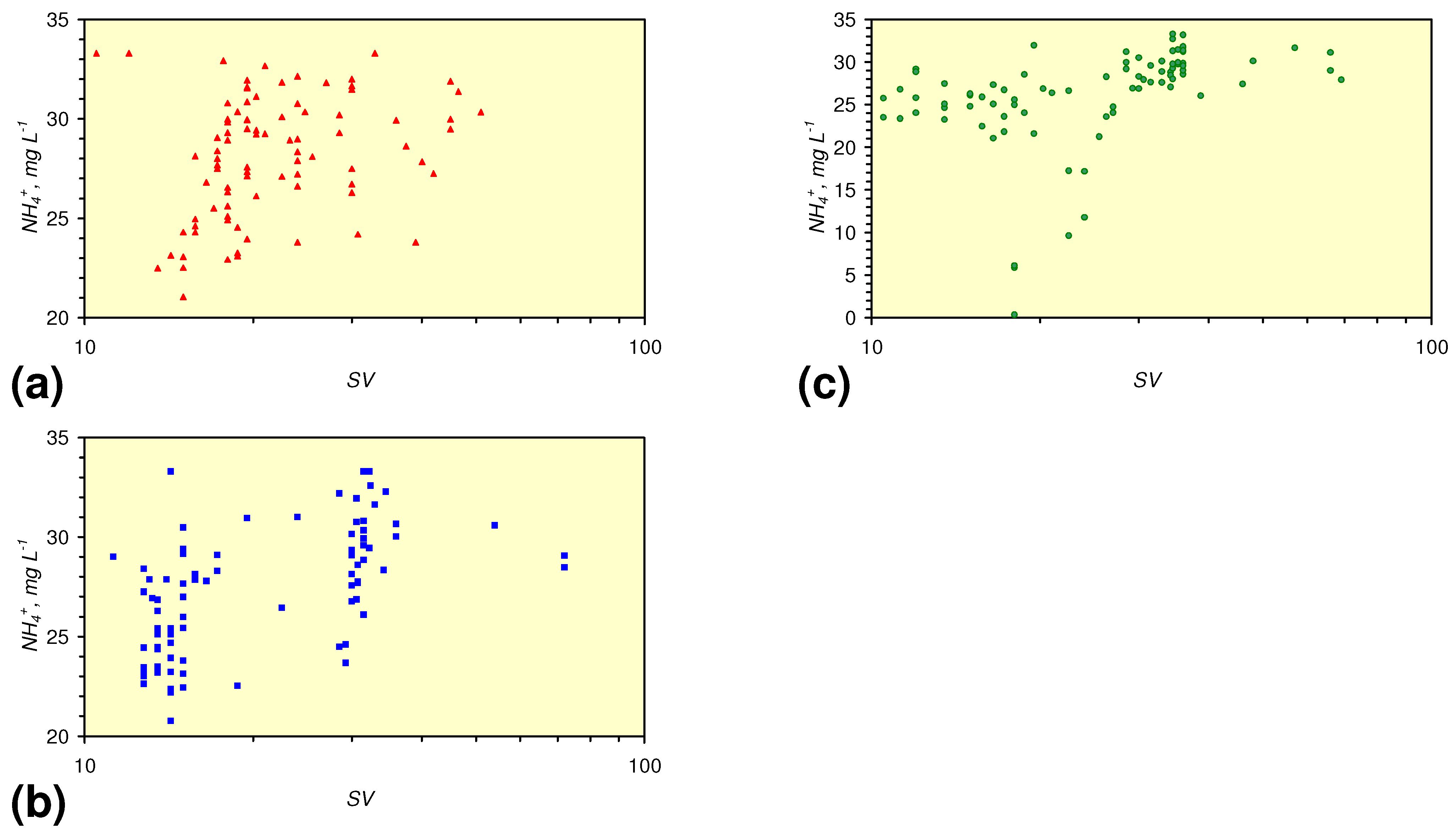
Enrichment of specific cations (e.g., ammonia) to be predicted for static diffusion PRB’s and recirculation remediation programs which are designed to convert nitrate enriched groundwater into nitrogen enriched agricultural fertiliser
8.
Remediation of specific cations (e.g., Cu, Pb) to be predicted for static diffusion PRB’s and recirculation remediation programs
9.
Remediation of organic contaminants to be predicted for static diffusion PRB’s and recirculation remediation programs
10.
Aquifer remediation programs to be designed based on recirculation
Pre-construction modeling during the design for remediation projects allows the actual observed post-construction remediation levels to be compared with the pre-construction forecast.

4.3.1. Remediation of Storm Runoff/Overland Flow

Infiltration devices receiving storm runoff or overland flow discharge (Figure 50) the water into a GWM or aquifer [1,2,88,91,92,93]. The infiltration devices are designed to remove suspended solids prior to infiltration [88,91,92,93]. The storm runoff water may be contaminated by nitrates (e.g., agricultural runoff), hydrocarbons/organic chemicals (road runoff/chemical runoff), salt (road runoff/irrigation project runoff) and metals (e.g., road runoff/industrial runoff/mining runoff) [92,94]. The infiltrating water will either flow directly into the water table [89,90], or into the water table via a descending groundwater mound [1,95], or into the water table by lateral propagation of a perched groundwater mound [96], or will form a perched sealed groundwater mound [1,2]. Surface runoff will form a perched water table confined to the upper layers of the topsoil [8,97], which may also intersect and enter the infiltration device. Adjoining groundwater mounds associated with different infiltration devices may intersect each other in the subsurface [1,2,97]. Placement of submerged m-ZVM in the infiltration device (Figure 50 and Figure 53) or in a flow line feeding the infiltration device (Figure 58 and Figure 59) will allow the feed water to be treated by
  • adjusting the equilibrium ion concentrations, and
  • placing Fe(a−n)+H ions (i.e., Fe catalyst) in the infiltrating water.
For example, a typical storm runoff hydrograph [1] from a large catchment area (Figure 60a) has a high peak flow followed by a period of reduced flow. This results in very high SV’s if the runoff water is treated in a flow line without attenuation (Figure 60b) and a variable Eh and pH in the treated water (Figure 60c, d). Attenuation in a storage unit (e.g., detention basin, retention basin, pond [91,92,93]) prior to treatment and infiltration (Figure 59) means the SV can be reduced to a constant level (Figure 60b). This results in a constant redox in the treated water entering the infiltration device (Figure 60e, f). This analysis demonstrates that m-ZVM can be used to treat storm runoff water prior to (and during) infiltration into an aquifer.
Figure 58. m-ZVM reactor used to treat water prior to discharge into an infiltration device.
Sustainability 02 02988 g058
Figure 59. m-ZVM reactor used to treat attenuated water prior to discharge into an infiltration device.
Sustainability 02 02988 g059
Figure 60. Analysis of Storm Runoff Treatment. (a) Storm runoff hydrograph (Total runoff = 297 m3). (b) SV as a function of flow rate for 100 kg Fe0. Attenuated flows are based on an average flow from the attenuation device of 29.7 m3 h−1. (c) Expected Eh for unattenuated flow. (d) Expected pH for unattenuated flow. (e) Expected Eh for attenuated flow. (f) Expected pH for attenuated flow. Runoff Eh = 0.11 V, pH = 5.77.
Sustainability 02 02988 g060

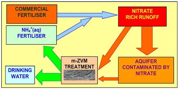
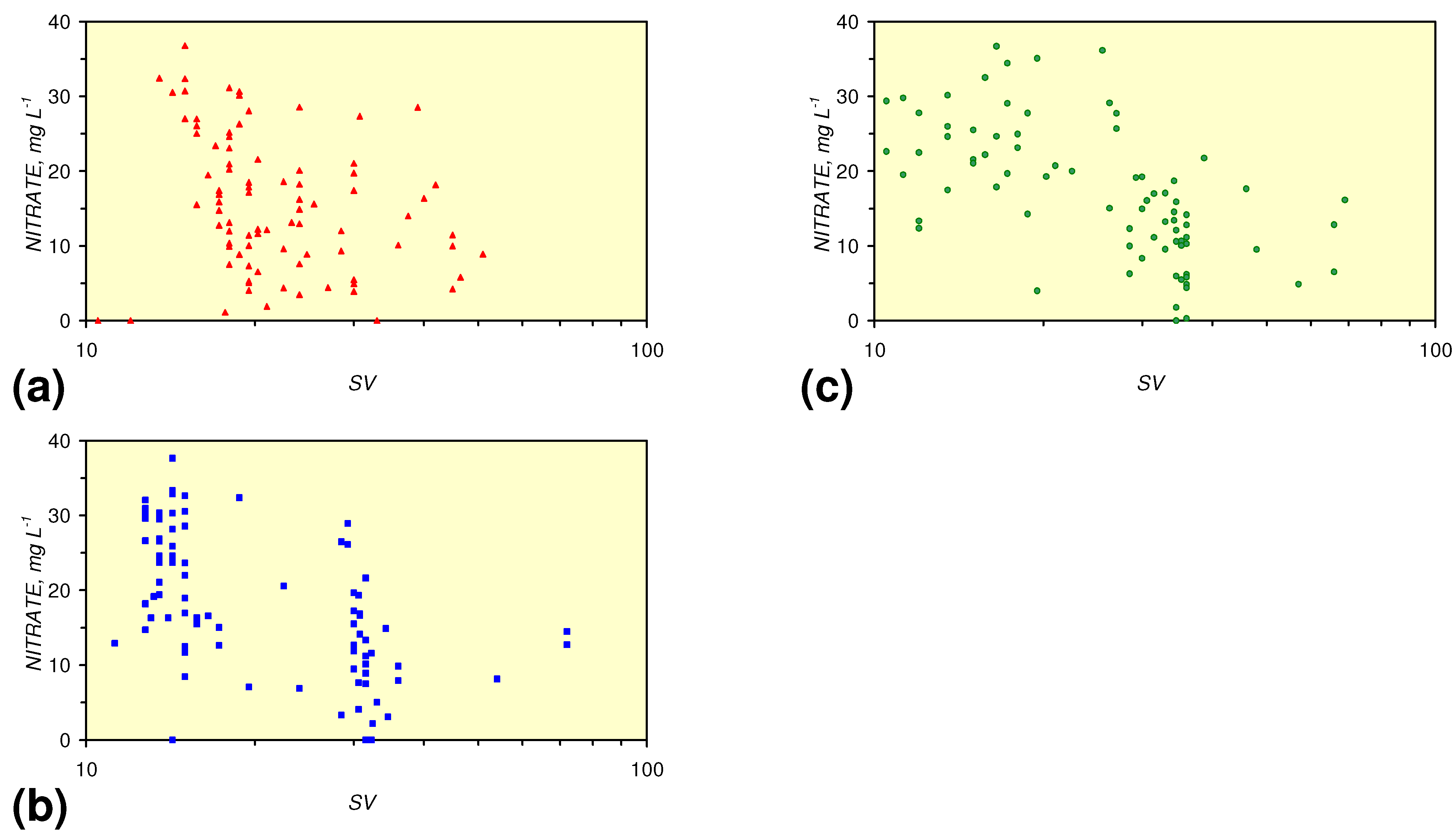
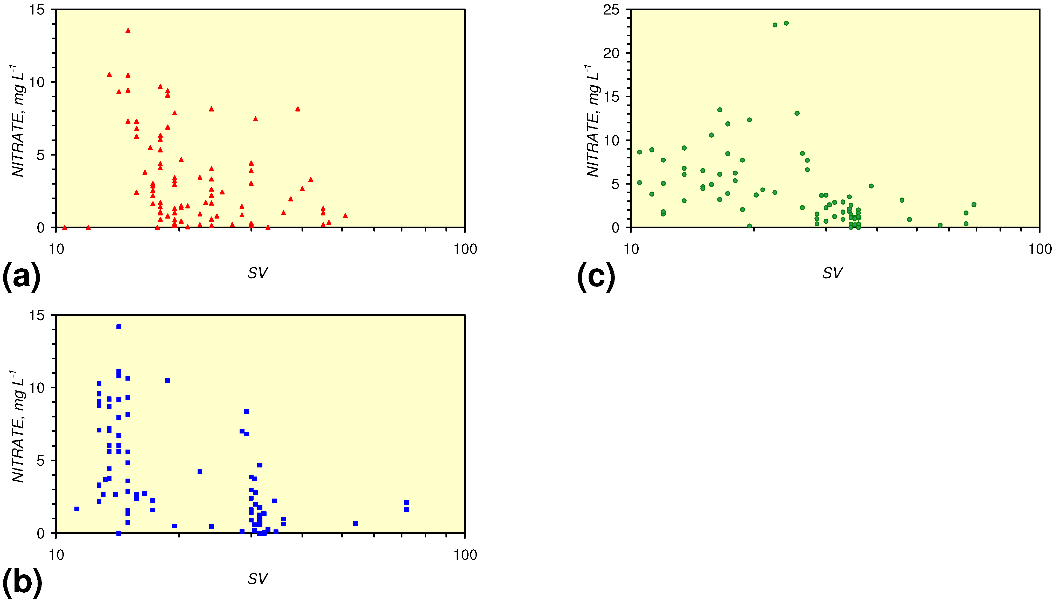
4.3.2. Nitrate Remediation

The redox environment defines the ion type [73] and relative concentration [35,36,37,73]. The redox fences can be viewed as equilibrium concentration boundaries [73]. For example, the equilibrium concentrations of NH4+ and NO3at the NH4+: NOxredox boundary are [1 − a]:[0 + b] (Eh3) (Figure 61). Similarly the equilibrium concentrations of NH4+ and NO3 at the NH4+: NO3 redox boundary are [0 + a]:[1 − b] (Eh2) (Figure 61). a and b vary with Eh for a specific boundary and reflect the reaction quotient (Equation 2). They are very small [35,36,37]. For design modeling purposes a = 0 and b = 0.
Since the redox boundaries are known [73] (Figure 61), it follows [35,36,37] that the equilibrium NO3 concentration (I1) can be estimated for a specific Eh and pH and specific NO3concentration in the feed water (I2) as (Equilibrium or Low SV Case):
I1 (mg L−1) = I2 (Eh Eh3)/(Eh2 Eh3) c
c = correction factor (e.g., 1.0) which may vary with Eh, pH, temperature, SV, and water composition. In the continuous flow reactors (and SDR’s with high SV (Figure 61) the Eh of the feed water (Eh1) defines the ion concentration, I1 (High SV Case):
I1 (mg L−1) = I2 (Eh Eh3)/(Eh1 Eh3) c

4.3.2.1. PRB Nitrate Remediation

GWM/aquifer remediation using n-ZVM placed in PRB’s (SDR’s) will remove nitrates [40]. Batch experiments demonstrated experimentally that m-Fe0 will remove nitrates [41] by static diffusion. Figure 61 illustrates (for an SDR, PRB) the initial change in Eh:pH where the nitrate concentration is controlled by Equation 76, and the oscillating equilibrium state where the nitrate concentration is controlled by Equation 75. The associated impact on nitrate concentrations of changing SV (Figure 62) demonstrates that nitrate concentrations initially decrease rapidly with SV (as the Eh reduces). They subsequently rise as water composition adjusts to a stable redox equilibrium position. The initial reduction in nitrate concentration can be >90% (Figure 62). However, the formation of a stable redox position results in a long term stable nitrate reduction of 50–85% in the GWM (Figure 62). The presence of m-Al0 and/or m-Cu0 increases the proportion of nitrate removed, when the water is in a stable equilibria.
Figure 61. Nitrate redox fences (Eh2, Eh3). Data values are for MWR5. Redox boundaries from [73].
Sustainability 02 02988 g061

4.3.2.2. Flowing Water: Nitrate Remediation

Nitrate removal rates of 65–95% (Figure 63) result from flowing water through m-ZVM in a single borehole reactor. Passing the water through two reactors arranged in series and separated by an intervening storage or attenuation (Figure 65) results in an increase in the nitrate removal rate (Figure 64). This analysis indicates that m-ZVM can be used to reduce nitrate concentrations by >85% in a continuous water flow (e.g., abstraction of nitrate contaminated water or agricultural runoff water prior to discharge into an aquifer).
Figure 62. Product water nitrate concentrations for a feed water containing 100 mg L−1 NO3 vs. SV. (a) MWR1. (b) MWR5.
Sustainability 02 02988 g062
Figure 63. Product water nitrate concentrations for a feed water containing 100 mg L−1 NO3 vs. SV. (a) BR1. (b) BR2. (c) BR3. Single Reactor.
Sustainability 02 02988 g063
Figure 64. Product water nitrate concentrations for a feed water containing 100 mg L−1 NO3 vs. SV. Two borehole reactors are placed in series. (a) BR1. (b) BR2. (c) BR3.
Sustainability 02 02988 g064
Figure 65. Process flow diagram for two m-ZVM reactors placed in series.
Sustainability 02 02988 g065

4.3.2.3. Regulatory Significance

Drinking water standards in the EU [98] require EC =< 2.5 mS cm−1; pH = 6.5–9.5; Al =< 200 μg L−1; NO3 =<50 mg NO3 L−1; NH4+ =< 200 mg NH4L−1; chloride =< 250 mgCl L−1; chloride =< 250 mg L−1; Na =< 200 mg L−1; Fe =< 200 μg L−1; Mn =< 50 μg L−1; sulphate =< 250 mg L−1; oxygen =< 5 mg O2L−1. The analyses (Figure 62, Figure 63 and Figure 64) identify that m-ZVM can (in static diffusion or continuous flow reactors) remediate water which is heavily nitrate contaminated (NO3 = 100 mg NO3 L−1) by providing a product water which has a nitrate concentration which is <50 mg NO3 L−1. This observation, potentially allows abstraction for drinking water from aquifers which are heavily polluted with nitrates, by either treating the abstracted water, or by remediation of the water within the aquifer.

4.3.2.4. Agricultural Significance

During remediation, the nitrate is converted to NH4+. This results in an increase in NH4+ content within the product water. The example nitrate reduction analyses (Figure 63 and Figure 64) are associated with increases in NH4+ concentration of 20–33 mg L1 (Figure 66 and Figure 67). The NH4+ levels are within the acceptable drinking water range (i.e., <200 mg L−1) [98]. Aqueous ammonia is an agricultural fertilizer [99,100]. m-ZVM treatment of abstracted nitrate contaminated water allows a substantial proportion of the nitrate to be recycled to produce dilute aqueous ammonia fertilizer which can be used in irrigation.
Figure 66. Product water NH4+ concentrations for a feed water containing 100 mg L−1 NO3 (and 0 mg L−1 NH4+) vs. SV. (a) BR1. (b) BR2. (c) BR3. Single Reactor.
Sustainability 02 02988 g066

4.3.2.5. Sustainable Nitrate Cycle

m-ZVM treatment of abstracted or In Situ nitrate polluted groundwater allows a sustainable cycle to be developed (Figure 68) where nitrate polluted surface runoff is treated during infiltration, or within the aquifer, or during abstraction, by m-ZVM to remove nitrates. The ammonia and nitrate levels of the treated water meet drinking water standards [98]. However, the conversion of nitrate to aqueous ammonia allows the N to be recycled for agricultural use as an N fertilizer during irrigation. This allows m-ZVM to be widely applied in irrigation areas to produce N enriched water which can supplement commercial fertilizers. The resultant sustainable nitrate cycle is summarized in Figure 68. The required amount of N fertilizer varies with crop type. For example, a crop may require 100–150 kg N ha−1 a−1. In areas of high nitrate ground water (e.g., 100 mg NO3 L) application of 100 kg N ha−1 a−1 can be achieved by abstraction (for irrigation) of 3,333 m3 ha−1 of m-ZVM treated water containing 30 mg NH4+ L−1 (Figure 67). This application will effectively remove the need for additional commercial fertilizer (Figure 68).
Figure 67. Product water NH4+ concentrations for a feed water containing 100 mg L−1 NO3 (and 0 mg L−1 NH4+) vs. SV. Two borehole reactors are placed in series. (a) BR1. (b) BR2. (c) BR3.
Sustainability 02 02988 g067
Figure 68. Sustainable cycle for the treatment of nitrate contaminated aquifers.
Sustainability 02 02988 g068

4.3.3. Water Bourne Bacteria and Virus Removal

In a static diffusion n-ZVM/m-ZVM reactor, and a continuous flow n-ZVM reactor (at low SV), the reduction moves the redox environment into the FxOy(s) stability zones. This change in the Eh:pH environment removes, kills and inactivates a number of waterborne viruses and bacteria (including E.coli) which require an oxygenated environment [101,102,103]. The resultant environment is favoured by H2 consuming anaerobic micro-organisms (sulphate, metal, nitrate reducing bacteria, methanogens, etc.).
Bacteria (including E.coli) and viruses may be present in infiltrating water and surface runoff in areas dominated by livestock agriculture, or where animal or human slurry (sewage) is used as a fertiliser. Continuous flow n-ZVM treatment or static diffusion m-ZVM treatment will shift the redox environment within the infiltrating water body into the FxOy stability zone and may be used to reduce the contamination of the aquifer with bacteria/viruses.
Aerobic environments are characterised by a high [HO2:(HO2+ OH)] ratio (measured by Eh). They will also have a high H2O[O2]n concentration. The active expulsion of O2(g) associated with the reduction in Eh (associated with ZVM) results from the removal of HO2ions. It is also associated with a reduction in H2O[O2]n concentration. This O2 expulsion marks a major change in the environment from aerobic to anaerobic conditions. Some of the expelled O2 will react with minerals to form mineral oxides and hydroxides at the ZVM-water interface (Figure 7). Depletion within the ZVM and associated water body of O2 (by active expulsion) will result in the ratio of aerobic:anaerobic species will decreasing.

4.3.4. Metal Remediation

The redox principals (Equations 75, 76) apply to metal concentrations, though the redox fences are more complex [73]. A common constituent of many ground waters is Cu+(aq). The static diffusion reactor tests (Figure 69) indicate that at high SV the bulk of the Cu+ is removed. At low SV the equilibrium redox environment is either in the cuprite(s)/CuOH+ zone (m-Fe0) or in the Cu0/cuprite (s) zone (m-Fe0 + m-Cu0 + m-Al0). In both m-ZVM and n-ZVM recirculation reactor configurations (Figure 56 and Figure 58), the processed water will gradually reduce the Eh of the aquifer over time (Figure 59, Figure 60 and Figure 61). As the Eh reduces, the Cu+ concentration in the aquifer will reduce, resulting in the formation of n-Cu0 (Figure 69). This n-Cu0 will interact with Fe(a−n)+H(aq) ions and n-Al0 cations derived from clays to further reduce the aquifer water (e.g., Figure 70). This reduction can be associated with the release of O2(g) (Figure 70).

4.3.5. Organic Chemical Remediation

ZVM results in the reduction of chlorinated organic chemicals. For example, the transition from TCE to DCE, and from DCE to VC (vinyl chloride) and from VC to ethene/ethane as the water Eh decreases [6,7]. The final reduction products are CxHy and CxHyOz (Figure 71). The remediation process using ZVM can be a totally redox reaction or can be a catalytic reaction. The principal redox fences (Figure 71) indicate that organic compound degradation (associated with Eh changes) increases as the Eh decreases.
Figure 69. Eh:pH relationships showing Cu redox stability fences. (a) MWR1. (b) MWR5. Redox boundaries from [73].
Sustainability 02 02988 g069
Figure 70. Water-n-ZVM contact in Ca-montmorillonite + n-Fe0 + n-Cu0, 36 days after n-ZVM bed formation showing O2(g) discharging from a vent. Gas bubble diameter = 2 mm. Saline pore-water Eh = −0.197 V; pH = 8.40; EC = 1.942 mS cm−1; Saline water feed:Eh = 0.147 V; pH = 6.27; EC = 1.836 mS cm−1; T = 14.5 °C.
Sustainability 02 02988 g070
Figure 71. Redox fences associated with the reduction of COx CxHyClz and CxHyOz. Redox boundaries from [4,73,104].
Sustainability 02 02988 g071

4.3.6. Aquifer, GWM, Plume Nitrate Remediation

Contaminated aquifers may contain a high nitrate content, or be contaminated with other compounds. The recirculation modeling (Figure 53, Figure 54, Figure 55, Figure 56 and Figure 57) established that it was possible to modify the Eh and pH of the aquifer. It follows (Figure 61) that these redox adjustments will reduce the nitrate content of the aquifer. If, for example, the contaminated groundwater plume analyzed in Figure 53, Figure 54, Figure 55, Figure 56 and Figure 57 formed part of a larger aquifer containing an effective volume of 10,000 m3 (nitrate content of 100 mg nitrate L−1) then abstraction and recirculation of the water (Figure 53) at a rate of 100 m3 d−1 (1.15 L s−1) will increase the pH marginally, and decrease the Eh significantly (Figure 72). The interaction of these changes will (Equation 76) result in a substantial decrease in the nitrate content of the aquifer over time. The modeled aquifer nitrate content (Figure 72c) indicates that the aquifer nitrate content will drop below the critical [99] 50 mg L−1 level after about 100–150 days. This example demonstrates that the modeling can be used to design remediation programs for heavily contaminated aquifers. The modeling indicates that m-Fe0 is more effective than n-Fe0 (Figure 72).
m-Fe0 is more effective than n-Fe0 (Figure 72) when treating recirculating water because the larger particle size associated with m-ZVM increases the time required to reach a new chemical equilibrium state (Figure 61). This slower reaction rate favors nitrate removal.
Figure 72. Modeled recirculation change in average Eh and pH as a function of water volume after 400 days. (a) Eh Change, (b) Average pH , (c) Expected Aquifer Nitrate Content. Initial aquifer nitrate content = 100 mg L−1. SV = 100; self-sealing ground water mound contains 10,000 m3; Recirculation rate = 100 m3 d−1.
Sustainability 02 02988 g072

4.4. Other Potential Treatment Applications of m-ZVM

While the focus of this study has been on producing regression relationships, which can be used to design m-ZVM remediation programs and predict the performance of m-ZVM treatment, the study has identified three other major treatment areas where m-ZVM may be applied.
They are:
  • The rapid provision of water treatment in the aftermath of natural/anthropogenic disasters.
  • In Situ partial aquifer desalination
  • Catalytic use of ZVM to both breakdown organic compounds and form new organic compounds.

4.4.1. The rapid provision of drinking water in the aftermath of natural/anthropogenic disasters

A drinking water supply in the aftermath of a natural/anthropogenic disaster may be problematic, particularly if the infrastructure has been damaged or destroyed. The available water may be contaminated with metals, organics, nitrates and bacteria. This study has established that passing water through m-ZVM will remove most metal, nitrate and organic contaminants. Placement of m-ZVM in a water storage unit will move the redox environment into the FexOy stability zone. This will remove a significant portion of the residual microbes, while still maintaining a pH, which is within the range for acceptable drinking water [98]. The high permeability of m-ZVM, and the rapidity with which the water located adjacent to the m-ZVM moves into the FexOy stability zone allows large volumes of water to be treated with relatively small quantities of m-ZVM. The treatment can be dispersed or focused. An example gravity feed process configuration which can be used in the aftermath of a disaster is illustrated in Figure 73. Provision of 500 m3 day of drinking water for a refugee camp or equivalent would require 670 kg of m-Fe0 (Figure 73).
m-ZVM treatment and water storage facilities can be constructed as an easily transportable flat pack kit which could be used to replace or supplement bottled water and energy intensive RO plants following an anthropogenic or natural disaster.
Figure 73. Low cost, rapid supply, high volume, m-ZVM water treatment system.
Sustainability 02 02988 g073

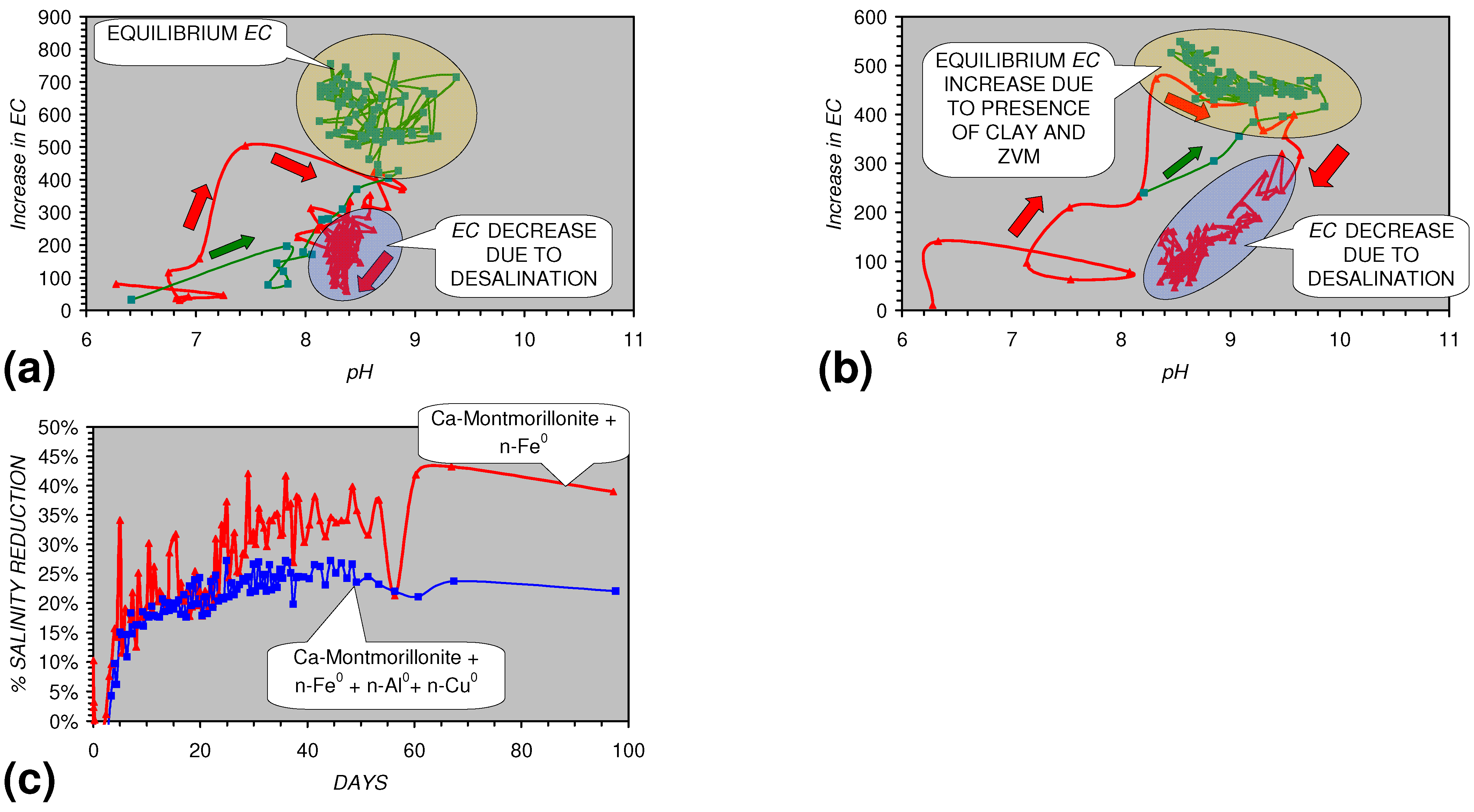
4.4.2. In Situ Aquifer Desalination

Aquifer desalination is traditionally water abstraction followed by surface based desalination using reverse (or forward) osmosis. However, this study has identified an alternative route for application in aquifers, which contain clays. Increasing groundwater pH by recirculation of aquifer water through m/n-ZVM (e.g., Figure 72b) (or by static diffusion) will decrease the cation exchange capacity, inter-layer spacing, bivalent (Fe + Mg + Ca) cation hydration shell level, while increasing the monovalent (e.g., Na + K) cation hydration shell levels of individual smectites contained within the aquifer [105]. An increase in pH from 7 to 9 (can double the smectite Na content (e.g., from 1.1 to 2.2 mmol g−1 smectite; 63.8 mg NaCl gm−1 smectite) and increase its hydrophilicity [86]. Consequently, increasing aquifer pH by ZVM treatment will decrease the concentration of Na+(aq) by forcing its integration into smectites, thereby reducing the salinization/sodicization of the aquifers.
This study includes photographic evidence associated with ZVM desalination in the presence of montmorillonite. For example, a freshwater sample (Figure 46) shows an increase in EC of 0.5 mS cm−1 (Figure 46) resulting from the addition of freshwater to Ca-montmorillonite + ZVM. However, the same clay-ZVM combination when added to saline water shows significantly smaller increases in EC of <0 to 0.2 mS cm−1 (e.g., Figure 41). The smaller EC increase results from Na adsorption in the clay interlayer space of 150 to >250 mg Na+ L−1. Figure 74 illustrates the observed relationship between EC, pH, time and proportion of Na+ in the saline water removed into the clay inter-layer space. The initial trend is an increase in EC until an equilibrium increase (associated with the clay) is reached at an increased pH. Substitution of clay cations by Na+ commences almost immediately and results in a continuing decrease in salinity over time. The variability associated with the salinity decrease decreases with the addition of n-Al0 and n-Cu0. Salinity decreases of 20–45% occurred within 10–50 days of treatment commencing (Figure 74).
Figure 74. Increase inEC μS cm−1 vs. pH. Arrows indicate directional change with time. Red/Blue = saltwater, Green = freshwater. (a) Ca-montmorillonite + n-Fe0 (Figure 6). (b) Ca Montmorillonite + n-Fe0 + n-Al0 + n-Cu0 (Figure 40, Figure 41 and Figure 46). (c) Salinity reduction as a function of time. Increase in EC is calculated as [EC of water – EC of water without Ca-montmorillonite + n-ZVM].
Sustainability 02 02988 g074
These experimental results indicate that ZVM can be used to desalinate or partially desalinate an aquifer. Total desalination is not required for irrigation water. A Wilcox Diagram [106,107,108] demonstrates (Figure 75) that ZVM, static diffusion treatment, can convert an aquifer from being unsuitable for irrigation to being suitable for irrigation in a treatment period lasting <50 days (Figure 74). The desalination can be observed from a plot of increase in EC vs. pH with the principal salination coinciding with the general decrease in pH (following its initial increase).
Figure 75. Desalination as a function of time (Figure 74c) plotted on a Wilcox diagram [106,107,108] identifying the suitability of the water for irrigation. Fe0 = red, n-Fe0 + n-Al0 +n-Cu0 = blue. EC = mS cm−1; Na = [Na + K]/[Ca + Mg + Na + K]. Na decreases with time.
Sustainability 02 02988 g075

4.4.3. Catalytic use of ZVM to both breakdown organic compounds and form new organic compounds

4.4.3.1. General Mechanism

Field tests have established that chloro-organics (e.g., TCE, DCE and vinyl chlorides (VC)) decompose in the presence of Fe0 to form ethene/ethane [6,7]. Experiments [109] have established that when aqueous CO2 is present (Figure 71) Fe catalyses the formation of simple polymerized hydrocarbons chains (alkanes) from reduced water. The basic process is:
Fe0 + H2O = OH + FeH+ − catalytic nuclei formation
Fe0 + H3O+ = Fe-H+ + H2O – catalytic nuclei formation
Fe-H+ + CO2 + 6H3O+ = Fe-CH3 + 8H2O – chain formation
Fe-CH3+ CO2 + 6H3O+ = Fe-CH2CH3 + 8H2O – chain growth
Fe-CH3+ CO2 + 6H3O+ = Fe-(CH2)2CH3 + 8H2O – chain growth
Fe-(CH2)2CH3 + 2H3O+ = Fe-H+ + 2H2O + CH3CH2CH3– chain termination
Catalytic nuclei formation reduces Eh and increases pH while chain propagation and growth involving CO2 results in an increase in pH. Isotope studies in organic contaminated water (containing aqueous CO2) confirmed the growth of hydrocarbons, but concluded that the bulk of the simple polymerized hydrocarbon products were sourced from the organic compounds destroyed by the Fe0 [110]. Some of the hydrocarbon products were derived from CO2 [110]. The catalytic intermediary was considered [110] to be FexCy. Experiments have established that TCE destruction is followed by the formation of simple alkanes [111]. However, >27% of the TCE carbon from chlorinated degradation remained sorbed to the iron surface until complete dechlorination is achieved [111], i.e., in a state of chain growth or catalytic nuclei formation.
Investigations [29,30,31,32] of low temperature (0–70 °C), medium pressure (10–50 MPa), alkane formation identified a similar decomposition and propagation route in saline water of the form:
ZVM + CxHyClz = ZVM-CaHbClc + … − catalytic nuclei formation
ZVM-CCl3 + CH4 = ZVM-CCl2CH3 + Cl + H+− chain growth
ZVM-CHCl2 + CH4 = ZVM-CH2CH3 + 2Cl− chain growth
ZVM-CH2CH3 + CH4 = ZVM-CH2CH2CH3 + 2H+− chain growth
ZVM-CHCl2 + 4H+ = ZVM-H+ + CH4 + 2Cl− chain termination
ZVM-CH2CH2CH3 + 2H+ = ZVM-H+ + CH3CH2CH3− chain termination
ZVM-CH2CH2CH3 + H+ = ZVM+ + CH3CH2CH3− chain termination
ZVM-CH2CH3 + ZVM-CH2CH3 + 2H+ = 2ZVM-H+ + CH3 CH2CH2CH3− chain termination
ZVM-CH2CH3 + ZVM-CH2CH3 = 2ZVM+ + CH3 CH2CH2CH3− chain termination
CH4 can be replaced by CxHy or CxHyClz or CxHyOz [29,30,31,32]. These and other associated observations [29,30,31,32] led to the development of a hypothesis that there is a direct reductive and polymerization interaction between organic chemicals/COx and ZVM to create catalytic growth/remediation nuclei. These interactions form nuclei of the generic form ZVM-(H+)n, ZVM-(O-H)n, ZVM-((CH)2)n, ZVM-CHn, ZVM-CHCl2, ZVM-CCl3, ZVM-CHCl, and ZVM-CH2Cl [28,29,30,31]. These nuclei act as loci for chain growth. For example:
ZVM + H+ = ZVM-H+
ZVM-H+ + CO2 = ZVM-COOH+
ZVM-H+ + CO2 + xH+ = ZVM-CHn+ + 2H2O
ZVM-H+ + CH4 = ZVM-CH3 + 2H+
ZVM-H+ + CO2 + 6H+ = ZVM-CH3 + 2H2O
ZVM reactions incorporating H+ or CO2 tend to increase pH by reducing the H3O+:[OH + HO2] ratio. Reactions incorporating CH4 tend to decrease pH. These decomposition routes are consistent with the ZVM studies [109,110,111]. ZVM+-C and ZVM-C nano-structures/nuclei [110] may form from the decomposition of Fe(CO)5 [29,31] and the discharge of super-critical CO2 into an aquifer [31,32]. During reductive decomposition Fe0 may also act as an electron shuttle (catalyst) whereby organic acids mediate electron transfer to O2, resulting in the OH radical-mediated oxidation of organic compounds through the Fenton Reaction [112].
All degradation routes involving ZVM as an intermediary will result in the formation of a residual base [29,30,31,32,109,110,111]. This base (e.g., ZVM+, ZVM-H+, ZVM-C, ZVM-CH, ZVM-CH2, ZVM-COx, ZVM-CxOyHz, ZVM-CH3, ZVM-CH2CH3 or ZVM-(CH2)2CH3) acts as a nuclei for chain growth in both an aqueous and gaseous environment [29,30,31,32,109,110]. In an aqueous environment, nuclei formation, the chain growth on the ZVM nuclei has been directly linked [31,32] to the aquifer Eh:pH (Figure 76).
ZVM chain growth is a binary process (Equations 77–79), which can be described by one or more polymerization ratios (PR) [29,30,31,32]. The polymerization ratio is calculated [29,30,31,32] as:
PR = Molar Abundance Cn+1Hm+2/ Molar abundance CnHm
The polymerization ratio does not describe the actual chain length associated with a ZVM-(CH2)nCH3 chain, it reflects the composition of the chain termination products [31]. For example:
ZVM- CH2CHCl2 + 4H+ = ZVM-CH3 + CH4 + 2Cl− chain termination
ZVM-CH2CH2CH3 + 2H+ = ZVM-CH2CH3 + CH4 − chain termination
The composition and molar distribution of the CxHy product for a specific pH is a function of Eh (Figure 76). The average product chain length decreases for a specific pH as the Eh decreases (Figure 76). This reflects an increase in H+ availability with decreasing Eh. The Kang-Choi electron shuttle model (KCESM) [111] provides a possible explanation for this observed phenomena which can occur under conditions of constant pH [31]. The KCESM [111] can be simplified [22,38] to:
Fe0 + 2H2O = 2OH + Fe-H2 = Fe2+ + 4H+ + O2(g)
This electron shuttle process decreases Eh (by production of OH) and subsequent decreases in pH (associated with the co-release of H+ and O2) are prevented by capture of H+ in organic chain formation/breaking reactions (Equations 77–81). This study (Figure 39) has confirmed that O2 release (Equation 82) is associated with negative Eh and that Eh declines are associated with the release of Fe ions. Both observations are consistent with the KCESM [111]. Chain growth theory [29,30,31,32] suggests that the primary control on the length and distribution of chain termination product is the availability of H+ (Figure 76), i.e., PR increases as the availability of H+ decreases (i.e., Eh increases). Similarly, (Equation 79) the formulation of Fe-H+ ions associated with dechlorination and organic compound decomposition [29] increases as H+ availability increases. This increase in H+ availability can be derived from either H3O+ or from the reductive breakdown of water (Equation 82).

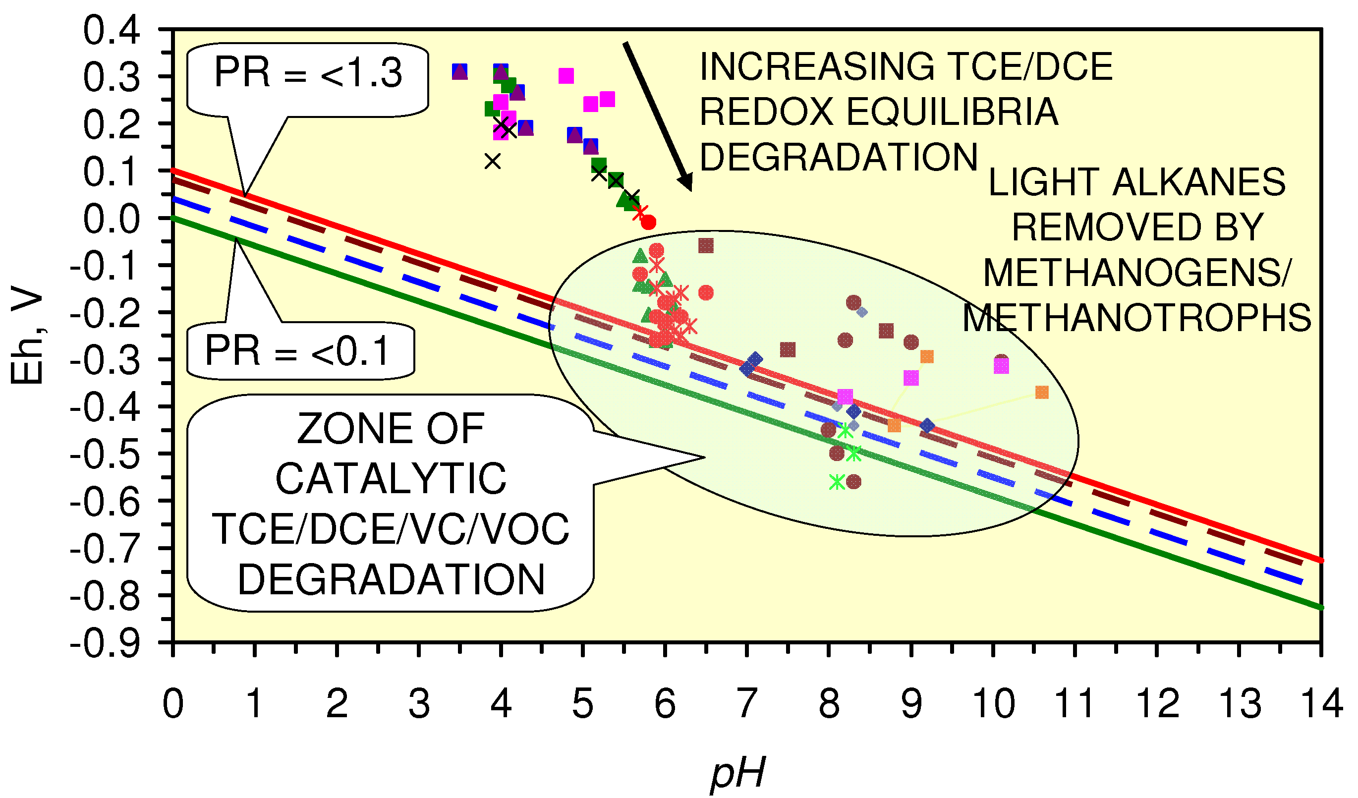
4.4.3.2. TCE, DCE, VC Remediation

TCE, DCE remediation projects utilizing ZVM [6,7] have sought to maximize remediation by maximizing the reduction in Eh. Low reductions in Eh are associated with remediation associated with the redox equilibria relationship (Figure 71, Equations 75, 76] between TCE:DCE:VC with VC’s becoming progressively more abundant as Eh decreases [6]. Substantial Eh reductions move the redox environment into the zone (Figure 76) where Fe catalytic nuclei are active [31,32]. Within this zone (Figure 76) the majority of TCE, DCE, and VC are reduced to methane and ethene/ethane [6,7]. Methanotrophs may remove the methane and light hydrocarbon products within the aquifer within this environment. This general pattern of remediation is illustrated (Figure 77) for a number of pilot n-ZVM injection TCE remediation projects [6]. This analysis (Figure 77) demonstrates that a redox plot can identify the dominant mechanistic control on the TCE degradation within the aquifer during a treatment program. The highest levels of TCE remediation are obtained within the zone (following remediation) where PR < 1.3 (Figure 77) and pH is between 5 and 10.

4.4.3.3. Optimization of TCE, DCE, VC Remediation

The redox analysis (Figure 77) has identified that the preferred aquifer Eh for Fe-catalytic TCE remediation has a PR < 1.3. This study has demonstrated (Figure 3) that if n-ZVM is injected into the aquifer, then the aquifer permeability will decline with time due to a mixture of mineralization and pore occlusion associated with O2 formation.n-ZVM injection volumes tend to be focused around the injection well. The m-ZVM analysis has established that redox alteration by recirculation can deliver a high concentration of catalytic Fe(a−n)+H ions into the aquifer while progressively reducing its Eh. Recirculation allows an even distribution of both the Eh reduction and catalytic Fe(a−n)+H ion distribution within the aquifer. This may allow a remediation program to control the rate and duration of the TCE remediation, without leaving a legacy of n-ZVM residues within the aquifer. A typical n-ZVM remediation program will target groundwater mounds/plumes with a volume of <1,000 m3. Figure 72 has demonstrated that m-ZVM recirculation can modify the Eh and pH of a 10,000 m3 aquifer. Increasing the recirculation rate to 1000 m3 d−1 would allow the redox environment of a 100,000 m3 polluted aquifer to be controlled. The modeled changes in Eh and pH over a 400 day and 450 day recirculation period are shown relative to the redox fences associated with the polymerization of CxHy (Figure 76). These indicate that a program of surface based pore water recirculation through m-ZVM or n-ZVM over a period 400–450 days will adjust the aquifer redox environment into the region associated with active reduction and reformulation of TCE, DCE, VC (Figure 77). This approach allows the application of recirculation to remove specific pollutants. Following their removal the recirculation treatment can cease.
Figure 76. Redox fences associated with the polymerization of CxHy. PR = Polymerization ratio (Equation 79). (a) Redox fences [30,31]. (b) Aquifer recirculation program: Duration 0–400 days. (c) Aquifer recirculation program: Duration 0–450 days. SV = 100; self-sealing ground water mound contains 10,000 m3; Recirculation rate = 100 m3 d−1.
Sustainability 02 02988 g076aSustainability 02 02988 g076b
Figure 77. Pilot n-ZVM TCE Remediation. Data from [6]. Each color symbol represents data from a different measurement point in TCE polluted GWMs following n-ZVM treatment. Redox fences [31,32].
Sustainability 02 02988 g077

4.4.3.4. Cathodic Hydrogen Release during TCE, DCE, VC Remediation

It is frequently reported that H2(g) release is associated with Fe0 [113]. The evidence is typically indirect (e.g., enhanced presence of H2 consuming methanotrophs [114]). Small quantities of H2 discharge have been measured shortly after engineered n-Fe0 particles are placed in water [113]. This engineered n-Fe0 is manufactured from the reduction of a ferrous iron with sodium borohydride reduction [113]. The implied reaction associated with Fe0 from bioremediation studies (associated with chloro-hydrocarbon remediation studies) are summarized in Equation 55 [78,115,116,117]. In this study no free H2 was observed. The Eh, pH and EC data and photographs confirm that H2(g) is not released, and that the released gas is actually O2. All the n-Fe0 used in this study was commercial grade high purity iron powder used in automobile paint manufacture. It is produced by grinding high purity iron. There may be a difference in the catalytic interaction with water of precipitated iron nano-particles and nano-particles created by grinding crystalline iron.
Fragmentation analysis [118] has demonstrated that Fe[H2O] can produce O2, H2, H, or OH. This analysis has established that ZVM results in an oscillation in Eh and pH with time (e.g., Figure 14, Figure 61 and Figure 69). The Bray-Liebhafsky oscillation (originally recognized for iodides) results from the continual equilibrium oscillation [119,120] between two reactions
MOx + nH+ + mOH = M0 + xH2O + yO2(g)
M0 + mOH = MOx + nH+ + xH2O
M = iodine or metal. In the oscillations observed in this study M0 = ZVM and MOx = ZVM – Ox or ZVM-OH. The oscillation is between an absorbent + reductive phase (Equation 83) and a sorbent + oxidation phase (Equation 84). This dual function oscillation allows n-Fe0 (and m-Fe0) to provide an efficient and unique solution for the separation and transformation of metal ions and the transformation of environmental contaminants [121]. This dual function also allows Fe0 to be an effective chemical filtrate for H2S and an effective reducer of CO, CO2, CxHyOz, and an intermediary for the formation of CxHy. Fe[H2O] assumes the structure H-Fe-OH [118]. This allows for an oscillation between the generic reactions:
Generic reduction ZVM Oscillation involving –Fe-OH(s) or Fe-OH(aq).
zFeOH + nH+ + mOqH + kH2O + cFedOb = pFe0 + gFe-H+ + xH2O + yO2(g) + jOqH
O2 degassing, Eh reduction, and pH increase or decrease
Generic oxidation ZVM Oscillation involving Fe0 or Fe-H+
pFe0 + gFe-H+ + xH2O + rOqH + cFedOb = zFeOH + nH+ + mOqH + hFe-H++ jH2(g)
H+ ion or H2(g) formation, Eh and pH increase or decrease
Product selectivity in each oscillation can be controlled by chemically engineering the ZVM and by adjusting the adjacent mineral/ZVM composition. This study has demonstrated that Fe0 oscillation selectivity can be altered by the addition of Cu0, Al0 and Ca-montmorillonite. High O2(g) selectivity (Equation 85) is provided by the addition of Al0 + Cu0 (Figure 8) and Ca-montmorillonite (Figure 5, 6). Figure 8 demonstrates a transition from a hydrophophyllic surface (Figure 8e) through an intermediate wetness surface (Figure 8a) through to a hydrophobic surface (Figure 8f) [122]. The size of the O2 bubbles and their discharge intensity increases as the Eh reduces.
Fe0 and Fe0 + Cu0 (Figure 7) show a lower initial selectivity towards O2 degassing and a preference for OxH formation during the reductive phase. This is demonstrated by the higher equilibrium pH for Fe0 when compared with Fe0 + Cu0 + Al0. However when the equilibrium oscillations lower pH, selectivity switches from H2O formation to O2 degassing (Equation 85, Figure 7). The water-n-Fe0 interface gradually accumulates Fe-hydroxides (Equation 86, Figure 7) indicating a preferred selectivity of hydroxides rather than H2 formation during the oxidation phase of the oscillation (Equation 86). Engineered n-Fe0 can be designed to have a preferred selectivity for H2(g) during the oxidation phase [113]. The nano-structure can be engineered [121] to have an outer shell focusing on oxidation reactions (Equation 86) and an inner shell focusing on reduction reactions (Equation 85). A similar macro-structure is illustrated in Figure 7a, b) at the water-ZVM interface.

4.4.3.5. Relative Reaction Rate for TCE, DCE, VC Remediation

ZVM studies tend to ignore the intermediate oxides/hydroxides produced by Equation 86 (e.g., hematite, magnetite, goethite and the interaction of equilibrium Fe-oxides. These have been demonstrated to be highly reactive reducing agents (Equation 85) [29,30,31,32,123,124]. Reaction rate is a function of both catalyst surface area (which increases with decreasing particle size) and the presence of promoters [115,123,124]. The presence of promoters can result in a substantial acceleration in reaction rate. This can result in the reaction rate for m-ZVM with promoters (e.g., Al, K, Ca, Cu, Na, Mg, Mn, Pt), exceeding the reaction rate for n-ZVM without promoters.
The static diffusion analyses have established that the change from the equilibrium state without ZVM to an equilibrium state with ZVM follows a trajectory. This trajectory involves an initial decrease in Eh (for the NH4+:NOx redox fence) followed by a later increase in pH (e.g., Figure 14). This latter change shifts the redox environment into the Fe2O3 stability zone and away from both the NH4+:NOx redox fence and the redox fence associated with catalytic TCE/DCA/VC/VOC degradation (Figure 74 and Figure 75). The design of an effective remediation program needs to consider whether it is desirable to stabilize the treated water at location along the trajectory, or in an equilibrium area. Static diffusion associated with PRB’s and n-ZVM injection programs will always stabilize the redox environment in the equilibrium oscillation area. n-ZVM will reach the equilibrium oscillation zone over a shorter time span than m-ZVM and may be able to achieve the transition with a smaller change in Eh.
This study has established that the slower reaction rate associated with m-ZVM can be used to stabilize high flow rates of treated water on the trajectory. This allows both continuous treatment of flowing water and continuous recirculation of flowing water through m-ZVM to significantly lower Eh with only minor changes in pH. This allows for more effective high volume remediation of TCE/DCA/VC/VOC and nitrates than can be achieved by using n-ZVM.

5. Conclusions

The experimental regression equations associated with m-ZVM provide a sustainable basis for the quantitative prediction of ZVM remediation of aquifers, both during the remediation design phase and following installation. The regression modeling allows direct comparison between actual aquifer remediation performance and the design parameters of the remediation program.
Sustainable development is an ideal political goal in most cultural environments. In this context sustainable development requires the remediation of aquifers (due to industrial/mining/agricultural pollutants) to allow continued abstraction, remediation of polluted ground (associated with brownfield and other sites) and desalination of aquifers to provide water for irrigation and domestic/industrial consumption. It also requires the ability to create a sustainable solution to the provision of water supply following anthropogenic/natural disasters.
The four broad categories (meteorological, hydrological, agricultural and socio-economic) of drought all result in depletion of stored water resources [125]. This depletion may be associated with reduced dilution of mineral leaching from the host rock into the aquifer or reduced dilution of anthropogenic pollutants entering an aquifer. The resultant increase in mineral concentrations and pollutants in the aquifer water may, in turn, reduce the availability of water which can be used for agricultural (irrigation) or drinking purposes. Climate change will present additional problems by potentially increasing the incidence of meteorological and hydrological drought in some areas. The socio-economic challenge resulting from this increased stress on scarce water resources will require that the remediation of sub-standard and polluted water resources provides a sustainable solution. Increasingly sustainable energy policies require the replacement of fossil fuel powered treatment works and energy intensive treatment systems with less energy intensive systems. This study has identified that m-ZVM can be used to design and provide low cost, low technology, low energy requirement, sustainable, water treatment and In Situ aquifer remediation (for small and large water volumes) to remove anthropogenic and natural pollutants. Specifically the study has demonstrated that geoengineering of aquifers using ZVM treatment can reverse the sodification/salinization of aquifers, reverse aquifer nitrification and create the required redox environment for controlled catalytic destruction of organic pollutants (including TCE, DCE, VC, VOC) in the aquifer. These observations suggest that a sustainable water treatment program can counter the adverse effects of both drought and socio-economic activities on water quality in the aquifer. This, in turn, allows ZVM treatment of water to increase the available global water supply for irrigation and drinking water from existing aquifers and prolong abstraction from aquifers which are adversely affected by climate change and socio-economic factors.

Acknowledgements

The two reviewers are thanked for their helpful and constructive comments on an earlier draft.

References

  1. Antia, D.D.J. Formation and control of self-sealing high permeability groundwater mounds implications for suds and sustainable pressure mound management. Sustainability 2009, 1, 855–923. [Google Scholar] [CrossRef]
  2. Antia, D.D.J. Interacting Infiltration Devices (Field Analysis, Experimental Observation and Numerical Modeling): Prediction of seepage (overland flow) locations, mechanisms and volumes—Implications for SUDS, groundwater raising projects and carbon sequestration projects. In Hydraulic Engineering: Structural Applications, Numerical Modeling and Environmental Impacts, 1st ed.; Hirsch, G., Kappel, B., Eds.; Nova Science Publishers: Hauppauge, NY, USA, 2010; pp. 85–156. [Google Scholar]
  3. Merly, C.; Lerner, D.N. Remediation of Chlorinated Organic Contaminants in Fractured Aquifers Using Zero-Valent Metal: Report on Laboratory Trials; R&D Technical Report P2-182/TR; Environment Agency: Bristol, UK, 2002; p. 105. [Google Scholar]
  4. Dolfing, J.; Van Eekert, M.; Seech, A.; Vogan, J.; Mueller, J. In Situ chemical reduction (ISCR) technologies: Significance of low Eh reactions. Soil Sed. Contam. 2008, 17, 63–73. [Google Scholar] [CrossRef]
  5. Fiore, S.; Zanetti, M.C. Preliminary tests concerning zero-valent iron efficiency in organic pollutants removal. Am. J. Environ. Sci. 2009, 5, 555–560. [Google Scholar] [CrossRef]
  6. Gavaskar, A.; Tatar, L.; Condit, W. Cost and Performance Report: Nanoscale Zero-Valent Iron Technologies for Source Remediation; Contract Report CR-05-007-ENV; NAVFAC Naval Facilities Engineering Command, US Navy Engineering Services Center: Port Hueneme, CA, USA, 2005; p. 44. [Google Scholar]
  7. Gavaskar, A.; Bhargava, M.; Condit, W. Cost and Performance Report for a Zero-valent Iron (ZVI) Treatability Study at Naval Air Station North Island; Technical Report TR-2307-ENV; Naval Facilities Engineering Command (NAVFAC), US Navy Engineering Services Center: Port Hueneme, CA, USA, 2008. [Google Scholar]
  8. Pula, R.W.; Paul, C.J.; Powell, R.M. The application of In Situ permeable reactive (zero-valent iron) barrier technology for the remediation of chromate-contaminated groundwater: A field test. App. Geochem. 1999, 14, 989–1000. [Google Scholar] [CrossRef]
  9. Ludwig, R.D.; Smyth, D.J.; Blowes, D.W.; Spink, L.E.; Wilkin, R.T.; Jewett, D.G.; Weisener, C.J. Treatment of arsenic, heavy metals, and acidity using a mixed ZVI-compost PRB. Environ. Sci. Technol. 2009, 43, 1970–1976. [Google Scholar] [CrossRef] [PubMed]
  10. Phillips, D.H.; Van Noolen, T.; Basfianens, L.; Russell, M.I.; Dickson, K.; Plant, S.; Ahad, J.M.; Newton, T.; Elliot, T.; Kalin, R.M. Ten year performance evaluation of a field-scale zero-valent iron permeable reactive barrier installed to remediate trichloroethene contaminated groundwater. Environ. Sci. Technol. 2010, 44, 3061–3069. [Google Scholar]
  11. Komnitsas, K.; Bartzas, G.; Fytas, K.; Paspaliaris, L. Long-term efficiency and kinetic evaluation of ZVI barriers during clean-up of copper containing solutions. Min. Engrg. 2007, 20, 1200–1209. [Google Scholar]
  12. Warrender, R. Remediation of Circum-Neutral Metal Mine Drainage Using Laboratory Scale Permeable reactive Barriers; Ph.D. Thesis, University of Aberystwyth, Aberystwyth, UK, 2009.
  13. Fatemi, F.; Liu, L.; Mahabadi, O.K.; Satish, M. Investigating the effect of implementing heating rods within a ZVI-PRB to enhance performance, improve design and reduce costs. Water Air Soil Poll. 2008, 190, 231–243. [Google Scholar] [CrossRef]
  14. Higgins, M.R.; Olson, T.M. Life-cycle case study comparison of permeable reactive barrier versus pump-and-treat remediation. Environ. Sci. Technol. 2009, 43, 9432–9438. [Google Scholar] [CrossRef] [PubMed]
  15. Johnson, T.; O’Brien, J.; Nurmi, T. Mineral precipitation up gradient from a zero-valent iron permeable reactive barrier. Ground Water Mon. Remid. 2008, 28, 56–64. [Google Scholar] [CrossRef]
  16. McElroy, B.; Keith, A.; Glasgow, J.; Dasappa, S. The use of zero-valent iron injection to remediate groundwater: Results of a pilot test at the Marshall Space Flight Center. Remediation J. 2003, 13, 145–153. [Google Scholar] [CrossRef]
  17. Joo, S.H.; Cheng, F. Nanotechnology for Environmental Remediation; Springer: Hiedelberg, Germany, 2006; p. 166. [Google Scholar]
  18. Vaughan, P.R. Observations on the behaviour of clay fill containing occluded air bubbles. Geotechnique 2003, 53, 265–272. [Google Scholar] [CrossRef]
  19. Smoltczyk, V. Geotechnical Engineering Handbook: Fundamentals; Wiley: Chichester, UK, 2002; Volume 1. [Google Scholar]
  20. Smith, P.G.C. Numerical Analysis of Infiltration into Partially Saturated Soil Slopes ; Ph.D. Thesis, University of London, London, UK, 2003.
  21. Valdes, J.R.; Santamarina, J.C. Particle clogging in radial flow: Microscale mechanisms. SPE J. 2006, 11, 193–198. [Google Scholar] [CrossRef]
  22. Wiekowski, A. Interfacial Electrochemistry: Theory, Experiment and Applications; CRC: London, UK, 1999; p. 992. [Google Scholar]
  23. Greenwood, N.N.; Earnshaw, A. Chemistry of the Elements; Pergamon: Oxford, UK, 1990. [Google Scholar]
  24. Kim, E.H.; Chung, D.Y.; Park, J.H.; Yoo, J.H. Dissolution of oxylate precipitate and destruction of oxalate ion by hydrogen peroxide in nitric acid solution. J. Nuc. Sci. Technol. 2000, 37, 601–607. [Google Scholar] [CrossRef]
  25. Astrus, D. Organometallic Chemistry and Catalysis; Springer: London, UK, 2007; p. 608. [Google Scholar]
  26. Huang, K.H. Catalysis mechanism and kinetic equation of ammonia synthesis on doubly-promoted iron catalysts. Sci. China Ser. A 1981, 24, 800–813. [Google Scholar]
  27. McKee, M.L. Ab Initio study of the interaction of Fe, Fe+, and HFe with H, CH, CH2, CH3, and C5H5. J. Am. Chem. Soc. 1990, 112, 2601–2607. [Google Scholar] [CrossRef]
  28. Yamakawa, K.; Nishimuara, R. Hydrogen permeation of carbon steel in weak alkaline solution containing hydrogen sulphide and cyanide ion. Corrosion 1999, 56, 24–30. [Google Scholar] [CrossRef]
  29. Antia, D.D.J. Oil polymerisation and fluid expulsion from low temperature, low maturity, over pressured sediments. J. Petrol. Geol. 2008, 31, 263–282. [Google Scholar] [CrossRef]
  30. Antia, D.D.J. Low temperature oil polymerisation and hydrocarbon expulsion from continental shelf and continental slope sediments. Indian J. Petrol. Geol. 2009, 16, 1–30. [Google Scholar]
  31. Antia, D.D.J. Polymerisation Theory—Formation of hydrocarbons in sedimentary strata (hydrates, clays, sandstones, carbonates, evaporites, volcanoclastics) from CH4 and CO2: Part I: Polymerisation concepts, kinetics, sources of hydrogen, and redox environment. Indian J. Petrol. Geol. 2009, 17, 49–86. [Google Scholar] Part II: Formation and Interpretation of Stage 1 to Stage 5 Oils. Indian J. Petrol. Geol. 2009, 17, 11–70. Part III: Hydrocarbon expulsion from the hydrodynamic flow regimes contained within a generating pressure mound. Indian J. Petrol. Geol. 2010, 18. in press. Part IV: Polymerisation modelling of sequestered carbon dioxide and waste organic liquids to hydrocarbons. Indian J. Petrol. Geol. 2010, 18. in press.
  32. Antia, D.D.J. Polymerisation Theory (the catalytic formation of oil from CO2 and CH4): Application of an Accelerated Geological Process to Remove Carbon Oxides from Flue Gases and use Carbon Oxide Sequestration to Produce Oil in Sedimentary Sequences. J. Appl. Geochem. 2010, 12. in press. [Google Scholar]
  33. Lindberg, R.D.; Runnells, D.D.D. Ground Water Redox Reactions: An analysis of the equilibrium state applied to Eh measurements and geochemical modeling. Science 1984, 225, 925–927. [Google Scholar] [CrossRef] [PubMed]
  34. Stefansson, A.; Arnorsson, S.; Sveinbjornsdorrir, A.E. Redox reactions and potentials in natural waters at disequilibrium. Chem. Geol. 2005, 221, 289–311. [Google Scholar] [CrossRef]
  35. Grenthe, I.; Stumm, W.; Laaksuharju, M.; Nilsson, A.C.; Wikberg, P. Redox potentials and redox reactions in deep groundwater systems. Chem. Geol. 1992, 98, 131–150. [Google Scholar] [CrossRef]
  36. Washington, J.W.; Endale, D.M.; Samarkina, L.P.; Chappell, K.E. Kinetic control of oxidation state at thermodynamically buffered potentials in subsurface waters. Geochim. Cosmochim. Acta 2004, 68, 4831–4842. [Google Scholar] [CrossRef]
  37. Ebbing, D.D.; Gammon, S.D. General Chemistry; Houghton Mifflin: Boston, MA, USA, 1999. [Google Scholar]
  38. Bokare, A.D.; Choi, W. Zero-valent aluminium for oxidative degradation of aqueous organic pollutants. Environ. Sci. Technol. 2009, 43, 7130–7135. [Google Scholar] [CrossRef] [PubMed]
  39. Mulder, M. Basic Principles of Membrane Technology; Kluwer Academic Publishers: Dordrecht, Germany, 1996. [Google Scholar]
  40. Junyapoon, S. Use of zero-valent iron for waste water treatment. KMITL. Sci. Tech. J. 2005, 5, 587–595. [Google Scholar]
  41. Hao, Z.W.; Xu, X.H.; Wang, D.H. Reductive denitrification of nitrate by scrap iron filings. J. Zhejang Univ. Sci. B 2005, 6, 182–186. [Google Scholar] [CrossRef]
  42. Hao, Z.W.; Xu, X.H.; Jin, J.; He, P.; Liu, Y.; Wang, D.H. Simultaneous removal of nitrate and heavy metals by iron metal. J. Zhejang Univ. Sci. B 2005, 6, 307–310. [Google Scholar] [CrossRef]
  43. Ottley, C.J.; Davison, W.; Edmunds, W.M. Chemical catalysis of nitrate reduction by iron (II). Geochim. Cosmochim. Acta 1997, 61, 1819–1828. [Google Scholar] [CrossRef]
  44. Young, G.K.; Bungay, H.R.; Brown, L.M.; Parsons, W.A. Chemical reduction of nitrate in water. J. Water Poll. Cont. Fed. 1964, 36, 395–398. [Google Scholar]
  45. Liou, Y.H.; Lo, S.L.; Lin, C.J.; Kuan, W.H.; Weng, S.C. Chemical reduction of unbuffered nitrate solution using catalysed and uncatalyzed nanoscale iron particles. J. Hazard. Mat. 2005, B127, 102–110. [Google Scholar] [CrossRef]
  46. Liou, Y.H.; Lo, S.L.; Lin, C.J.; Kuan, W.H.; Weng, S.C. Effects of iron surface pretreatment on kinetics of aqueous nitrate reduction. J. Hazard. Mat. 2005, B126, 189–194. [Google Scholar] [CrossRef]
  47. Liou, Y.H.; Lo, S.L.; Lin, C.J.; Kuan, W.H.; Weng, S.C. Methods for accelerating nitrate reduction using zero-valent iron at near neutral pH: Effects of H2 reducing pretreatment and copper deposition. Environ. Sci. Technol. 2005, 39, 9643–9648. [Google Scholar] [CrossRef] [PubMed]
  48. Choi, J.; Batchelor, B. Nitrate reduction by fluoride green rust modified with copper. Chemosphere 2008, 70, 1106–1116. [Google Scholar] [CrossRef]
  49. Chen, Y.M.; Li, C.W.; Chen, S.S. Fluidised zero-valent iron bed reactor for nitrate removal. Chemosphere 2005, 59, 753–759. [Google Scholar] [CrossRef] [PubMed]
  50. Huang, C.P.; Wang, H.W.; Chiu, P.C. Nitrate reduction by metallic iron. Water Res. 1998, 32, 2257–2264. [Google Scholar] [CrossRef]
  51. Huang, Y.H.; Zhang, T.C.; Shea, P.J.; Comfort, S.D. Effects of oxide coatings on nitrate reduction by iron metal. J. Environ. Qual. 2003, 32, 1306–1315. [Google Scholar] [CrossRef] [PubMed]
  52. Buresh, R.J.; Moraghan, J.T. Chemical reduction of nitrate by ferrous iron. J. Environ. Qual. 1976, 5, 320–325. [Google Scholar] [CrossRef]
  53. Rakshit, S.; Matocha, C.J.; Haszler, G.R. Nitrate reduction in the presence of wustite. J. Environ. Qual. 2005, 34, 1286–1292. [Google Scholar] [CrossRef] [PubMed]
  54. Westerhoff, P. Reduction of nitrate, bromate, and chlorate by zero-valent iron (Fe0). J. Envir. Engrg. 2003, 129, 10–16. [Google Scholar] [CrossRef]
  55. Huang, Y.H.; Zhang, T.C. Nitrite reduction and formation of corrosion coatings in zero-valent iron systems. Chemosphere 2006, 64, 937–943. [Google Scholar] [CrossRef] [PubMed]
  56. Rakshit, S.; Matocha, C.J.; Coyne, M.S. Nitrite reduction by siderite. Soil. Sci. Soc. Am. J. 2008, 72, 1070–1077. [Google Scholar] [CrossRef]
  57. Cohen, E.L.; Patterson, B.M.; McKinley, A.J.; Prommer, H. Zero-valent iron remediation of a mixed brominated ethene contaminated groundwater. J. Contam. Hydrol. 2009, 103, 109–118. [Google Scholar] [CrossRef] [PubMed]
  58. Wer, Y.T.; Wu, S.C.; Chou, C.M.; Che, C.H.; Tsai, S.M.; Lien, H.L. Influence of nanoscale zero-valent iron on geochemical properties of groundwater and vinyl chloride degradation: A field case study. Water Res. 2010, 44, 131–140. [Google Scholar] [CrossRef] [PubMed]
  59. Nurmi, J.T.; Tratnyek, P.G.; Johnson, R.L.; O’Brien, R. Reduction of TNT and RDX by core material from an iron permeable reactive barrier. In Remediation of Chlorinated and Recalcitrant Compounds; Sass, B.M., Ed.; Battelle: Columbus, OH, USA, 2008. [Google Scholar]
  60. Lee, J.Y.; Lee, K.L.; Youm, S.Y.; Lee, M.R.; Kamala-Kannan, S.; Oh, B.T. Stability of multi-permeable reactive barriers for long term removal of mixed contaminants. Bull. Environ. Cont. Tox. 2010, 84, 250–254. [Google Scholar] [CrossRef]
  61. Chang, M.C.; Kang, H.Y. Remediation of pyrene-contaminated soil by synthesized nanoscale zero-valent iron particles. J. Environ. Sci. Health 2009, 44, 576–582. [Google Scholar] [CrossRef]
  62. Katsenovch, Y.P.; Miralles-Wilhelm, F.R. Evaluation of nanoscale zerovalent iron particles for trichloroethene degradation in clayey soils. Sci. Total Environ. 2009, 407, 4986–4993. [Google Scholar] [CrossRef] [PubMed]
  63. Lo, I.M.C.; Lai, K.C.K. Zero-Valent Iron Reactive Materials for Hazardous Waste and Inorganics Removal; American Society of Civil Engineers: Reston, VA, USA, 2007; p. 340. [Google Scholar]
  64. Li, W.G.; Zhang, W.X. Sequestration of metal cations with zerovalent iron nanoparticles—A study with high resolution X-ray photoelectron spectroscopy (HR-XPS). J. Phys. Chem. C 2007, 111, 6939–6946. [Google Scholar] [CrossRef]
  65. Sun, H.; Wang, L.; Zhang, R.; Sui, J.; Xu, G. Treatment of groundwater polluted by arsenic compounds by zero-valent iron. J. Hazard. Mat. 2006, 129, 297–303. [Google Scholar] [CrossRef]
  66. Alshaebi, F.Y.; Yaacob, W.Z.W.; Samsuldin, A.R. Sorption on zero-valent iron (ZVI) for arsenic removal. Eur. J. Sci. Res. 2009, 33, 214–219. [Google Scholar]
  67. Zhang, Y.; Wang, J.; Amrhein, C.; Frankenberger, W.T., Jr. Removal of selanate from water by Zerovalent iron. J. Environ. Qual. 2005, 334, 487–495. [Google Scholar] [CrossRef]
  68. Fiedor, J.N.; Bostick, W.D.; Jarabek, R.J.; Farrell, J. Understanding the mechanism of uranium removal from groundwater by zero-valent iron using X-ray photoelectron spectroscopy. Environ. Sci. Technol. 1998, 32, 1466–1473. [Google Scholar] [CrossRef]
  69. Rangsivek, R.; Jekel, M.R. Removal of dissolved metals by zero-valent iron (ZVI): Kinetics, equilibria, processes and implications for storm runoff treatment. Water Res. 2005, 39, 4153–4163. [Google Scholar] [CrossRef] [PubMed]
  70. Stapanajaru, T.; Comfort, S.D.; Shea, P.J. Enhancing metolachlor destruction rates with aluminum and iron salts during zerovalent iron treatment. J. Environ. Qual. 2003, 32, 1726–1734. [Google Scholar] [CrossRef] [PubMed]
  71. Satapanajaru, T.; Anurakpongsatorn, P.; Pengthamkeerati, P.; Boparai, H. Remediation of atazine-contaminated soil and water by nano zerovalent iron. Water Air Soil Pol. 2008, 192, 349–359. [Google Scholar] [CrossRef]
  72. Misstear, B.; Banks, D.; Clark, L. Water Wells and Boreholes; Wiley: Chichester, UK, 2006. [Google Scholar]
  73. Geological Survey Japan. Atlas of Eh-pH Diagrams; Open File Report No. 419; National Institute of Advanced Industrial Science and Technology: Naoto, Takeno, Japan, 2005. [Google Scholar]
  74. Stephanov, M.F.; Novakovskaya, Y.V. Rate constants of atomic hydrogen formation in H3O+(H2O)n + e = H + (H2O)n gas-phase. Russian J. Phys. Chem. A. Focus Chem. 2009, 83, 1502–1510. [Google Scholar] [CrossRef]
  75. Yeh, L.I.; Okumura, M.; Myers, J.D.; Price, J.M.; Lee, Y.T. Vibrational spectroscopy of the hydrated hydronium cluster ions H3O+ · (H2O)n (n = 1,2,3). J. Chem. Phys. 1989, 91, 7319–7330. [Google Scholar] [CrossRef]
  76. Conway, B.E.; Tessier, D.F. Comparison of the kinetics of cathodic H2 evolution from the unhydrated H3O+ ion and its hydrated form H9O4+: Frequency factor effects and modes of activation. J. Chem. Kin. 2004, 13, 925–944. [Google Scholar] [CrossRef]
  77. Mabourki, R.; Ibrahim, Y.; Xie, E.; Meof-Ner (Mautner), M.; El-Shali, M.S. Clusters of the hydronium ion (H3O+) with H2, N2 and CO molecules. Chem. Phys. Let. 2006, 424, 257–263. [Google Scholar] [CrossRef]
  78. Zolla, V.; Sethi, R.; Molfetta, A.D. Performance assessment and monitoring of a permeable reactive barrier for the remediation of a contaminated site. Am. J. Environ. Sci. 2007, 3, 158–167. [Google Scholar] [CrossRef]
  79. Kamer, G.; Osta, C.; Mitsui, S.; Shibata, M.; Shinozaki, T. Fe(II)-Na ion exchange at interlayers of smectite: Adsorption-desorption experiments and a natural analogue. Engrg. Geol. 1999, 54, 15–20. [Google Scholar] [CrossRef]
  80. Drame, H. Cation exchange and pillaring of smectites by aqueous Fe nitrate solutions. Clays Clay Min. 2005, 53, 335–347. [Google Scholar] [CrossRef]
  81. Frini, N.; Crespin, M.; Trabelsi, M.; Messad, D.; Van Damme, H.; Bergaya, F. Preliminary results on the properties of pillared clays by mixed Al-Cu solutions. Appl. Clay Sci. 1997, 12, 281–292. [Google Scholar] [CrossRef]
  82. Fujita, S.I.; Bhanage, B.M.; Aoki, D.; Ochial, Y.; Iwasa, N.; Arai, M. Mesoporous smectites incorporated with alkali metal cations as solid base catalysts. Appl. Catal. A: Gen. 2006, 313, 151–159. [Google Scholar] [CrossRef]
  83. Kloprogge, J.T. Synthesis of smectites and porous pillared clay catalysts: A review. J. Por. Mat. 1998, 5, 5–41. [Google Scholar] [CrossRef]
  84. Martin-Luengo, M.A.; Martins-Carvalho, H.; Ladriere, J.; Grange, P. Fe(III)-pillared montmorillonites: Preparation and characterisation. Clay Min. 1989, 24, 495–504. [Google Scholar] [CrossRef]
  85. Rightor, E.G.; Tzou, M.S.; Pinnavaia, T.J. Iron oxide pillared clay with large gallery height: Synthesis and properties as a Fischer-Tropsch catalyst. J. Catal. 1991, 130, 29–40. [Google Scholar] [CrossRef]
  86. Zhu, H.Y.; Yamanaka, S. Molecular recognition of Na-loaded alumina pillared clay. J. Chem. Soc. Faraday Trans. 1997, 93, 477–480. [Google Scholar] [CrossRef]
  87. Chatterjee, A. Application of localized reactivity index in combination with periodic DFT calculation to rationalise the swelling mechanism of clay type in-organic material. J. Chem. Sci. 2005, 117, 533–539. [Google Scholar] [CrossRef]
  88. Soakaway Design. Digest 365; Building Research Establishment: Watford, UK, 1991.
  89. Flood Studies Report; Institute of Hydrology: Wallingford, UK, 1993; Volume 6.
  90. Flood Estimation Handbook; Institute of Hydrology: Wallingford, UK, 1999; Volume 5.
  91. Martin, P.; Turner, B.; Waddington, K.; Pratt, C.; Campbell, N.; Payne, J.; Reed, B. Sustainable Urban Drainage Systems: Design Manual for Scotland and Northern Ireland; CIRIA Report No. C521; CIRIA: London, UK, 2000. [Google Scholar]
  92. Wilson, S.; Bray, R.; Cooper, P. Sustainable Drainage Systems: Hydraulic, Structural and Water Quality Advice; CIRIA Report No. C609; CIRIA: London, UK, 2004. [Google Scholar]
  93. Woods Ballard, B.; Kellagher, R.; Martin, P.; Jefferies, C.; Bray, R.; Shaffer, P. The SUDS Manual; CIRIA Report No. C697; CIRIA: London, UK, 2007. [Google Scholar]
  94. Design Manual for Roads and Bridges; Design of Soakaways, Highways Agency, Stationary Office: London, UK, 2006; Volume 4.
  95. Youngs, E.G. The analysis of groundwater seepage in heterogenous aquifers. Hydrol. Sci. 1980, 25, 155–165. [Google Scholar]
  96. Antia, D.D.J. Prediction of overland flow and seepage zones associated with the interaction of multiple Infiltration Devices (Cascading Infiltration Devices). Hydrol. Proc. 2008, 22, 2595–2614. [Google Scholar] [CrossRef]
  97. Sarkar, R.; Dutta, S.; Panigrahy, S. Effect of scale on infiltration in a macropore-dominated hillside. Cur. Sci. 2008, 94, 490–494. [Google Scholar]
  98. Council Directive of 3 November 1998 on the quality of water intended for human consumption. Offic. J. Euro. Commun 1998, I.330, 32–54.
  99. Page, E.R. Aqueous ammonia as a nitrogen fertilizer for summer cauliflowers, compared with ammonium nitrate (broadcast) and urea (broadcast and injected). J. Agr. Sci. 1979, 92, 251–254. [Google Scholar] [CrossRef]
  100. Smith, C.J.; Chalk, P.M. Comparison of the efficiency of urea, aqueous ammonia and ammonium sulphate as nitrogen fertilizers. Plant Soil 2005, 55, 33–337. [Google Scholar]
  101. Zhang, L. Removal and Inactivation of Waterborne Viruses Using Zerovalent Iron; Ph.D. Thesis, University of Delaware, Newark, DE‎, USA, 2008.
  102. Lee, C.; Kim, J.Y.; Lee, W.L.; Nielson, K.L.; Yoon, J.; Sedlak, D.L. Bactericida effect of zerovalent iron nanoparticles on Escherichia coli. Environ. Sci. Technol. 2008, 42, 4927–4933. [Google Scholar] [CrossRef] [PubMed]
  103. Diao, M.; Tao, M. Use of zero-valent iron nanoparticles in inactivating microbes. Water Res. 2009, 43, 5243–5251. [Google Scholar] [CrossRef] [PubMed]
  104. Rada, T.; Plugge, C.M.; Abram, N.J.; Hirst, J. Reversible interconversion of carbon dioxide and formate by an electroactive enzyme. PNAS 2008, 105, 10654–10658. [Google Scholar] [CrossRef] [PubMed]
  105. Rozic, L.; Novakovic, T.; Petrovic, S. Process improvement approach to the acid activation of smectite using factorial and orthogonal central composite design methods. J. Serb. Chem. Soc. 2008, 73, 487–497. [Google Scholar] [CrossRef]
  106. Wilcox, L.V. Classification and Use of Irrigation Waters; US Department of Agriculture: Washington, DC, USA, 1955. [Google Scholar]
  107. Yesilnacar, M.I.; Uyanik, S. Worlds largest irrigation tunnel system, the Sanliurfa tunnels in Turkey. Fresenius Environ. Bul. 2005, 14, 300–306. [Google Scholar]
  108. Suresh, M.; Gurugnanam, B.; Vasudevan, S.; Rao, S.V.L.; Kumaravel, S. Groundwater quality assessment for irrigation uses in Upper Thirumanimuthar sub basin, Cauvery River, Tamil Nadu, India. J. Appl. Geochem. 2010, 12, 95–105. [Google Scholar]
  109. Hardy, L.I.; Gillham, R.W. Formation of hydrocarbons from the reduction of aqueous CO2 by zero-valent iron. Environ. Sci. Technol. 1995, 30, 57–65. [Google Scholar] [CrossRef]
  110. Deng, B.; Campbell, T.J.; Burris, D.R. Hydrocarbon formation in metallic iron/water systems. Environ. Sci. Technol. 1997, 31, 1185–1190. [Google Scholar] [CrossRef]
  111. Orth, W.S.; Gillham, R.W. Dechlorination of trichloroethene in aqueous solution using Fe0. Environ. Sci. Technol. 1995, 30, 66–71. [Google Scholar] [CrossRef]
  112. Kang, S.H.; Choi, W. Oxidative degradation of organic compounds using zero-valent iron in the presence of natural organic matter serving as an electron shuttle. Environ. Sci. Technol. 2009, 43, 878–883. [Google Scholar] [CrossRef] [PubMed]
  113. Xiu, Z.M.; Jin, Z.H.; Li, T.L.; Mahendra, S.; Lowry, G.V.; Alvarez, P.J.J. Effects of nano-scale zero-valent iron particles on a mixed culture dechlorinating trichloroethylene. Biores. Technol. 2010, 101, 1141–1146. [Google Scholar] [CrossRef]
  114. Weathers, L.J.; Parkin, G.F.; Alvarez, P.J. Utilisation of cathodic hydrogen as electron donor for chloroform cometabolism by a mixed, methanogenic culture. Environ. Sci. Technol. 1997, 31, 880–885. [Google Scholar] [CrossRef]
  115. Lien, H.L.; Zhang, W.X. Nanoscale Pd/Fe bimetallic particles: Catalytic effects of palladium on hydrodechlorination. Appl. Cat. B: Environ. 2007, 77, 110–116. [Google Scholar] [CrossRef]
  116. Yang, B.; Yu, G.; Huang, J. Electrocatalytic hydrodechlorination of 2,4,5-trichlorobiphenyl on a palladium-modified nickel foam cathode. Environ. Sci. Technol. 2007, 41, 7503–7508. [Google Scholar] [CrossRef] [PubMed]
  117. Da Silva, M.L.B.; Johnson, R.L.; Alvarez, P.J.J. Microbial characterization of groundwater undergoing treatment with a permeable reactive iron barrier. Envron. Engrg. Sci. 2007, 24, 1121–1126. [Google Scholar]
  118. Gutsev, G.L.; Mochena, M.D.; Bauschilicher, C.W., Jr. Interaction of water with small Fen clusters. Chem. Phy. 2005, 314, 291–298. [Google Scholar] [CrossRef]
  119. Pilling, M.J.; Seakins, P.W. Reaction Kinetics; Oxford Press: Oxford, UK, 1995. [Google Scholar]
  120. Vilcu, R.; Danciu, T.; Bala, D. The study of Bray-Liebhasky reaction over a wide range of temperatures. II. Modelling. Dis. Dyn. Nat. Soc. 2000, 4, 55–62. [Google Scholar]
  121. Li, X.Q.; Zhang, W.X. Iron nanoparticles: The core-shell structure and unique properties for Ni(ii) sequestration. Langmuir 2006, 22, 4638–4642. [Google Scholar] [CrossRef] [PubMed]
  122. Polson, E.J.; Buckman, J.O.; Bowen, D.; Todd, A.C.; Gaw, M.M.; Cuthbert, S.J. An environmental-scanning-electron microscope investigation into the effect of biofilm on the wettability of quartz. SPE J. 2010, 15, 223–227. [Google Scholar] [CrossRef]
  123. Storch, H.H.; Golumbic, N.; Anderson, R.B. The Fischer Tropsch and Related Synthesis; Wiley: New York, NY, USA, 1951. [Google Scholar]
  124. Addiego, W.P.; Estrada, C.A.; Goodman, D.W.; Rosynek, M.P. An infrared study of the dehydrogenation of ethylbenzene to styrene over iron based catalysts. J. Catal. 1994, 146, 407–414. [Google Scholar] [CrossRef]
  125. Adler, R.W. Drought, sustainability, and law. Sustainability 2010, 2, 2176–2196. [Google Scholar] [CrossRef]

