1. Introduction
The literature in urban planning and related disciplines has evidenced an explosion in the development and application of cellular automata models of urban evolution (to mention a few [
1,
2,
3,
4,
5,
6,
7,
8,
9,
10,
11,
12,
13]). Common to most of these studies is the division of the study area into a set of grid cells and the use of a set of transition rules to represent the influence of a particular land use on changes in another type of land use, to simulate land use change. Studies differ in terms of the specification of these rules and especially in terms of the choice of grid cells influencing land use changes in any particular cell.
In addition to the cellular automata models, another important line of research on land use dynamics concerns the so-called integrated land use—transportation models. Whereas cellular automata models simulate land use change as a function of transition rules, integrated land use transportation models treat land use change primarily as a function of accessibility. The spatial configuration of land use influences traffic flows, which in turn influence accessibility. In simulating this mutual influence, the dynamics in land use and accessibility can be modeled (e.g., [
14,
15,
16,
17,
18,
19,
20,
21,
22,
23,
24] to cite just a few contributions).
These two approaches cannot escape two essential criticisms: (1) The behavioral basis of cellular automata models is weak and needs improvement: grids do not make any decisions; (2) Simple trip‑based models of transport demand, used in most models, need to be replaced by the activity‑based models which allow us to incorporate several inter-dependencies in activity travel behavior (the integrated modeling approach).
To avoid these potential weaknesses of the two mentioned approaches, Arentze and Timmermans [
25,
26] suggested a planning model that simulates the behavior of the various actors involved in urban development including the planning agency, providers of location-based urban facilities and users of these facilities. This approach differs from the cellular automata models and the integrated land use transportation models in that (i) behavioral models are formulated for each of these agents and not for grids, (ii) a traditional traffic model is replaced with a comprehensive activity-based model which simulates daily activity-travel patterns, and (iii) locations decisions are based on multiple factors and not on accessibility only.
Although the model can be applied with different planning objectives in mind, most performance indicators associated with the model have been formulated to evaluate land use configurations in terms of sustainability. In a previous study [
27], we reported the results of a comparison between three city forms using this model. That comparison showed that a city road system with a few concentric circular roads creates a compact city, that is, a city that includes the highest number of accessible facilities and shorter travel distances. The advantage of compactness of the city is emphasized by different authors. Dumreicher
et al. [
28], for example, argued that the sustainable city should be compact, dense, diverse and highly integrated. Hence, based on our previous study and references we decided to use the compact city form as a basis for this study that is for the development of four city scenarios.
The present study has two objectives: first, it aims to achieve a better understanding of the effects of various planning ideas on the development of the built environment. Second, it demonstrates the relevance of the model as a tool for planners to create an outline plan and/or evaluate different land use planning alternatives from the perspective of sustainability. To this effect, in this study, four outline plans are developed, based on distinctive planning ideas. The created plans are compared using three sets of performance indicators representing different aspects of sustainable development.
In this paper, we illustrate the multi-agent model, its components, and analyze the likely impact of different planning scenarios on a set of performance indicators. The paper is organized as follows: First, we briefly introduce the multi-agent system. Next, we outline the scenarios. This is followed by a discussion of the results. The paper ends with a discussion of our major conclusions.
2. The Multi-Agent System
2.1. The Basic Idea
The basis of the system is the assumption that urban dynamics are driven by decisions of at least three groups of actors: (1) The planning authority, (2) Supplier agents, and (3) Individuals and households (consumers). The behavior, decisions and interactions of these three groups of actors are the drivers of the development of the built environment.
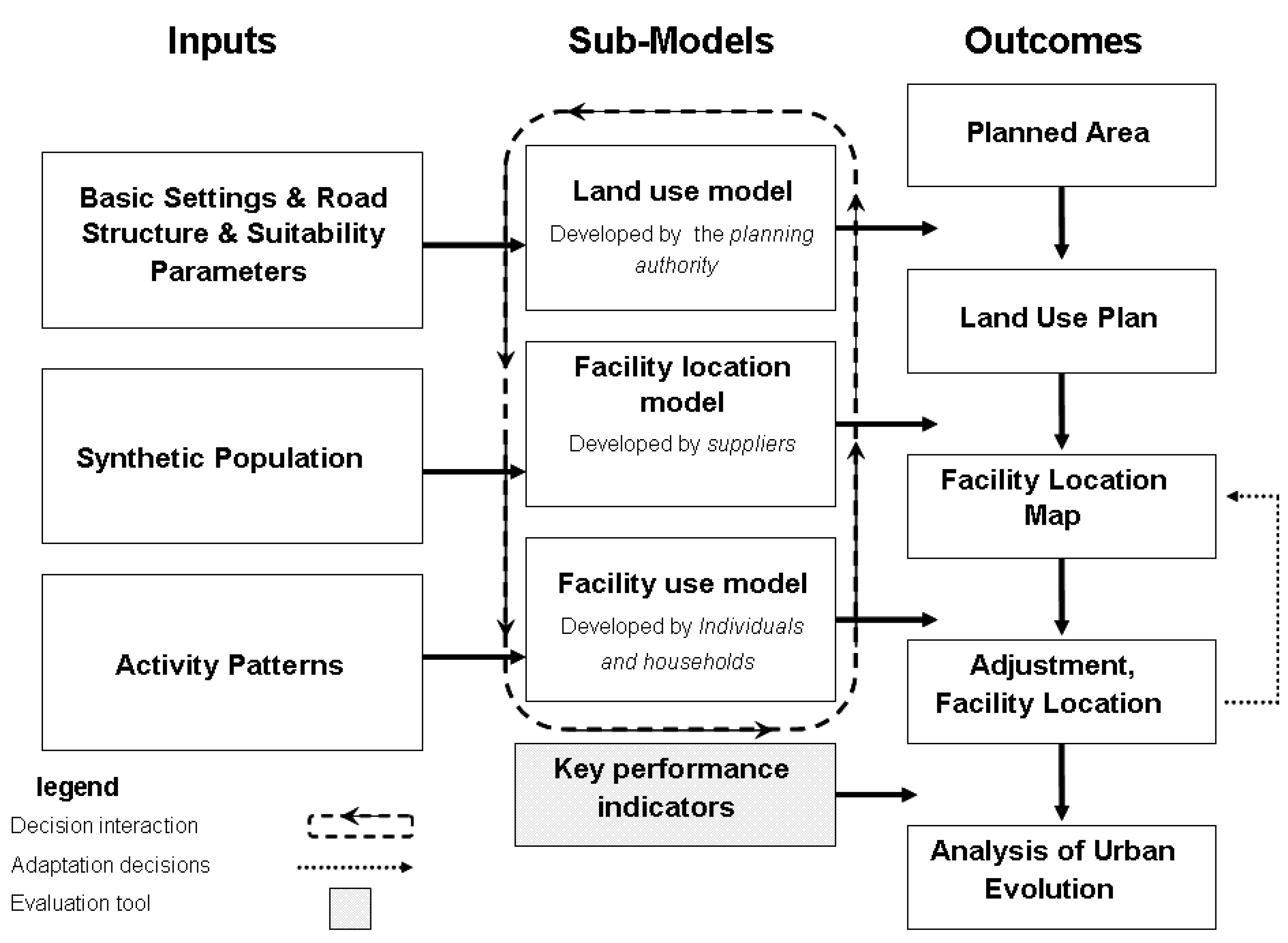
Figure 1 schematically represents the system. It should be emphasized from the start that the model is not a cellular automata model, but can be better viewed as a multi-agent model, describing the behavior of suppliers and consumers/users and a planning support model for allocation land use. The behavior of each agent is modeled separately. The model of consumer behavior is based on empirical data.
Figure 1.
Components of the multi-agent system.
Figure 1.
Components of the multi-agent system.
First, the planning authority decides on the allocation of land use in the form of a zoning plan. This task is supported in the developed system by the Land use model. This stage results in a plan, dividing the study area into zones of different land uses. However, the actual development of facility locations and, therefore, the implementation of a plan, depends on location decisions of firms. These are represented by a second group of actors, named supplier agents, who open and maintain facilities. Their (location) decision making is captured by the Facility location model. Individuals and households, the third group, occupy work places, live in residential cells and use facilities. Their behavior is simulated by the Facility use model.
Obviously, the dynamics of the spatial system are strongly influenced by co-evolving and interactive decisions of these three types of agents. The land use plan constrains the choices of suppliers as it allows only certain developments in certain zones. Similarly, the feasibility and economic viability of particular developments depend on consumer usage patterns and, therefore, on the decisions of households and individuals. Suppliers may respond to these usage patterns by adaptating the size of facilities. In turn, this may lead to changes in usage patterns. These cycles of adaptations continue until convergence is reached.
Each of the models included in the system, the land use model, facility location model and facility use model, requires further operational decisions. We detail them in the next sections.
2.2. The Land-Use Sub-Model
This first model component of the system is responsible for the creation of the land use map. It is based on some input settings that include a definition of the plan area in terms of the number of rows and columns of cells in a regular grid imposed on the area, a definition of the transport network in terms of the main road structure, and the total amount of land that needs to be reserved for each type of land use considered in the model. The development of the land use map is based on a suitability analysis for each cell, in line with common practice in grid-based land-use models (Cromley and Hanink [
29], Riveira and Maseda [
30]). In addition, an allocation algorithm is used to allocate land use to cells in order to maximize overall suitability.
2.2.1. The Suitability Function
The allocation of land use is based on the following suitability function:
where:
G is the exhaustive set of land use types
g, h ⊆ G
i = 1, … , |G| + 2, is an index of land-use types extended with city center and main road
j =1, … , 6, is an index of cut-off-points used to define distance intervals
l is an index of cells
is the suitability of land characteristics of cell l for g
is the weight of distance to land-use/center/road i for g
is a suitability score assigned to the j-th level of distance to i for g
is the suitability of presence of land use h adjacent to g
equals 1, if land use h is adjacent to l and 0 otherwise
is the distance of l from i
is the j-th cut-off-point for distance to i defined for land-use g (ci0 = 0, ci6 = ∞)
Thus, the suitability of a cell l for a particular land-use g is assumed to depend on three factors: accessibility, adjacency and land characteristics. Accessibility is measured with respect to main roads, to the city center and to specific land use categories, h, measured as the minimum distance across all other cells in the plan area that contain land-use h. Adjacency (land use in neighborhood cells) refers to any direct negative or positive effect a particular kind of land use may have on another adjacent land-use (for example, caused by noise, traffic load, decrease of visibility, etc.). It thus refers to the four direct neighboring cells and the four diagonal cells of any particular cell. Finally, land characteristics involve, for example, slope and soil. However, in the current study, this set of factors is not considered.
2.2.2. The Allocation Algorithm
The allocation algorithm assumes as given the total number of cells,
Xg, that need to be allocated for each
g ∈
G, a plan area consisting of a grid of cells,
L, and an initial land-use pattern
gl ∈
G+, ∀
l ∈
L. Here
G+ is an extension of set
G to include vacancy denoted as
gl = 0 (interpreted as non-existence of a land use). Only vacant cells are considered as candidates for allocating new land uses. This means that the plan area can be defined as a subset
Lp of study area
L. The objective of the land-use allocation model can be written formally as:
subject to:
where
g(
l) is the allocated or existing land use of
l,
Lpg ⊆
Lp is the set of locations to which land use
g has been allocated, and other symbols are defined as before. Clearly, an algorithm that finds exact solutions for real-sized problems of this type in reasonable computation time does not exist. Therefore, a heuristic method is used that first generates an initial solution and then tries to optimize the solution by means of land-use swap operations.
2.3. Creating a Virtual Population (the Synthetic Population)
As the model deals with planning for a target population, the distribution of facilities should be based on the demands that result from the activity-travel patterns of a specific population. In order to simulate users, the system creates a so-called synthetic population. This means that for each housing cell a population with certain socio-demographic characteristics is generated, such that the aggregation of these characteristics is consistent with aggregate data. As part of this step, workers are also allocated to industrial and commercial cells to identify their job location. This synthesis uses data based on the Israeli population derived from the same time use survey [
31] used to develop the activity-based model.
The methods used to synthesize the population differ for adults and children. For adults, the system generates a population on a location-by-location basis. That is, for each residential location (cell) the system creates as many agents as there are adults in the population at that location. Agents have a number of attributes including work and marital status, age of the oldest person in the household, socio-economic class, gender, etc. In addition to these attributes, the system also assigns a random day of the week to each agent. In the current system, the allocation to work locations is done separately based on a discrete choice model (i.e., a multi-nomial logit model where workers are allocated to work locations as a function of distance, housing type and employment type).
The generation of the synthetic children population is a derivative of the adult population (in fact the females). The age of the youngest child (if any) is considered an attribute of the household of each female. Based on this attribute, the model reconstructs the family situation by drawing from appropriate distributions: the number of children, the exact age of the youngest child and, for each next child in order of increasing age, the difference in age with the younger brother or sister.
2.4. The Facility Location Sub-Model + the Facility Use Sub-Model
Using the created land use map and the synthetic population, the system distributes facilities across the area. This is based on a simulation of behavior, involving two model components. First, the facility-location model is used to simulate the behavior of facility suppliers in terms of their decisions to open outlets of facilities of specific types. Then, in the next stage, the behavior of the third group of actors, individuals and households who use facilities in the planned area, is simulated by the facility use model. The activities and use of facilities create the drivers for facility suppliers to re-evaluate the developed facilities and make adaptation decisions, if any, in terms of closing or re-sizing facilities.
2.4.1. The Facility Location Model
The facility location model determines the number, type and location of facilities as emergent from agents’ decisions. Agents evaluate candidate facility locations in terms of the number of visitors a (new) facility would attract in a given time period (e.g., a day) based on a catchment area analysis. For each facility type
h ∈
H the system implements an agent, which is concerned with developing and maintaining a network of facilities of type
h (where
H is a pre-defined set of facilities covering the major categories of demand). Thus, a supplier agent incorporates methods to conduct market analysis and make location decisions. The catchment area analysis uses as input the land-use map, the spatial distribution of households in the study area, activity frequencies of these households/individuals and a number of parameters for each facility type. The parameters include: the penetration rate in cells, the radius of the primary and secondary catchment areas, the maximally allowed rate of cannibalism incurred by a facility, a road bonus/penalty, the center bonus/penalty, and size of floor space minimally required for a facility to be viable (for an explanation of the parameters, see
Table 1). In addition, the system also uses an estimate of the proportion of visitors of a certain facility that will also visit another facility if both are in the same location (a synergy parameter). (For further information refer to our previous studies [
26] and [
27]).
The result of this stage is a land use map with facilities. However, in this stage, the location decisions of agents are based on limited information about users. Their behavior is approximated in terms of assumptions regarding activity frequencies, normative expenditures, penetration rates, competition strengths, etc. Uncertainty exists concerning the way the demand will actually be allocated across supply locations by individuals. The latter will be revealed by the facility use model, which is described in the next section.
Table 1.
Facility suppliers-parameters for opening outlets.
Table 1.
Facility suppliers-parameters for opening outlets.
| Parameter | Explanation |
|---|
| Penetration rates | The percentage of population present in a cell that will be attracted to the facility |
| Radius of catchment areas | The radius of the area from which the facility will attract visitors |
| Maximum rate of cannibalism | The extent of allowed overlaps in the primary catchment area between facilities of the same type |
| Center bonus/penalty | Extra demand attracted (positive or negative) due to being in a certain distance from center |
| Road bonus/penalty | Extra demand attracted due to being in a certain distance from amain road |
| Space needed per 100 visitors | Floor space size required for each 100 visitors a day |
| Minimum size of floor space required | Minimum outlet size for a viable facility |
2.4.2. The Facility Use Model
Individuals and households (the third group of actors) who conduct their activities in the planned area, given the locations, sizes and types of facilities, determine the actual needed size and feasibility of facilities. In the system, agents schedule and implement their activities on a daily basis, using the facility use model. A modified version of Albatross [
32], a model of activity-scheduling behavior, is used to simulate the generation and implementation of daily activity-travel patterns. The version of the model that is implemented was estimated based on an Israeli national time-use data set of the Israeli Central Bureau of Statistics (CBS) [
31]. The model predicts for a given day and individual a sequence of activity episodes with associated trips on a continuous time scale while taking temporal constraints, some socio-economic variables, day of the week and spatial variables (location and size of facilities) into account. In-home activities are not further differentiated. The model determines the adults’ activities and children activities differently.
Activities of adults: Scheduling decisions determine which activities are conducted where, for how long, when, and, if travel is involved, the transport mode used. Therefore, an activity episode, which is defined as an uninterrupted period of engaging in a certain activity at the same location, can be described as:
where
a ∈
A is the activity type,
ts the start time,
v the duration,
l the location,
h ∈
H the facility type,
tt the travel time and
m the transport mode of episode
i.
In the model, an individual makes location choices for out-of-home activities in the sequence in which they occur in the schedule. The schedule defines for each activity the transport mode used for the trip to the activity location (based on the location of the previous activity) and the travel time (For further information refer to our previous studies [
26,
27]).
Activities of children: In contrast to the above, the model used to schedule the activities of children is not estimated based on activity or time use data. This is not considered a problem, as the purpose of the model is merely to generate school activities, which are relatively easy to predict for the age groups considered. Given the day of the week and age of the child considered, the model predicts whether or not a school activity is to be included in the schedule for a given day and, if the answer is positive, the attributes of the activity is taken into account. The attributes include the school type (elementary school or high school), start time and end time, and transport mode. The times are based on regular school hours. At present, each activity is allocated to the nearest school from home that matches the school type.
As a consequence of this process, after some time of exploiting the facilities by individuals (adults and children) the actual size of demand attracted will be known. Based on that, the supplier agents then re-evaluate the performance of their developed facilities and make adaptation decisions, if any, in terms of closing or re-sizing facilities. Adaptations of facilities will have an impact on spatial choice behavior of individuals. Therefore, after some time, the supplier agents again consider whether adaptations are needed, and so on. These cycles of adaptations are repeated until convergence.
This finalizes the whole process of the development of the built environment. The outcome is a map that includes land uses and facilities which are relevant and adapted to the targeted population. In the next section, we will describe the use of the multi-agent system as a planning tool for the development of a new city of 150,000 people.
3. The Case Study
3.1. The Four Planning Scenarios
The developed case study is in the niche of using the suggested model/system to create, and in a later stage evaluate, various planning scenarios that differ in their essence in terms of the underlying planning concept. This is based on our assumption that differences in planning scenarios will be responsible for the development of distinctive city forms which naturally influence the development and use of facilities and, hence, will create a different city for people to live in. Four extreme scenarios are considered in this case study. Each one of these four deals with distinctive planning concepts/ideologies. The chosen scenarios are not important themselves; they simply serve as a means for understanding the connection between different (distinct) planning ideas and the built environment.
The Green City is a city with “green lungs”. The idea of this scenario is to develop a city which includes a few areas of Nature cells. These green (Nature) pockets should be large enough to offer the city population some significant open areas in the city texture, a place to use for leisure activities. This scenario was included as it deals with the planning dilemma of how to create a “green environment” and reduce the transportation/accessibility “price” of such a city.
The Mixed City is a combination of high density housing within the commercial area (in the CBD). The idea underlying this scenario is that, in order to create a more compact development with an efficient facility distribution and less need for the reliance on transportation, high density housing should be developed in the city core. This scenario deals with the basic planning question of how to create an efficient built environment where the dependence on traveling in the city for conducting every-day activities is decreased.
The Divided City is a city based on two distinguished areas of dwellings: High density housing which includes apartments in buildings and Low density housing that includes detached houses and houses in a row. The assumption is that in the high density areas, in contrast with the areas of low density housing, facilities should be more accessible and people will be less dependent on traveling for conducting activities. The focus of scenario differs. A relevant question is whether it is possible to plan a city which offers an area of a comparably low density but with appropriate facility dispersal. Such a city might be an appropriate alternative for those looking for detached or semi-detached houses in a suburban development.
The Park City involves a distribution of a number of city-level recreation areas in the city. According to this scenario, the city will include a few big parks, instead of one main central city park. This fourth scenario deals with the choice between spreading a limited number of recreation cells in the city versus concentrating it in one big city park. The question behind this version is: can we use the limited number of recreation city cells and spread them in the neighborhoods to create a feeling of a more “Green City”?
3.2. The Settings
The population size and characteristics, the total number of cells, the number of cells in each specific land use, and the main roads structure are the same for all different planning scenarios included in the study. The planning scenarios differ only in the way the suitability-function parameters are specified, which are defined such that they reflect the underlying idea of each planning scenario.
The main roads structure of the planned area in the present study, for all four planning scenarios, consists of a combination of radial and concentric circular roads, which creates a compact city development (as was found in our previous study [
27] and was mentioned earlier). This road structure is illustrated in
Figure 2. In the current application, the following seven land use categories (denoted as
g within the group
G) were distinguished: (i) Housing High density (to be denoted further as Housing
-H); (ii) Housing Low density (to be denoted further as Housing-
L); (iii) Industry High Tech (Industry-
H); (iv) Industry Low Tech ( Industry-
L); (v) Commercial; (vi) Recreation, and (vii) Nature.
The plan area consists of a regular grid of 2,500 cells of 125 × 125 m in size divided as follows: 760 cells for Housing-H, 400 cells for Housing-L, 96 cells for Industry-H, 96 cells for Industry-L, 96 cells for Commercial land use, 80 cells for Recreation and 972 cells for Nature. The CBD is located in the geographical center of the city. The total size of the area and proportional land use requirements are derived from an anticipated population size of 150,000 people and planning standards. The size of a cell was determined such that it is small enough to accurately represent facility locations, and not smaller to avoid excessive computation times.
The number of housing cells is derived from an assumed housing density degree, as explained below. The number of cells for industrial land use is also based on a density standard (number of workers per industry cell), while the total amount is based on the total population (the total number of workers in the residential population). The number of commercial and recreational cells was based on Israeli planning standards as a function of population size. In this application, the total number of households per cell equals 92 for high density housing cells and 39 for low density housing cells. These numbers follow from the assumptions that, on average, a house occupies 210 m2 and 500 m2 in, respectively, high density and low density cells, and households on average have 1.24 adult members. The number of workers (in full-time equivalence) follows the ratio numbers of 2 (High tech industry), 1 (Low tech industry) and 3 (Commercial). The simulation is based on a sample fraction of 10% of the population.
Figure 2.
The main roads structure of the planned area.
Figure 2.
The main roads structure of the planned area.
3.2.1. Setting the Suitability Parameters—Creating the Outline Plan
The suitability parameters for the land use model were set based on two kinds of information: (1) a conjoint study (see Katoshevski and Timmermans [
33]), which measured preferences of individuals for land uses, facilities and relative location, such as preference concerning the dwelling location in relation to different city/neighborhood facilities, and (2) heuristics that planners use to find the spatial arrangements of land-uses that meet planning standards. For each of the planning scenarios the basic setting of suitability-function parameters (see recent work by Katoshevski-Cavari [
27] and
appendix) was changed so that they support the specific planning idea. The major differences in suitability parameters defined differently for each of the four planning scenarios are summarized in
Table 2 and are explained in later paragraphs.
Appendix 1 gives all suitability parameters.
1. The Green City. In this scenario, the parameters for the Housing and Nature cells were set so that they will support the desired distribution of Nature cells in the city. A clear preference was determined for the Housing cell to be close to the Nature cells, and for Nature cells to neighbor other Nature cells so that Nature polygon(s) will be created.
2. The Mixed City. As the idea of this scenario is to “push” Housing-H cells into the central part of the city (the CBD), the parameters in this scenario were set so that a high score is given for the Housing-H cells to be close to Commercial cells, and vice versa.
3. The Divided City. In order to create a clear separation between the Housing-H cells and the Housing-L cells, the suitability parameters were determined so that a strong connection is defined for each Housing cell to be close to its same kind of Housing, and low weight score (low preference) for being close to the other Housing kind.
4. The Park City. In this case the suitability parameters are showing preferences for short distances between the Housing and the Recreation cells. This is determined for all dimensions included: the cut-off points, suitability scores and weight scores, and adjacency scores.
Based on the described suitability parameter settings of each planning scenario, the system allocates the required land uses to cells. This results in a land use pattern which represents an outline plan. This plan is the basis for generating the synthetic population and facility networks, as explained earlier.
Table 2.
The four scenarios—The parameter settings for developing land use.
Table 2.
The four scenarios—The parameter settings for developing land use.
| Dimensions | City scenarios |
|---|
| Green City | Mixed City | Divided City | Park City |
|---|
| Cut-off points | Housing to Nature: 200 m, 400, 600, 800 | Housing-
H to Commercial: 200 m , 400, 600, 800 Commercial to Housing-H: 400 m, 600, 800 | Housing-to Housing (all kinds): 100 m, 200, 300, 400, 500 | Housing to Recreation 200 m, 400, 600, 800 Recreation to Housing: 100 m, 200, 300, 400 |
| Suitability scores | A monotonically decreasing function of distance regarding all land uses | Housing
-H to Commercial: A monotonically decreasing function of distanceCommercial to Housing-H: decreasing until 800 m and zero thereafter | A decreasing function of distance, and zero from 500 m and on | A monotonically decreasing function of distance |
| Weight | 5 | 5 | Housing to its same kind: 5; to the other kind: 2 | 5 |
| Adjacency scores | Housing to Nature: 5
Nature to Housing-
H: 5
Nature-Nature: 10 | Housing-
H to Commercial and Commercial to Housing-H: score of 5 | Housing-
H to Housing-H and Housing-L to Housing-L: score of 10 | Housing (both kinds) to Recreation: 10. Recreation to Housing-
H: score of 10 |
3.2.2. The Facilities
As explained in the theoretical part, a facility location model is used to simulate the behavior of suppliers of facilities. Nine classes of facilities were distinguished in the system corresponding to the main facilities a city of 150,000 people should provide.
Table 3 gives an overview of these facilities on main class and subclass levels (note that location decisions by supplier agents and demand allocation decisions by individuals are made on the subclass level).
Table 4 represents a further operational decision made in the simulation that concerns the question as to which facilities are allowed in the different land use cells. As can be seen in the table, most facilities can be located in cells of three land use types: Housing
-H, Housing
-L and Commerce.
The parameters of the facility location model (which were defined in
Table 1) were set the same for the different planning scenarios as all are based on Israeli planning norms and standards. This setting will be shortly described.
Penetration rates for primary catchment areas were set between 0.4–0.8, with the lower levels given to the daily shopping-city level, medical-city level, theatre, pool and a large sport hall, and the higher levels to non-daily shopping neighborhood level and neighborhood parks. For secondary catchment areas, the penetration rates were set between 0.1–0.4, with the lower values for daily and non-daily shopping at the neighborhood level, activity center, post offices, banks, synagogue and small sports hall, and higher levels for hospitals and city parks. For the primary as well as secondary catchment areas, in general, lower penetration rates were indicated for the neighborhood facilities. The lower penetration rates in the secondary catchment area compared with the primary catchment area reflects the typical distance decay effects.
Table 3.
Facility classification (classes and subclasses).
Table 3.
Facility classification (classes and subclasses).
| Main class | Subclass |
|---|
| Daily shopping | Neighborhood level |
| City level |
| Non daily shopping | Neighborhood level |
| City level |
| Schools S | Kindergarten |
| Elementary school |
| Schools H | High school |
| Medical | Neighborhood level |
| City level |
| Hospital |
| Leisure | Restaurant |
| Activity centre |
| Theatre |
| Services | Post |
| Bank |
| Library |
| Synagogue |
| Sport | Pool |
| Sport hall small |
| Sport hall big |
| Parks | Neighborhood |
| City |
Table 4.
Facility location by land use.
Table 4.
Facility location by land use.
| Facility | Land use |
|---|
| Housing High | Housing Low | Industry L | Industry H | Comm | Green | Nature |
|---|
| Daily shopping | + | + | | | + | | |
| Non-daily shopping | +only neighborhood level | +only neighborhood level | | | + | | |
| School (kinderg + elementary) | + | + | | | + | | |
| School high | + | + | | | + | | |
| Medical | + | + | | | + | | |
| Leisure | + | + | | | + | | |
| Services | + | + | | | + | | |
| Sports | + | + | | | + | | |
| Park | +only neighborhood level | +only neighborhood level | | | | + | |
In terms of the radius of catchment area, a small catchment area was chosen for all neighborhood facilities. This is meant to keep these facilities at a short distance from housing and spread them across the city, initially. The primary catchment area has a radius of 500 m for neighborhood facilities. High school is the only neighborhood facility with a larger catchment radius (750 m) as the required population size for opening a high school facility is usually larger than a normal neighborhood population. For the city level, the radius varies between 1,550 m for the non-daily shopping facilities and 2,350 m for hospital and city Park (which are each a single facility in the city).
The maximally allowed rate of cannibalism was set to percentages between 30% and 70%. Usually the numbers were set between 30% and 45% for neighborhood facilities, and assumed to be higher-70%—for city-level facilities. This compensates a lower penetration rate in the catchment area of the facilities which lead to a relatively small number of visitors from the neighborhood.
The center bonus/penalty was chosen such as to elucidate that the neighborhood facilities are staying within the neighborhood area although a penalty was given for main neighborhood facilities when located in the central area of the city. The penalty value ranges between −1 and −20. In contrast, facilities expected to be located in the central part of the city were given positive bonus values in order to “pull” the facilities to the center. These values range between 1 and 20. The road bonus/penalty parameters had a very limited use in this application and included only penalty scores for high schools and city-level daily and non-daily shopping for being close to roads.
Finally, the parameter “space needed per 100 visitors” and “minimum size of floor space required for the facility to be viable”, were set dependent on the kind of the facility, its level (neighborhood or city) and the relevant maximum size. We emphasize that the choice of parameter settings, which determine how supply agents perform catchment area analyses for determining facility locations, is not critical for the behavior of the system, since supplier agents are able to adapt their initial decisions based on actual (simulated) behavior of households and individuals.
4. The Results
4.1. The Four Land Use Maps
The land use maps, which were developed by the system based on the described four planning scenarios, are portrayed in
Figure 3,
Figure 4,
Figure 5 and
Figure 6 and will be described now.
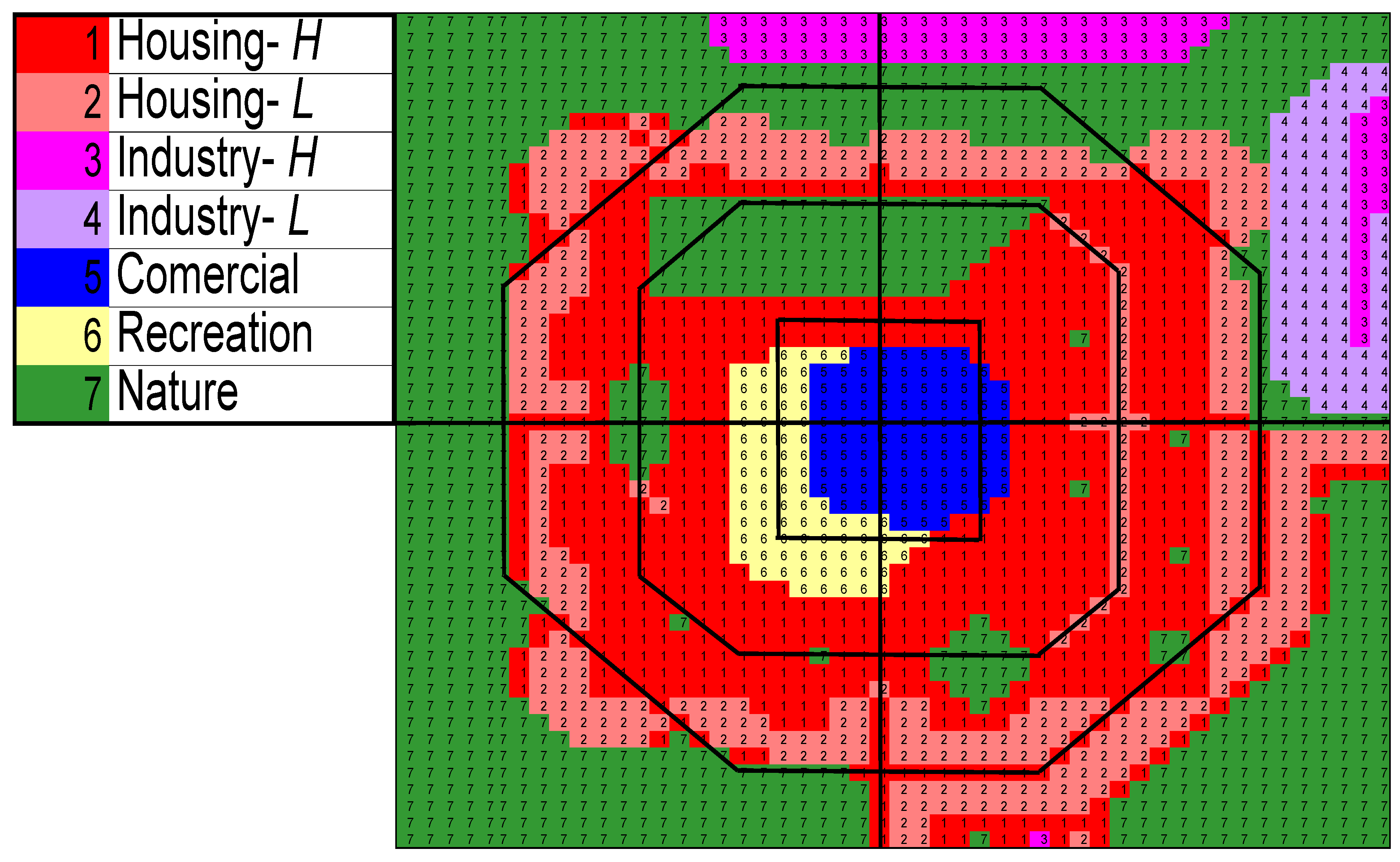
1.
The Green City. The land use pattern that emerges for this city is portrayed in
Figure 3. In this plan, the city center primarily has commercial land use and adjacent to this a big recreation area. Industrial areas appear in the periphery of the city. Houses are developed around the central part of the city where, in general, Housing
-H cells are closer to the center, and Housing
-L cells are developed at a greater distance from the center, towards the outer part of the city. A special feature of this city concerns the pockets of green area (one big area and some small ones), spread in the built environment.
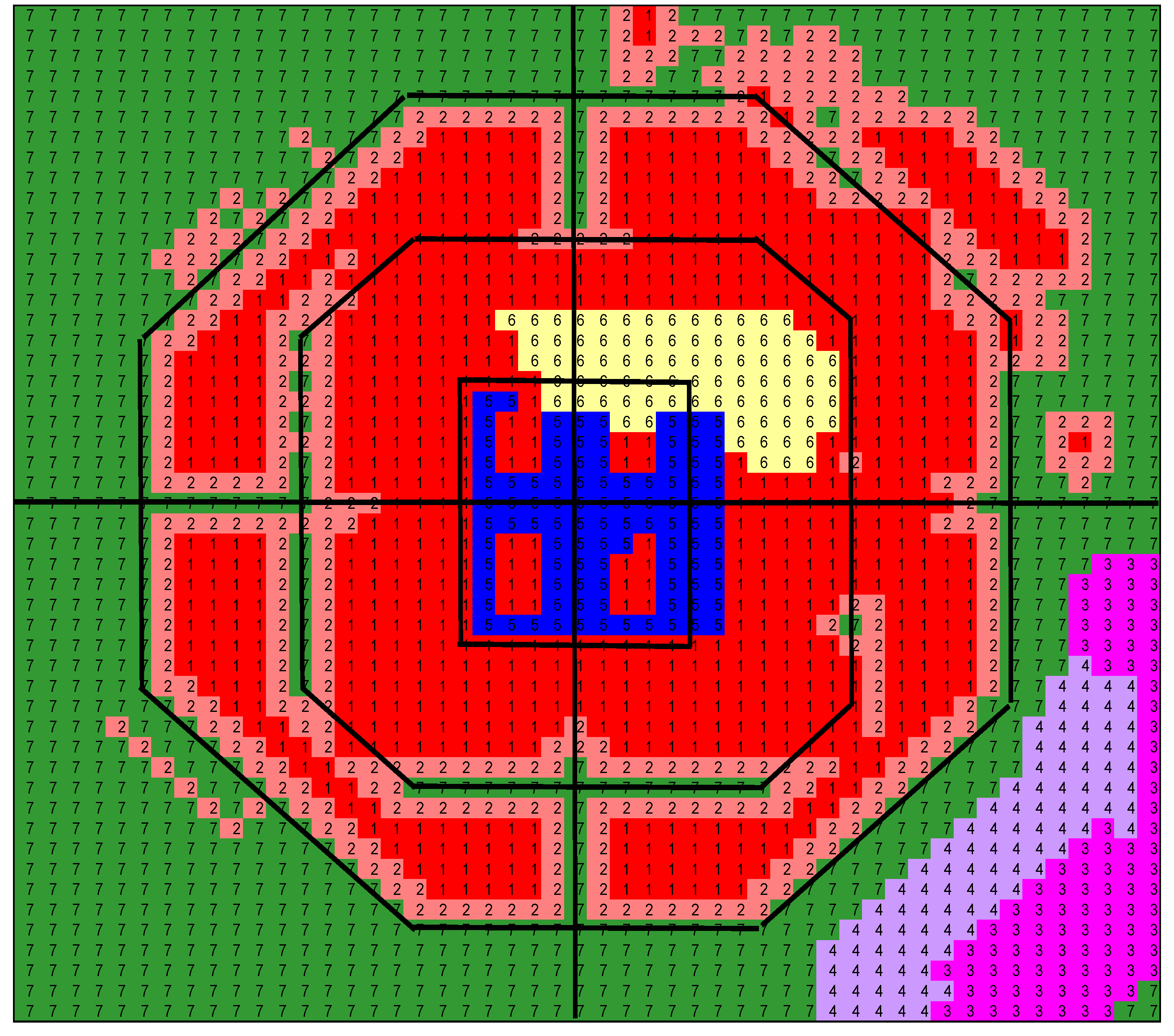
2.
The Mixed City. The land use pattern that emerges for this city is portrayed in
Figure 4. In this plan, the city center has a mix of commercial cells and Housing
-H cells. Interesting is that this denser and compact area of the central part of the city stands in contrast to the structure developed in the outer part where some nature cells penetrate into the built area of the city and Housing
-L is developed around these cells. Similar to the previous plan, the city includes one main city central park which is developed adjacent to the CBD and an industrial area that is developed in the outer part with some distance from dwellings.
Figure 3.
The Green City—Land-use colors and numbers are shown in the legend. The dimensions of each cell are 125 m × 125 m.
Figure 3.
The Green City—Land-use colors and numbers are shown in the legend. The dimensions of each cell are 125 m × 125 m.
Figure 4.
The Mixed City—Land-use colors and cell size are same as in
Figure 3.
Figure 4.
The Mixed City—Land-use colors and cell size are same as in
Figure 3.
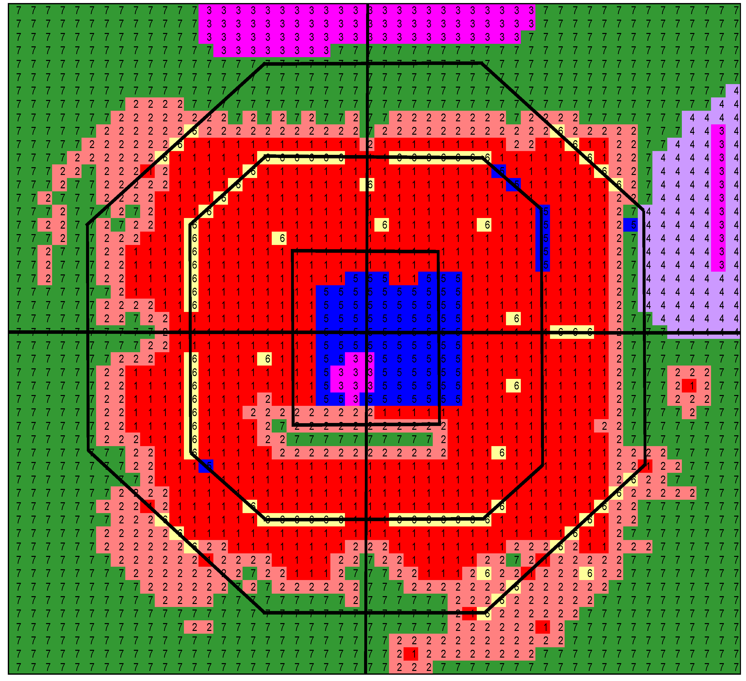
3.
The Divided City. In this plan (
Figure 5), the city center again includes a concentration of Commercial cells. Adjacent is a large Recreation site. Industrial areas appear in the periphery of the area. However, differently from the other versions, the dwelling cells are developed in two areas: an area of Housing
-H is developed around the central part of the city, with no penetration of Nature cells, creating a dense area, and an area of Housing
-L is developed in the outer area of the city, creating one big site which is surrounded by Nature cells.
4.
The Park City. In this plan (
Figure 6), in contrast to all three other plans, the city does not have a large, main central park. Rather, park cells are spread across the city creating many, different sized recreation parks. In this plan as in all previous ones, the central part of the city mainly consists of Commercial cells. However, in this scenario the CBD includes also some Industry
H cells. Another main difference of this scenario is the development of Commercial cells in other parts of the city in addition to the CBD. All other Industrial cells are developed in two sites in the outer part of the city. In that part of the city, the development of Housing is not dense and it is combined with Nature cells.
Figure 5.
The Divided City—Land-use colors and cell size are same as in
Figure 3.
Figure 5.
The Divided City—Land-use colors and cell size are same as in
Figure 3.
Figure 6.
The Park City—Land-use colors and cell size are same as in
Figure 3.
Figure 6.
The Park City—Land-use colors and cell size are same as in
Figure 3.
4.2. Facility Location Patterns
These different cities, in terms of land use patterns, provide distinct platforms for suppliers to locate their facilities, and for individuals/ households to conduct their activities. For each one of the city plans the supplier agents developed facility networks. This process includes several cycles of adaptation, as explained in the theoretical part of the paper. The result of this process after convergence is a city with a particular spatial distribution of facilities. For each city version the model creates nine facility maps (one for each facility class). These maps present the facilities distribution in the city.
Figure 7 is an example of such a map. This presented map describes the distribution of kindergartens and elementary schools in the Park City. As can be seen, kindergartens and elementary schools are not spread homogenously in all city areas, they have higher number-density in the inner areas of the city than on the outskirts. The essence of the facility distribution, for each planning scenario, is presented in the following paragraphs.
1. The Green City. The daily and non-daily shopping facilities and school facilities are spread all over the city, with daily shopping showing a slightly more distributed pattern than non-daily shopping. High schools display a more spread pattern than elementary schools. Medical, services, leisure, sports and park facilities are all spread in the city with very limited emphasis on the city center.
2. The Mixed-City. Daily and non-daily shopping facilities are all spread in the city. The daily shopping facilities show better coverage. The school facilities and medical facilities also are developed in all parts of the city. The leisure facilities and services facilities are also spread in the city. The pattern places a very limited emphasis on the center. Sports and park facilities also are spread in the city.
3. The Divided City. Most facilities show a more scattered pattern in the Housing-H areas than in the Housing-L areas. Some facilities are completely absent in the Housing-L cells (non-daily shopping and elementary schools facilities) and some appear in the Housing-L areas but in limited numbers (for example the daily shopping facilities). The only exceptions are medical, services and sports facilities. In addition, in most cases in the Housing-L area, facilities are not plotted evenly but rather are attracted towards the central part of the city that is at a distance from the city edges, creating an inequality of the spreading pattern of the facility in this part of the city.
4. The Parks City. Daily neighborhood-level shopping facilities are spread all over the city, whereas daily city-level shopping facilities tend to be developed more towards the center. Non-daily shopping facilities show the same pattern, but all is more towards the central part of the city supplying fewer facilities to the outer part of the city. The school, medical, services, sports and parks facilities are also spread across the city. However, as mentioned above, kindergartens and elementary schools are not spread homogenously in all city areas, they have higher number-density in the inner areas of the city than on the outskirts. Hence, although the averaged distance to those facilities seems reasonable, those living on the outskirts of the city have larger travel distances than those living in the inner areas. The leisure facilities are also spread out but show, nevertheless, clear concentration in the center.
Figure 7.
The Park City—including school facilities (land-use colors and cell size are same as in
Figure 3). 1: kindergarten; 2: elementary schools.
Figure 7.
The Park City—including school facilities (land-use colors and cell size are same as in
Figure 3). 1: kindergarten; 2: elementary schools.
5. Effects of Urban Form on Performance Indicators
The resulting spatial configuration of land and facilities can be compared in the model by using a series of key performance indicators. This feature is important for the comparison between the different scenarios and for drawing planning conclusions. In this section, we will describe the different indicators used in this case study and the results of a comparison between the four created alternatives, based on these indicators. Two of the performance indicators used in the study are transportation-sustainability oriented, in line with the transportation-accessibility planning issues relevant nowadays.
1.
Accessibility reflects the ease of access of facilities, which is the inverse of the distance needed to reach different facilities from home locations. It is commonly assumed that better accessibility is a positive indicator of sustainable development. For each facility type (at the subclass level) a number of accessibility measures are calculated. These include: the average distance to the nearest facility across housing cells (home locations), the average distance to the second nearest facility across housing cells and the average number of facilities (of that type) within a distance of 750, 1,250 and 2,250 m across housing cells. In calculating these averages, the size of the population in a housing cell is used as a weight. The average distances to the first and second facility are portrayed in
Table 5The results of the accessibility analysis of the city shows that the Park City creates in general a more accessible pattern for using the first nearest facility, and the Green City creates the best pattern in terms of accessibility of the second nearest facility. A good accessibility regarding the second nearest facility indicates that consumers have within a short distance multiple facilities available and, hence, have the advantage to choose between alternative destinations. Hence, the Green City scenario suggests a relatively good choice/opportunity. When examining the various facility levels from the general city one to the classes and sub-class levels, the mean accessibility scores regarding the first nearest facility in the different city scenarios are not consistent in monotonic behavior: The Mixed City seems to offer the best access in terms of services, sports and parks facilities, the Divided City offers an overall better accessibility of elementary schools and medical services, and the Park City offers better accessibility concerning daily and non-daily shopping, high schools, leisure and sports facilities. However, these results concern an overall city calculation. The underlying patterns have unique features in many cases. For example, in the Divided City, the very convenient distribution of elementary schools in the Housing-H area compensates the less attractive distribution in the Housing-L area and hence shifts the overall city average.
2. Analysis
of transport demand (mobility) in the system is based on the trips resulting from a one day run of the facility use model. For each activity type (at subclass level) the model determines the distance traveled (a straight line distance in meters) for each trip conducted for the activity type. The results represent the overall average distance traveled for each facility type and is shown in
Table 5.
According to our calculations, in the Park City the number of tours and the total travel distance are lowest. Disaggregated by facility class, the results show that Park City generates the shortest mean distance traveled for the shopping facilities (together with the Divided City concerning the daily-shopping), high school, leisure, services and park facilities. The Mixed City creates the shorter mean distance for the elementary school facilities and sports facilities. The Divided City, in addition to daily shopping, also results in a shorter mean travel distance to the medical facilities.
3.
Viability, the third set of indicators, refers to the economic performance of the facilities. For each facility type (at the subclass level), the model determines a few measures for each outlet of that type such as the number of outlets, the ratio (between the actual size and the minimum size of the outlets) and the cluster size (the total number of facilities across types located at the same location). The results concerning these aspects are also portrayed in
Table 5.
Table 5.
Effects of urban forms on performance indicators.
Table 5.
Effects of urban forms on performance indicators.
| Facility | Accessibility | Mobility | Viability |
|---|
| Distance to first nearest (mean in meters) | Distance to second nearest (mean in meters) | Total distance traveled (mean in meters) | Number of outlets | Ratio (mean)* | Cluster size (mean) |
|---|
| The Green City |
| Daily shopping | 640 | 1,224 | 1,137 | 14 | 3.15 | 2.64 |
| Non-daily shopping | 1,127 | - | 1,212 | 12 | 3.57 | 1 |
| Elementary school | 583 | 1,076 | 548 | 25 | 2.52 | 2.08 |
| High school | 593 | 1,178 | 867 | 10 | 4.6 | 1.3 |
| Medical | 645 | 943 | 1,175 | 23 | 2.42 | 1.74 |
| Leisure | 822 | - | 1,264 | 28 | 2.86 | 2.36 |
| Services | 410 | 784 | 1,117 | 90 | 4.65 | 2.29 |
| Sports | 1,111 | - | 1,405 | 18 | 4.05 | 2.56 |
| Parks | 646 | - | 1,044 | 22 | 8.26 | 2.82 |
| The Mixed City |
| Daily shopping | 601 | 1,073 | 1,100 | 16 | 2.8 | 3.06 |
| Non-daily shopping | 1,096 | - | 1,155 | 12 | 3.68 | 1.58 |
| Elementary school | 493 | 907 | 485 | 26 | 2.32 | 2.85 |
| High school | 588 | 1,093 | 902 | 11 | 4.07 | 1.09 |
| Medical | 653 | - | 1,277 | 20 | 2.7 | 2.7 |
| Leisure | 681 | 1,127 | 1,189 | 33 | 2.58 | 2.58 |
| Services | 410 | 805 | 1,108 | 79 | 5.37 | 3.13 |
| Sports | 876 | 1,430 | 1,238 | 21 | 3.17 | 2.71 |
| Parks | 643 | 673 | 1,020 | 22 | 8.1 | 2.05 |
| Sports | 880 | 1,422 | 1,278 | 20 | 3.38 | 1.8 |
| Parks | 678 | - | 1,046 | 20 | 8.74 | 2.1 |
| The Divided City |
| Daily shopping | 599 | 1,045 | 1,078 | 16 | 2.83 | 1.56 |
| Non-daily shopping | 1,110 | - | 1,171 | 12 | 3.6 | 2.08 |
| Elementary school | 522 | 858 | 509 | 28 | 2.18 | 2.93 |
| High school | 624 | 1,240 | 888 | 10 | 4.66 | 1.1 |
| Medical | 620 | - | 1,137 | 21 | 2.62 | 1.62 |
| Leisure | 717 | 1,143 | 1,187 | 30 | 2.77 | 1.8 |
| Services | 434 | 852 | 1,102 | 73 | 5.76 | 2.29 |
| Sports | 880 | 1,422 | 1,278 | 20 | 3.38 | 1.8 |
| Parks | 678 | - | 1,046 | 20 | 8.74 | 2.1 |
| The Park City |
| Daily shopping | 586 | 1,052 | 1,079 | 15 | 2.87 | 2.07 |
| Non-daily shopping | 1,042 | - | 1,112 | 13 | 3.29 | 1.46 |
| Elementary school | 537 | - | 527 | 21 | 2.65 | 1.76 |
| High school | 575 | 1,070 | 836 | 11 | 4.23 | 1.09 |
| Medical | 623 | 953 | 1,202 | 20 | 2.71 | 2.3 |
| Leisure | 676 | 1,029 | 1,164 | 77 | 1.1 | 1.44 |
| Services | 417 | 780 | 1,067 | 81 | 5.08 | 1.33 |
| Sports | 876 | 1,359 | 1,248 | 20 | 3.44 | 1.8 |
| Parks | 650 | - | 1,019 | 23 | 7.63 | 1.61 |
The results for the total number of outlets are 242 outlets for the Green City, 240 outlets for the Mixed City, 230 outlets for the Divided City, and 281 outlets for the Park City, indicating that the Park City has the largest facility network. Looking at the level of the different facilities, as indicated in
Table 5, the Figures do not show a clear direction of any of the city forms. The results concerning the ratio between the actual size and the minimum size of the outlet are 4.16 for the Green City, 4.17 for the Mixed City, 4.34 for the Divided City and 3.5 for the Park City. This measure shows that, in general, the Divided City has the best economic performance. Finally, the Table shows the mean cluster size. The results are as follows: a cluster size of 2.21 in the Green City, 2.67 in the Mixed City, 2.07, Divided City and 1.76 in the Park City. Thus, the Mixed City has the advantages of somewhat increased spatial agglomeration and efficient use of space. Again, in terms of these two indicators, the distributions of facilities do not show a clear tendency for any of the city forms overall (as can be seen in
Table 5).
6. Discussion and Conclusions
The study reported here had two objectives. First, we were interested in examining the effects of different planning ideas/scenarios on the development of a (sustainable) new city: how do different planning ideas influence the development and performance of a city? Using a theoretical approach, we considered several scenarios to examine the relationships between planning concepts, road structure and a sustainable (accessible) built environment. The second goal of this study was to illustrate the application of the developed multi-agent model as a tool for planners and decision makers to develop and evaluate planning alternatives. For these two purposes, different outline-plans and facility networks were created and evaluated in terms of several externalities.
The case study included a development of a hypothetical city planned for 150,000 people, based on behavior of suppliers and consumers, the targeted population preferences and expert (planners) knowledge. Four alternatives were created based on four distinct planning scenarios. The outcome for each scenario is a city with land uses and facilities presented as a master plan.
Although all scenarios had this common base, the four emerged plans are different in their land use and facility distribution. Thus, each plan creates a special city configuration, which differs in the environment they offer for the dwellers. In the land use maps, clear differences are obvious. The Green City offers the dwellers a few pockets of nature spread across the city. The Mixed City plan created an area of mixed use in the central part of the city allowing people to live in the CBD. However, this efficient land use mixture does not penetrate into the other parts of the city. The Divided City, which is probably the most exceptional scenario, resulted in the development of two distinct areas. It seems that the compactness of the city is kept only for the Housing-H cells which are developed around the center. The Housing-L cells are developed in a different area. Finally, the Park City, offers a number of city level parks spread throughout the city instead of one big park.
These created cities are different in their basic underlying planning concept and, as shown in the developed land uses, also include unique facility distributions. In terms of performance indicators, the results did not clearly identify the most accessible city, the most efficient city (mobility) or the most economically viable (viability) city plan. However, the Park-City shows slightly higher efficiency in terms of mobility aspects and more accessible facilities than the other cities. Hence we claim that from the transportation/accessibility point of view, this is the most sustainable city form in the current study. This sustainability is probably due to the fact that city parks are spread out instead of concentrated in one park area, which enables facilities to be distributed along a more accessible configuration. In addition to the advantage of the distribution of recreation cells in the city, this scenario also creates a more efficient facility distribution. The Park-City scenario, which was included in the study in order to understand the transportation/accessibility “price” of including Nature cells in the city, created the best pattern in terms of accessibility to the second nearest facility.
The results lead us to conclude that the road structure plays an important role in keeping the city compact and creating an efficient facility distribution i.e. a sustainable compact built environment can be kept while implementing different planning ideas. Hence, different planning ideas, some of which (as expected) do not seem to support city compactness (the Divided-City, or the Green-City), can be introduced in urban planning with only a limited expense of “loosing” efficiency of the facility distribution. For example, the Divided-City scenario resulted in an outer area of Housing-L cells, which are responsible for creating a more spread distribution of land uses. Although the facilities were not distributed evenly, it did not result in a much loss of efficiency. This conclusion concerning the role of the road structure is important for planners and decision makers when planning a new area, enabling them to base their planning on different ideas, yet still keep an efficient city facility distribution.
The current illustration only considered central cities. Planning literature not only discusses compact cities and multiple land uses, but also the impact of peripheral development. To examine the impact of centralized versus multi-nuclei development, additional city forms should be designed and then a similar process of model application could be developed. This we will do in future research.
As for the second purpose of the study, the relevancy of this model/system as a planning tool, we can conclude that the multi-agent model can be used as a tool for planners. It demonstrated the ability to create a master plan (land use and facilities) that is relevant for a target population, taking into account peoples' preferences and planning norms. The suggested tool uses a systematic planning process for the creation of a plan. In addition, it takes into account peoples’ preferences, aspects that are often neglected in the common planning process. Hence, this system suggests an alternative planning tool for planners to use in the first creative phases of a planning process. In addition, the decision support system can be used for evaluating different planning options (created by the system or created separately) using the performance indicators, which can be defined on the basis of the relevant planning agenda.
It should be noted, however, that although we demonstrate the ability and relevancy of this system to create a master plan, we cannot ignore the fact that the method is relatively complex. Hence, realistically, this and similar tools will be used mainly in the planning of high priority projects.


