
Electric Vehicle Routing Problem with States of Charging Stations

Department of Industrial Management Engineering, Hanbat National University, Daejeon 34158, Republic of Korea
Sustainability 2024, 16(8), 3439; https://doi.org/10.3390/su16083439
Submission received: 25 March 2024
/
Revised: 14 April 2024
/
Accepted: 16 April 2024
/
Published: 19 April 2024
(This article belongs to the Topic Electric Vehicles Energy Management, 2nd Volume)
Abstract
:This paper proposes an electric vehicle routing problem, considers the states of charging stations and suggests solution strategies. The charging of electric vehicles is a main issue in the field of electric vehicle routing. There are many studies that find the locations of charging stations, recharging functions for the batteries of vehicles, and so on. However, the state of charging stations significantly affects the routes of electric vehicles, which is not much explored. The states may include open or closed charging stations, occupied or empty charging slots, and so on. This paper investigates how the states of charging stations are estimated and how routing strategies are determined. We formulate a mixed integer programming model and suggest how to solve the problem with an exact method. Numerical examples provide the optimal routing strategies of electric vehicles for the changing environments regarding the states of charging stations.
1. Introduction
The fast growth of air pollution and global climate change has driven the consideration of sustainability in various sectors including energy, manufacturing, logistics, and so on. Countries are forced to reduce the use of fossil fuel as it is the main cause of global warming. Transportation has accounted for more than 23% of greenhouse gas emissions causing air pollution (Xiao et al., 2021 [1]). Accordingly, transportation has been changed to encourage the use of electric vehicles rather than internal combustion vehicles. The study of the vehicle routing problem has been extended to the study of the electric vehicle routing problem. The electric vehicle routing problem has become an important issue in the field of sustainability.
Many studies have been conducted for the electric vehicle routing problem. Compared to the conventional vehicle routing problem, the electric vehicle routing problem has additional issues, while both problems aim to find the optimal route from the alternatives. The issues of the electric vehicle routing problem include finding the optimal location of charging stations, estimating the recharging functions of the battery and energy consumption, and so on. Most studies are related to charging the battery of electric vehicles. Without the charging issue, the problem is the same as the conventional vehicle routing problem. The issue with location is to find the optimal locations of charging stations, minimizing the total travel costs. With vehicle routing, this problem becomes the location routing problem. For the charging function, the problem is to find the change or pattern of charging level by time. The function is assumed as a linear or nonlinear function. Since the charging time is long, there are some studies on partial charging instead of full charging. Research questions include where the charging stations are in place and how to charge the battery.
On the other hand, there is a lack of studies into the states of charging stations. When an electric vehicle arrives at a charging station and all charging slots are occupied, the electric vehicle may have to wait for a long time. If the charging station is closed, the electric vehicle should go to another charging station. The state of the charging station can be defined by its availability. If the charging station is not available when the vehicle arrives, this situation significantly affects its route. Thus, this paper considers the states of charging stations for the electric vehicle routing problem. Each charging station has its own state. The states for charging stations may have distributions or patterns. Once the patterns of the states are found, one can find the optimal location routes of electric vehicles.
One of the concerns for the electric vehicle routing problem is that the charging time is too long, rather than the issue of using fossil fuels. Due to their long charging time, vehicles occupy the charging slots for an extended period, so there may be lack of available slots. If the stations are crowded, the availability does matter. For example, assuming a vehicle arrives at a charging station and all charging slots are occupied, if the earliest available slot is in thirty minutes, the vehicle has to wait at least thirty minutes. The states of the charging station are not deterministic, but random or stochastic. Each station has a different uncertainty such as open/closed, occupied/empty, normal/out of order, and so on. These uncertainties present the availability of the charging station. Assuming there are multiple deliveries, each vehicle travels twice in a day, and needs to recharge one time either in the first time period or the second time period. If a vehicle’s battery is recharged in the first time period, the vehicle can travel without recharge in the second time period. On the other hand, if the vehicle wants to recharge in the second time period, the vehicle can travel without recharging in the first time period. In this case, the vehicle has to decide the time period to recharge to minimize the total travel costs in a day. Depending on the states of charging stations, we can decide when to recharge the battery for each vehicle. Thus, the patterns for the states of charging stations can be used as input parameters in the electric vehicle routing problem.
The contributions of this paper are as follows: This paper suggests an electric vehicle routing problem with states of charging stations and an optimization model. Depending on the states of charging stations, the optimal routes may be different. We also propose the strategy to achieve the optimal routing plans for vehicles. Vehicles must decide when and where to go at the next time period to minimize the total travel costs. Lastly, this paper provides some numerical experiments to show the viability of the proposed solution approach.
This paper presents the literature about this issue in Section 2. Section 3 describes the problem and a mathematical model for the electric vehicle routing problem. Section 4 proposes solution methods for the electric vehicle routing problem with the states of charging stations. Numerical examples and results are presented in Section 5. Finally, this paper summarizes the paper and discusses future work.
2. Literature Review
The electric vehicle routing problem has become an interesting issue in a variety of different fields such as transportation, energy, sustainability, and so on. Researchers have focused on charging-related issues or solution approaches. This section presents the related works for the electric vehicle routing problem rather than the conventional vehicle routing problem.
Various problems for the electric vehicle routing problem have been considered. Chakraborty et al. (2021, [2]) have dealt with the electric vehicle routing problem to find optimal charging schedules and routes. Schneider et al. (2015, [3]) have introduced time window constraints in the electric vehicle routing problem. Keskin et al. (2019, [4]) have considered the electric vehicle routing problem with time windows and explored the queues at charging stations. Hiermann et al. (2016, [5]) have also explored the electric vehicle routing problem with different vehicle sizes. Charging the vehicle has also been explored. Montoya et al. (2017, [6]) assumed a nonlinear function for the charging rate and suggested proper charging behavior. Froger et al. (2019, [7]) used a nonlinear function and proposed arc-based and path-based tracking of the time approach rather than a node-based model to avoid replicating the charging station nodes. If vehicles are fully charged during the travel, the total traveling time will be significantly increased. Instead of full charging, partial charging has been proposed in many studies. Bac and Erdem (2021, [8]) proposed the electric vehicle routing problem with multiple depots and heterogeneous fleets. Basso et al. (2021, [9]) also considered partial charging. In their research, the problem has included uncertainties such as road condition or energy consumption. Hybrid electric vehicles have been considered. In their research, Kasani et al. (2021, [10]) investigated electric vehicles and hybrid electric vehicle routing and scheduling problems in the private and public sectors. Ma et al. (2021, [11]) suggested the shared autonomous electric vehicle routing problem with battery swapping and proposed a speed optimization model on the travel arc. Pelletier et al. (2019, [12]) explored the uncertainty of energy consumption during a delivery tour. Al-dal’ain and Celebi (2021, [13]) investigated the problem of the vehicle compositions of electric and conventional vehicles to minimize total operational costs in urban areas. Brady and O’Mahony (2016, [14]) tried to find the patterns of travel of the vehicle and charging behavior. They used a dataset of vehicles traveling to resolve uncertainty.
For the modeling of the electric vehicle routing problem, studies have adopted optimization models. Mixed integer programming has been mostly used to formulate the problems, as many studies have adopted the mixed integer programming model for the vehicle routing problem. The objective function is similar to that of the conventional vehicle routing problem. Schneider et al. (2014, [15]) formulated their model to minimize the total travel distance. Hiermann et al. (2016, [5]) tried to minimize the total distance and vehicle costs. Ma et al. (2021, [11]) formulated the objective function to minimize the total travel distance, travel time, and energy consumption. Froger et al. (2019, [7]) and Montoya et al. (2017, [6]) constructed their objective function to minimize total driving and charging times. Bac and Erdem (2021, [8]) tried to minimize the total travel time, time window deviations, unscheduled jobs, and overtime. Al-dal’ain and Celebi (2021, [13]) constructed the objective function to minimize the total costs of vehicles: purchasing and salvage value, operational cost, maintenance cost, CO2 emission cost, and fuel cost. Variants of the mixed integer programming have been used for the model. Pelletier et al. (2019, [12]) formulated a robust mixed integer programming model. Chakraborty et al. (2021, [2]) proposed a multi-objective mixed integer programming model for minimizing energy consumption and travel time. Nolz et al. (2022, [16]) developed their model with a mixed integer quadratic programming model as a nonlinear programming model. A data analytical model has also been used for the problem. Basso et al. (2021, [9]) used Bayesian regression for the estimation of energy consumption. Brady and O’Mahony (2016, [14]) suggested a model with the Monte Carlo simulation and copula function. Alizadeh et al. (2014, [17]) used a network model with a single-shortest-path problem on an extended transportation graph with virtual nodes. Lu and Wang (2019, [18]) developed a dynamic programming model for the capacitated electric vehicle routing problem. Gan et al. (2013, [19]) adopted an optimal control problem to find the optimal schedule of electric vehicles.
For the solution method, a variety of different approaches have been used to find the optimal solutions. Like the conventional vehicle routing problem, various heuristic methods have been used. Schneider et al. (2014, [15]) adopted a variable neighborhood search with the tabu search method. In their approach, a tabu search was plugged in the variable neighborhood search algorithm. Bac and Erdem (2021, [8]) used the variable neighborhood search algorithm and variable neighborhood descent algorithm. The variable neighborhood search was used to handle the dynamic problem and the variable neighborhood descent algorithm was used to cover the deterministic problem. An adaptive large neighborhood search algorithm has also been used to solve the problem. Nolz et al. (2022, [16]) proposed a template-based adaptive large neighborhood search algorithm with a two-phase solution scheme. Ma et al. (2021, [11]) used an adaptive large neighborhood search method with a speed optimization algorithm as a subroutine. Hiermann et al. (2016, [5]) solved the problem using branch and price combined with the adaptive large neighborhood search algorithm. Kessler and Bogenberger (2019, [20]) estimated the energy consumption model for electric vehicles with statistical analysis. Montoya et al. (2017, [6]) adopted a hybrid meta-heuristic combining an iterated local search and heuristic concentration. Basso et al. (2021, [9]) suggested a two-stage approach: the first stage is to find the paths between all the nodes to be visited; the second is to select the best order of the tour to minimize energy consumption. An exact algorithm has also been used. Pelletier et al. (2019, [12]) used an exact method with reformulation and a two-phase heuristic based on a large neighborhood search for large instances. Keskin et al. (2019, [4]) solved the problem using the exact algorithm for small instances and the adaptive large neighborhood search for large instances. Al-dal’ain and Celebi (2021, [13]) also used the exact algorithm with the software GAMS. Chakraborty et al. (2021, [2]) proposed a multi-objective heuristic algorithm, which is a graph-based centralized scheduling strategy.
Luo et al. (2023, [21]) proposed a co-operative planning method of considering fixed charging stations and mobile charging stations. In their study, the vehicles can charge in both a fixed charging station and a mobile charging station. Wang et al. (2022, [22]) suggested an electric vehicle charging station and location routing problem with resource sharing. They considered the location routing problem with multiple depots and multiple periods. Jeong et al. (2024, [23]) proposed a two-stage adaptive robust optimization approach for the electric vehicle routing problem with energy consumption uncertainty.
The related works listed above show that the electric vehicle problem has been explored in a variety of ways. Finding the optimal locations of charging stations has been studied for the vehicle routing problem. The issues of charging have also been suggested. They are charging functions, charging behaviors, partial charging, and so on. Most studies have formulated the problem with mixed integer programming. Various methods have been proposed to solve the electric vehicle problem. However, although there have been many studies for the electric vehicle routing problem, there is a lack of research for the state of charging stations, while their states can affect optimal routes. Thus, this paper can be a trigger to tackle this issue.
3. Electric Vehicle Routing Problem
3.1. Problem Statement
The vehicle routing problem is finding the optimal routes for vehicles that have to travel to customer sites which are geographically dispersed. The vehicle routing problem is comprised of two problems: the traveling salesman problem and the bin packing problem. The traveling salesman problem is known as the NP-hard problem. Accordingly, the vehicle routing problem is also the NP-hard problem. The electric vehicle routing problem has additional issues of charging the battery.
Figure 1 presents the electric vehicle routing problem. We assume that the change in weather conditions do not affect the optimal route, which is considered in the dynamic vehicle routing problem. There are charging stations that vehicles can visit during their delivery tours. The problem must consider charging the battery for the electric vehicle while the conventional vehicle routing problem does not need to consider this. As the number of electric vehicles increases, the number of charging stations has been increased in city areas. So, we assume that there are multiple charging stations so that the vehicle can choose one of them. Selected charging stations can affect the optimal routes for vehicles and total travel costs or distances. Thus, the vehicle must choose the charging station to minimize the total travel costs. We assume that some factors affecting routing solutions such as terrain and weather conditions or the degree of vehicle loading are not taken into account at this moment.
Assuming there are many customer sites to deliver, each vehicle has to do the delivery tour twice in a day because of the capacity of vehicle. We also assume that each vehicle should charge in either the first route or the second one. Thus, each vehicle has to decide when it charges.
Figure 2 denotes the vehicles servicing twice in a day. The information related to the status of the charging stations is updated daily. The states of charging stations are revealed every day before the start of routing. At the beginning, the customer sites are determined for delivery in the day and they are divided into two groups: the first time period group to visit and the second one. If a vehicle decides to charge in the first time period, the vehicle needs no charging in the second time period. On the other hand, if a vehicle does not charge in the first time period, the vehicle has to charge in the second time period. We assume the vehicle has no time to charge the battery in between period one and two since the vehicle has to load the products for the deliveries in period two during the time in between. The problem is to find the optimal routes for two time periods, as well as when the vehicles charge to minimize the total travel cost for a whole day.
3.2. Mathematical Model
We consider an electric vehicle routing problem with time windows. There is one depot, multiple vehicles, and multiple customer sites. The model for the problem is as follows.
Sets
: (0: depot node, 1 ~ : nodes)
: Charging stations
: Dummy charging stations
: Customer sites
: Arcs
: Vehicles
: Successor nodes of node
: Predecessor nodes of node
Parameters
: Time window for node
: Service time for node
: Demand for node
: Difficulty of using the charging station
: Travel time from node to node
: Charging time per unit energy
: Energy consumption per unit distance
: Capacity of a vehicle
: Capacity of energy (electricity) for a vehicle
: Large constant number
Variables
: Binary variable, 1 if arc belongs to the optimal routes by vehicle , 0 otherwise
: Arrival time of vehicle at node (beginning of service)
: Energy level of vehicle at node
: Binary variable, 1 if charging station is used, 0 otherwise
The objective function (1) aims to minimize total travel distances and the difficulty of visiting charging stations. The second term plays a role as the availability. If a charging station is easy to access, the value of will have a small value. That is the state of each charging station. Constraint (2) ensures that each customer site is served once by one vehicle. Constraint (3) presents that each charging station can be used once at most. Constraints (4) and (6) enforce that each vehicle has to leave and return to the depot. Constraint (5) presents that once a vehicle enters a node, the vehicle has to leave the node except the depot. The capacity of each vehicle is in constraint (7). Constraints (8) and (15) are time window constraints for customer nodes. Constraint (9) denotes the constraint for the time of charging. Constraints (10) and (11) present energy consumption through the arc. Constraint (12) forces each vehicle to visit a charging station once. Constraints (13) and (14) ensure a charging station is open only if a vehicle travels to the charging station. Constraint (16) is for binary variables.
If has a large value, the charging station will have a low possibility to be chosen by a vehicle. Thus, depending on the value, we can control the availability of the charging station. The model assumes that the capacity of the battery is limited, so each vehicle has to visit a charging station during a delivery tour. In the problem of two time periods, we solve the problem of electric vehicle routing with the above EVRP model. Depending on the locations of customer sites and available charging stations, decisions will be made if the vehicles visit the charging stations in the first time period or not with the solutions from the model. The solution of the model provides the optimal strategy for the electric vehicle routing problem.
4. Solution Method
This section presents how to solve the electric vehicle routing problem with the states of charging stations. For a conventional vehicle routing problem, we have to determine the optimal routes for vehicles. When it comes to an electric vehicle routing problem, the locations of charging stations are additionally determined. Considering the states of charging stations, the states will affect the optimal solution. In this paper, we consider a two-time-period problem. The vehicles have to determine how to travel for the time periods. This seems to have two electric vehicle routing problems. The optimal route for each time period may include a visit to the charging stations or may not. These decisions are to be made for the problem in this paper.
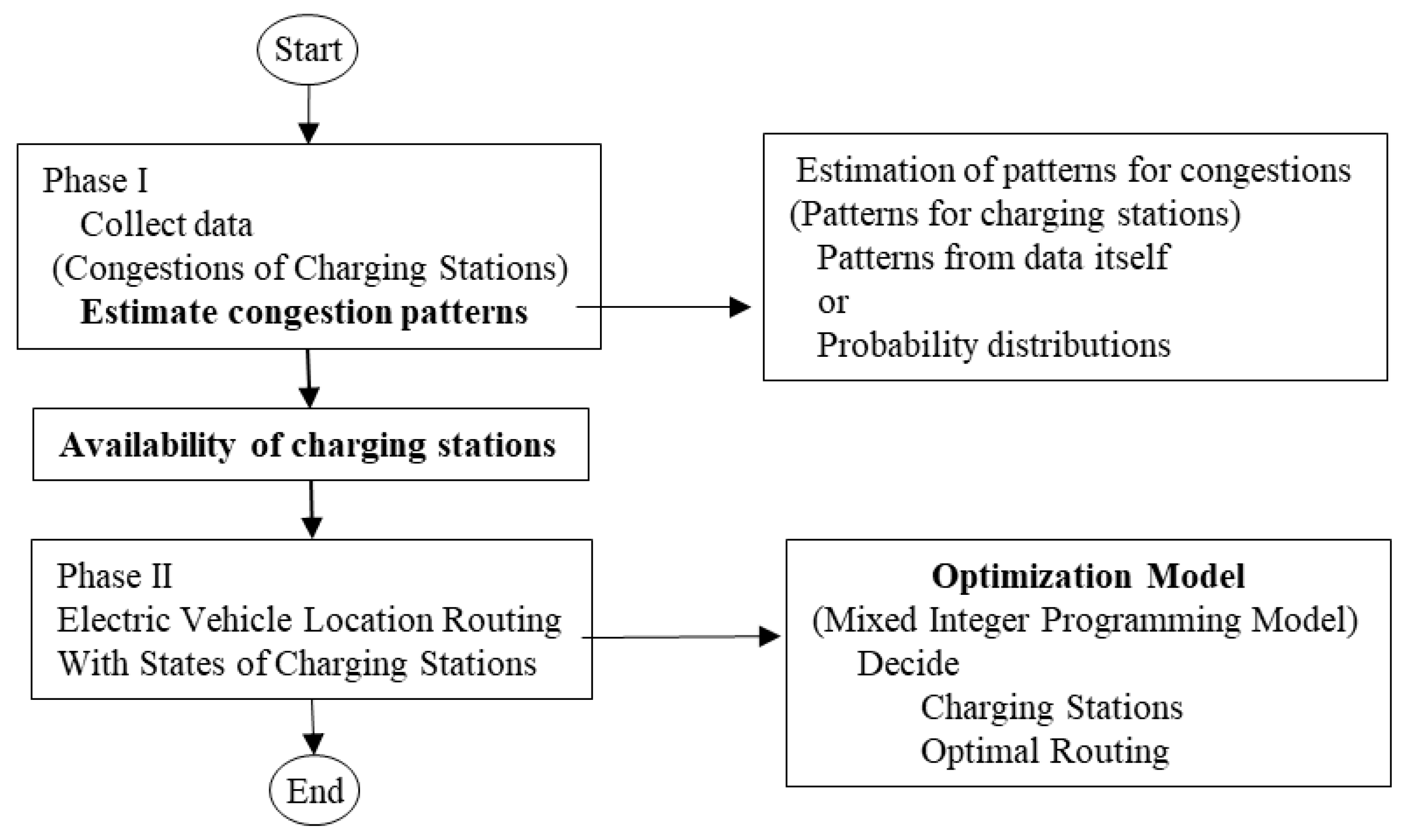
In Figure 3, the problem is solved with two phases. At first, the patterns of states for the charging stations are estimated to present the availability of charging stations. Each charging station has its own pattern for the state of occupation. Upon collecting the data from the charging stations, the patterns are determined by analyzing the data. Once the pattern is found, it can be seen as the availability of the charging station. In the second phase, we solve the electric vehicle routing problem of the model proposed in the previous section. The patterns become the parameters in this routing problem. The solution presents the total travel costs with the states of the charging stations. The solutions for time periods can be used to find the optimal strategy.
The algorithm has been designated to find optimal routing schemes for vehicles. For the problem described in this paper, three algorithms have been adopted to find the solutions of the vehicle routings. The Algorithm 1 randomly chooses the charging time. At the beginning of the day, a random number is generated for each vehicle. If the number is less than 0.5, the vehicle will charge the battery at time period two. Otherwise, the vehicle can charge the battery at time period one.
| Algorithm 1: random solution strategy |
| Initialize: : time horizon for all days : route in period with action where ; where 1 (visit charging station), 0 (no visit charging station) : demand for period in day Repeat: until For day = random(): generate random number [0,1] If If, End |
For the Algorithm 2, total travel distances are considered to make the decisions of charging. Solutions for the vehicle routing problems for period one and two present the total distances of travel for each vehicle. Each vehicle will charge the battery at period one if the total distance of period one is less than the period two.
| Algorithm 2: minimal distance solution strategy |
| Initialize: : time horizon for all days : route in period with action where ; where 1 (visit charging station), 0 (no visit charging station) : demand for period in day Repeat: until For day Solve (EVRP) with : (total distances) Solve (EVRP) with : (total distances) If , If , k→k + 1 End |
The Algorithm 3 considers the states of charging stations in order to find the optimal solution for vehicle routings. In addition to the solutions for vehicle routings for period one and two, the solutions considering the states of the charging stations are also considered to make decisions for the optimal routing strategy.
| Algorithm 3: charging stations solution strategy |
| Initialize: Find states of charging stations : time horizon for all days : route in period with action where ; where 1 (visit charging station), 0 (no visit charging station) : demand for period in day Repeat: until For day Solve (EVRP) with : (objective value) Solve (EVRP) with : (objective value) Solve (EVRP) with and : (objective value) Solve (EVRP) with and : (objective value) If , If , End |
The above algorithms can help vehicles to decide when they should charge. We have compared the results of three algorithms with an example to see their performance.
Table 1 shows the experimental results for the three algorithms with examples which will be shown in Section 5. From the results, the CS algorithm has obtained better solutions than the other algorithms. Each vehicle can visit the charging station only once, minimizing the total travel costs.
For the estimation of the patterns for the states of charging stations, we can derive the probability distribution of the states from the data. The state of a charging station is defined as the time a vehicle must wait when it arrives at the charging station. The data from a charging station may not be the waiting time, so we can derive the waiting time from the dataset. Common data at a station are the number of vehicles that arrive at a certain time. With these data, we can derive the distributions of waiting times at charging stations.
Arrivals to a system are usually assumed as following a Poisson distribution in a queueing system. Let be the parameter of the Poisson distribution and denote the number of events in a given interval. The probability density function is defined as follows.
Function (17) presents the probability that the number of events is in a unit time interval. From the probability distribution of arrivals, we can derive the distribution of the time intervals between arrivals. The probability distribution of the time interval can be defined as an exponential distribution as follows.
Function (18) denotes the probability that the interarrival time between events is . These two probability distributions are used to estimate the states of charging stations. The waiting time of a vehicle is calculated by summing the charging time with the interarrival time. For instance, we assume a simple example for estimating the states from the data.
Table 2 shows the number of vehicles arriving in time intervals. The data can be counted in each charging station. With the data, we can derive the probability distribution of arrivals, which is assumed to follow a Poisson distribution.
Table 3 presents the counts of the arrivals from Table 2. For example, there were zero arrivals five times in Table 1 and two vehicle arrivals occurred three times. The third column is the value of the product of two numbers. With the two sums, we can calculate the of the distribution as follows.
Function (19) presents the calculation of of the distribution of arrivals of vehicles at the charging station. The value of denotes that the average number of vehicles in a unit time period is 1.5. With this , we can derive the interarrival time distribution with the exponential distribution. Thus, the average time of interarrival is calculated as . Adding the charging time from the interarrival can estimate the waiting time of the vehicle.
These estimated waiting times are the parameters for the electric vehicle routing problem as the EVRP model. The routing problem can be solved with the exact algorithm. We show some numerical examples for the routing problem in the next section.
5. Experimental Results
This section presents simple numerical examples for the electric vehicle routing problem. This paper considers an instance modified from a Solomon benchmark problem. The dataset, so-called Solomon benchmark instance, generated by M.M. Solomon (1987, [24]) has been used in many studies into vehicle routing problems; for example, instances.
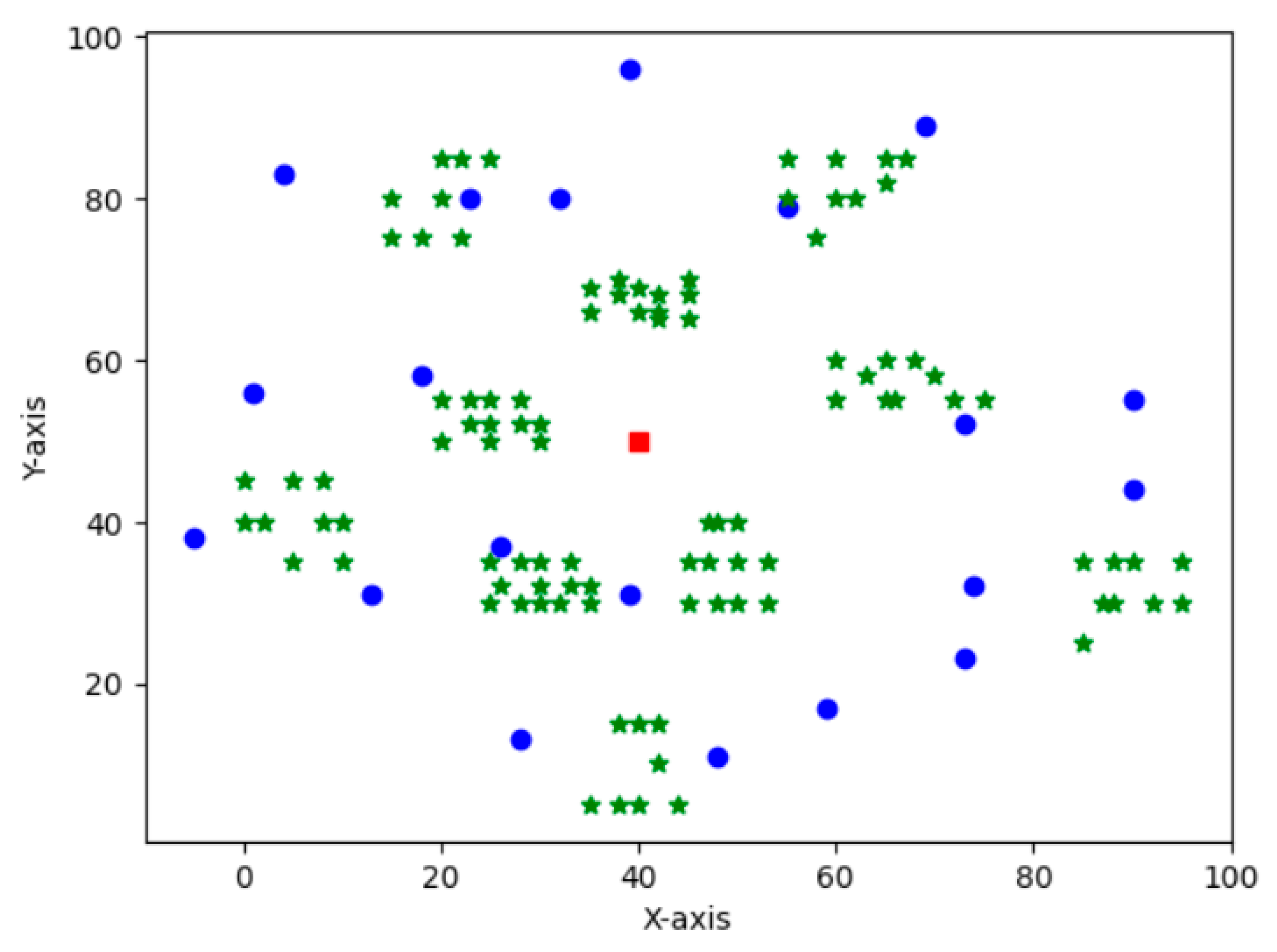
Figure 4 shows an instance for an electric vehicle routing problem. The instance is randomly modified from a Solomon benchmark problem. We have plotted the layout of the instance with the co-ordinates of x and y in the dataset as shown in Figure 4. In the layout, we have not taken into account the route topography since the dataset is generated from the benchmark problem. There is one depot, multiple customer sites, and multiple charging stations. In the figure, the square denotes the depot, circles represent charging stations, and stars represent customer sites. All customer sites have to be visited, but some of the charging stations are selected to visit. A vehicle has to visit a charging station once during the delivery tour.
Solving a mixed integer programming problem with an exact algorithm is a time-consuming task. Thus, we have sampled five small instances from the problem of Figure 4, reducing the size to 15 customer sites. Figure 5 shows the sample example one from the instance in Figure 4, so the instance has one depot, 21 potential charging stations, and 15 customer sites for each time period. Vehicles have to service all customer sites for two time periods and charge either in period one or period two. Potential charging stations are selected to minimize the total travel costs.
In this paper, we have implemented the EVRP model with C# with the concert technology of the CPLEX 12.6.1 software. Solving the instance in Figure 5 for period one and period two, we have the following results.
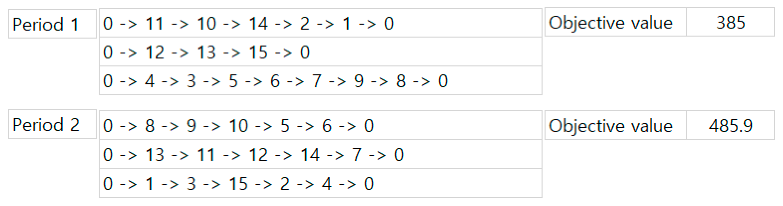
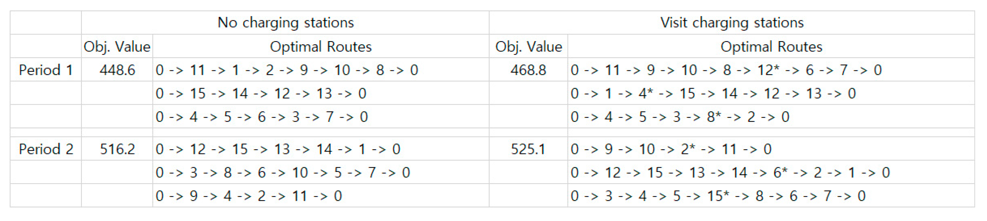
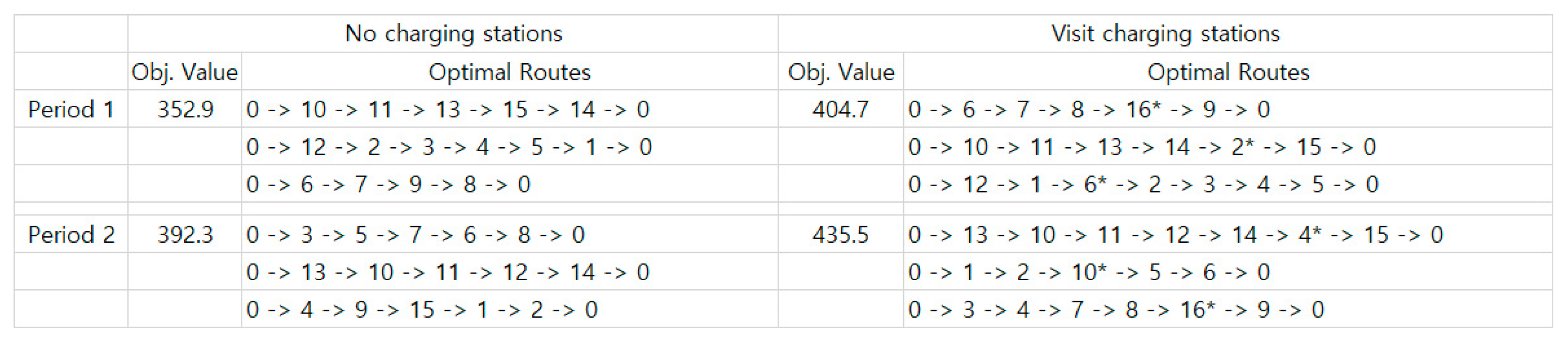
Figure 6 and Figure 7 show the solution of example one. The numbers in each row denote the nodes of the depot (0), charging stations, and customer sites. The order of the node numbers in a row presents the sequence of the optimal route. The sequence of nodes in a row is for the route of each vehicle. The vehicle starts from depot node 0 and returns to the depot. The objective value is the total cost of each route. The total cost is calculated with the sum of the total distances of the routes and costs of reaching the charging stations. Three vehicles are used to service the customer sites. In Figure 6, vehicles travel without visiting charging stations. On the other hand, vehicles are visiting charging stations once in Figure 7 and the number with an asterisk presents the charging station the vehicle visits. From the results, it can be seen that the optimal routes are changed when the vehicles visit the charging stations. The objective values as total travel costs are also changed. For the optimal strategy, we can calculate and and compare them.
From comparison (20), is less than . Accordingly, vehicles are recommended to visit charging stations in period two rather than period one.
The results of Figure 6 without visiting charging stations can be seen as the routing from fossil-fueled vehicles. The results of Figure 7 from electric vehicles have 6% more total distances than the results of Figure 6. However, for the emission of CO2, the results of traditional routing solutions are much larger than the results of the optimal routings from Figure 7.
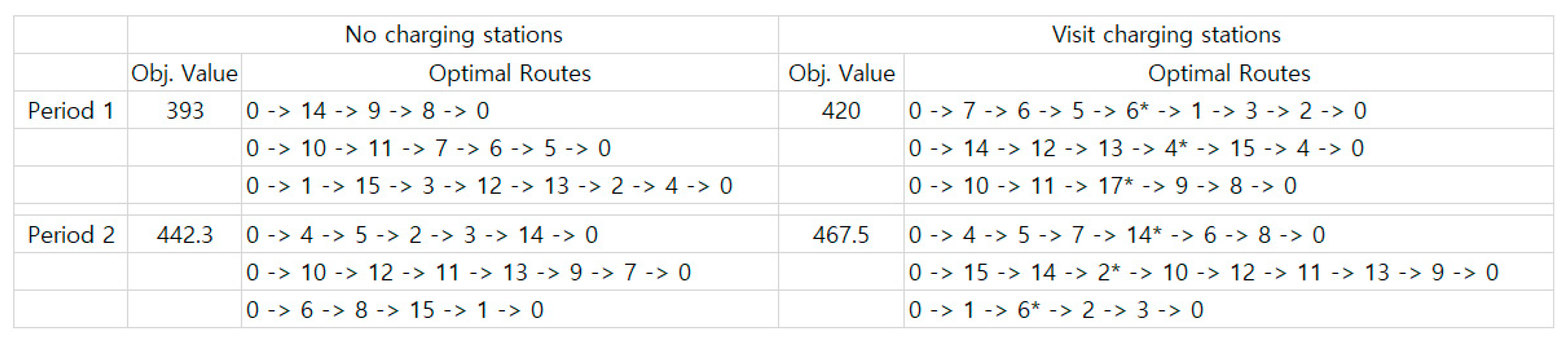
Figure 8, Figure 9, Figure 10 and Figure 11 show the experimental results of examples 2~5. The examples are generated by randomly sampling 15 customer sites from the instance in Figure 4. Optimal routes are determined by solving the EVRP model with the exact method. For the strategy for a day, we calculate and for each example.
Equations (21)–(24) present the comparisons of total travel costs for the days. In examples two, three, and four, the total travel costs of are smaller than . Thus, in case of examples two, three, and four, visiting the charging stations in period two is better than the other way. On the other hand, for example five, it is better for vehicles to visit the charging stations in period one. In this way, we can make decisions how and when the vehicles take charging during the delivery tours.
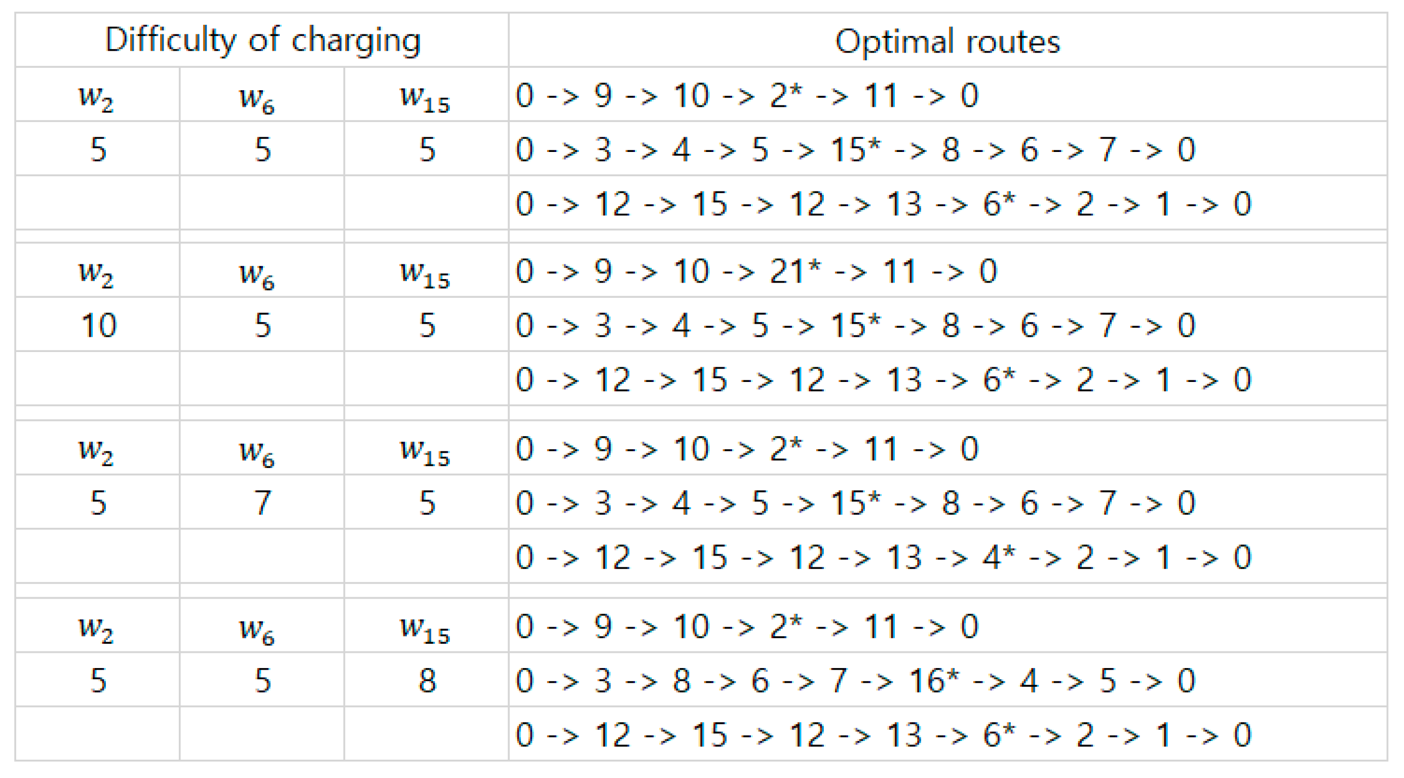
Figure 12 presents the solutions as the difficulties of charging at the stations change. The difficulty of charging is the weight in the objective function of the EVRP model. As the difficulty changes, the optimal route changes. If the change is small, the optimal solution does not change. However, if the change is big enough, the optimal route will be different. The model can find the threshold of the difficulty to change the optimal routes. Thus, with the values, we can control the routing strategy for vehicles.
Depending on the battery state or charger’s power output or other factors, the charging times vary in some charging stations. The variability of the charging times may affect the routing solutions. We have conducted the sensitivity analysis to show how the changes in the charging times affect the routing solutions.
Table 4 shows the sensitivity analysis of charging times and routing solutions. In total, 21 potential charging stations are divided into three groups: 1~7, 8~14, and 15~21. We have assigned the charging times differently to those three groups to see the changes to the routing solutions. As the charging times in only a certain group increase, the charging stations in that group have not been used in the optimal routes.
6. Conclusions
This paper suggests the electric vehicle routing problem by considering the states of charging stations. The issue of charging is important for the electric vehicle routing problem. Charging functions, energy consumption, and the location of charging stations have been explored in many studies. However, the state of a charging station is also important to find the optimal route in the electric vehicle routing problem. The state of a charging station can be seen as the availability of the charging station. If charging is not available when a vehicle arrives, the travel costs will significantly increase. In this paper, we consider the states of charging stations, formulate the model, and suggest the solution approach.
The first step of the solution approach is to collect the data from all charging stations. The arrivals of vehicles to the station are collected as raw data. The data has been analyzed to find the patterns of states of the charging stations. Estimating the probability distribution of arrivals and interarrival times can be used to find the pattern of waiting times when a vehicle arrives at the charging station. Once the patterns of the states of charging stations are determined, the values are used as input parameters for the model of the electric vehicle routing problem. With the solutions, we can find the optimal routing strategy for the two-time-period problem.
Experimental results provide how to find the optimal strategy for the electric vehicle routing problem with the states of charging stations. In the two-time-period problem, we are able to determine in which time period the vehicles visit the charging stations. The difficulty of charging can be used to find the threshold where the optimal routes change. Thus, we can control the electric vehicle routing by considering the availability of the charging stations.
The nonstationary distributions for the states of charging stations should be explored in future work. Investigating the uncertainty of charging durations for vehicles is also a challenging issue. Obtaining real-world scenarios for the states of charging stations and investigating the charging behaviors of vehicles are the future works of our study. In addition, the change in atmospheric conditions, especially temperature, change of topography (driving uphill or downhill), or carried weight have a significant impact on the operation of batteries and thus the range of electric vehicles. Taking into account these parameters is also future work.
Funding
This work was supported by the National Research Foundation of Korea (NRF) grant funded by the Korea government (MSIT) (No. 2021R1A2C1014180).
Institutional Review Board Statement
Not applicable.
Informed Consent Statement
Not applicable.
Data Availability Statement
No new data were created or analyzed in this study. Data sharing is not applicable to this article.
Conflicts of Interest
The authors declare no conflict of interest.
References
- Xiao, Y.; Zhang, Y.; Kaku, I.; Kang, R.; Pan, X. Electric vehicle routing problem: A systematic review and a new comprehensive model with nonlinear energy recharging and consumption. Renew. Sustain. Energy Rev. 2021, 151, 111567. [Google Scholar] [CrossRef]
- Chakraborty, N.; Mondal, A.; Mondal, S. Intelligent charge scheduling and eco-routing mechanism for electric vehicles: A multi-objective heuristic approach. Sustain. Cities Soc. 2021, 69, 102820. [Google Scholar] [CrossRef]
- Schneider, M.; Stenger, A.; Hof, J. An adaptive VNS algorithm for vehicle routing problems with intermediate stops. OR Spectr. 2015, 37, 353–387. [Google Scholar] [CrossRef]
- Keskin, M.; Laporte, G.; Çatay, B. Electric Vehicle Routing Problem with Time-Dependent Waiting Times at Recharging Stations. Comput. Oper. Res. 2019, 107, 77–94. [Google Scholar] [CrossRef]
- Hiermann, G.; Puchinger, J.; Ropke, S.; Hartl, R.F. The Electric Fleet Size and Mix Vehicle Routing Problem with Time Windows and Recharging Stations. Eur. J. Oper. Res. 2016, 252, 995–1018. [Google Scholar] [CrossRef]
- Montoya, A.; Guéret, C.; Mendoza, J.E.; Villegas, J.G. The electric vehicle routing problem with nonlinear charging function. Transp. Res. Part B Methodol. 2017, 103, 87–110. [Google Scholar] [CrossRef]
- Froger, A.; Mendoza, J.E.; Jabali, O.; Laporte, G. Improved formulations and algorithmic components for the electric vehicle routing problem with nonlinear charging functions. Comput. Oper. Res. 2019, 104, 256–294. [Google Scholar] [CrossRef]
- Bac, U.; Erdem, M. Optimization of electric vehicle recharge schedule and routing problem with time windows and partial recharge: A comparative study for an urban logistics fleet. Sustain. Cities Soc. 2021, 70, 102883. [Google Scholar] [CrossRef]
- Basso, R.; Kulcsár, B.; Sanchez-Diaz, I. Electric vehicle routing problem with machine learning for energy prediction. Transp. Res. Part B Methodol. 2021, 145, 24–55. [Google Scholar] [CrossRef]
- Kasani, V.S.; Tiwari, D.; Khalghani, M.R.; Solanki, S.K.; Solanki, J. Optimal Coordinated Charging and Routing Scheme of Electric Vehicles in Distribution Grids: Real Grid Cases. Sustain. Cities Soc. 2021, 73, 103081. [Google Scholar] [CrossRef]
- Ma, B.; Hu, D.; Chen, X.; Wang, Y.; Wu, X. The vehicle routing problem with speed optimization for shared autonomous electric vehicles service. Comput. Ind. Eng. 2021, 161, 107614. [Google Scholar] [CrossRef]
- Pelletier, S.; Jabali, O.; Laporte, G. The electric vehicle routing problem with energy consumption uncertainty. Transp. Res. Part B: Methodol. 2019, 126, 225–255. [Google Scholar] [CrossRef]
- Al-dal’ain, R.; Celebi, D. Planning a mixed fleet of electric and conventional vehicles for urban freight with routing and replacement considerations. Sustain. Cities Soc. 2021, 73, 103105. [Google Scholar] [CrossRef]
- Brady, J.; O’Mahony, M. Modelling charging profiles of electric vehicles based on real-world electric vehicle charging data. Sustain. Cities Soc. 2016, 26, 203–216. [Google Scholar] [CrossRef]
- Schneider, M.; Stenger, A.; Goeke, D. The Electric Vehicle-Routing Problem with Time Windows and Recharging Stations. Transp. Sci. 2014, 48, 500–520. [Google Scholar] [CrossRef]
- Nolz, P.C.; Absi, N.; Feillet, D.; Seragiotto, C. The consistent electric-Vehicle routing problem with backhauls and charging management. Eur. J. Oper. Res. 2022, 302, 700–716. [Google Scholar] [CrossRef]
- Alizadeh, M.; Wai, H.T.; Scaglione, A.; Goldsmith, A.; Fan, Y.Y.; Javidi, T. Optimized path planning for electric vehicle routing and charging. In Proceedings of the 2014 52nd Annual Allerton Conference on Communication, Control, and Computing (Allerton), Monticello, IL, USA, 30 September–3 October 2014; pp. 25–32. [Google Scholar]
- Lu, J.; Wang, L. A Bi-Strategy Based Optimization Algorithm for the Dynamic Capacitated Electric Vehicle Routing Problem. In Proceedings of the 2019 IEEE Congress on Evolutionary Computation (CEC), Wellington, New Zealand, 10–13 June 2019; pp. 646–653. [Google Scholar]
- Gan, L.; Topcu, U.; Low, S.H. Optimal decentralized protocol for electric vehicle charging. IEEE Trans. Power Syst. 2013, 28, 940–951. [Google Scholar] [CrossRef]
- Kessler, L.; Bogenberger, K. Dynamic Traffic Information for Electric Vehicles as a Basis for Energy-Efficient Routing. Ransportation Res. Procedia 2015, 37, 457–464. [Google Scholar] [CrossRef]
- Luo, Q.; Ye, Z.; Jia, H. A Charging Planning Method for Shared Electric Vehicles with the Collaboration of Mobile and Fixed Facilities. Sustainability 2023, 15, 16107. [Google Scholar] [CrossRef]
- Wang, Y.; Zhou, J.; Sun, Y.; Wang, X.; Zhe, J.; Wang, H. Electric Vehicle Charging Station Location-Routing Problem with Time Windows and Resource Sharing. Sustainability 2022, 14, 11681. [Google Scholar] [CrossRef]
- Jeong, J.; Ghaddar, B.; Zufferey, N.; Nathwani, J. Adaptive robust electric vehicle routing under energy consumption uncertainty. Transp. Res. Part C Emerg. Technol. 2024, 160, 104529. [Google Scholar] [CrossRef]
- Solomon, M.M. Algorithms for the Vehicle Routing and Scheduling Problems with Time Window Constraints. Oper. Res. 1987, 35, 254–265. [Google Scholar] [CrossRef]
Figure 1.
Electric vehicle routing problem.

Figure 2.
Two delivery tours in a day.

Figure 3.
Solution procedure.

Figure 4.
Instance of an electric vehicle routing problem.

Figure 5.
Instance example one for Periods One and Two in a day.

Figure 6.
Solution of example one not visiting charging stations.

Figure 7.
Solution of example one visiting charging stations.

Figure 8.
Solution of example two.

Figure 9.
Solution of example three.

Figure 10.
Solution of example four.

Figure 11.
Solution of example five.

Figure 12.
Solutions depending on the states of charging stations.


Table 1.
Total costs for three algorithms.
| Days | Algorithm 1 | Algorithm 2 | Algorithm 3 |
|---|---|---|---|
| 1 | 922.3 | 922.3 | 874.0 |
| 2 | 943.7 | 963.9 | 943.7 |
| 3 | 788.4 | 840.2 | 788.4 |
| 4 | 862.3 | 862.3 | 860.5 |
| 5 | 746.3 | 825.0 | 742.5 |
| Sum | 4263.0 | 4413.7 | 4209.1 |
Table 2.
Arrival of vehicles in time intervals.
| Time Interval | Arrivals of Vehicles | Time Interval | Arrivals of Vehicles |
|---|---|---|---|
| 11:00–11:10 | 1 | 12:20–12:30 | 1 |
| 11:10–11:20 | 0 | 12:30–12:40 | 2 |
| 11:20–11:30 | 0 | 12:40–12:50 | 1 |
| 11:30–11:40 | 0 | 12:50–13:00 | 0 |
| 11:40–11:50 | 1 | 13:00–13:10 | 4 |
| 11:50–12:00 | 2 | 13:10–13:20 | 0 |
| 12:00–12:10 | 3 | 13:20–13:30 | 2 |
| 12:10–12:20 | 4 |
Table 3.
Count of arrivals.
| Number of Arrivals (A) | Observed Counts (B) | A × B |
|---|---|---|
| 0 | 5 | 0 |
| 1 | 4 | 4 |
| 2 | 3 | 6 |
| 3 | 1 | 3 |
| 4 | 2 | 8 |
| Sum | 14 | 21 |
Table 4.
Sensitivity analysis: charging times affect the routing solutions.
| Charging Stations | 1~7 | 8~14 | 15~21 | Charging Stations Used in the Optimal Routes for Three Vehicles |
|---|---|---|---|---|
| Charging times | 5 | 5 | 5 | 4, 8, 17 |
| 10 | 5 | 5 | 4, 8, 17 | |
| … | 5 | 5 | 4, 8, 17 | |
| 35 | 5 | 5 | 4, 8, 17 | |
| 40 | 5 | 5 | 8, 14, 21 | |
| 45 | 5 | 5 | 8, 14, 21 | |
| 5 | 5 | 5 | 4, 8, 17 | |
| 5 | 10 | 5 | 4, 6, 17 | |
| 5 | 15 | 5 | 4, 6, 17 | |
| 5 | 5 | 5 | 4, 8, 17 | |
| 5 | 5 | 10 | 4, 8, 17 | |
| 5 | 5 | 15 | 4, 8, 14 | |
| 5 | 5 | 20 | 4, 8, 14 |
Disclaimer/Publisher’s Note: The statements, opinions and data contained in all publications are solely those of the individual author(s) and contributor(s) and not of MDPI and/or the editor(s). MDPI and/or the editor(s) disclaim responsibility for any injury to people or property resulting from any ideas, methods, instructions or products referred to in the content. |
© 2024 by the author. Licensee MDPI, Basel, Switzerland. This article is an open access article distributed under the terms and conditions of the Creative Commons Attribution (CC BY) license (https://creativecommons.org/licenses/by/4.0/).
Share and Cite
MDPI and ACS Style
Kim, G. Electric Vehicle Routing Problem with States of Charging Stations. Sustainability 2024, 16, 3439. https://doi.org/10.3390/su16083439
AMA Style
Kim G. Electric Vehicle Routing Problem with States of Charging Stations. Sustainability. 2024; 16(8):3439. https://doi.org/10.3390/su16083439
Chicago/Turabian StyleKim, Gitae. 2024. "Electric Vehicle Routing Problem with States of Charging Stations" Sustainability 16, no. 8: 3439. https://doi.org/10.3390/su16083439
Note that from the first issue of 2016, this journal uses article numbers instead of page numbers. See further details here.