
Influence of Urban Railway Network Centrality on Residential Property Values in Bangkok
by
 , , and
Varameth Vichiensan
1,2,*,
Vasinee Wasuntarasook
3,
Titipakorn Prakayaphun
4,
Masanobu Kii
5 and
Yoshitsugu Hayashi
6 1
Department of Civil Engineering, Faculty of Engineering, Kasetsart University, Bangkok 10900, Thailand
2
Center for Logistics Engineering Technology and Management, Faculty of Engineering, Kasetsart University, Bangkok 10900, Thailand
3
Graduate School, Kasetsart University, Bangkok 10900, Thailand
4
Department of Constructional Engineering, Graduate School of Engineering, Chubu University, Kasugai 487-8501, Japan
5
Graduate School of Engineering, Osaka University, Osaka 565-0871, Japan
6
Center for Sustainable Development and Global Smart City, Chubu University, Kasugai 487-8501, Japan
*
Author to whom correspondence should be addressed.
Sustainability 2023, 15(22), 16013; https://doi.org/10.3390/su152216013
Submission received: 28 September 2023
/
Revised: 6 November 2023
/
Accepted: 14 November 2023
/
Published: 16 November 2023
(This article belongs to the Special Issue Integrating Sustainable Transport and Urban Design for Smart Cities)
Abstract
:In recent decades, Bangkok has experienced substantial investments in its urban railway network, resulting in a profound transformation of the city’s landscape. This study examines the relationship between railway development and property value uplift, particularly focusing on network centrality, which is closely linked to urban structure. Our findings are based on two primary analyses: network centrality and spatial hedonic models. The network centrality analysis reveals that closeness centrality underscores the city’s prevailing monocentric structure, while the betweenness centrality measure envisions the potential emergence of urban subcenters. In our hedonic analysis of condominiums near railway stations, we formulated various regression models with different specifications, incorporating spatial effects and network centrality. With Bangkok’s predominant monocentric structure in mind, we found that the spatial regression model, including a spatial error specification and closeness centrality, outperforms the others. This suggests that the impact of railways on property values extends beyond station proximity and encompasses network centrality, intricately linked with the city’s urban structure. We applied our developed model to estimate the expected increase in property values at major interchange stations with high network centralities. These numerical values indicate a considerable potential for their evolution into urban subcenters. These insights offer valuable policy recommendations for effectively harnessing transit-related premiums and shaping the future development of both the railway system and the city.
1. Introduction
Historically, Bangkok has been characterized as a monocentric city [1], featuring a sprawling central business district (CBD) that houses diverse urban activities, primarily within the bounds of the circumferential subway’s blue line. However, inefficiencies in land use planning and control have resulted in the city’s expansion alongside highways to its outskirts, where opportunities for employment, education, and healthcare are often limited. Adding to the rapid suburbanization are public transport deficiencies, particularly concerning first- and last-mile connectivity, which affect the convenience of using public transportation. This has led to a heavy reliance on private automobiles, causing severe traffic congestion during peak hours, both entering and leaving the city center. Consequently, issues such as increased fuel consumption and air pollution, including the presence of PM2.5 particles, have arisen.
To address these challenges, Bangkok has made significant investments in developing railways over the past three decades, with the first railway line opened in 1999. The current rail transit master plan (M-Map) aims to complete 12 lines, covering a total distance of 509 km by 2029 [2]. Furthermore, preparations are underway for the second mass rapid transit master plan (M-Map2), which will include additional railway lines traversing the metropolitan area. The overarching vision is for Bangkok to evolve into a polycentric city with subcenters at major hubs interconnected by railways [3].
The railway developments have stimulated real estate development along the railway lines, substantially reshaping the urban landscape. While many properties near railway stations along the railway lines in the central area often appreciate, those located along certain sections, such as the purple line or those at a greater distance from the city center, may not experience the same level of value increase [4]. Therefore, the impact of railway network development on property value across the entire metropolitan area remains a subject of ongoing investigation.
We hypothesize that the influence of railways on property value is not solely due to station proximity; the railway network structure also plays a substantial role. While the influence of station proximity has been extensively examined, the specific impact of railway network structure in this context remains underexplored. Our aim is to investigate the intricate relationship between railway development and property value uplift through railway network centrality, which is closely associated with urban structure.
This study has two primary objectives. Firstly, it aims to assess the centrality of Bangkok’s railway network and trace its evolution over the past decade, applying various centrality measures. Secondly, it aims to analyze how the railway network influences real estate values through spatial econometric models. These models incorporate spatial effects and take into account not only station proximity but also network centrality, which is intricately associated with urban structure, in addition to the conventional explanatory attributes.
Ultimately, our goal is to determine the intrinsic value of the railway network that underlines property values and provide policy recommendations for capturing transit premiums and guiding future railway and urban development to achieve sustainable development goals.
The organization of this study is illustrated in Figure 1, and the sequence of topics presented in this paper is as follows. The subsequent section presents literature reviews. Section 3 describes the method used to determine network centrality, employing four centrality measures, and introduces the hedonic regression models, which involve enhancing an ordinary least square regression model through the incorporation of spatial effects. Section 4 provides an overview of the urban railway network in Bangkok and presents the results of the centrality analysis, showcasing the evolution of network centralities within the Bangkok railway network over the past decade. Section 5 details the hedonic analysis, including data, variables, estimation results, and model applications to forecast an increase in property value along upcoming railway lines. Section 6 offers discussions. Section 7 offers valuable insights into policy implications. Finally, in Section 8, the paper concludes by summarizing the findings and contributions of the study.
2. Literature Reviews
2.1. Influences of Urban Railways on Property Value
Urban railways have a profound influence on urban development, affecting various aspects of a city’s growth, infrastructure, economy, and overall quality of life. They promote multi-centered or polycentric development by enhancing land use and population density as well as accessibility to different parts of the city [5,6,7]. Urban railways also play a crucial role in alleviating traffic congestion [8] and curbing urban sprawl [9]. By providing an attractive alternative to car-based commuting, they reduce vehicle kilometers traveled and contribute to improved traffic flow, shorter commute times, and reduced pollution. However, some studies found railways having varying effects at some locations within station buffer areas [10].
One of the significant impacts of urban railways is the uplift in land value and/or property value [4,11,12,13]. Proximity to railway stations typically leads to increased property values [14,15]. This effect can significantly influence property values, rendering areas served by rail transit systems more attractive to both residents and investors [16]. The influence of rail transit on property value may vary at different stages of the project. In Hong Kong, a study reported a continuous increase in property values since the construction was announced, with values even rising further after the project began [17]. In contrast, a study in Sydney found a negative impact during the project announcement phase but observed a positive trend after construction commenced [18].
However, it is worth noting that during the COVID-19 pandemic, the advantage of living near a railway station in Chengdu’s metro system was observed to decline due to the declining role of the metro [19]. To quantify the benefit of rail transit on land or property values, the hedonic approach has been widely employed [10,14,20].
2.2. Influence of Network Centrality on Property Value
Network centrality, a concept in network theory, evaluates the importance of nodes within a network. It encompasses various measures, including degree centrality, betweenness centrality, closeness centrality, eigenvector centrality, and PageRank. Network centrality analysis finds applications in diverse fields, such as social network analysis, information science, and transportation analysis. Highly central transportation nodes, including roads, railways, or waterways, often serve as pivotal hubs, enhancing the efficient movement of passengers and goods.
In the context of railway network centrality analysis, previous studies have employed various centrality measures, yielding implications for railway network development, operation, and management. For instance, one study assessed 28 metro systems worldwide using betweenness centrality, leading to recommendations for mitigating overcrowding [21]. Another study in Shanghai compared urban railway stations using degree, closeness, and betweenness centralities, offering operational insights [22]. In Hong Kong, the rapid transit network’s evolution was ranked based on centrality measures, guiding station management and maintenance [23]. Stockholm’s urban railway network was evaluated using degree, closeness, and betweenness centralities [24], while regional and intercity railways, including China’s high-speed rail network, were assessed and grouped by centrality measures [25].
Furthermore, certain studies have explored the association between transport network centrality and other factors. Tokyo discovered a strong relationship between railway network centrality and ridership [26]. In Beijing, bus networks exhibited a high correlation with passenger flow based on centrality measures [27]. Moreover, railway network centrality has been associated with subcenter formation in polycentric cities [28].
While there are numerous studies on the impact of road network centrality, such as [29,30,31], there are relatively few studies examining the influence of railway network centrality on property values in certain cities. For instance, in Hong Kong, the influence of closeness centrality was explored [32], and in Shanghai, the focus was on degree centrality [33]. In the Scania region, the most southern region of Sweden, a study found that the centrality of the regional train network, specifically degree and closeness centralities, influenced single-family house prices, though betweenness centrality did not show a statistically significant influence [34]. On a larger scale, the centrality of China’s high-speed rail network was also found to affect land values and housing prices [35,36].
2.3. Hedonic Price Model
A hedonic price model refers to an econometric model used to estimate the relationship between the price of a product or service and the various attributes or characteristics that influence that price. Hedonic price models are widely used in economics and marketing to understand how consumers make choices and how prices are determined in markets with differentiated products. They are also used for various purposes, including assessing the impact of environmental attributes on property values, predicting the price of new products, and conducting cost–benefit analyses for public policy decisions.
In the context of real estate, a hedonic price model serves as a valuable tool to assess how various factors, such as location, size, the number of bedrooms, and other features, impact the price of a house or condominium unit. By analyzing a dataset of property values along with their attributes, the model provides insights into the value that buyers place on each of these characteristics.
The hedonic price model typically treats the value of real estate property as a dependent variable, influenced by its constituent attributes or characteristics, which serve as explanatory variables. Dependent variables can take various forms, including the advertised or listed price [37,38], assessed value [39], or the actual sale transaction price [11,40,41,42,43,44]. Explanatory variables are often categorized into four main groups: structural characteristics, locational characteristics, neighborhood characteristics, and transport accessibility [45].
Structural characteristics encompass various aspects of the property, including its size, age, room types, number of bedrooms, and building-related features such as the building’s height, car parking availability, shared facilities, and more.
Locational characteristics involve factors related to the property’s proximity to urban or town centers, which may include the central business district (CBD) [14,15,46,47,48] or subcenters [43,45,49,50,51], as well as proximity or accessibility to essential services like education, healthcare, public parks, retail options, and more.
Neighborhood characteristics pertain to the area’s features in the vicinity, often including activities such as employment or retail shops, along with attributes associated with transit-oriented development (TOD) environments. These attributes may include mixed land use or mixed activities [49,52,53], land use intensity [45], job–housing balance, or the density of certain population groups [12,54].
Transport accessibility factors encompass the proximity to various transportation facilities, including rail transit stations [11,37,55,56], rail services [48], bus stops [57,58], bike-sharing stations [58], bus frequency [59], major highways, and more. The proximity of a rail transit station could be measured in various ways, such as Euclidean or straight-line distance [47,48,54,60,61], distance along transportation networks [41,49,62], or other impedance measures, like travel time [40]. Furthermore, the quality of railway services, which includes factors like train frequency, travel time between stations, and overall travel convenience, has been shown to have a substantial impact on property value [48,59,63].
2.4. Regression Model with Spatial Effects
Spatial effects refer to the influence of the spatial arrangement or location of data points on the dependent variable. These effects can manifest in two primary forms: spatial dependence and spatial heterogeneity [64,65]. Spatial dependence pertains to the spatial relationship between values of a variable for two locations that are some distance apart. Spatial heterogeneity, on the other hand, relates to the uneven distribution of a variable’s values across space. These spatial effects can be incorporated into the hedonic price model through various techniques, including spatial lag models, spatial error models, combined spatial lag and error models, and geographically weighted regression models.
The spatial lag model takes into consideration the spatial dependencies among observations by introducing a lagged dependent variable as an additional explanatory variable in the regression model [10,11,29,49,58,66]. This lagged variable represents the average value of the dependent variable in neighboring locations, effectively acknowledging that the value of the dependent variable in one location may be influenced by the values in nearby locations. Conversely, the spatial error model considers that there is spatial autocorrelation in the error terms of the regression model, so the spatial autocorrelation is explicitly incorporated into the error term through spatially weighted values derived from nearby observations [20,34,67]. This model acknowledges that observations in close proximity may share unobserved characteristics that impact the dependent variable. Moreover, centrality was found to be incorporated in regression in both ways: spatial lag and spatial error models, for example [31,34]. Both the spatial lag model and spatial error model yield a unified set of variable coefficients and spatial parameters across the entire study area, categorizing them as global models.
In contrast to these global models, geographically weighted regression (GWR) represents a spatial regression technique that accommodates variations in the relationship between the dependent variable and explanatory variables across different spatial locations [4,43,48,61,62,68,69]. This phenomenon, known as nonstationarity, implies that parameter estimates vary across the study area [70]. Instead of estimating a single set of coefficients for the entire dataset, GWR computes a distinct set of coefficients for each location. This approach allows for the capture of spatial heterogeneity in the relationships between variables, making GWR a family of local models. GWR has been employed as a hedonic price model to examine the influence of rail transit on property value [4,42,48,71,72].
3. Methods
3.1. Network Centrality Measures
Network centrality measures indicate the importance of a node within the total network. Among various forms, this study considered railway network centrality based on four centrality measures: degree, closeness, betweenness, and eigenvector centralities. Firstly, degree centrality is the simplest measure of centrality, which counts the number of links connected to each node .
where if and are connected by a link; 0 otherwise. Secondly, closeness centrality is the average length of the shortest path between the node and the other nodes in the network.
where is the number of nodes in the network. Thirdly, betweenness centrality for each node is the number of the shortest paths that pass through the node, i.e., it captures which nodes are important in the flow of the network.
where is the total number of shortest paths from node to node and is the number of those paths that pass through node . Fourthly, eigenvector centrality is determined from the principal eigenvector of the adjacency matrix , where if node is linked to node .
where is the set of neighbors of node and is an eigenvalue, obtained from the eigenvector equation . If a node is pointed to by many nodes, which also have high eigenvector centrality, that node will have high eigenvector centrality.
As the urban railway network in Bangkok has developed over the past years, we assessed railway network centrality at three different time points: 2016, 2021, and 2026, respectively. To perform these calculations and visualize the results, we employed, Gephi, an open-source software for network analysis [73].
3.2. Hedonic Regression Models
This study employs a hedonic pricing model to analyze the influence of individual factors on property values. The concept of hedonic value, commonly used in economics and real estate, explains how a property’s price is influenced by various attributes or characteristics. In real estate, these attributes encompass factors such as location, size, amenities, access to transportation, proximity to services, etc.
Hedonic models provide clear and interpretable coefficients for each variable, enabling a straightforward understanding of how factors influence property values [74]. We aim to maintain simplicity and ensure that our analysis remains robust and comprehensible. Emphasizing simplicity is crucial to keep the analysis accessible and actionable for stakeholders. Additionally, hedonic models enable the integration of domain knowledge and expert insights, ensuring that factors known to impact property values are appropriately considered. They tend to be more stable and less susceptible to overfitting compared to complex AI-based methods, which may excel in training data but perform poorly on new data. Moreover, hedonic models facilitate statistical inference, allowing for the assessment of the statistical significance of coefficients and hypothesis testing regarding variable relationships.
In this paper, we introduce hedonic regression models that extend ordinary least squares regression (OLS) by incorporating spatial dependence through the inclusion of spatial-lagged and spatial error terms. Each of these models is described below.
- OLS model
The hedonic regression model is specified as follows.
where is a vector () of observations corresponding to a dependent variable, is a matrix () of observations of k independent variables, is a vector () of regression parameters, and is a vector () of errors that are assumed to be normally distributed.
The ordinary least square (OLS) estimation is referred to as a Best Linear Unbiased Estimator (BLUE). The OLS estimate is obtained by minimizing the sum of squared prediction errors. Assumptions regarding the random error include its normal distribution with a mean of zero or and a constant, uncorrelated variance (homoscedasticity) or . The OLS estimates for the coefficients are obtained as .
However, the above assumptions may not always hold true in situations in which properties that are geographically close to each other might have similar prices due to shared neighborhood characteristics, transportation accessibility, and other local factors. Spatial dependence emerges when the observed value at a particular location is influenced by the values observed in nearby locations. Spatial data commonly exhibit spatial dependence in both its variables and error terms. When this is the case, the independence assumption of OLS is violated, and the errors in the model are likely correlated, leading to inefficient OLS estimates.
- 2.
- Spatial lag model
A spatial autoregressive model, often referred to as a spatial lag model, is obtained by including a function of the dependent variable observed at other locations as follows.
where is the autoregressive parameter of the lag variable, is the spatial weight for i and j, and the error term is i.i.d. The weighting function can be in different forms, such as the inverse function () and the negative exponential function (), where α and β are parameters [41]. The Equation (7) could be written in matrix form as:
where W is the () spatial weight matrix.
- 3.
- Spatial error model
A spatial error model is obtained by specifying the covariance structure of the random disturbance terms, i.e., . In the context of the hedonic price model, neighborhood effects that are difficult to quantify are shared by nearby properties and appear as spatially correlated errors. A spatial autoregressive error model, shortly referred to as a spatial error model, specifies the error structure as:
where is the autoregressive parameter of the error and as a random error term, which is typically assumed to be independently and identically distributed. The Equation (9) could be written in matrix form as:
4. Network Centrality Analysis
4.1. Urban Railway Network in Bangkok
The study area covers the Bangkok metropolitan region (BMR), including Bangkok, the capital city under the Bangkok Metropolitan Administration (BMA), and five surrounding provinces: Nonthaburi, Nakhon Pathom, Pathum Thani, Samut Prakan, and Samut Sakhon. The development of urban railways in this region aligns with the mass transit development master plan, known as the M-Map. In 2021, when we collected residential property data, eight urban railway lines were operational: light green, dark green, blue, purple, airport rail link, light red, dark red, and gold lines. There were 203 stations: 112 were already operational and 91 were under construction. Figure 2 provides an illustration of the railway network and station status as of 2021.
The yellow and pink lines faced COVID-19-related delays and were rescheduled to begin service in 2023, while the orange line, delayed due to contract issues, is not expected to start operations before 2025. Several extensions are in the planning or tendering stages but have not yet started construction. These extensions include the south section of the purple line, the west section of the orange line, the inner segments of the light red line, and the east section of the dark red lines. These extensions were not considered in this study because their station locations were not finalized, and their impact on property values was deemed insignificant. The entire system is projected to be fully operational by 2027.
4.2. Network Centrality Results
This section examines the evolution of network centrality in Bangkok’s railway network from 2016 to 2026, as indicated by the four centrality measures outlined earlier.
- 4.
- Closeness centrality
Closeness centrality measures the speed at which a station can reach other stations in the network. Stations with high closeness centrality are typically well-connected to other stations and serve as efficient transit hubs. Figure 3a,c,e present the closeness centrality for the years 2016, 2021, and 2026, respectively.
In 2016, with five urban railway lines in operation, Siam Station stood out due to its central location and connections to both the light and dark green lines, offering swift access to various parts of the city. Additionally, many stations along the light green line, such as Phaya Thai Station, and along the blue line, such as Phetchaburi Station and Bang Sue Station, exhibited a significant degree of closeness centrality. These stations were concentrated within the inner sections of the light and dark green lines and the eastern section of the blue line, forming a central business district (CBD) where businesses, commercial establishments, and high-density residential areas thrived.
In 2021 and 2026, as additional railway lines expanded, station importance spread outwards. Other stations, like Tha Phra Station, Hua Mak Station, and Bang Son Station, became notably central. Based on closeness centrality, the central area of the network expanded to encompass the initial CBD around the green lines and the circumferential blue line, extending north along the light green line and east along the yellow line, as depicted in Figure 3c,e.
- 5.
- Betweenness centrality
Betweenness centrality measures the importance of stations in connecting different parts of the railway network. Figure 3b (2016), Figure 3d (2021), and Figure 3f (2026) show the evolution of betweenness centrality. In 2016, stations like Siam, Asok, Silom, Mo Chit, Phaya Thai, and Phetchaburi had high betweenness centrality. By 2021, Mo Chit and Bang Sue had surpassed Siam in terms of betweenness. In 2026, network centrality shifted from Siam Station to northern and eastern interchange stations, like Bang Sue and Phetchaburi. This shift coincided with the relocation of the State Railway of Thailand’s intercity train hub from Hua Lamphong Station to Bang Sue (Krung Thep Aphiwat Central Station, Bangkok, Thailand), serving intercity, suburban, and urban trains (metro). SRT is developing the Bang Sue and Phetchaburi areas as urban subcenters with mixed-use developments.
- 6.
- Degree centrality
Degree centrality measures the number of direct connections a station has. In 2026, as shown in Figure 3g, interchange stations between different lines formed the central locations of the network. These included not only the established interchange stations but also newly developed stations such as Lak Si Station, Wat Phrasri Mahathat Station, and Yaek Lam Sali Station along the new yellow and pink lines. These areas hold significant potential for development when the railway lines are fully operational.
- 7.
- Eigenvector centrality
Eigenvector centrality measures a station’s importance based on its connections to other important stations, potentially forming subcenters. In the 2026 network, as shown in Figure 3h, some subcenters emerged, including two major ones around Bang Sue Station and Asok Station, along with smaller subcenters around Silom Station, Sam Yot Station, Bangwa Station, Lak Si Station, and Yaek Lam Sali Station.
In conclusion, these four centrality measures reveal several central stations with high importance and significant development potential. This implies a potential shift toward a polycentric urban structure, where well-connected subcenters are expected to emerge. The centrality values derived from these measures will serve as essential railway-related attributes in the subsequent analysis.
5. Spatial Hedonic Analysis
5.1. Data
- Condominium
Our focus was on residential properties, specifically condominiums located within a 3 km radius of the 203 stations mentioned earlier. We collected data in September 2021 by visiting real estate agency websites and cross-referencing prices. For each unit, we gathered information on listing price, building location, height, age, available facilities, and unit-specific details such as room type, floor space, location, and parking quota.
We obtained data for 1374 condominium units from 512 projects. We selected only those within a reasonable distance from the railway station, excluding those farther away. These condominiums were in various development stages, including fully furnished, ready for occupancy, or under construction. Different layout types, including studios, one-bedroom units, two-bedroom units, and duplex units, resulted in a wide price range. We chose representative units from each project and removed outliers with prices per square meter exceeding THB 300,000. This left us with a dataset of 505 condominium buildings for subsequent analysis.
We depicted the listing prices of representative condominium units on a map featuring several urban railway lines, as illustrated in Figure 4. Condominiums in the central area and along currently operational railway lines, including the radial light green and dark green lines, as well as the east section of the circumferential blue line, tend to command higher prices compared to properties along the west section of the blue line, the purple line, or the airport express line, which are farther from the city center. In contrast, properties along the unfinished yellow and pink monorails, serving as feeder railway lines in the suburbs, were relatively more affordable and may not have experienced the property value appreciation associated with rail infrastructure. This provides an initial insight into the impact of network centrality on property values.
- 2.
- Station area
The station area information includes two components: land use diversity and the number of jobs within the station catchment. Data about current land use around the stations was obtained from the MapFan DB, a Geographic Information System (GIS) map containing data on building locations, footprints, and heights. We categorized these buildings from aerial photos and verified them through field observations, resulting in six main building categories: business, commercial, residential, education, government, and public services. The public services category includes various establishments such as hospitals, stadiums, museums, cinemas, religious buildings, etc.
To assess the diversity of land use within a 1 km radius around the station , an entropy-based land use mix index is employed: , where represents the share of land use type within the station area and is the number of land use types considered in the analysis ( in this case). It assesses the variety and balance of land use types. A low diversity index indicates single-use environments while a higher value indicates more varied land uses.
Furthermore, the number of jobs within the station area was sourced from the planning data employed within the official transportation demand model, comprising three types of employment sectors: primary, secondary, and tertiary [77].
5.2. Variables
Table 1 provides summary statistics of the variables used in the hedonic price models. The dependent variable, denoted as ‘PriceSqm’, represents the listing price per square meter of a condominium. On average, condominium units are listed at THB 4,880,241 (Thai Baht), with a mean listing price per square meter of THB 113,199 (approximately USD 3395 as of September 2021). The explanatory variables are categorized into four main groups: structural, neighborhood, locational, and railway-related attributes.
The structural variables include ‘Area’, representing the unit’s floorspace, ‘Age’, indicating the age of the building, and ‘HighRise’, categorizing buildings as low-rise (eight stories or fewer) or high-rise (exceeding eight stories). On average, the units are approximately 40.96 square meters in size, and the buildings are about two years old. Notably, nearly half of the sampled properties are located in high-rise buildings.
The neighborhood variables include ‘LUM’ (land use mix index), quantifying land use diversity through an entropy expression, and ‘Emp’ (employment), representing the number of service or retail jobs within a 1 km radius of the station. Since this study focuses on condominiums within a 3 km radius of a railway station, factors such as public parks or green open spaces did not emerge as significant influences on residential locations. This is likely due to the limited provision of such amenities, a common issue in developing countries.
Locational variables include ‘DistCBD’ (distance to the city center) indicating the Euclidean distance to Siam Station, a pivotal interchange in Bangkok, serving as a reference point for city center accessibility. Additional variables include ‘DistMall’, measuring proximity to the nearest large shopping mall, ‘DistHosp’, indicating the distance to the closet hospital, and ‘DistUniv’, signifying the distance to the nearest university. These variables capture local circumstances in Bangkok, where shopping malls serve multiple functions beyond retail, and accessibility to hospitals and universities is highly valued. Condominiums located near these amenities tend to attract workers and students, contributing to the demand for rental properties.
Railway-related variables cover station proximity and network centrality. ‘DistStation’ measures the proximity to the nearest railway station along the path. Notably, many condominiums in the dataset are conveniently situated within walking distance of a station or accessible via motorcycle taxis, a popular mode for station access. Figure 5 illustrates the decreasing property values as the distance from the station increases. The network centrality variables include ‘Open’, denoting the status of the nearest station (operational or under construction), and four measures of centrality: degree ‘CD’, closeness ‘CC’, betweenness ‘CB’, and eigenvector ‘CE’ centrality measures.
5.3. Estimation Results
- OLS model
Initially, we estimated an ordinary least square (OLS) regression model by including all the explanatory variables detailed in Table 1, and found that three variables, namely LUM (land use mix index), DistMall (distance to the nearest shopping mall), and DistUniv (distance to the nearest university) were not significant, primarily due to relatively high correlations with other independent variables. Consequently, we removed these non-significant variables and re-estimated the model, resulting in an updated model referred to as Model 1 in Table 2.
Each coefficient exhibits an intuitively logical sign and demonstrates high statistical significance. Variables that positively influence the listing price per unit area include the presence of high-rise buildings, increased floorspace area, and proximity to central business districts (CBDs), hospitals, and railway stations. Conversely, the age of the building negatively impacts pricing, aligning with intuitive expectations. The model fit indicators are as follows: an R-squared value of 0.519 and an Akaike’s Information Criteria (AIC) score of 12,153.3. This model serves as the foundation for further model enhancement.
- 2.
- OLS model incorporating network centrality
To examine the impact of urban structure, we introduced the centrality of the 2026 railway network as a proxy for urban center. We introduced the four centrality measures: degree, closeness, betweenness, and eigenvector centralities into the OLS model. Among these measures, both closeness and betweenness centralities displayed statistically significant and intuitively positive relationships with the dependent variable. Surprisingly, degree centrality, although statistically significant, exhibited a counter-intuitive negative impact, while eigenvector centrality was found to be statistically non-significant.
These results indicate that condominiums located near high-centrality railway stations, as characterized by closeness and betweenness values, tend to command higher prices. Notably, we observed a close resemblance between the spatial distribution of listing prices, as shown in Figure 2, and the pattern of closeness centrality in both the 2021 and 2026 networks, as illustrated in Figure 3c,e, respectively. This resemblance was particularly evident near stations that were operational in 2021. However, this alignment introduced multicollinearity issues, as indicated by a considerably high condition number of 33.478, surpassing the commonly recommended threshold of 20. This was mainly attributed to the relatively high correlation (with a value of −0.692) between closeness centrality and the distance to CBD variables.
To address the influence of network centrality in 2026 while considering the operational status in 2021, we introduced interaction variables resulting from the multiplication of the operational status ‘Open’ with each of the four centrality measures (degree, closeness, betweenness, and eigenvector centralities). As a result, four interaction variables were incorporated into the base model (Model 1), leading to the creation of four distinct models presented in Table 2 as Model 2 to Model 5, respectively.
The coefficients of the explanatory variables in these four models remained stable compared to Model 1. The distance to the CBD retained its statistical significance, and the interaction terms involving centrality and operational status (Open × CD, Open × CC, Open × CB, Open × CE) were both intuitively positive and statistically significant in each model. Notably, the inclusion of these interaction terms significantly improved the model fit, as evidenced by the enhanced R-squared and Akaike’s Information Criteria (AIC) values compared to Model 1. Among these four subsequent models, Model 3, which included the closeness centrality term, exhibited the best model fit, supporting our earlier observations of a monocentric structure in the central area (see Figure 3e and Figure 4).
Furthermore, the diagnostic check of all of the five OLS models in Table 2 confirmed the absence of multicollinearity, with all variance inflation factors (VIFs) below 5, ensuring model reliability (condition number < 20). The Jarque–Bera test affirmed the normality of errors at the 0.01 significance level. However, the Breusch–Pagan test still indicated the presence of heteroskedasticity, as expected due to spatial dependence within the dataset. This suggests the need for further model enhancement to account for spatial dependence.
- 3.
- Spatial regression model incorporating network centrality
To account for spatial dependence in the model, we introduced spatial lag and error terms into the previous four OLS models, resulting in a total of eight models. However, for brevity, we will only present four specific models in this paper: spatial lag and spatial error models, each with closeness and betweenness centralities, respectively. These four models outperformed the other four models with degree and eigenvector centralities, so their exclusion does not compromise the accuracy of interpretation or implication of the result in this study.
To represent spatial associations in the model components, we employed a spatial weight matrix based on the distance band concept. The weight for data locations i and j, is defined as follows: when the distance between locations i and j is less than a specified bandwidth (h), and otherwise. This study set bandwidth ‘h’ to 4.47 km; however, the optimal bandwidth may be found using a cross-validation technique [41].
To assess the spatial dependence of the residuals, we employed Moran’s I statistic. Models 3 and Model 4 in Table 2, which incorporate closeness centrality and betweenness centrality, produced Moran’s I values of 0.1629 and 0.1486, respectively. These statistics were tested for spatial autocorrelation against the null hypothesis, revealing significant spatial autocorrelation at the 0.01 level. Lagrange multiplier tests for model misspecification in both the spatial lag and error models further confirmed the presence of spatial dependence, reported similarly in [49]. The estimation results for the four spatial regression models with closeness and betweenness centralities are presented in Table 3.
For the spatial lag models, which included closeness centrality in Model 6 and betweenness centrality in Model 7, the coefficients of the spatial lagged dependent variable term (ρ) in these two models were found to be highly significant (z-values of 14.90 and 15.04, respectively), indicating a positive spatial dependency. This illustrates how neighboring prices influence current ones and resulted in a noticeable improvement in model fit compared to the OLS Model 1 to Model 5. This enhancement is evident through higher R-squared values and lower AIC scores.
Most of the coefficients for the explanatory variables retained their significance, as they were in the OLS models. However, there is one notable exception: the proximity to the CBD. In Model 6, with closeness centrality, the coefficient estimate of the DistCBD variable (+1063.61) was significant (z = 1.98 > 1.96), but the sign was positive, which is counterintuitive. In Model 7, with betweenness centrality, the estimate for DistCBD became non-significant (z = 1.19 < 1.96).
In the spatial error models (Model 8 and Model 9), the coefficient (λ) of the spatially autocorrelated error term exhibited a strong positive effect and high significance (z-values of 17.24 and 18.22, respectively). These spatial error models (Model 8 and Model 9) outperformed the spatial lag models (Model 6 and Model 7) in terms of goodness-of-fit indicators, as evidenced by higher R-squared values (0.660 and 0.657 vs. 0.656 and 0.652) and lower AIC scores (12,008.6 and 12,013.9 vs. 12,012.6 and 12,019.1), respectively. Consequently, spatial error models were retained for further consideration.
Within the spatial error models, Model 8 and Model 9, all the structural, neighborhood, and locational variables remain statistically significant. However, when examining the centrality term, the closeness centrality in Model 8 exhibited the expected significance. In contrast, the betweenness centrality in Model 9 was not significant, despite the overall improvement in the goodness of fit. After careful evaluation, we ultimately opted for Model 8, a hedonic regression model with spatial error and closeness centrality terms, for our prediction applications.
5.4. Model Application
We utilized the spatial error model with closeness centrality, Model 8, in Table 3, to forecast property value increases near stations along upcoming transit lines. To activate the impact of closeness centrality, we assigned a value of 1 to the operational status variable ‘Open’. This approach allowed us to estimate the potential value uplift at stations that have the potential to become new urban subcenters. For instance, at Lak Si Station on the dark red line, we projected an increase of +14,381.36 Baht/sq.m. Phawana Station on the yellow line is expected to experience an increase of +16,213.09 Baht/sq.m. Min Buri Station on the pink line is anticipated to have a rise of +10,591.01 Baht/sq.m. Yeak Lam Sali Station on the orange line is forecasted to see a growth of +15,202.07 Baht/sq.m., and so forth. These numerical insights can be invaluable for real estate developers and railway corporations, enabling them to plan and develop railway projects and their surrounding areas to be more efficient and financially viable.
6. Discussion
6.1. Network Centrality as Urban Center Proxy
In our network centrality analysis, we considered four centrality measures, with closeness centrality highlighting the city’s current monocentric structure and betweenness centrality envisioning the potential emergence of urban subcenters, suggesting a transition toward a polycentric city. The hedonic analysis confirmed that all models employing these centrality measures played a substantial role in property values, consistent with existing studies [32,33,34,35,36].
We assumed railway network centrality as a proxy to represent urban centers in a polycentric city. Closeness centrality closely mirrors the property price distribution pattern, reflecting the current urban form as a monocentric city, as discussed earlier in [1]. The calculation of closeness centrality was based on distance, assuming that the current metro lines operate at similar service speeds. However, if different lines operate at varying speeds and frequencies, resulting in different travel times, closeness centrality might need to be based on travel time for more accuracy [24,32] and may be weighted by reachable activities to represent accessibility [32,34].
Conversely, if Bangkok has developed multiple subcenters, possibly around Bang Sue or Phetchaburi Station, the distribution of property prices across the city may no longer resemble closeness centrality, as depicted in Figure 3e. Instead, it might more closely resemble betweenness or eigenvector centralities, as shown in Figure 3f or Figure 3h. In such a scenario, betweenness centralities may serve as a better proxy for the urban center than closeness centrality, and the hedonic model with betweenness or eigenvector centralities may provide a better fit.
Furthermore, as betweenness centrality reflects a station’s role as a central point of flow, serving as a transfer hub between various services, such as local and regional trains, it was not found to influence house prices [34]. However, our study revealed that betweenness centrality plays a significant role in residential property value in Bangkok’s metro service rail network. This suggests differences in residents’ travel behavior, with people possibly not frequently making regional trips and, therefore, preferring to live near a station where regional trains stop. Within the city, daily commuting by train becomes more common, making living near a transfer station more valuable. This, in turn, contributes to the emergence of subcenters due to the convenience of travel in the network.
6.2. Influence of Urban Structure
In most previous hedonic studies, the influence of the city center has been variably considered, whether as locational, neighborhood, or transport characteristics. There has been a consensus to incorporate it in the model in terms of proximity, either based on distance or travel time. However, a challenge arises when it comes to defining the city center. It is not always clear where the city center is, especially in emerging megacities with multiple potential centers. Determining how many centers to incorporate into the model can be challenging. Furthermore, defining multiple centers can lead to issues with multicollinearity.
In the context of our railway-based development study, we propose that railway stations can serve as a reasonable proxy for the location of urban nodes. Determining network centrality can, to some extent, reflect the urban structure along the railway network. However, it is essential to properly define the centrality measures that best match the current city structure. Based on our results presented in Figure 3, closeness centrality in Figure 3e would reflect a sprawling monocentric city, while eigenvector centrality in Figure 3h would better capture a polycentric city with subcenters centered around major transport interchange hubs.
Furthermore, this study explored the concept of a polycentric urban structure by integrating network centrality into traditional hedonic analysis. This contribution holds potential benefits due to its relative simplicity compared to the analysis involving an integrated land use transport model [3]. The latter approach demands a greater amount of data and entails substantial efforts for calibration and validation. While it allows for the exploration of a wider range of policy options, it also comes with the added cost of model development.
6.3. Influence of Station Proximity
The proximity of a transit station, be it a subway, train, or bus stop, holds significant appeal for both individuals and businesses. In our study, we assessed various variables representing the proximity to the nearest station. While the Euclidean distance did not yield statistically significant results, path distance measured along the road network emerged as a significant factor. It is important to note that when we mention station proximity, we specifically refer to walking distance, which is typically longer than Euclidean distance. Our findings align with numerous previous studies emphasizing the influence of railway station proximity, in terms of walking distance, on property value appreciation [10,18,42,67,78]. For instance, in Dubai, it significantly impacts both residential and commercial property values [55]. Similarly, properties within a 400 m radius of LRT stops in Sydney tend to command higher prices [79].
Living in close proximity to a railway station offers notable benefits, such as improved transportation access and services. However, there can also be negative externalities associated with this proximity, including noise pollution, safety concerns [48], and increased crowding and congestion. Some previous studies have indicated that properties immediately adjacent to the station may have lower values compared to those situated slightly farther away [12,80].
In the case of our study in Bangkok, there were initial concerns about station externalities during the early years of railway introduction, as citizens held a dated perception of intercity train services. However, over time, this perception has transformed into an appreciation of railway stations. Moreover, in addition to station proximity, the convenience of walking is increasingly influential, as reported in related studies [81,82,83]. Hence, we recommend that future studies explore deeper into the issue of externalities.
6.4. Global or Local Regression Models
This subsection provides insights into appropriately addressing the spatial effects inherent in the data, including spatial dependency and spatial heterogeneity. The spatial regression models discussed in this paper, the spatial lag and spatial error models, account for spatial dependency, specifically spatial autocorrelation. These models provide unbiased estimators when the data only contain spatial dependency. This is referred to as a global model, where a single set of parameter estimates applies to the entire study area. The global model’s purpose is to examine the influence of attributes and control variables on property values while efficiently predicting changes in property value when attributes vary.
However, our results indicated the presence of heteroskedasticity, as suggested by the Breusch–Pagan test. Heteroskedasticity occurs when the variance of the residuals in a regression model is not constant. In our earlier studies [4,71], we addressed this issue by employing geographically weighted regression (GWR). GWR yields numerous sets of parameter estimates at every data point, allowing us to locally determine property value uplift. GWR estimators remain unbiased when the data only contain spatial heterogeneity. Similar findings were also reported in a study conducted in Istanbul, which observed a better fit for the local model [84]. In the case of our current data in Bangkok, it is evident that both spatial dependence and spatial heterogeneity exist. Therefore, the choice between a global model and GWR depends on the analyst’s judgment regarding which approach best suits the data and serves the analysis purpose.
7. Policy Implications
7.1. Harnessing Transit Premium for Value Capture
The term ‘transit premium’ typically relates to the advantages of being close to railway stations. This study has revealed that in addition to proximity to the station, transit premium also encompasses the value of the station’s centrality within the network.
Improved access to public transit, especially through rail transit stations, often leads to increased land and property values. Public authorities and municipalities often use this appreciation in value to secure funding, provide support, and promote the development and maintenance of transit systems [50]. Successful examples of value capture in transit development can be found in cities like Hong Kong, where a land premium fee is collected based on the increased land value resulting from proximity to transit [32]. Developers willingly pay this premium because of the added value that proximity to transit brings to their properties. Similarly, Taipei efficiently implements value capture as a significant funding mechanism for transit-oriented development (TOD) [85].
7.2. Enhancing Multimodal Network Centrality in the Suburban Areas
Traditionally, Bangkok has been characterized as a monocentric city, featuring a single dominant central business district (CBD) extending within the boundaries defined by the blue line. However, our investigation reveals a shift in this paradigm, driven by inefficient land use planning and control, leading to the continuous expansion of suburban areas along newly developed highway corridors. Although urban railway projects have demonstrated their ability to stimulate transit-oriented development (TOD) in many developing Asian cities, thus improving access to urban amenities [86], it is important to note that private automobile usage remains prevalent throughout Bangkok and its surroundings. This reliance on private vehicles is primarily due to the incomplete coverage of the public transport network, especially in terms of feeder services, across the entire region.
Prior research has aimed to identify subcenters by examining various factors, including urban agglomeration [1], trip length distributions [87], and network centrality metrics derived from the urban railway network [28]. However, when it comes to the specific task of identifying suburban subcenters—areas that include employment hubs, commercial activities, and residential zones within their proximity—our research suggests a need for a holistic evaluation of the centrality of the entire public transport network. Such an assessment should encompass various modes of public transportation, including railways, buses, and paratransit services. Equally crucial is aligning multimodal network centrality with the concentration of activities within these suburban subcenters.
Within the expansive Bangkok metropolitan area, potential nodes within this network may include terminal stations, such as Minburi Station or Bangyai Station. Our research anticipates that an increase in residential developments in areas with convenient access to public transportation is likely to encourage greater use of public transport. These expectations are supported by findings from Singapore, where the urban railway system played a crucial role in reducing car dependence and promoting a higher share of transit usage among households situated in close proximity to transit stations [88].
7.3. Potential for Express Urban Train Service
Betweenness centrality quantifies a station’s role as a bridge for the flow of passengers and resources within the network. Stations with high betweenness centrality serve as major transportation hubs.
In Bangkok’s railway network in our study, every train stops at every station, and there is no express train service that bypasses some stations to provide faster access to and from the city center. This urban scenario differs from the one described in [34] where there are both regional and local trains, resulting in a significant difference between betweenness centrality and closeness centrality, although the influence of betweenness on property value was not evident in such regional cities [34].
The current network structure and train operation in Bangkok result in train congestion and inefficient use of the network capacity. Introducing an express train service alongside the local metro service, which might require track layout modifications, could change the significance of betweenness centrality. In this scenario, we anticipate changes in the impact of network centrality on property value. This aligns with a study on the Melbourne metro, emphasizing the significant influence of train service frequency on property values [48].
7.4. Enhancing Quality of Life through Station Area Development
Transit-oriented development (TOD) around rail transit stations creates mixed-use spaces, fostering walkable neighborhoods, attracting businesses, and spurring economic growth, resulting in job creation and increased economic activity. Mixed-use opportunities in station areas contribute to nearby property value appreciation [53].
Urban railways significantly enhance the overall quality of life by providing convenient, safe, and reliable transportation, improving public spaces and streetscapes and promoting social equity [89,90]. Station proximity is most impactful when coupled with a pedestrian-oriented TOD setting [91]. Station plazas or area development positively affects land prices around stations, such as in Japanese cities [56,67].
However, TOD efforts in Bangkok faced challenges, resulting in car reliance near stations [92]. To address this, enhancing walking environments is crucial, making walking a satisfying mode of transportation within station areas [81]. Achieving this goal requires robust public policy initiatives, similar to Hong Kong’s example [78], including enforcing land use regulations, improving station access, enhancing walkability, managing parking, and implementing smart mobility solutions.
8. Conclusions
Bangkok, traditionally a monocentric city with centralized activities and scattered residential areas, has grappled with severe traffic congestion and urban issues. The city is envisioned to be a polycentric city with subcenters, interconnected by railway. Over the past decades, railway development has significantly impacted the urban landscape, with many real estate developments along the railway lines.
8.1. Key Findings
This study aimed to investigate the intricate relationship between railway development and property value enhancement, leading to several key findings. Firstly, in our network centrality analysis, we explored four centrality measures. Closeness highlighted the prevalent monocentric structure of the city, while betweenness indicated the potential emergence of urban subcenters, suggesting a shift toward a polycentric urban landscape.
Secondly, in our spatial hedonic analysis, we examined the impact of railway development on property value increments. For the condominium listing price data in Bangkok, a prevailing monocentric city, we finally opted for the spatial regression model with a spatial error term featuring closeness centrality, which demonstrated the best fit. The results revealed that the influence of railways on property values goes beyond station proximity, encompassing the centrality of the network, which is intricately connected with the city’s urban structure. This observation has not received sufficient attention in previous studies.
Lastly, we applied our developed model to estimate the expected rise in property values at major interchange stations with high network centralities. These numerical values indicate a considerable potential for their evolution into urban subcenters.
8.2. Contributions
Our contributions may be summarized in three key aspects. Firstly, we introduced an innovative approach by suggesting the use of railway network centrality as a surrogate for an urban center in the context of rail-based polycentric development. This novel perspective sheds new light on urban dynamics.
Secondly, we integrated railway network centrality into a spatial hedonic price model, which effectively accommodates spatial dependence inherent in the data. This integration allowed us to effectively represent the influence of the city’s structure on property values. While existing studies commonly consider proximity to the city center, examining proximity to subcenters is approached in various ways, requiring prior detection of subcenter locations [43,45,49,50,51]. Specifying the precise locations of these subcenters can be challenging, particularly in rapidly evolving Asian megacities where urban development is ongoing and constantly changing.
Thirdly, our proposed spatial hedonic model with railway network centrality offers versatility and advantages. With various measures of network centrality, the model can flexibly evaluate different aspects of railway network development, operations, and services on real estate values. This, in turn, plays a pivotal role in reshaping urban development. Moreover, our model provides a simplified approach to analyzing polycentric development compared to the application of a land use and transportation interaction (LUTI) model, which typically involves more extensive data collection and calibration efforts.
8.3. Limitations and Recommendations
Our research entails certain assumptions and conclusions, and we acknowledge the imperative need for further validation. Initially, we presumed that subcenters enhance residential property values, necessitating a robust statistical test for substantiation. Our centrality analysis primarily concentrated on the railway network, but ongoing research endeavors aim to broaden its scope by incorporating additional public transport modes, thus unveiling suburban subcenters. Furthermore, our network centrality analysis primarily considered station-to-station distance. Future investigations should encompass travel time and fare to base the network centrality on a service perspective. In our spatial regression analysis, we employed a bandwidth-based weighting function. For forthcoming research, it is crucial to explore different functional forms, such as inverse distance or Gaussian functions, tailored to the specific context under examination.
In conclusion, this study has examined the multifaceted impact of railway development on urban development. It extends beyond the attraction of real estate development within station catchment areas to encompass the induction of urban agglomeration at major stations, leading to the transformation of cities into polycentric hubs and significant increases in property values. These insights offer valuable policy recommendations for efficiently harnessing transit-related benefits and steering the future development of railway systems.
Author Contributions
Conceptualization, V.V., M.K. and Y.H.; methodology, V.V., V.W. and M.K.; investigation, V.V., V.W. and T.P.; formal analysis, V.V., V.W. and M.K.; data curation, V.V., V.W. and T.P.; writing—original draft preparation, V.V. and V.W.; writing—review and editing, V.V., M.K., Y.H., V.W. and T.P.; funding acquisition, Y.H. and M.K. All authors have read and agreed to the published version of the manuscript.
Funding
This study was supported by the Science and Technology Research Partnership for Sustainable Development (SATREPS), Japan Science and Technology Agency (JST)/Japan International Cooperation Agency (JICA) for the project: Smart Transport Strategy for Thailand 4.0 (Grant No. JPMJSA1704).
Data Availability Statement
Data are contained within the article.
Conflicts of Interest
The authors declare no conflict of interest.
References
- Nishiura, S.; Leeruttanawisut, K. Evolution of subcenter structure in Bangkok metropolitan development from 1988 to 2018. Appl. Geogr. 2022, 145, 102715. [Google Scholar] [CrossRef]
- Office of Transport and Traffic Policy and Planning. Mass Rapid Transit Master Plan in Bangkok Metropolotan Region; M-MAP: Bangkok, Thailand, 2010. [Google Scholar]
- Kii, M.; Vichiensan, V.; Llorca, C.; Moreno, A.; Moeckel, R.; Hayashi, Y. Impact of Decentralization and Rail Network Extension on Future Traffic in the Bangkok Metropolitan Region. Sustainability 2021, 13, 13196. [Google Scholar] [CrossRef]
- Vichiensan, V.; Wasuntarasook, V.; Hayashi, Y.; Kii, M.; Prakayaphun, T. Urban Rail Transit in Bangkok: Chronological Development Review and Impact on Residential Property Value. Sustainability 2022, 14, 284. [Google Scholar] [CrossRef]
- Cervero, R.; Landis, J. Twenty years of the Bay Area Rapid Transit system: Land use and development impacts. Transp. Res. Part A Policy Pract. 1997, 31, 309–333. [Google Scholar] [CrossRef]
- Zhao, L.; Shen, L. The impacts of rail transit on future urban land use development: A case study in Wuhan, China. Transp. Policy 2019, 81, 396–405. [Google Scholar] [CrossRef]
- Alquhtani, S.; Anjomani, A. Do Rail Transit Stations Affect the Population Density Changes around Them? The Case of Dallas-Fort Worth Metropolitan Area. Sustainability 2021, 13, 3355. [Google Scholar] [CrossRef]
- Nguyen-Phuoc, D.Q.; Young, W.; Currie, G.; De Gruyter, C. Traffic congestion relief associated with public transport: State-of-the-art. Public Transp. 2020, 12, 455–481. [Google Scholar] [CrossRef]
- Andrade, C.; D’Agosto, M. The Role of Rail Transit Systems in Reducing Energy and Carbon Dioxide Emissions: The Case of The City of Rio de Janeiro. Sustainability 2016, 8, 150. [Google Scholar] [CrossRef]
- Brandt, S.; Maennig, W. The impact of rail access on condominium prices in Hamburg. Transportation 2012, 39, 997–1017. [Google Scholar] [CrossRef]
- Ko, K. Case study of property value transfer attributed to transit: Spatial and temporal hedonic price impact of light rail in Minnesota’s Twin Cities. J. Public Transp. 2021, 23, 2–30. [Google Scholar] [CrossRef]
- Forouhar, A.; Van Lierop, D. If you build it, they will change: Evaluating the impact of commuter rail stations on real estate values and neighborhood composition in the Rotterdam–The Hague metropolitan area, The Netherlands. J. Transp. Land Use 2021, 14, 949–973. [Google Scholar] [CrossRef]
- Zhang, M. Value uplift from transit investment-Property value or land value? A case study of the Gold Coast light rail system in Australia. Transp. Policy 2023, 132, 88–98. [Google Scholar] [CrossRef]
- Arum, S.P.; Fukuda, D. The impact of railway networks on residential land values within transit-oriented development areas. Asian Transp. Stud. 2020, 6, 100009. [Google Scholar] [CrossRef]
- Hess, D.B.; Almeida, T.M. Impact of Proximity to Light Rail Rapid Transit on Station-area Property Values in Buffalo, New York. Urban Stud. 2007, 44, 1041–1068. [Google Scholar] [CrossRef]
- Pagliara, F.; Papa, E. Urban rail systems investments: An analysis of the impacts on property values and residents’ location. J. Transp. Geogr. 2011, 19, 200–211. [Google Scholar] [CrossRef]
- Wadu Mesthrige, J.; Maqsood, T. Transport infrastructure, accessibility and residential property values: Evidence from Hong Kong. Built Environ. Proj. Asset Manag. 2022, 12, 163–179. [Google Scholar] [CrossRef]
- Chen, Y.; Yazdani, M.; Mojtahedi, M.; Newton, S. The impact on neighbourhood residential property valuations of a newly proposed public transport project: The Sydney Northwest Metro case study. Transp. Res. Interdiscip. Perspect. 2019, 3, 100070. [Google Scholar] [CrossRef]
- Yang, L.; Liang, Y.; He, B.; Lu, Y.; Gou, Z. COVID-19 effects on property markets: The pandemic decreases the implicit price of metro accessibility. Tunn. Undergr. Space Technol. 2022, 125, 104528. [Google Scholar] [CrossRef]
- Cordera, R.; Coppola, P.; Dell’Olio, L.; Ibeas, Á. The impact of accessibility by public transport on real estate values: A comparison between the cities of Rome and Santander. Transp. Res. Part A Policy Pract. 2019, 125, 308–319. [Google Scholar] [CrossRef]
- Derrible, S. Network Centrality of Metro Systems. PLoS ONE 2012, 7, e40575. [Google Scholar] [CrossRef]
- Tu, Y. Centrality characteristics analysis of urban rail network. In Proceedings of the 2013 IEEE International Conference on Intelligent Rail Transportation Proceedings, Beijing, China, 30 August–1 September 2013; pp. 285–290. [Google Scholar]
- To, W.M. Centrality of an Urban Rail System. Urban Rail Transit 2015, 1, 249–256. [Google Scholar] [CrossRef]
- Cats, O. Topological evolution of a metropolitan rail transport network: The case of Stockholm. J. Transp. Geogr. 2017, 62, 172–183. [Google Scholar] [CrossRef]
- Wei, S.; Teng, S.N.; Li, H.-J.; Xu, J.; Ma, H.; Luan, X.-l.; Yang, X.; Shen, D.; Liu, M.; Huang, Z.Y.X.; et al. Hierarchical structure in the world’s largest high-speed rail network. PLoS ONE 2019, 14, e0211052. [Google Scholar] [CrossRef]
- Cao, Z.; Asakura, Y.; Tan, Z. Coordination between node, place, and ridership: Comparing three transit operators in Tokyo. Transp. Res. Part D Transp. Environ. 2020, 87, 102518. [Google Scholar] [CrossRef]
- Dai, T.; Ding, T.; Liu, Q.; Liu, B. Node Centrality Comparison between Bus Line and Passenger Flow Networks in Beijing. Sustainability 2022, 14, 15454. [Google Scholar] [CrossRef]
- Kii, M.; Peungnumsai, A.; Vichiensan, V.; Miyazaki, H. Effect of Public Transport Network on Urban Core and the Future Perspective in Bangkok, Thailand. In Proceedings of the 2019 First International Conference on Smart Technology & Urban Development (STUD), Chiang Mai, Thailand, 13–14 December 2019; pp. 1–5. [Google Scholar]
- Tan, R.; Zhou, K.; Xu, H. Effects of Urban Road Centrality on Property Values: Spatial Hedonic Analysis of the Housing Market in Wuhan, China. J. Urban Plan. Dev. 2019, 145, 5019005. [Google Scholar] [CrossRef]
- Xiao, Y.; Orford, S.; Webster, C.J. Urban configuration, accessibility, and property prices: A case study of Cardiff, Wales. Environ. Plan. B Plan. Des. 2015, 43, 108–129. [Google Scholar] [CrossRef]
- Chakrabarti, S.; Kushari, T.; Mazumder, T. Does transportation network centrality determine housing price? J. Transp. Geogr. 2022, 103, 103397. [Google Scholar] [CrossRef]
- He, S.Y. Regional impact of rail network accessibility on residential property price: Modelling spatial heterogeneous capitalisation effects in Hong Kong. Transp. Res. Part A Policy Pract. 2020, 135, 244–263. [Google Scholar] [CrossRef]
- Liu, Z.; Li, Y.; Ming, Z. Transit network effects and multilevel access premiums: Evidence from the housing market of Shanghai, China. Cities 2022, 129, 103841. [Google Scholar] [CrossRef]
- Bohman, H.; Nilsson, D. Borrowed sizes: A hedonic price approach to the value of network structure in public transport systems. J. Transp. Land Use 2021, 14, 87–103. [Google Scholar] [CrossRef]
- Han, D.; Wu, S. The capitalization and urbanization effect of subway stations: A network centrality perspective. Transp. Res. Part A Policy Pract. 2023, 176, 103815. [Google Scholar] [CrossRef]
- Liu, X.; Jiang, C.; Wang, F.; Yao, S. The impact of high-speed railway on urban housing prices in China: A network accessibility perspective. Transp. Res. Part A Policy Pract. 2021, 152, 84–99. [Google Scholar] [CrossRef]
- Martínez, L.M.; Viegas, J.M. Effects of Transportation Accessibility on Residential Property Values. Transp. Res. Rec. 2009, 2115, 127–137. [Google Scholar] [CrossRef]
- Du, H.; Mulley, C. Relationship Between Transport Accessibility and Land Value: Local Model Approach with Geographically Weighted Regression. Transp. Res. Rec. J. Transp. Res. Board 2006, 1977, 197–205. [Google Scholar] [CrossRef]
- Kawamura, K.; Mahajan, S. Hedonic Analysis of Impacts of Traffic Volumes on Property Values. Transp. Res. Rec. 2005, 1924, 69–75. [Google Scholar] [CrossRef]
- Shin, K.; Washington, S.; Choi, K. Effects of Transportation Accessibility on Residential Property Values: Application of Spatial Hedonic Price Model in Seoul, South Korea, Metropolitan Area. Transp. Res. Rec. J. Transp. Res. Board 2007, 1994, 66–73. [Google Scholar] [CrossRef]
- Lu, B.; Charlton, M.; Harris, P.; Fotheringham, A.S. Geographically weighted regression with a non-Euclidean distance metric: A case study using hedonic house price data. Int. J. Geogr. Inf. Sci. 2014, 28, 660–681. [Google Scholar] [CrossRef]
- Dziauddin, M.F. Estimating land value uplift around light rail transit stations in Greater Kuala Lumpur: An empirical study based on geographically weighted regression (GWR). Res. Transp. Econ. 2019, 74, 10–20. [Google Scholar] [CrossRef]
- Seo, W.; Nam, H.K. Trade-off relationship between public transportation accessibility and household economy: Analysis of subway access values by housing size. Cities 2019, 87, 247–258. [Google Scholar] [CrossRef]
- Zolnik, E. Geographically weighted regression models of residential property transactions: Walkability and value uplift. J. Transp. Geogr. 2021, 92, 103029. [Google Scholar] [CrossRef]
- Pan, H.; Zhang, M. Rail Transit Impacts on Land Use: Evidence from Shanghai, China. Transp. Res. Rec. J. Transp. Res. Board 2008, 2048, 16–25. [Google Scholar] [CrossRef]
- Bae, C.-H.C.; Jun, M.-J.; Park, H. The impact of Seoul’s subway Line 5 on residential property values. Transp. Policy 2003, 10, 85–94. [Google Scholar] [CrossRef]
- Ryan, S. The Value of Access to Highways and Light Rail Transit: Evidence for Industrial and Office Firms. Urban Stud. 2005, 42, 751–764. [Google Scholar] [CrossRef]
- Li, Q.; Wang, J.; Callanan, J.; Lu, B.; Guo, Z. The spatial varying relationship between services of the train network and residential property values in Melbourne, Australia. Urban Stud. 2020, 58, 335–354. [Google Scholar] [CrossRef]
- Su, S.; Zhang, J.; He, S.; Zhang, H.; Hu, L.; Kang, M. Unraveling the impact of TOD on housing rental prices and implications on spatial planning: A comparative analysis of five Chinese megacities. Habitat Int. 2021, 107, 102309. [Google Scholar] [CrossRef]
- McIntosh, J.; Newman, P.; Trubka, R.; Kenworthy, J. Framework for land value capture from investments in transit in car-dependent cities. J. Transp. Land Use 2017, 10, 155–185. [Google Scholar] [CrossRef]
- Huang, D.; Yang, X.; Liu, Z.; Zhao, X.; Kong, F. The Dynamic Impacts of Employment Subcenters on Residential Land Price in Transitional China: An Examination of the Beijing Metropolitan Area. Sustainability 2018, 10, 1016. [Google Scholar] [CrossRef]
- Li, J.; Huang, H. Effects of transit-oriented development (TOD) on housing prices: A case study in Wuhan, China. Res. Transp. Econ. 2020, 80, 100813. [Google Scholar] [CrossRef]
- Choi, K.; Park, H.J.; Uribe, F.A. The impact of light rail transit station area development on residential property values in Calgary, Canada: Focus on land use diversity and activity opportunities. Case Stud. Transp. Policy 2023, 12, 100924. [Google Scholar] [CrossRef]
- Cervero, R.; Duncan, M. Neighbourhood Composition and Residential Land Prices: Does Exclusion Raise or Lower Values? Urban Stud. 2004, 41, 299–315. [Google Scholar] [CrossRef]
- Mohammad, S.I.; Graham, D.J.; Melo, P.C. The effect of the Dubai metro on the value of residential and commercial properties. J. Transp. Land Use 2017, 10, 263–290. [Google Scholar] [CrossRef]
- Morikawa, S.; Aoyama, M.; Kato, H. Development of railway station plazas: Impact on land prices of surrounding areas. Transp. Policy 2023, 142, 1–14. [Google Scholar] [CrossRef]
- Yang, L.; Chau, K.W.; Szeto, W.Y.; Cui, X.; Wang, X. Accessibility to transit, by transit, and property prices: Spatially varying relationships. Transp. Res. Part D Transp. Environ. 2020, 85, 102387. [Google Scholar] [CrossRef]
- Li, H.; Wei, Y.D.; Wu, Y.; Tian, G. Analyzing housing prices in Shanghai with open data: Amenity, accessibility and urban structure. Cities 2019, 91, 165–179. [Google Scholar] [CrossRef]
- Gallo, M. The Impact of Urban Transit Systems on Property Values: A Model and Some Evidences from the City of Naples. J. Adv. Transp. 2018, 2018, 1767149. [Google Scholar] [CrossRef]
- Anantsuksomsri, S.; Tontisirin, N. The Impacts of Mass Transit Improvements on Residential Land Development Values: Evidence from the Bangkok Metropolitan Region. Urban Policy Res. 2015, 33, 195–216. [Google Scholar] [CrossRef]
- Huang, Z.; Chen, R.; Xu, D.; Zhou, W. Spatial and hedonic analysis of housing prices in Shanghai. Habitat Int. 2017, 67, 69–78. [Google Scholar] [CrossRef]
- Mulley, C.; Ma, L.; Clifton, G.; Yen, B.; Burke, M. Residential property value impacts of proximity to transport infrastructure: An investigation of bus rapid transit and heavy rail networks in Brisbane, Australia. J. Transp. Geogr. 2016, 54, 41–52. [Google Scholar] [CrossRef]
- Sasaki, M.; Yamamoto, K. Hedonic Price Function for Residential Area Focusing on the Reasons for Residential Preferences in Japanese Metropolitan Areas. J. Risk Financ. Manag. 2018, 11, 39. [Google Scholar] [CrossRef]
- Anselin, L. Spatial Econometrics: Methods and Models; Kluwer Academic Publishers: Dordrecht, The Netherlands, 1988. [Google Scholar]
- Anselin, L.; Bera, A.K. Spatial Dependence in Linear Regression Models with an Introduction to Spatial Econometrics. In Handbook of Applied Economic Statistics; CRC Press: Boca Raton, FL, USA, 1995. [Google Scholar]
- Hewitt, C.M.; Hewitt, W.E.T. The effect of proximity to urban rail on housing prices in Ottawa. J. Public Transp. 2012, 15, 43–65. [Google Scholar] [CrossRef]
- Qin, Y.; Zhang, Y.; Yao, M.; Chen, Q. How to Measure the Impact of Walking Accessibility of Suburban Rail Station Catchment Areas on the Commercial Premium Benefits of Joint Development. Sustainability 2023, 15, 4897. [Google Scholar] [CrossRef]
- Fotheringham, A.S.; Brunsdon, C.; Charlton, M. Geographically Weighted Regression: The Analysis of Spatially Varying Relationships; Wiley Wiltshire: Hoboken, NJ, USA, 2002; p. 282. [Google Scholar]
- Fotheringham, A.S.; Yang, W.; Kang, W. Multiscale Geographically Weighted Regression (MGWR). Ann. Am. Assoc. Geogr. 2017, 107, 1247–1265. [Google Scholar] [CrossRef]
- Vichiensan, V.; Páez, A.; Kawai, K.; Miyamoto, K. Nonstationary Spatial Interpolation Method for Urban Model Development. Transp. Res. Rec. 2006, 1977, 103–111. [Google Scholar] [CrossRef]
- Vichiensan, V.; Malaitham, S.; Miyamoto, K. Hedonic Analysis of Residential Property Values in Bangkok: Spatial Dependence and Nonstationarity Effects. J. East. Asia Soc. Transp. Stud. 2011, 9, 886–899. [Google Scholar] [CrossRef]
- Zhou, Y.; Tian, Y.; Jim, C.Y.; Liu, X.; Luan, J.; Yan, M. Effects of Public Transport Accessibility and Property Attributes on Housing Prices in Polycentric Beijing. Sustainability 2022, 14, 14743. [Google Scholar] [CrossRef]
- Bastian, M.; Heymann, S.; Jacomy, M. Gephi: An open source software for exploring and manipulating networks. In Proceedings of the International AAAI Conference on Weblogs and Social Media, San Jose, CA, USA, 17–20 May 2009. [Google Scholar]
- Rico-Juan, J.R.; Taltavull de La Paz, P. Machine learning with explainability or spatial hedonics tools? An analysis of the asking prices in the housing market in Alicante, Spain. Expert Syst. Appl. 2021, 171, 114590. [Google Scholar] [CrossRef]
- IBM Corp. IBM SPSS Statistics for Windows, Version 29.0; IBM Corp: Armonk, NY, USA, 2023. [Google Scholar]
- Anselin, L.; Syabri, I.; Kho, Y. GeoDa: An Introduction to Spatial Data Analysis. In Handbook of Applied Spatial Analysis: Software Tools, Methods and Applications; Fischer, M.M., Getis, A., Eds.; Springer: Berlin/Heidelberg, Germany, 2010; pp. 73–89. [Google Scholar]
- Office of Transport and Traffic Policy and Planning. Travel Demand Freight Movement Survey For National Transport Planning; Office of Transport and Traffic Policy and Planning: Bangkok, Thailand, 2018. [Google Scholar]
- Tang, B.-s.; Wong, S.W.; Ho, W.K.O.; Wong, K.T. Urban land uses within walking catchment of metro stations in a transit-oriented city. J. Hous. Built Environ. 2020, 35, 1303–1319. [Google Scholar] [CrossRef]
- Abidoye, R.B.; Fam, F.; Oshodi, O.S.; Oyetunji, A.K. Impact of light rail line on residential property values—A case of Sydney, Australia. Int. J. Hous. Mark. Anal. 2022, 15, 691–708. [Google Scholar] [CrossRef]
- Li, Z. The impact of metro accessibility on residential property values: An empirical analysis. Res. Transp. Econ. 2018, 70, 52–56. [Google Scholar] [CrossRef]
- Vichiensan, V.; Nakamura, K. Walkability Perception in Asian Cities: A Comparative Study in Bangkok and Nagoya. Sustainability 2021, 13, 6825. [Google Scholar] [CrossRef]
- Bivina, G.R.; Gupta, A.; Parida, M. Influence of microscale environmental factors on perceived walk accessibility to metro stations. Transp. Res. Part D Transp. Environ. 2019, 67, 142–155. [Google Scholar] [CrossRef]
- Basu, N.; Oviedo-Trespalacios, O.; King, M.; Kamruzzaman, M.; Haque, M.M. The influence of the built environment on pedestrians’ perceptions of attractiveness, safety and security. Transp. Res. Part F Traffic Psychol. Behav. 2022, 87, 203–218. [Google Scholar] [CrossRef]
- Sisman, S.; Aydinoglu, A.C. A modelling approach with geographically weighted regression methods for determining geographic variation and influencing factors in housing price: A case in Istanbul. Land Use Policy 2022, 119, 106183. [Google Scholar] [CrossRef]
- Yen, B.T.H.; Feng, C.-M.; Lee, T.-C. Transit-oriented development strategy in Taiwan: An application of land value capture. Asian Transp. Stud. 2023, 9, 100094. [Google Scholar] [CrossRef]
- Tsumita, N.; Kikuchi, H.; Vichiensan, V.; Fillone, A.; Tuan, V.A.; Linh, H.T.; Pawar, D.S.; Fukuda, A. Urban railway network expansion on transit oriented development: Improvement in accessibility in four Asian developing cities. Asian Transp. Stud. 2023, 9, 100097. [Google Scholar] [CrossRef]
- Alpkokin, P.; Cheung, C.; Black, J.; Hayashi, Y. Dynamics of clustered employment growth and its impacts on commuting patterns in rapidly developing cities. Transp. Res. Part A Policy Pract. 2008, 42, 427–444. [Google Scholar] [CrossRef]
- Zhu, Y.; Diao, M. The impacts of urban mass rapid transit lines on the density and mobility of high-income households: A case study of Singapore. Transp. Policy 2016, 51, 70–80. [Google Scholar] [CrossRef]
- Takano, T.; Morita, H.; Nakamura, S.; Togawa, T.; Kachi, N.; Kato, H.; Hayashi, Y. Evaluating the quality of life for sustainable urban development. Cities 2023, 142, 104561. [Google Scholar] [CrossRef]
- Cuthill, N.; Cao, M.; Liu, Y.; Gao, X.; Zhang, Y. The Association between Urban Public Transport Infrastructure and Social Equity and Spatial Accessibility within the Urban Environment: An Investigation of Tramlink in London. Sustainability 2019, 11, 1229. [Google Scholar] [CrossRef]
- Duncan, M. The Impact of Transit-oriented Development on Housing Prices in San Diego, CA. Urban Stud. 2011, 48, 101–127. [Google Scholar] [CrossRef] [PubMed]
- Nakamura, K.; Gu, F.; Wasuntarasook, V.; Vichiensan, V.; Hayashi, Y. Failure of Transit-Oriented Development in Bangkok from a Quality of Life Perspective. Asian Transp. Stud. 2016, 4, 194–209. [Google Scholar] [CrossRef]
Figure 1.
The study’s organizational structure and the sequence of topics presented in this paper.
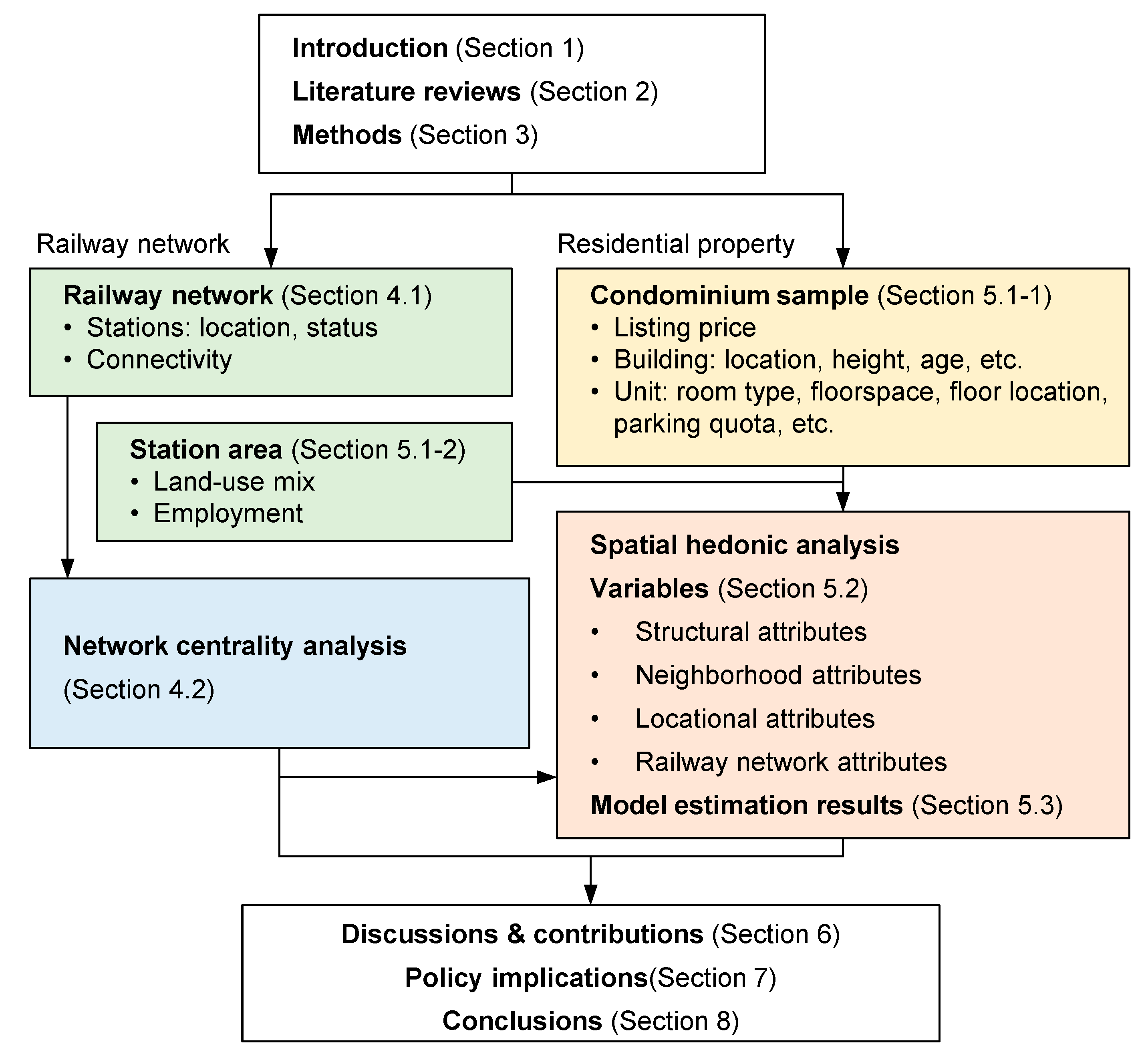
Figure 2.
Urban railway network in the Bangkok metropolitan region as of 2021.

Figure 3.
Evolution of Bangkok’s railway network centrality: (a) closeness centrality 2016, (b) betweenness centrality 2016, (c) closeness centrality 2021, (d) betweenness centrality 2021, (e) closeness centrality 2026, (f) betweenness centrality 2026, (g) degree centrality 2026, (h) eigenvector centrality 2026. Text in gray represents the corresponding railway line names, while the text in blue indicates the station names.
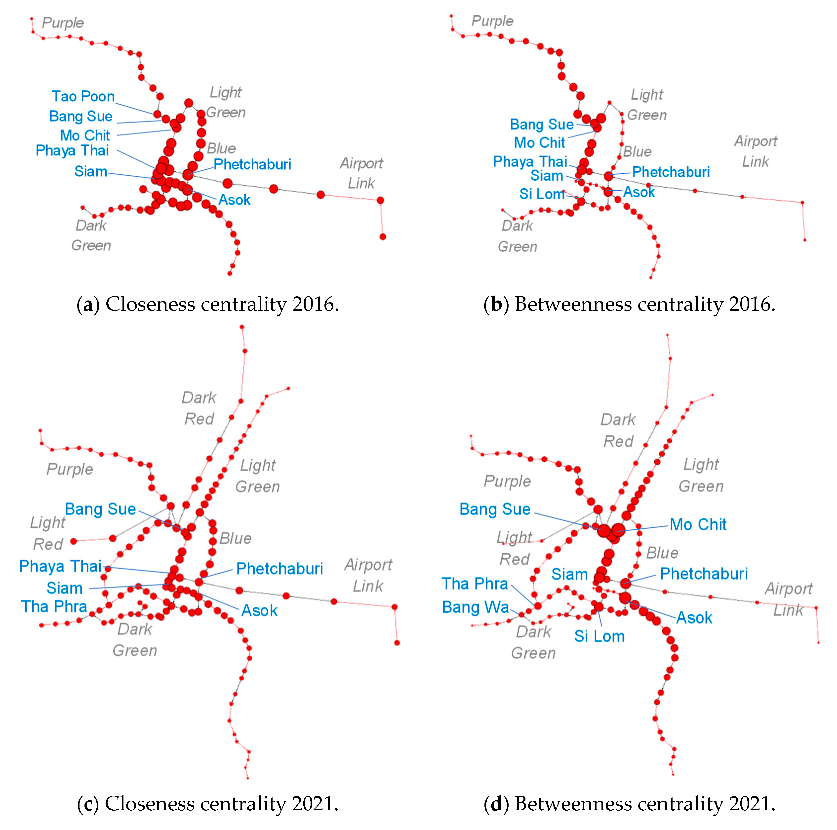
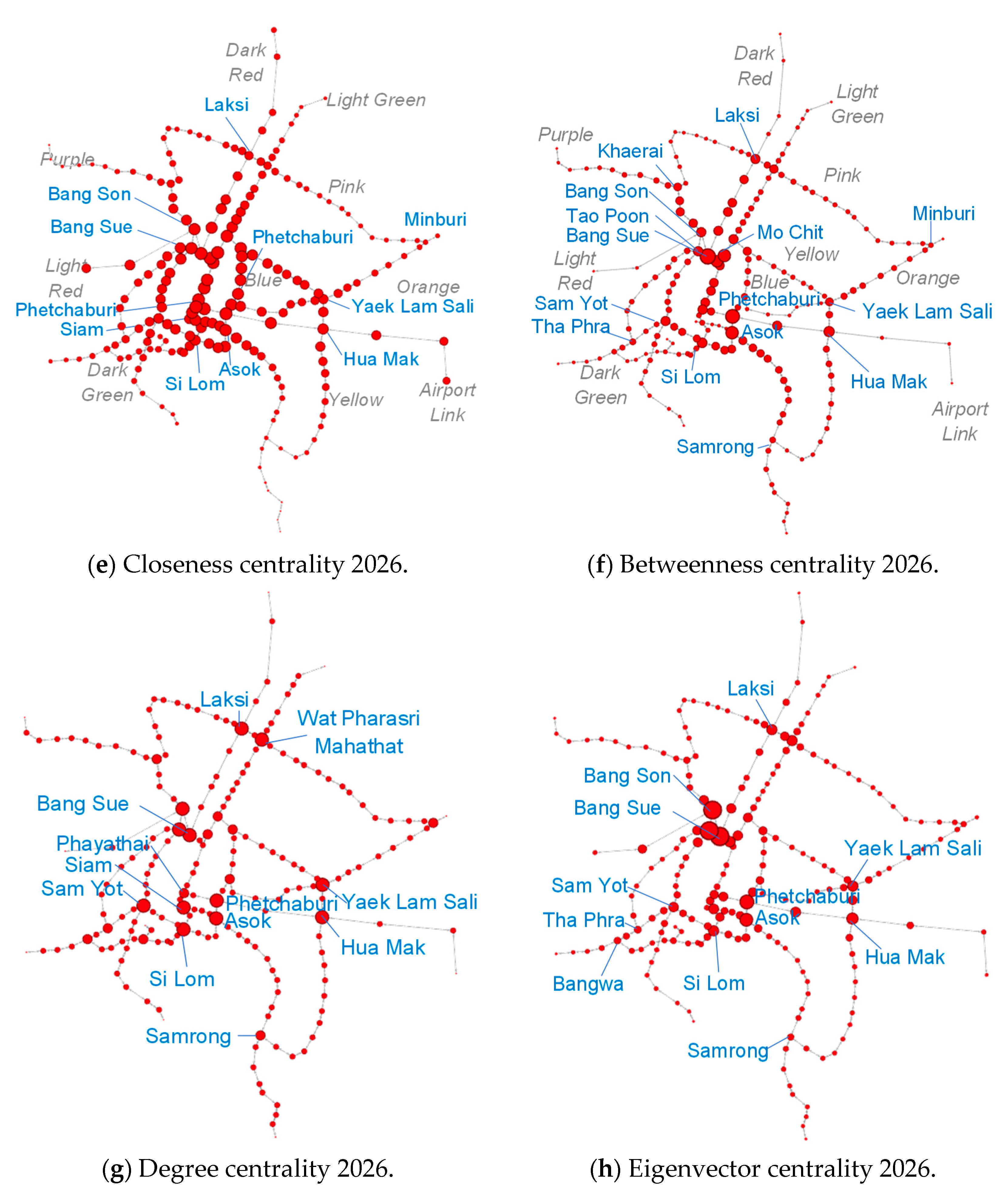
Figure 4.
The average listing price per square meter of the sample condominiums.
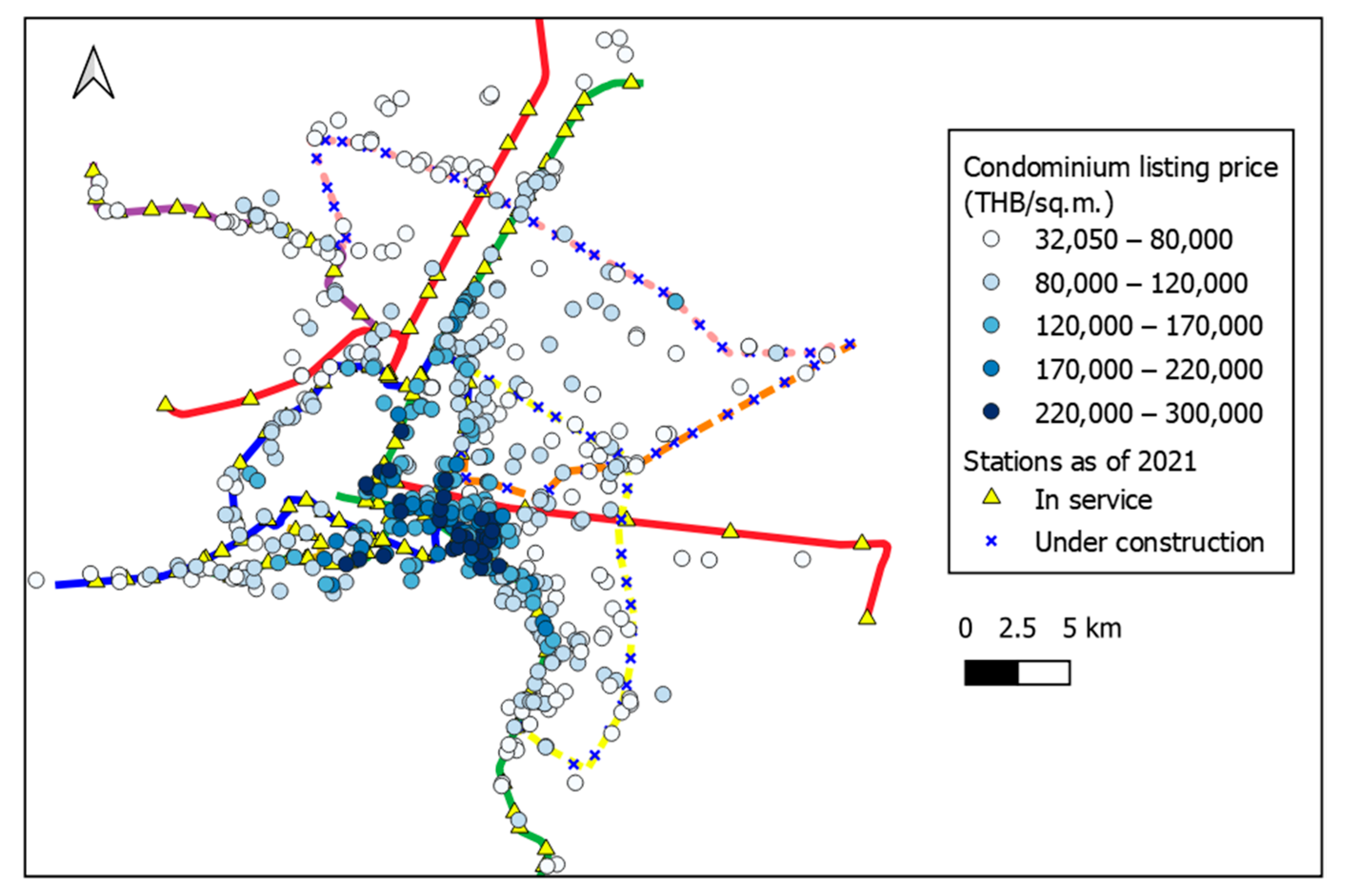
Figure 5.
Condominium prices per unit floorspace at varying distances measured along the path from railway stations.
Figure 5.
Condominium prices per unit floorspace at varying distances measured along the path from railway stations.
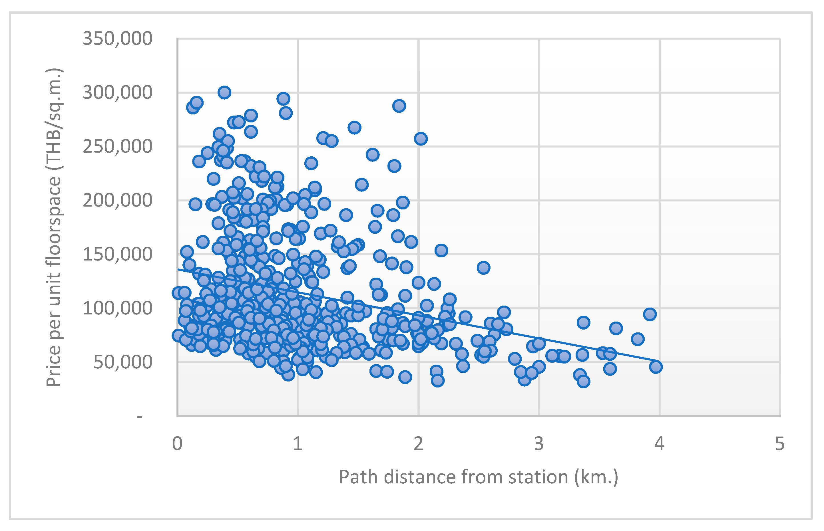

Table 1.
Summary statistics of the data used in the hedonic analysis (n = 505).
| Items (Unit) | Variables | Mean | std.dev. | min. | max. |
|---|---|---|---|---|---|
| Property value | |||||
| Listing price (Thai Baht) | - | 4,880,241 | 3,722,865 | 899,000 | 21,500,000 |
| Listing price per unit floorspace (Thai Baht per sq.m.) | PriceSqm | 113,199 | 56,752 | 32,050 | 300,0000 |
| Structural characteristics | |||||
| Floorspace of the unit (square meter) | Area | 40.81 | 18.53 | 21.70 | 224.00 |
| Age of the building (month) | Age | 25.11 | 28.20 | 0.05 | 248.00 |
| Category of the building (1 if high-rise, 0 otherwise) | HighRise | 0.49 | 0.50 | 0.00 | 1.00 |
| Neighborhood characteristics | |||||
| Land use mix index | LUM | 0.54 | 0.12 | 0.12 | 0.82 |
| Number of jobs around the station (persons) | Emp | 10,576.06 | 14,535.62 | 236.54 | 68,327.34 |
| Locational characteristics | |||||
| Euclidean distance to CBD: Siam Station (km.) | DistCBD | 9.57 | 5.20 | 0.77 | 26.38 |
| Euclidean distance to the nearest shopping mall (km.) | DistMall | 1.20 | 0.91 | 0.02 | 8.58 |
| Euclidean distance to the nearest hospital (km.) | DistHosp | 2.40 | 1.86 | 0.07 | 10.91 |
| Euclidean distance to the nearest university (km.) | DistUniv | 3.62 | 2.64 | 0.09 | 15.21 |
| Railway-related characteristics | |||||
| Proximity to the nearest station (Euclidean distance, km.) | - | 0.70 | 0.56 | 0.01 | 2.95 |
| Proximity to the nearest station (path distance, km.) | DistStn | 1.07 | 0.76 | 0.01 | 3.97 |
| Station status as of 2021 (1 if operational, 0 otherwise) | Open | 0.77 | 0.42 | 0.00 | 1.00 |
| Degree centrality of the nearest station in 2026 | CD | 4.25 | 0.91 | 2.00 | 8.00 |
| Closeness centrality of the nearest station in 2026 | CC | 0.070 | 0.013 | 0.038 | 0.091 |
| Betweenness centrality of the nearest station in 2026 | CB | 0.086 | 0.578 | 0.000 | 0.307 |
| Eigenvalue centrality of the nearest station in 2026 | CE | 0.126 | 0.121 | 0.010 | 0.978 |
Remark: as of September 2021, 1 USD (US Dollar) was approximately 33.34 THB (Thai Baht).
Table 2.
Estimation results of the five ordinary least square (OLS) models: (1) OLS as a base model, (2) OLS model with degree centrality, (3) OLS model with closeness centrality, (4) OLS model with betweenness centrality, and (5) OLS model with eigenvector centrality.
Table 2.
Estimation results of the five ordinary least square (OLS) models: (1) OLS as a base model, (2) OLS model with degree centrality, (3) OLS model with closeness centrality, (4) OLS model with betweenness centrality, and (5) OLS model with eigenvector centrality.
| Variables | Model 1 OLS | Model 2 OLS, Degree | Model 3 OLS, Closeness | Model 4 OLS, Betweenness | Model 5 OLS, Eigenvector | |||||
|---|---|---|---|---|---|---|---|---|---|---|
| Coeff. | t-Value | Coeff. | t-Value | Coeff. | t-Value | Coeff. | t-Value | Coeff. | t-Value | |
| Constant | 140,017.00 | *** 17.85 | 131,341.00 | *** 15.50 | 109,412.00 | *** 11.13 | 122,169.00 | *** 14.03 | 131,341.00 | *** 15.50 |
| Highrise | 12,678.20 | *** 3.21 | 11,387.70 | *** 2.87 | 11,017.90 | *** 2.84 | 11,781.70 | *** 3.03 | 11,387.70 | *** 2.87 |
| Area | 388.21 | *** 3.51 | 383.53 | *** 3.48 | 337.76 | *** 3.11 | 349.07 | *** 3.20 | 383.53 | *** 3.48 |
| Age | −394.13 | *** −5.71 | −397.83 | *** −5.79 | −387.74 | *** −5.74 | −384.28 | *** −5.66 | −397.83 | *** −5.79 |
| Emp | 1.05 | *** 6.70 | 1.07 | *** 6.82 | 1.05 | *** 6.85 | 1.11 | *** 7.16 | 1.07 | *** 6.82 |
| DistCBD | −3455.70 | *** −6.91 | −2957.60 | *** −5.56 | −2067.45 | *** −3.68 | −2623.51 | *** −4.99 | −2957.60 | *** −5.56 |
| DistHosp | −4067.75 | *** −3.51 | −4126.14 | *** −3.58 | −4688.96 | *** −4.12 | −4018.04 | *** −3.53 | −4126.14 | *** −3.58 |
| DistStation | −7855.79 | *** −3.01 | −7511.80 | *** −2.89 | −6030.39 | ** −2.34 | −7009.28 | *** −2.73 | −7511.80 | *** −2.89 |
| Open × CD | 42,699.10 | *** 2.62 | ||||||||
| Open × CC | 357,805.00 | *** 4.97 | ||||||||
| Open × CB | 138,321.00 | *** 4.39 | ||||||||
| Open × CE | 42,699.10 | *** 2.62 | ||||||||
| Adj. R-squared | 0.519 | 0.525 | 0.541 | 0.536 | 0.525 | |||||
| AIC | 12,153.3 | 12,148.4 | 12,130.8 | 12,136.1 | 12,148.4 | |||||
*** and ** indicate the significant levels of 0.01 and 0.05, respectively.
Table 3.
Estimation results of four spatial regression models: (6) spatial lag model with closeness centrality, (7) spatial lag model with betweenness centrality, (8) spatial error model with closeness centrality, and (9) spatial error model with betweenness centrality.
Table 3.
Estimation results of four spatial regression models: (6) spatial lag model with closeness centrality, (7) spatial lag model with betweenness centrality, (8) spatial error model with closeness centrality, and (9) spatial error model with betweenness centrality.
| Variables | Model 6 Lag, Closeness | Model 7 Lag, Betweenness | Model 8 Error, Closeness | Model 9 Error, Betweenness | ||||
|---|---|---|---|---|---|---|---|---|
| Coeff. | z-Value | Coeff. | z-Value | Coeff. | z-Value | Coeff. | z-Value | |
| Constant | 1414.05 | 0.12 | 10,821.70 | 0.94 | 135,476.00 | *** 7.76 | 149,275.00 | *** 8.74 |
| Highrise | 13,464.30 | *** 4.01 | 14,066.10 | *** 4.18 | 15,630.20 | *** 4.65 | 16,194.30 | *** 4.81 |
| Area | 244.29 | *** 2.60 | 256.47 | *** 2.72 | 209.77 | ** 2.24 | 224.18 | ** 2.39 |
| Age | −340.43 | *** −5.83 | −339.72 | *** −5.78 | −316.10 | *** −5.47 | −324.72 | *** −5.60 |
| Emp | 0.49 | *** 3.70 | 0.51 | *** 3.81 | 0.45 | ** 2.54 | 0.46 | *** 2.61 |
| DistCBD | 1063.61 | ** 1.98 | 632.85 | 1.19 | −3408.93 | *** −2.69 | −4296.76 | *** −3.45 |
| DistHosp | −2439.31 | ** −2.42 | −2047.19 | ** −2.05 | −3764.51 | ** −2.21 | −2758.86 | * −1.66 |
| DistStation | −7422.11 | *** −3.33 | −8130.73 | *** −3.65 | −8151.90 | *** −3.49 | −8510.20 | *** −3.64 |
| Open × CC | 205,621.00 | *** 3.27 | 199,132.00 | ** 2.47 | ||||
| Open × CB | 56,372.60 | ** 2.07 | 26,776.40 | 0.85 | ||||
| 0.785 | *** 14.90 | 0.791 | *** 15.04 | |||||
| 0.834 | *** 17.24 | 0.844 | *** 18.22 | |||||
| R-squared | 0.656 | 0.652 | 0.660 | 0.657 | ||||
| AIC | 12,012.6 | 12,019.1 | 12,008.6 | 12,013.9 | ||||
***, **, and * indicate the significance level of 0.01, 0.05 and 0.10, respectively.
Disclaimer/Publisher’s Note: The statements, opinions and data contained in all publications are solely those of the individual author(s) and contributor(s) and not of MDPI and/or the editor(s). MDPI and/or the editor(s) disclaim responsibility for any injury to people or property resulting from any ideas, methods, instructions or products referred to in the content. |
© 2023 by the authors. Licensee MDPI, Basel, Switzerland. This article is an open access article distributed under the terms and conditions of the Creative Commons Attribution (CC BY) license (https://creativecommons.org/licenses/by/4.0/).
Share and Cite
MDPI and ACS Style
Vichiensan, V.; Wasuntarasook, V.; Prakayaphun, T.; Kii, M.; Hayashi, Y. Influence of Urban Railway Network Centrality on Residential Property Values in Bangkok. Sustainability 2023, 15, 16013. https://doi.org/10.3390/su152216013
AMA Style
Vichiensan V, Wasuntarasook V, Prakayaphun T, Kii M, Hayashi Y. Influence of Urban Railway Network Centrality on Residential Property Values in Bangkok. Sustainability. 2023; 15(22):16013. https://doi.org/10.3390/su152216013
Chicago/Turabian StyleVichiensan, Varameth, Vasinee Wasuntarasook, Titipakorn Prakayaphun, Masanobu Kii, and Yoshitsugu Hayashi. 2023. "Influence of Urban Railway Network Centrality on Residential Property Values in Bangkok" Sustainability 15, no. 22: 16013. https://doi.org/10.3390/su152216013
Note that from the first issue of 2016, this journal uses article numbers instead of page numbers. See further details here.