
Spatiotemporal Changes in the Supply and Demand of Ecosystem Services in the Kaidu-Kongque River Basin, China


1
College of Economics and Management, Xinjiang Agricultural University, Urumqi 830052, China
2
College of Forestry and Landscape Architecture, Xinjiang Agricultural University, Urumqi 830052, China
3
State Key Laboratory of Desert and Oasis Ecology, Xinjiang Institute of Ecology and Geography, Chinese Academy of Sciences, Urumqi 830011, China
4
Xinjiang Academy of Forestry Sciences, Urumqi 830018, China
*
Authors to whom correspondence should be addressed.
Sustainability 2023, 15(11), 8949; https://doi.org/10.3390/su15118949
Submission received: 17 March 2023
/
Revised: 27 May 2023
/
Accepted: 29 May 2023
/
Published: 1 June 2023
(This article belongs to the Section Environmental Sustainability and Applications)
Abstract
:The assessment of ecosystem service (ES) supply and demand is crucial for the sustainable development of dryland drainage basins. The natural ecosystems in the Kaidu-Kongque River Basin have experienced severe ecological degradation in recent years, and the ES supply and demand were contradicted due to water scarcity and excessive water utilization. In this paper, the supply–demand of five key ecosystem services were evaluated, and their spatial matching was also analyzed to provide total insights. The services assessed were food supply, water yield, carbon sequestration, habitat quality, and windbreak and sand fixation. We utilized various models, including InVEST, RWEQ, and GeoDa, to quantify and analyze the spatial and temporal patterns of ecosystem service supply and demand between 1990 and 2020. Our findings indicate that the supply and demand for all ecosystem services in the basin have increased over the last 30 years. However, the spatial distribution of supply and demand for each ecosystem service is not completely consistent. Except for windbreak and sand fixation, where supply exceeds demand, there is a spatial mismatch between supply and demand for each service. Furthermore, we observed a positive and synergistic correlation between the supply and demand of each ecosystem service, with water yield services being the dominant and limiting factor. The spatial correlation between the supply and demand of ecosystem services was dominated by “low supply—low demand”, “high supply—high demand” spatial matching, and “low supply—high demand” mismatch, which could explain the variation in water yield from upstream to downstream. Based on our findings, we recommend policies and recommendations for ecological conservation and sustainable development in the Kaidu-Kongque River Basin. The ES supply and demand will become more reliable by increasing water supplies in the middle and lower reaches of the basin. Our results provide illumination for the maintenance and sustainability of ecosystem services in arid regions.
1. Introduction
Ecosystem services (ESs) are critical components of human survival, providing environmental conditions and utilities that sustain socio-economic systems [1,2]. The supply and demand of ecosystem services represent a delicate balance between natural ecosystems and human societies [3,4]. This dynamic process involves the flow of goods and services from ecosystems to socio-economic systems, and the spatial patterns of supply and demand have become a critical area of research in recent years [5,6]. Human well-being is usually affected by ES supply–demand mismatches due to unsatisfied demand [4], and it is of great significance to study the relationship between ES supply and demand for understanding the interactions between ES and humans’ well-being. However, the overexploitation of soil and water resources in arid regions has led to the imbalanced spatial distribution of land, resource scarcity, and ecosystem degradation, posing significant threats to regional ecological security. Therefore, clarifying the relationship between supply and demand and matching their spatial and temporal characteristics is crucial for promoting integrated ecosystem management, natural resource allocation, and optimizing land distribution.
Research on ES supply and demand originated in the 1990s, and it focused on the ecological carrying capacity and the ES values [7,8]. Early studies aimed to define the concept of ES supply and demand and refine the research framework by evaluating the structure and function of ESs [9]. Since 2000, more studies were conducted from quantifying ES supply and demand [10,11], matching them across space and time [12,13], studying their trade-off and synergy relationships [14], and optimizing ES supply and demand patterns [15]. In order to analyze the spatio-temporal characteristics and evaluate the ES supply and demand matching status, many researchers have developed spatialized methods such as land use estimation, ecological process simulation, spatial overlay analysis, expert empirical discrimination, InVEST model, and ARIES model [16,17], and different ES indicators have also been proposed for ES supply and demand evaluations from different perspectives, such as food supply [18], land cover information [19], the Ecosystem Services Provision Index (ESPI) and the Land Development Index (LDI) [20], and non-commodity ES [21]. The impacts of ES supply–demand changes on the urbanization [22] and land ecological consolidation [23] were also analyzed and evaluated to identify their trade-offs and synergies. However, due to the data availability and the method’s limitations, relatively few studies have explored ES supply and demand matching [24], particularly in underdeveloped areas with fragile ecosystems. Moreover, few studies have analyzed the impacts of variability and diversity across different spatial scales on the balance between ES supply and demand.
The Kaidu-Kongque River Basin is a complex ecosystem with a diverse range of physical features, including mountains, grasslands, rivers, oases, lakes, wetlands, and deserts. In recent decades, land cover changes, such as the conversion of deserts into oases, have driven socio-economic development in the dryland basin. However, these changes have also led to ecological problems, such as grassland degradation and soil erosion. To address these issues, various ecological conservation policies have been implemented, such as mountain closure to grazing and the return of grazing to grass [25]. Nevertheless, reconciling the promotion of ecological conservation with the maintenance of the balance between ecosystem service supply and demand remains a significant challenge.
This paper aims to provide a comprehensive understanding of the ES supply and demand changes in the Kaidu-Kongque River Basin. Five ecological services, namely, food supply, water yield, carbon sequestration, habitat quality, and windbreak and sand fixation, were chosen to illustrate their spatial matching relations, so as to formulate a scientific and rational method for the payment for ecosystem services (PES) and ecological compensation. The specific objectives of this study are threefold: (1) to assess the spatial distribution of ecosystem service supply and demand; (2) to evaluate the relationship between ecosystem service supply and demand matching; and (3) to provide the corresponding measures for the maintenance of ecosystem services.
2. Study Area and Data
2.1. Study Area
The Kaidu-Kongque River Basin is a primary tributary of the Tarim River Basin, which is situated between 82°57′ E–90°39′ E and 40°25′ N–43°21′ N (Figure 1). The basin spans an area of 9.37 × 10⁴ km2 and is characterized by a diverse, arid ecosystem comprising glaciers, forests, grasslands, rivers, wetlands, lakes, farmlands, and deserts. The altitude in the basin varies from 643 to 4817 m and the terrain descends from northwest to southeast. The primary water yield area is located in the upstream mountainous region, and the main water consumption area is in the midstream oasis, while the downstream riparian desert usually faces water shortages. The study area has a temperate continental climate; the average annual precipitation is 155.6 m; the annual potential evaporation is 2038.7 mm; and the drought index ranges from 2.5 to 41.8 [26].
2.2. Conceptual Framework
The ecosystem’s structure and functions in the Kaidu-Kongque River Basin have experienced severe ecological degradation and deterioration in recent years [26]. The problems of water scarcity, uneven water distribution, and excessive utilization have led to supply–demand contradictions of water resources, and the increasing agricultural yields and urbanization do not match the low habitat quality and aggravating desertification [27]. In arid regions, water resources are essential for almost all ecosystems; therefore, five essential ecosystem services, including food supply, water yield, carbon sequestration, habitat quality, and windbreak and sand fixation, were selected to analyze their ES supply and demand, as well as their spatial relationships and trade-offs. The interactions between the ES supply and demand were analyzed through quantitative and spatial relations [28]. Specifically, surplus, balance, and deficit represent the quantitative relations, while matching, aggregation, and spatial coupling coordination represent the spatial relations, as shown in Figure 2. Moreover, spider diagrams and spatial autocorrelation models were also employed to explore the spatial correlations between the ES supply and demand, and their supply–demand mismatch in different spatial regions was also analyzed to reveal the inequality between the ES provision and social demands.
2.3. Data Collection
Various data sources were used to model and analyze the ecological supply and social demand during 1990–2020, as shown in Table 1. Specifically, crop yield, energy consumption, water consumption, and per capita food demand data were obtained from the Xinjiang Statistical Yearbook. The grid data sources, such as land use and land cover (LULC) map, DEM, soil map, and meteorological data, were combined to analyze the spatial patterns of the ecological services, and all these raster data sources were converted to the uniform projection system (WGS, 1984; UTM Zone 45 N), and the raster data grid was resampled to 1 km × 1 km.
3. Methods
3.1. Quantitative Assessment of the Supply and Demand of Ecosystem Services
To assess the supply and demand relationship of the ecosystem services in the Kaidu-Kongque River Basin, a multidimensional approach was proposed based on biophysical and social attributes [28]. The calculation methods used for the five ecosystem services are detailed in Table 2. To determine food production, we employed NDVI distribution to assign food production to grids, given the strong linear correlation between food production and NDVI [29,30]. The per capita grain demand was determined by population density and the per capita grain demand, which was derived from Xinjiang Statistical Yearbook [31]. Water yield, carbon sequestration, and habitat quality were modeled using the InVEST model, and windbreak and sand fixation were simulated using the modified wind erosion equation (RWEQ). The InVEST model (Integrate Valuation of Ecosystem Service and Trade-offs Tool) is a spatially explicit toolset that uses maps as information sources, produces maps as outputs, and integrates geo-information technology into ES evaluations at local, regional, or global scales. The InVEST model is based on production functions that define how changes in an ecosystem’s structure and function are likely to affect the ES values, and it returns results in either biophysical or economic terms.

Table 2.
Quantitative model of ES supply and demand.
| Types of ES | Calculation Method | Reference | ||
|---|---|---|---|---|
| Supply | Demand | The Meaning of Each Parameter | ||
| Food | Where is the yield of grain, meat, fruit, and aquatic products allocated by i grid; is the total grain output, meat, fruit, and aquatic products output in the study area. is the normalized vegetation index of grid i; is the sum of NDVI values in the study area. is the food requirement; is the per capita food demand; is the population size. | [2,29] | ||
| Water yield | Where denotes the annual water supply service on the raster cell, denotes the average annual evapotranspiration on the raster cell, and denotes the average annual precipitation on the raster cell. is the total water demand; is the amount of water used for agricultural irrigation; is the industrial water consumption; is water consumption for residential use; is the ecological water consumption; is water consumption for livestock. | [32,33,34] | ||
| Carbon sequestration | Where is total carbon stock (t·hm−2), is aboveground biogenic carbon (t·hm−2), is belowground biogenic carbon (t·hm−2), is soil organic carbon (t·hm−2), and is dead organic matter (t·hm−2). The carbon density data in the carbon pool table required for the model were mainly referred to in the relevant literature. E is energy consumption; GDP is gross domestic product; P is population size. | [34,35] | ||
| Habitat quality | Where is the degree of habitat degradation, ranging from 0 to 1, with higher values representing higher degrees of habitat degradation; is the threat factor; is the number of grids corresponding to the threat factor r; is the weight of the threat factor; is the stress value of the threat factor; is the level of habitat protection; is the sensitivity of habitat j to the threat factor r; is the influence of the threat factor r in grids y on grids x; is the average degree of demand for habitat quality services; is the degree of demand for biodiversity based on species POI data; is the degree of environmental demand for human habitat based on population density; is the degree of environmental demand for socio-economic development classified by the density of GDP distribution. | [35,36,37,38,39] | ||
| Windbreak and sand fixation | Where is sand fixation (t·hm−2), is the maximum sand transport capacity of potential wind (kg/m), is the potential critical plot length (m), z denotes the calculated downwind distance (m). A total of 50 m was taken for this calculation. is the maximum sand transport capacity of the actual wind (kg/m); sr is the actual critical plot length (m). | [40,41,42] | ||
3.2. Relationships among Ecosystem Services
3.2.1. Ecological Supply to Demand Ratio
To assess the relationship between ecosystem service supply and demand and reflect the coordinated development of ecosystem services, we utilized the ecosystem service supply and demand ratio (ESDR) [43]. The formula for calculating ESDR is as follows:
where and represent the supply and demand of the nth ecosystem service, respectively, while and denote the maximum supply and demand of the nth service in the study area. A positive ESDR indicates that supply exceeds demand. When ESDR > 0, supply exceeds demand; when ESDR = 0, the supply and demand of ecosystem services remain balanced; when ESDR < 0, supply exceeds demand [18,23].
3.2.2. Local Indicators of Spatial Associations
Local indicators of spatial associations (LISA) are used to measure the spatial clustering and attribute correlations between neighboring spatial units [2,18,44]. In the context of analyzing the spatial correspondence between ES supply and demand, LISA can be used to visualize the spatial matching patterns of each ES. The calculation formula for LISA is as follows:
where is the spatial weight matrix between units, is the attribute value of the unit, is the average value of all attribute values, and n denotes the total number of regional units. If LISA > 0, it indicates the spatial aggregation of supply and demand of spatial units, such as High—High (H—H) or Low—Low (L—L) values, and they show spatial units with high supply—high demand and low supply—low demand; respectively; while if LISA < 0, it indicates the spatial aggregation of High–Low (H—L) or Low—High (L—H) values.
4. Results
4.1. Spatio-Temporal Dynamics of Supply, Demand, and Supply–Demand Ratio
Using the InVEST model and ArcGIS, we analyzed the changes in the supply, demand, and supply–demand ratio of the five ecosystem services at the basin and county scales during 1990–2020 (Figure 3, Figure 4 and Figure 5). Our findings reveal an overall increasing trend in the supply and demand of ecosystem services in the Kaidu-Kongque River Basin during this period. Specifically, the food supply increased by 197.32%, from 26.52 kg/hm2 to 78.85 kg/hm2, while the water yield increased by 27.16%, from 440.45 m3/hm2 to 560.09 m3/hm2. Carbon sequestration increased from 4.34 kg/hm2 to 4.78 kg/hm2; habitat quality increased from 0.44 to 0.57; and windbreak and sand fixation increased from 1.51 kg/m2 to 4.18 kg/m2. The demand for food supply, water production, carbon sequestration, habitat quality, and windbreak and sand fixation increased by 57.80%, 56.57%, 1135.29%, 25.0%, and 261.4%, respectively. Notably, the increase was significant during 2000–2010, while it slowed down after 2010.
From the perspective of spatial patterns, the supply and demand of ESs showed various spatial distributions across different sub-regions of the Kaidu-Kongque River Basin. In terms of ES supplies (Figure 3), the water yield supply is mainly clustered around the upstream mountainous regions, where glaciers and precipitation contribute most of the available water resources in the whole basin. The carbon sequestration and the habitat quality supply were concentrated in areas with high vegetation cover, such as the upstream grasslands and the midstream cultivated areas, while the food supply was only higher in the cultivated areas, such as the Yanqi County, the Korla City, and the Yuli County. Especially, the food supply ES in Yuli County has increased remarkably during the last 30 years with the arable land expansion. The windbreak and sand fixation supply has increased quickly in the upstream alpine meadow grasslands since 2000, indicating that the rangeland degradation is serious, and this trend was also obvious in the downstream desert riparian forests.
In terms of ES demands (Figure 4), both the food and carbon sequestration services had slight increases in the densely populated areas, such as Korla City and Yuli County, where population growth was rising rapidly since 2000. Therefore, the water ES demand was larger in these areas due to the population increase. The habitat quality ES demand was increasing in both populations with increasing and reclamation areas, especially in Korla City and Yuli County. However, the windbreak and sand fixation ES demand increased remarkably throughout the basin, and this trend was obvious after 2010, especially in the vegetation degradation regions, and this means that ecosystem degradation was obvious not only in the mountainous rangelands and desert riparian zones but also in populated areas in the midstream.
Moreover, in order to analyze the spatio-temporal changes in the five ESs during 1990–2020 (Figure 5), the ESDRs were also applied to describe the pattern changes more clearly. The ESDR of food supply and water yield increased steadily in the upstream but decreased rapidly in the midstream populated areas, which means that the demands exceeded the supplies with the increasing cultivated lands and population. The ESDRs of carbon sequestration decreased in the newly cultivated lands after 2000, while those of windbreak and sand fixation decreased throughout the upstream and midstream areas, which means that the ecosystems became more fragile and the ecological function began decreasing.
4.2. Quantitative Relations between Supplies and Demands
In order to evaluate the quantitative relations between ES supplies and demands, the ESDRs were also counted by both administrative divisions and the whole basin (Table 3). At the basin scale, the supplies of food supply, water yield, carbon sequestration, and habitat quality ESs were larger than the ES demands over the last 30 years, while the windbreak and sand fixation ES is an exception to this. However, if these relations were counted by administrative divisions, the ESDRs of food supply, carbon sequestration, and habitat quality had the same pattern as those by the whole basin, while the ESDRs of water yield had different spatial patterns. Hejing County is located upstream of the basin, which contributes most water resources of the basin, and the positive ESDR value means that the water supply is sufficient, while the other counties and Korla City are faced with water shortages. The windbreak and sand fixation ES has negative ESDR values in both administrative divisions and the whole basin, which means that its supply cannot meet its demand. Additionally, it is also shown in the ES supply and demand structure map (Figure 6a,b), where the windbreak and sand fixation ESs improved a lot due to the increase in ES supplies. The reason for this trend may be the result of ecological environment protection policies and population increase in the study area [20,25].
4.3. Spatial Characterization of Ecosystem Service Mismatches
In order to analyze the spatial matching relationship between the supply and demand of ecosystem services in the Kaidu-Kongque River Basin from 1990 to 2020, the Bivariate Local Moran’s I was calculated to produce the LISA cluster diagram (Figure 7) to measure the spatial differences under various conditions of excessive ES supplies or unsatisfied ES demands. The results indicated that the water yield ES had a negative correlation between supplies and demands, while the other four ESs had positive correlations. The areas with high supply–high demand (H–L) mode and low supply–high demand (L–H) mode are mainly located around densely populated areas such as Yanqi Basin and Korla City in the midstream of the drainage basin. Additionally, there is also a large amount of bare and unused land in the study area, with the characteristic of low supply– low demand.
Over the period of 1990–2020, the ES low supply–high demand (L–H) mismatch relations shown a trend of firstly increasing and then decreasing changes, and this trend was significant during 2000–2010. The area percentages of L–H mismatches for food supply, water production, carbon sequestration, and habitat quality, and windbreak and sand fixation ESs accounted for 0.14%, 9.43%, 1.92%, 3.2%, and 12.63%, respectively. Moreover, the L–H mismatches for food supply, water production, carbon sequestration, habitat quality ESs were mainly distributed in densely populated cities and cultivated areas, while the windbreak and sand fixation ES was primarily distributed in the upstream grassland degradation area and the downstream desert riparian zones.
5. Discussion
5.1. Assessment of ES Supply and Demand
The ES supplies and demands in the Kaidu-Kongque River Basin are severely influenced by the local climatic and hydrothermal conditions, as well as land use types, population, and the level of socioeconomic development [22]. The spatial mismatches reflected an imbalance between demand and supply (see Table 3 and Figure 6). Specifically, the food, water, carbon sequestration, and habitat quality ecosystem services provided more supplies than demands, while the opposite is true for the windbreak and sand fixation services [45,46]. Moreover, high-supply areas are mainly located in the upstream areas, where water supplies are sufficient with plenty of precipitation and glacial melt water, while high-demand areas are usually located in the midstream, densely populated areas, where water demands increase dramatically due to land reclamation and urbanization [42] (see Figure 5). It is essential to make effective management and conservation strategies to ensure the sustainability of ecosystem services across the basin, especially for windbreak and sand fixation services [47].
The ES supply–demand relationship highlights the dependence of society on specific ecosystem services and the impact of social needs on their supply [48]. The spatial pattern between ES supply and demand is influenced by various factors, including natural, social, economic, and technical factors [49]. Firstly, the midstream oases have low water supplies but high water demands, leading to a significant spatial mismatch in densely population areas and newly cultivated land areas. Secondly, as the land cover types have changed dramatically in recent years due to urbanization and reclamation, the spatial mismatching areas of ES supply demands are largely related to areas with significant land surface changes, resulting in the obvious spatial heterogeneity of ecosystem services. Thirdly, water scarcity is common in arid regions, and the uneven distribution of water resources aggravates the degree of water supply. The midstream oases and downstream desert areas have insufficient water supply services, and the carbon sequestration and habitat quality supplies and demands also have different spatial mismatches in the low supply–high demand (L–H) and high supply–low demand (H–L) areas. Water-saving irrigation technology and ecological water transfer have been applied to alleviate the water supplies, such as the ecological water transferring project in the downstream of Kongque River (see Figure 7), which has proven to be beneficial to the ecological restoration of the desert riparian forests [50]. Therefore, more water supplies are suggested to transfer to the midstream and downstream to provide sustainable ecosystem services and coordinate the supply–demand of natural ecosystem services in the Kaidu-Kongque River Basin.
5.2. Future Outlook and Policy Recommendations
In order to address the spatial mismatches of ES supplies and demands, many measures have been taken to improve the balance of supplies and demands. Specifically, water-saving irrigation technologies in arid areas should be promoted, and ecological water transfer projects can be utilized to alleviate water shortages. To address food mismatches, road networks are improved for the mobility of agricultural products in the middle and upper reaches. Furthermore, in order to improve the sand fixation balance between supply and demand, ecological conversation policies, such as afforestation, and Grain for Green, are necessary. These efforts will help to mitigate the mismatch between supply and demand and promote the sustainable management of ecosystem services.
The recent implementation of the “three zones and three lines” policy by the Chinese government is expected to address these spatial mismatches to some extent. In terms of windbreak and sand fixation services, our findings suggest that the demand for these services is concentrated in areas that coincide with supply areas, but the supply is still inadequate. Despite the fact that the northwest region is primarily covered with grassland, we observed a surge in demand for these services. This can be attributed to the rapid expansion of animal husbandry, leading to grassland degradation and desertification, and the amplified impact of wind erosion due to locally strong winds [46]. As a result, the gap between supply and demand for this service is projected to widen between 1990 and 2020 as vegetation coverage in the northwestern part of the study area decreases and wind speeds generally increase throughout the region [41].
5.3. Limitations and Future Directions
The ES supply and demand changes and their correlations were effectively incorporated into ecological conservation and policymaking. However, the study has the following limitations: Firstly, some indicators for ES calculations, such as the GDP, population, and nighttime light data, were similar when representing anthropogenic indicators, and more factors, such as eco-environmental and socio-economic factors, should be involved in ES calculations for accurately characterizing ES supply and demand. Secondly, ES supply and demand are dynamic processes that may change over time, but this study simplified the ES changes only in 1990, 2000, 2010, and 2020, and more detailed data with shorter time spans will be employed to capture these changes accurately. Thirdly, ES supply and demand varies with regions and social-ecological backgrounds, so the impact factors and the relations between ES supply and demand changes will also be emphasized to analyze its mechanism in future study.
6. Conclusions
As one of the nine tributaries of the Tarim River, the Kaidu-Kongque River plays an irreplaceable role in water resource management and ecosystem services. In this study, the InVEST model, RWEQ model, and ArcGIS spatial analysis tool were employed to evaluate the supply and demand of five key ESs based on multi-source data, and the ES supply and demand were also analyzed to provide insights into their spatial matching. The conclusion is as follows:
- (1)
- Generally, the ES supply and demand showed an overall increased trend from 1990 to 2020, and the food supply, water production, carbon sequestration, and habitat quality services showed an increasing trend, which means that the supply exceeded the actual demands, while the windbreak and sand fixation service showed a decreasing trend, indicating a rising need for this service.
- (2)
- The spatial heterogeneity of ES supplies and demand varied over time. High-supply areas are mainly located in the upstream natural and rural areas, while high-demand areas are usually located in the midstream densely populated areas and downstream riparian desert zones. These ES mismatches indicated the imbalance between ES supply and demand.
- (3)
- Although the overall water yield was relatively sufficient at the basin scale, the water supply varied across the different regions. The upstream mountainous area was sufficient in water supply, while the midstream oases and downstream riparian zones were insufficient in water supply, which makes low supply–high demand mismatches for food supply, water yield, carbon sequestration, and habitat quality services, which were mainly distributed in densely populated cities and cultivated areas. The optimization of water supply in the midstream and downstream is suggested to provide sustainable ecosystem services and coordinate the supply–demand of natural ecosystem services.
In this study, the ES supply and demand changes and their correlations were effectively incorporated into ecological conservation and policymaking. In order to gain a more thorough understanding, more social and ecological factors will be used for accurate ES calculations, and more detailed changes on temporal scales should be extended in the future.
Author Contributions
Conceptualization, methodology, software, writing—original draft preparation, visualization: J.L. (Jiangui Li) and J.L. (Junli Li); validation, formal analysis, data curation: J.L. (Junli Li); writing—review and editing: Y.Y.; supervision, project administration, funding acquisition, T.J. All authors have read and agreed to the published version of the manuscript.
Funding
This research was funded by the Tianshan Talent-Science and Technology Innovation Team, No. 2022TSYCTD0006, the National Natural Science Foundation of China, No. U203201, and the Third Integrated Scientific Expedition Project in Xinjiang, No. 2021xjkk1403, who we thank for their support of this research.
Institutional Review Board Statement
Not applicable.
Informed Consent Statement
Not applicable.
Data Availability Statement
Not applicable.
Acknowledgments
The data that support the findings of this study are available on request from the corresponding author. The data are not publicly available due to privacy or ethical restrictions. Thanks to L Z for his comments on the revision of the manuscript.
Conflicts of Interest
The authors declare no conflict of interest.
References
- Wolff, S.; Schulp, C.J.E.; Verburg, P.H. Mapping ecosystem services demand: A review of current research and future perspectives. Ecol. Indic. 2015, 55, 159–171. [Google Scholar] [CrossRef]
- Liu, L.C.; Liu, C.F.; Wang, C.; Li, P. Supply and demand matching of ecosystem services in loess hilly region: A case study of Lanzhou. Prog. Chem. 2019, 74, 1921–1937. [Google Scholar]
- Mathieu, L.; Tinch, R.; Provins, A. Catchment management in England and Wales: The role of arguments for ecosystems and their services. Biodivers. Conserv. 2018, 27, 1639–1658. [Google Scholar] [CrossRef]
- Wei, H.; Fan, W.; Wang, X.; Lu, N.; Dong, X.; Zhao, Y.; Ya, X.; Zhao, Y. Integrating supply and social demand in ecosystem services assessment: A review. Ecosyst. Serv. 2017, 25, 15–27. [Google Scholar] [CrossRef]
- Burkhard, B.; Maes, J. Mapping ecosystem services. Adv. Books 2017, 1, e12837. [Google Scholar]
- Schirpke, U.; Candiago, S.; Vigl, L.E.; Jäger, H.; Labadini, A.; Marsoner, T.; Meisch, C.; Tasser, E.; Tappeiner, U. Integrating supply, flow and demand to enhance the understanding of interactions among multiple ecosystem services. Sci. Total Environ. 2019, 651, 928–941. [Google Scholar] [CrossRef]
- Rees, W.E. Ecological footprints and appropriated carrying capacity: What urban economics leaves out. Environ. Urban. 1992, 4, 121–130. [Google Scholar] [CrossRef]
- Tiemann, A.; Ring, I. Towards ecosystem service assessment: Developing biophysical indicators for forest ecosystem services. Ecol. Indic. 2022, 137, 108704. [Google Scholar] [CrossRef]
- Başak, E.; Cetin, N.I.; Vatandaşlar, C.; Pamukcu-Albers, P.; Karabulut, A.A.; Çağlayan, S.D.; Besen, T.; Erpul, G.; Balkız, Ö.; Çokçalışkan, B.A.; et al. Ecosystem services studies in Turkey: A national-scale review. Sci. Total Environ. 2022, 844, 157068. [Google Scholar] [CrossRef]
- Schulp, C.J.E.; Lautenbach, S.; Verburg, P.H. Quantifying and mapping ecosystem services: Demand and supply of pollination in the European Union. Ecol. Indic. 2014, 36, 131–141. [Google Scholar] [CrossRef]
- Sauter, I.; Kienast, F.; Bolliger, J.; Winter, B.; Pazúr, R. Changes in demand and supply of ecosystem services under scenarios of future land use in Vorarlberg, Austria. J. Mt. Sci. 2019, 16, 2793–2809. [Google Scholar] [CrossRef]
- Lorilla, R.S.; Kalogirou, S.; Poirazidis, K.; Kefalas, G. Identifying spatial mismatches between the supply and demand of ecosystem services to achieve a sustainable management regime in the Ionian Islands (Western Greece). Land Use Policy 2019, 88, 104171. [Google Scholar] [CrossRef]
- Roces-Díaz, J.V.; Vayreda, J.; Banqué-Casanovas, M.; Díaz-Varela, E.; Bonet, J.A.; Brotons, L.; de-Miguel, S.; Herrando, S.; Martínez-Vilalta, J. The spatial level of analysis affects the patterns of forest ecosystem services supply and their relationships. Sci. Total Environ. 2018, 626, 1270–1283. [Google Scholar] [CrossRef]
- Liu, C.F.; Wang, W.T.; Liu, L.C.; Li, P.-J. Supply-demand matching of county ecosystem services in Northwest China: A case study of Gulang county. J. Nat. Resour. 2020, 35, 2177–2190. [Google Scholar] [CrossRef]
- Schirpke, U.; Meisch, C.; Marsoner, T.; Tappeiner, U. Revealing spatial and temporal patterns of outdoor recreation in the European Alps and their surroundings. Ecosyst. Serv. 2018, 31, 336–350. [Google Scholar] [CrossRef]
- Larondelle, N.; Lauf, S. Balancing demand and supply of multiple urban ecosystem services on different spatial scales. Ecosyst. Serv. 2016, 22, 18–31. [Google Scholar] [CrossRef]
- Syrbe, R.U.; Grunewald, K. Ecosystem service supply and demand—The challenge to balance spatial mismatches. Int. J. Biodivers. Sci. Ecosyst. Serv. Manag. 2017, 13, 148–161. [Google Scholar] [CrossRef]
- Ala-Hulkko, T.; Kotavaara, O.; Alahuhta, J.; Hjort, J. Mapping supply and demand of a provisioning ecosystem service across Europe. Ecol. Indic. 2019, 103, 520–529. [Google Scholar] [CrossRef]
- Burkhard, B.; Kroll, F.; Nedkov, S.; Müller, F. Mapping ecosystem service supply, demand and budgets. Ecol. Indic. 2012, 21, 17–29. [Google Scholar] [CrossRef]
- Wang, J.; Zhai, T.; Lin, Y.; Kong, X.; He, T. Spatial imbalance and changes in supply and demand of ecosystem services in China. Sci. Total Environ. 2019, 657, 781–791. [Google Scholar] [CrossRef]
- Wolff, S.; Schulp, C.J.E.; Kastner, T.; Verburg, P. Quantifying spatial variation in ecosystem services demand: A global mapping approach. Ecol. Econ. 2017, 136, 14–29. [Google Scholar] [CrossRef]
- Peng, J.; Wang, X.; Liu, Y.; Zhao, Y.; Xu, Z.; Zhao, M.; Qiu, S.; Wu, J. Urbanization impact on the supply-demand budget of ecosystem services: Decoupling analysis. Ecosyst. Serv. 2020, 44, 101139. [Google Scholar] [CrossRef]
- Xie, Y.; Zhang, S.; Lin, B.; Zhao, Y.; Hu, B. Spatial zoning for land ecological consolidation in Guangxi based on the ecosystem services supply and demand. J. Nat. Resour. 2020, 35, 217–229. [Google Scholar]
- Qian, C.Y.; Gong, J.; Zhang, J.; Liu, D.; Ma, X.C. Change and tradeoffs-synergies analysis on watershed ecosystem services: A case study of Bailongjiang Watershed, Gansu. Acta Geogr. Sin. 2018, 73, 868–879. [Google Scholar]
- Li, Q.; Pu, C.; Liu, P.; Wei, Z.; Liu, C. A Survey on policy of transforming grazing lands to pastures and its influential factors interviewed with herdsmen in Xinjiang Uygur Autonomous Region. Bull. Soil Water Conserv. 2015, 35, 281–284. [Google Scholar]
- Chen, Y.; Du, Q.; Chen, Y. Sustainable Utilization of Water Resources in Bosten Lake Basin; Science Press: Beijing, China, 2013; pp. 1–25. [Google Scholar]
- Maco, B.; Bardos, P.; Coulon, F.; Erickson-Mulanax, E.; Hansen, L.J.; Harclerode, M.; Hou, D.; Mielbrecht, E.; Wainwright, H.M.; Yasutaka, T.; et al. Resilient remediation: Addressing extreme weather and climate change, creating community value. Remediat. J. 2018, 29, 7–18. [Google Scholar] [CrossRef]
- Villamagna, A.M.; Angermeier, P.L.; Bennett, E.M. Capacity, pressure, demand, and flow: A conceptual framework for analyzing ecosystem service provision and delivery. Ecol. Complex. 2013, 15, 114–121. [Google Scholar] [CrossRef]
- Chen, T.; Feng, Z.; Zhao, H.; Wu, K. Identification of ecosystem service bundles and driving factors in Beijing and its surrounding areas. Sci. Total Environ. 2020, 711, 134687. [Google Scholar] [CrossRef]
- Tucker, C.J. Red and photographic infrared linear combinations for monitoring vegetation. Remote Sens. Environ. 1979, 8, 127–150. [Google Scholar] [CrossRef]
- Cui, F.; Tang, H.; Zhang, Q.; Wang, B.; Dai, L. Integrating ecosystem services supply and demand into optimized management at different scales: A case study in Hulunbuir, China. Ecosyst. Serv. 2019, 39, 100984. [Google Scholar] [CrossRef]
- Zhan, T.; Yu, Y.; Wu, X. Supply-demand spatial matching of ecosystem services in the Huangshui River Basin. Acta Ecol. Sin. 2021, 41, 7260–7272. [Google Scholar]
- Palásti, P.; Gulyás, Á.; Kiss, M. Mapping Freshwater Aquaculture’s Diverse Ecosystem Services with Participatory Techniques: A Case Study from White Lake, Hungary. Sustainability 2022, 14, 16825. [Google Scholar] [CrossRef]
- Zhang, P.T.; Liu, S.J.; Zhou, Z.; Liu, C.; Xu, L.; Gao, X. Supply and demand measurement and spatio-temporal evolution of ecosystem services in Beijing-Tianjin-Hebei Region. Acta Ecol. Sin. 2021, 41, 3354–3367. [Google Scholar]
- Baró, F.; Haase, D.; Gómez-Baggethun, E.; Frantzeskaki, N. Mismatches between ecosystem services supply and demand in urban areas: A quantitative assessment in five European cities. Ecol. Indic. 2015, 55, 146–158. [Google Scholar] [CrossRef]
- Wang, Y.; Niu, M.; Song, B. Research on Supply and Demand of Habitat Maintenance Services: A Case Study of Beijing-Tianjin-Hebei Region. Acta Sci. Nat. Univ. Peking 2021, 57, 381–389. [Google Scholar]
- Liu, F.T.; Xu, E.Q. Comparison of spatial-temporal evolution of habitat quality between Xinjiang Corps and Non-corps Region based on land use. J. Appl. Ecol. 2020, 31, 2341–2351. [Google Scholar]
- Hao, L. Analysis of Ecological Security Pattern in Shanghai Based on the Supply Demand Relationship of Ecosystem Services. Master’s Thesis, Chang’an University, Xi’an, China, 2021. [Google Scholar]
- Yang, M.; Zhang, Y.; Wang, C. Spatial-temporal Variations in the Supply-demand Balance of Key Ecosystem Services in Hubei Province. Resour. Environ. Yangtze Basin. 2019, 28, 2080–2091. [Google Scholar]
- Xu, J.; Xiao, Y.; Xie, G.; Wang, Y.; Jiang, Y.; Chen, W. Assessment of wind erosion prevention service and its beneficiary areas identification of national key ecological function zone of windbreak and sand fixation type in China. Acta Ecol. Sin. 2019, 39, 5857–5873. [Google Scholar]
- Chen, J.; Jiang, B.; Bai, Y.; Xu, X.; Alatalo, J.M. Quantifying ecosystem services supply and demand shortfalls and mismatches for management optimisation. Sci. Total Environ. 2019, 650, 1426–1439. [Google Scholar] [CrossRef]
- Xu, M. Relationship between Supply and Demand of Ecosystem Services and Human Well-Being in the Arid Region of Northwest China. Master’s Thesis, China University of Geosciences (Beijing), Beijing, China, 2021. [Google Scholar]
- Shi, Y.S.; Shi, D.H. Study on the balance of ecological service supply and demand in Dongting Lake ecological economic zone. Geogr. Res. 2018, 37, 1714–1723. [Google Scholar]
- Anselin, L. Local indicators of spatial association—LISA. Geogr. Anal. 1995, 27, 93–115. [Google Scholar] [CrossRef]
- Martínez-Harms, M.J.; Balvanera, P. Methods for mapping ecosystem service supply: A review. Int. J. Biodivers. Sci. Ecosyst. Serv. Manag. 2012, 8, 17–25. [Google Scholar] [CrossRef]
- Zhang, Y.; Shi, X.; Tang, Q. Carbon storage assessment in the upper reaches of the Fenhe River under different land use scenarios. Acta Ecol. Sin. 2021, 41, 360–373. [Google Scholar]
- Lang, Y.; Song, W.; Zhang, Y. Responses of the water-yield ecosystem service to climate and land use change in Sancha River Basin, China. Phys. Chem. Earth 2017, 101, 102–111. [Google Scholar] [CrossRef]
- Lorilla, R.S.; Poirazidis, K.; Detsis, V.; Kalogirou, S.; Chalkias, C. Socio-ecological determinants of multiple ecosystem services on the Mediterranean landscapes of the Ionian Islands (Greece). Ecol. Model 2020, 422, 108994. [Google Scholar] [CrossRef]
- Keeler, B.L.; Hamel, P.; McPhearson, T.; Hamann, M.H.; Donahue, M.L.; Meza Prado, K.A.; Arkema, K.K.; Bratman, G.N.; Brauman, K.A.; Finlay, J.C.; et al. Social-ecological and technological factors moderate the value of urban nature. Nat. Sustain. 2019, 2, 29–38. [Google Scholar] [CrossRef]
- Zou, S.; Jilili, A.; Huang, W.J.; Duan, W.L. Effects of ecological water conveyance on changes of surface water area in the lower reaches of Tarim River. Arid Land Geogr. 2021, 44, 681–690. [Google Scholar]
Figure 1.
Geographic locations of the study area: (a) location, (b) digital elevation model (DEM), and (c) land use types 2020.
Figure 1.
Geographic locations of the study area: (a) location, (b) digital elevation model (DEM), and (c) land use types 2020.
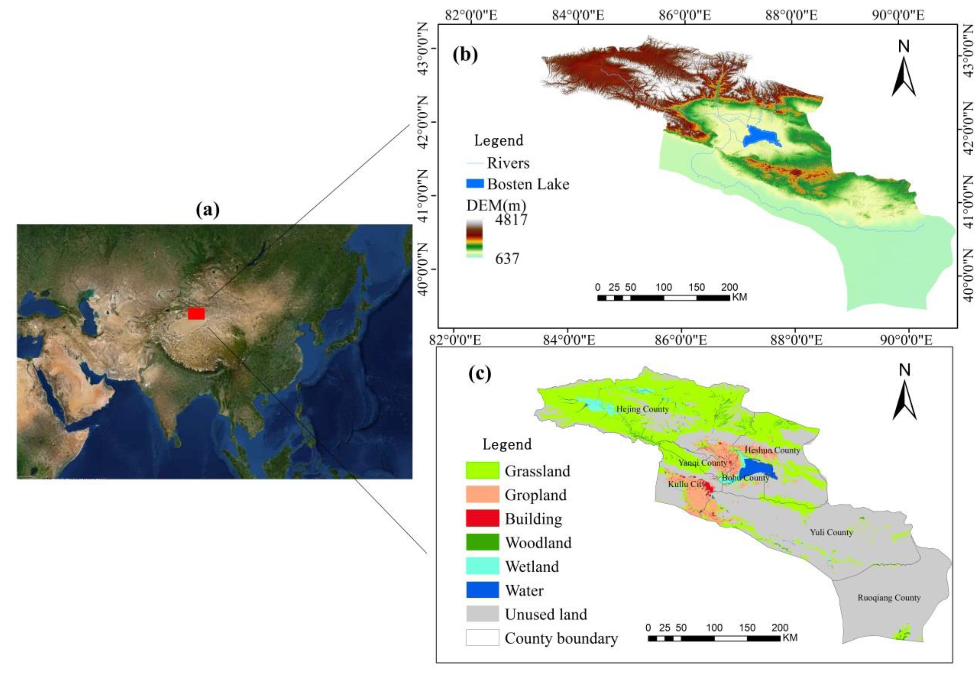
Figure 2.
The framework linking ecosystem service supply and social demand [27].
Figure 2.
The framework linking ecosystem service supply and social demand [27].

Figure 3.
Spatial distribution of ES supplies in the Kaidu-Kongque River Basin from 1990 to 2020.
Figure 4.
Spatial distribution of ES demands in the Kaidu-Kongque River Basin from 1990 to 2020.

Figure 5.
Spatial distribution of ESDRs in the Kaidu-Kongque River Basin from 1990 to 2020.

Figure 6.
Structure of ES supply (a) and demand (b) from 1990 to 2020 in the study area.

Figure 7.
ES mismatches from 1990 to 2020 in the study area.
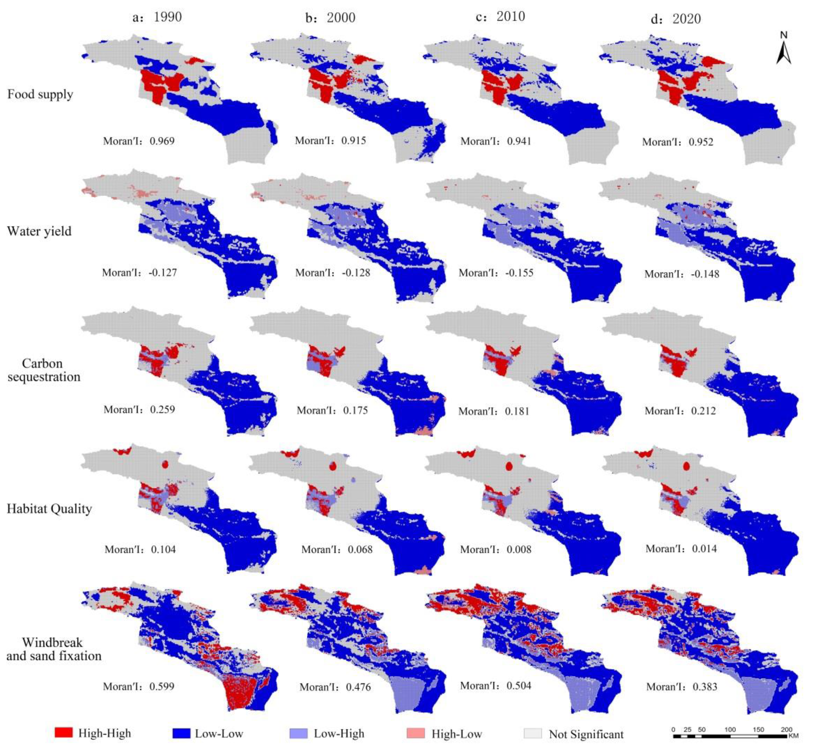
Table 1.
Data source and usage.
| Data Category | Usage | Source |
|---|---|---|
| Land use and land cover (LULC) data (1990~2020) | water yield; habitat quality; carbon sequestration; windbreak and sand fixation | http://www.resdc.cn, accessed on 1 December 2020. |
| Digital elevation model (DEM) | water yield | http://www.gscloud.cn/, accessed on 10 February 2021. |
| Normalized difference vegetation index (NDVI) (1990~2020) | food supply; windbreak and sand fixation | https://lpdaac.usgs.gov/, accessed on 4 January 2021. |
| Soil depth and texture data (1990~2020) | water yield; carbon sequestration; habitat quality; windbreak and sand fixation; | http://www.geodata.cn, accessed on 20 January 2021. |
| Biohabitat location data (1990~2020) | habitat quality | https://www.gbif.org/zh/dataset/, accessed on 1 February 2021. |
| Meteorological data (monthly precipitation, monthly evaporation, monthly temperature, monthly wind speed, and monthly solar radiation) (1990~2020) | water yield; windbreak and sand fixation | http://data.cma.cn, accessed on 11 March 2021. |
| Population density and gross domestic product (GDP) density data (1990~2020) | food demand; water demand; habitat quality demand; carbon sequestration demand | https://www.worldpop.org, accessed on 15 December 2020. https://www.gbif.org/zh/dataset/, accessed on 1 May 2021. |
| Grain yield and consumption data (1990~2020) | food demand; water demand | http://slt.xinjiang.gov.cn, accessed on 4 July 2021. |
| Nighttime light data (1990~2020) | carbon sequestration demand | https://www.ngdc.noaa.gov/eog/viirs, accessed on 1 May 2021. |
| Carbon density data (1990~2020) | carbon sequestration | http://www.cnern.org.cn/, accessed on 19 May 2021. |
Table 3.
ESDRs of five ESs counted by administrative divisions and the whole basin.
| Year | Ecosystem Service | ESDRs Counted by Administrative Divisions and the Whole Basin | ||||||
|---|---|---|---|---|---|---|---|---|
| Yuli County | Korla City | Heshuo County | Bohu County | Yanqi County | Hejing County | The Whole Basin | ||
| 1990 | food supply | 0.46 | 0.07 | 0.43 | 0.41 | 0.31 | 0.16 | 0.23 |
| water yield | −0.87 | −0.82 | −0.18 | −0.99 | −0.82 | 0.79 | 0.10 | |
| carbon sequestration | 1.00 | 0.95 | 0.99 | 1.00 | 0.99 | 1.00 | 0.99 | |
| habitat quality | 0.99 | 0.76 | 0.97 | 0.94 | 0.80 | 0.96 | 0.90 | |
| windbreak and sand fixation | −0.82 | −0.74 | −0.66 | −0.76 | −0.56 | −0.34 | −0.56 | |
| 2000 | food supply | 0.36 | 0.18 | 0.50 | 0.37 | 0.28 | 0.33 | 0.23 |
| water yield | −0.88 | −0.77 | −0.22 | −0.99 | −0.65 | 0.87 | 0.10 | |
| carbon sequestration | 0.99 | 0.88 | 0.98 | 0.97 | 0.92 | 1.00 | 0.99 | |
| habitat quality | 1.00 | 0.76 | 0.99 | 0.98 | 0.94 | 0.97 | 0.90 | |
| windbreak and sand fixation | −0.89 | −0.82 | −0.71 | −0.79 | −0.67 | −0.43 | −0.56 | |
| 2010 | food supply | 0.37 | 0.45 | 0.51 | 0.53 | 0.50 | 0.41 | 0.46 |
| water yield | −0.95 | −0.90 | −0.38 | −0.99 | −0.78 | 0.78 | 0.06 | |
| carbon sequestration | 0.97 | 0.71 | 0.97 | 0.91 | 0.86 | 0.98 | 0.94 | |
| habitat quality | 1.00 | 0.81 | 0.99 | 0.99 | 0.97 | 0.99 | 0.96 | |
| windbreak and sand fixation | −0.89 | −0.79 | −0.70 | −0.77 | −0.96 | −0.48 | −0.68 | |
| 2020 | food supply | 0.70 | 0.75 | 0.89 | 0.83 | 0.80 | 0.78 | 0.50 |
| water yield | −0.95 | −0.92 | −0.32 | −0.99 | −0.77 | 0.78 | 0.00 | |
| carbon sequestration | 0.96 | 0.63 | 0.94 | 0.84 | 0.84 | 0.97 | 0.92 | |
| habitat quality | 1.00 | 0.80 | 0.99 | 0.99 | 0.96 | 0.99 | 0.96 | |
| windbreak and sand fixation | −0.87 | −0.81 | −0.72 | −0.81 | −0.65 | −0.48 | −0.66 | |
Disclaimer/Publisher’s Note: The statements, opinions and data contained in all publications are solely those of the individual author(s) and contributor(s) and not of MDPI and/or the editor(s). MDPI and/or the editor(s) disclaim responsibility for any injury to people or property resulting from any ideas, methods, instructions or products referred to in the content. |
© 2023 by the authors. Licensee MDPI, Basel, Switzerland. This article is an open access article distributed under the terms and conditions of the Creative Commons Attribution (CC BY) license (https://creativecommons.org/licenses/by/4.0/).
Share and Cite
MDPI and ACS Style
Yan, Y.; Li, J.; Li, J.; Jiang, T. Spatiotemporal Changes in the Supply and Demand of Ecosystem Services in the Kaidu-Kongque River Basin, China. Sustainability 2023, 15, 8949. https://doi.org/10.3390/su15118949
AMA Style
Yan Y, Li J, Li J, Jiang T. Spatiotemporal Changes in the Supply and Demand of Ecosystem Services in the Kaidu-Kongque River Basin, China. Sustainability. 2023; 15(11):8949. https://doi.org/10.3390/su15118949
Chicago/Turabian StyleYan, Yujiang, Jiangui Li, Junli Li, and Teng Jiang. 2023. "Spatiotemporal Changes in the Supply and Demand of Ecosystem Services in the Kaidu-Kongque River Basin, China" Sustainability 15, no. 11: 8949. https://doi.org/10.3390/su15118949
Note that from the first issue of 2016, this journal uses article numbers instead of page numbers. See further details here.