Evaluation of Selected Algorithms for Air Pollution Source Localisation Using Drones

Abstract

Polluted air causes enormous damage to human health. There is a high demand to find a solution for locating the places of illegal waste incineration due to the persistent smog problem. The use of multi-rotor drones for that purpose has now become one of the important research topics. The aim of the work was to check the possibility of using simple algorithms to search for the source of pollution. The algorithms that require low computing power, which may be part of the robot’s measurement and the control system’s internal software, were considered. The focus was on building a system based on a single robot that independently searches an area of a certain size. The simulation of the accuracy and scalability of the three different search algorithms was analysed for areas up to 200 m × 200 m. Two multi-rotor robots were prepared for the fieldwork. The validation of the two selected algorithms was carried out in outdoor environmental conditions. The fieldwork tests were carried out in areas with a maximum size of 100 m × 100 m. The obtained results were different, in particular on the wind speed and direction and the intensity of the pollution source. The random influence of these factors can verify the operation of the proposed system in practical applications. The difference between the true and the position of the source indicated by the robot was up to 15 m. That difference depended on the mutual arrangement of the measurement points and the pollution source location.

1. Introduction

Industrial civilisation and the development of cities have brought humanity not only enormous prosperity, but also critical environmental problems. Constant air pollution has become the hallmark of our time and an integral part of the lives of city dwellers around the world. Polluted air, which causes enormous damage to human health, on the example of Poland alone, is responsible for the premature death of tens of thousands of people annually, the prevalence of allergies, and other types of diseases [1]. There are also less obvious costs, such as enormous expenses for healthcare or environmental costs, for, e.g., decaying building facades. Due to the persistent problem, there is a high demand to look for a solution that will enable the location of places of illegal waste incineration (pollution sources). The use of mobile robots (such as multi-rotor drones) to automatically search for a contamination source has now become one of the significant research topics. Robots of this kind, compared to traditional ones (the aircraft UAVs), are more flexible and safer.

Currently, research is being carried out on various types of dedicated flying robots. In the work [2], a dual-arm manipulator mounted on a multi-rotor platform was presented. The proposed design was evaluated through outdoor flight tests. Great possibilities in the field of robot positioning in the air can be provided by the solution presented in [3]. In that article, a fully actuated multi-rotor vehicle that can hover at any attitude and accelerate in any direction was described. As far as suitability for airborne measurement purposes is concerned, a [4] solution may be useful, where a single-rotor system was presented. In this case, the generated flow field disturbances would be the smallest; however, such a robot has the disadvantage of the lack of maintaining the yaw direction. As the authors pointed out, the presented robot was controllable in position only after removing its yaw state.

The available literature includes many published examples of the use of robots for widely understood environmental protection purposes. In particular, the work [5] presented a quadrotor design for outdoor air quality monitoring, made of easily obtainable and commercially available components. The influence of rotors on the measurement reliability was taken into account for three different cases of mounting the measurement system. However, this article did not present the actual unit for measuring air pollutants. A multi-rotor-based system for measuring gaseous pollutants was presented in [6]. It was equipped with the following semiconductor sensors: methane ${\mathrm{CH}}_4$, carbon monoxide CO, and carbon dioxide ${\mathrm{CO}}_2$, a sensor that reacts to several types of gases such as ${\mathrm{NH}}_3$, NOx, alcohol, and benzene, and a temperature sensor. The popular Arduino platform was used to collect the data. An interesting and innovative solution was presented in [7]. The presented robot used similar sensors as mentioned earlier, but the novelty lied in the fact that the robot can abate the detected air pollution. However, at this stage, the robot was equipped with the on-board pollution abatement for ${\mathrm{NO}}_2$ only. In addition, the effectiveness of such a solution was limited by the loading capacity of the robot. In [8], a small robot searched for a gas source (ethanol vapours) in a room. The robot moved at a constant height of 1.2 m in an area of 7 m × 12 m. However, in these examples, the robot was moving in a closed environment.

There are also flying robots equipped with particulate matter (PM) sensors. In work [9], the authors described multi-rotor robots for a vertical PM profile measurement, i.e., PM2.5 particles and ozone at heights up to 140 m. The article [10] was focused on the analysis and determination of the vertical profile of the distribution of particulate matter. The six-rotor robot was equipped with a PM2.5 sensor, and measurements were made at heights up to 1000 m. In [11], a low-cost sensor-based system was proposed, mounted on a quadrocopter robot. The proposed solution was verified on the campus of Mascara University in Algeria. The article [12] presented measurements carried out in the city during periods of heavy traffic with the use of a quadrocopter robot. A simple recorder based on the Arduino platform equipped with temperature, humidity, and particulate matter sensors was installed under the robot. A similar simple system was presented in [13]. Three-dimensional graphs of the measured values for exemplary flights were presented.

The air unsteady turbulent structures around a multi-rotor robot that directly interact with ambient particulate matter and gases are a challenging measurement issue. A preliminary analysis of the sensor placement location for a four-rotor robot was presented in [14]. The work [15] laid the groundwork for in-depth studies on how to measure particulate matter using multi-rotor robots. The authors conducted the experiments both in a wind tunnel and open-air, using a quadrotor-type robot. The obtained results showed the PM2.5 concentration increasing as much as 400% when comparing measurements taken before and after the propellers were turned on. Based on the research conducted in [16], it was decided to place the measurement system inlet on the raised platform about 50 cm above the robot. An analysis of the optimal measurement time was also presented.

When it comes to the pollution source searching algorithms, it should be noted, as the article [17] indicated, that the literature is mostly dominated by four types of methods of searching for pollution sources (robot active olfaction (RAO)). These are biological methods (imitating animals), methods involving fluid dynamics, statistical methods, and methods that use multiple robots. Each of the methods mentioned has its advantages and disadvantages.

A biological searching method with a single robot was presented in [18]. The algorithm of the pollution source searching was divided into several phases: active/passive search for a stream, stream tracing, and source identification. During the jet tracking phase, the robot moved upwind towards the source of pollution. The focus was on three tracking algorithms, with the most important the proprietary pseudo-gradient method, where the robot moved towards the source based on the gradient change. The measurement of wind and pollution concentration was performed in two places each time, and on this basis, a new direction of movement was determined. This approach is very simple to implement; however, the results may not be very repeatable. This approach involves moving towards the source upwind. A similar approach was presented in [19], where a robot and control algorithms for searching for the ${\mathrm{CO}}_2$ gas source in the tunnel were prepared. As the authors pointed out, it is necessary to further investigate the practicality of the proposed solution. A wide overview of the application of biological methods for the purposes of robot control and trajectory planning, as well as the directions of future research in this field was described in the work [20].

One of the well-known contamination source search algorithms today is the Infotaxis algorithm [21]. It is a source search algorithm without using gradient information. The search area, and thus the probability map, is gridded. Initially, equal probabilities of the presence of the pollution source at each location on the map are assumed. The search agent updates the probability map with each step. As the next position, the agent chooses the one that will result in the maximum information entropy drop. Research on this approach is still ongoing, such as the work [22]. The work mainly involved the study of different kinds of reward functions—Infotaxis, Infotaxis II, and Sinfotaxis variants—and the varying number of allowable directions the agent may travel for each step. An analysis was carried out for the 2D and 3D turbulent environments. However, these works did not take into account the influence of the rotors on the results obtained, and also, no practical tests in field conditions were carried out. Moreover, there was an impractical algorithm stop condition in the paper, which was that when the linear distance between the agent’s current position and the true location of the pollution source decreased below a certain threshold, the algorithm’s operation was stopped. Thus, it was assumed that the actual location of the pollution source being searched for was known.

There are also interesting systems utilising multiple robots [23]. In multiple robots systems, the coordination of many robots in space becomes a problem. Therefore, all robots must know their location and those of others. It is also mandatory to choose the number of robots appropriately for a given area because too many robots in too small an area will cause the robots to accidentally bump into each other continuously on a regular basis. It should also be noted that this method indirectly takes into account the possible presence of more than one source of contamination. Robots are looking for a global maximum. Other works that used multiple flying robots include [24], where simulation tests were presented, where in terms of time and performance, various methods of scanning a given space were compared, such as lawnmower, zigzag, spiral, and spindle. The work [25] presented a solution for the optimal division of the studied area between many flying robots and the planning of the robot’s route in a separate sub-area. However, that work did not include the practical implementation of the presented solution. The proposed algorithm also requires a priori information about the distribution of pollution in a given environment. Measurements were carried out at a constant height.

As other methods of searching for pollution sources (which are generally computationally complex), Reference [26] can be considered. There, two measurement algorithms were presented: for point sources (where the source location is known) and for an unknown location. The weakness of this work was that the measurements were made with the robot being manually controlled, and the data analysis was performed on the ground after all measurements had been taken. Based on these data, it was possible to determine the location of the carbon monoxide source in a case where its location was unknown and to estimate the intensity for a source with a known location in which the measurement was not performed directly. This category of computationally complex approaches also includes the neural-network-based approach, as in [27,28].

Summing up the research carried out over the last few years, some essential insights should be pointed out. The use of a multi-rotor drone to automatically search for a contamination source has now become one of the significant research topics. However, there is a lack of the practical implementation of simple and low-energy-demand search algorithms. The influence of rotors on measurement reliability should not be neglected especially for multiple robot systems. Some mentioned algorithms are sensitive to wind direction, and others assumed knowledge of true pollution source localisation.

The above-mentioned facts served as the primary motivation for this study where the objective was to develop a new single-robot system and algorithm for pollution source localisation. Another objective was the simulation and field comparison of the selected algorithms in the context of source localisation and energy demand.

The advantage of this work is that the research was performed in practical (variable) environmental conditions. Moreover, the implemented algorithms (and thus measurements and calculations) were performed during the flight. After taking off, the robot moved fully autonomously, searching for the pollution source. The points on which robot moved were not constant and were determined during the flight, based on the parameters set for the implemented algorithms. The proposed solution was characterised by low requirements for the computing power, and thus, subsequent measuring points can be quickly determined directly on the robot. The measurement data (particulate matter concentration) were sampled continuously and were available not only for the desired measurement points. Moreover, the measurement system was independent of the control system, and therefore, it was possible to test any algorithms and expand them in any desired way. The solution with one robot performing measurements in a designated area did not pose problems with the coordination of robots in the air.

2. Materials and Methods

In this section, the adopted research plan is presented. The first part presents the two flying robots constructed that were used to conduct the measurements. The following subsection describes the proposed and tested algorithms.

2.1. Constructed Drones

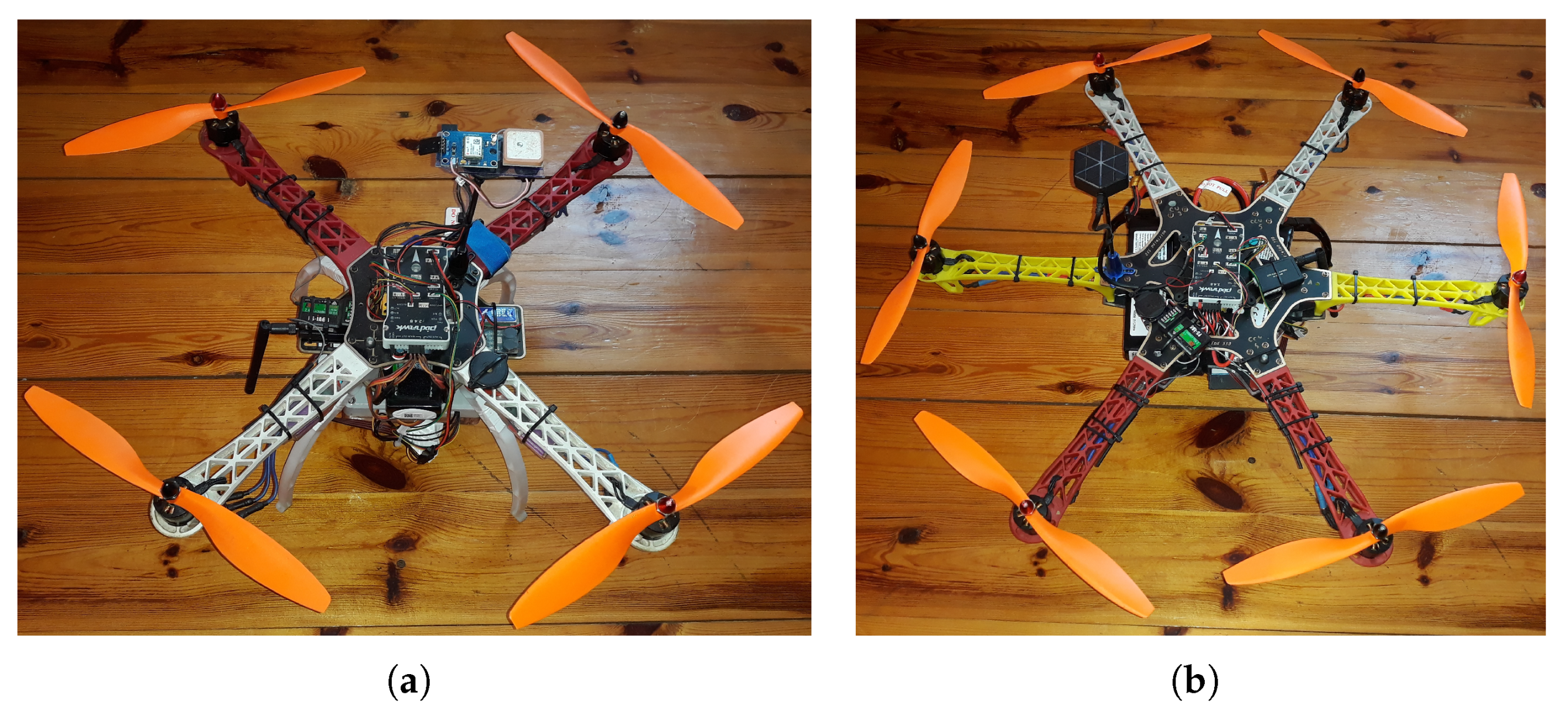
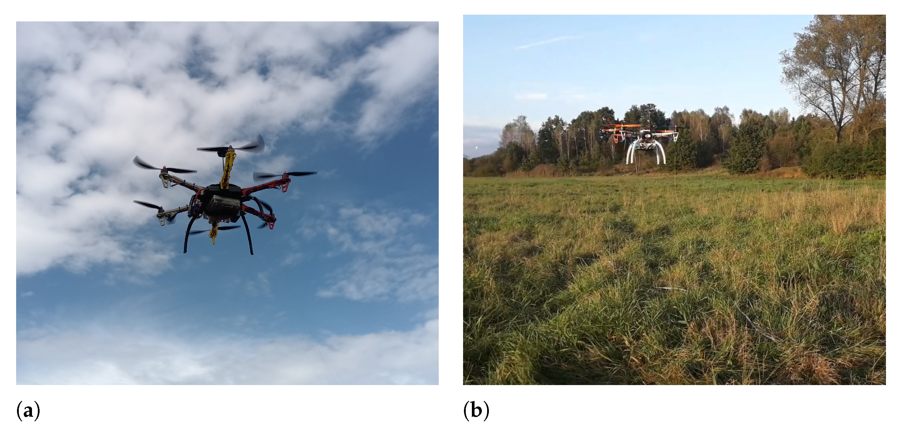
Two multi-rotor robots (as presented on Figure 1) were prepared for the fieldwork: a quadrocopter and a hexacopter. Due to the insufficient lifting capacity (and thus, short flight time) of the four-rotor robot, were needed to build a six-rotor robot. That robot was used primarily when the research was conducted in larger areas (100 m × 100 m). The quadrocopter robot was used during the research in a 60 m × 60 m area.

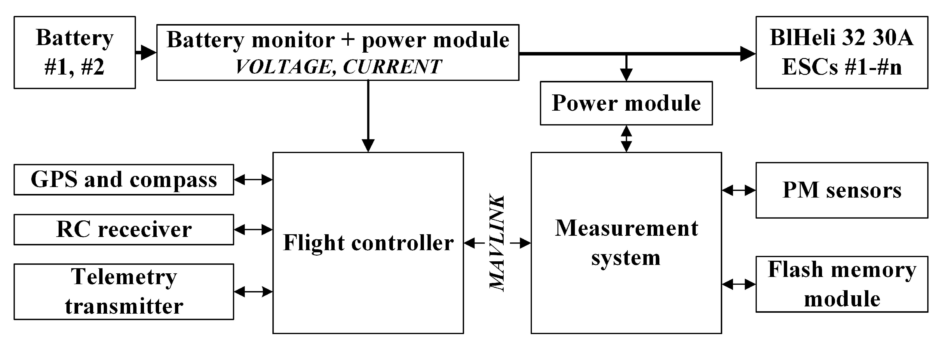
Both robots use EMAX MT2213 BLDC motors, a 30 A BlHeli-based ESC, and GEFMAN 10 × 4.5 (10 in long) propellers, four and six sets of these, respectively. A single drive set of this kind has a maximum of 860 g lifting capacity. That sums up to 3.44 kg for four rotors and 5.16 kg for six rotors. Each robot was built on the TAROT frames of Classes 450 and 550, respectively. This means that the largest distance between the motors was: 450 mm (four-rotor) and 550 mm (six-rotor). The general block diagram of the electrical system of the both robots is shown in Figure 2.

The smaller robot utilises a single 5000 mAh 3S (11.1 V nominal volt). LiPo battery. The bigger one can lift two 6500 mAh 3S LiPo’s (which is 13 Ah in total). The estimated times that each robot can hover in the air were 18.8 min and 29.9 min, respectively. The actual times during the field tests were about 15 min and 25 min, accordingly. The masses of the fully equipped robots were, respectively: 1.59 kg and 2.54 kg.

Last but not least, both robots were equipped with a Pixhawk flight controller and constructed measurement system, which is described in the next section. The flight controller was responsible for keeping the robot in the air. The measurement system took measurements and led the robot to the desired coordinates. Companion components, such as a GPS receiver, RC receiver, telemetry transmitter/receiver, and battery monitor, also belonged to the electronic equipment of each drone.

2.2. Description of the Constructed Measurement System

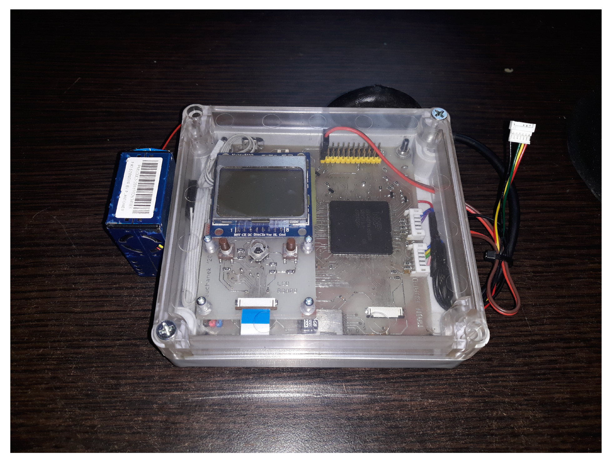
The constructed control measurement system was enclosed in a hard plastic housing with dimensions of 115 mm × 125 mm × 36 mm. It was powered by an independent 5V BEC power supply (which is a step-down power converter), completely separate from the flight controller supply.

Communication between the Pixhawk flight controller and constructed system was implemented in the hardware layer using the UART bus, while in the software layer, the Mavlink protocol was used. During the software preparation process, ready-made Mavlink protocol libraries [29] were used. The remaining parts of the software were prepared entirely independently.

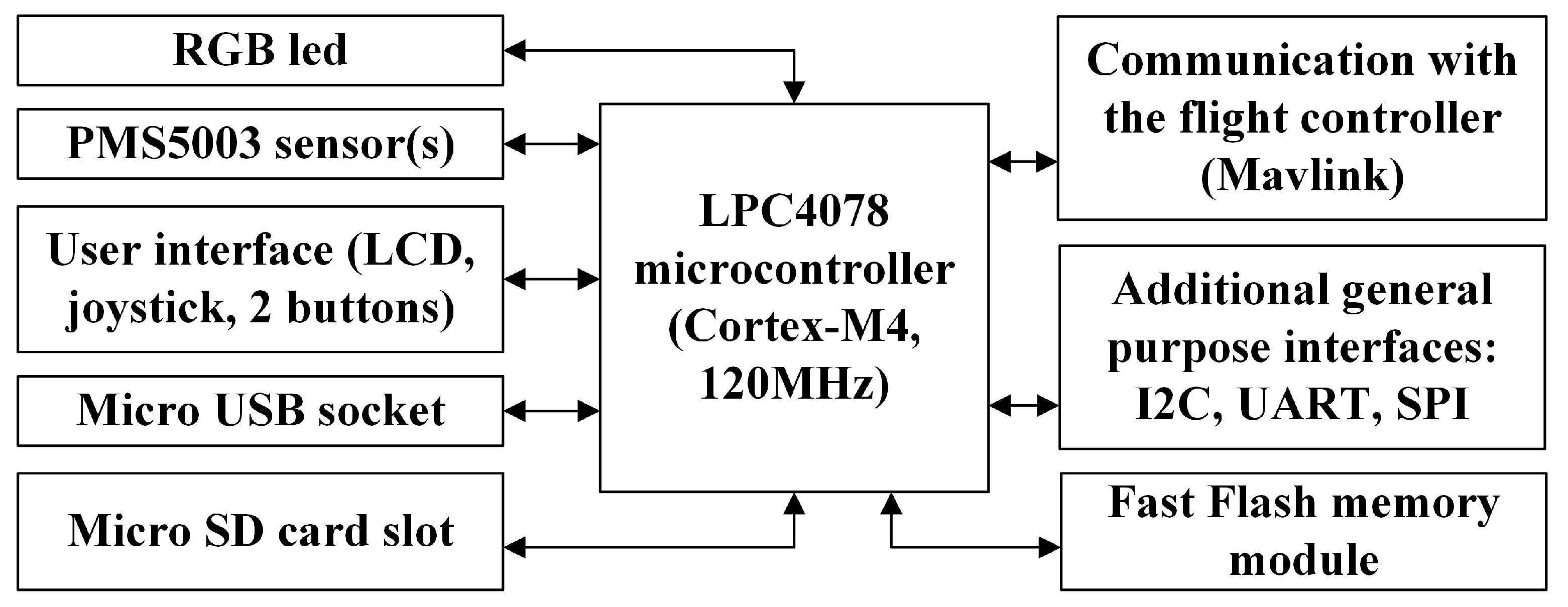
The most important components of the prepared system were an LPC4078 NXP Cortex-M4 120 MHz MCU, 256 Mb flash memory for data acquisition (approximately 35 min @ 500Hz), an RTC clock, and an LCD with a joystick and extra buttons, which comprise the user interface. A single Plantower PMS5003 [30] module was used as a particulate matter sensor. That sensor has the following (selected) measurement properties: range of measurement 0.3 ÷ 1.0 μm, 1.0 ÷ 2.5 μm, and 2.5 ÷ 10.0 μm, resolution of 1 μ/m³, single response of time < 1 s, and physical size of 50 mm × 38 mm × 21 mm. The total weight of the measurement system with one PM sensor was about 330 g. The general block diagram of the constructed control measurement system is shown in Figure 3.

The appropriate placement of the sensor in the disturbed air is important for the air to reach the sensor faster. A single sensor was centrally located with the control measurement system (Figure 4) under the drone for practical reasons. However, preliminary analyses were carried out in the Ansys software [14], where it was found where the area beyond the disturbances in the airflow field generated by the robot was located. It is planned to locate a second sensor on the extended arm, thanks to which it will be possible to compare both of their measurements.

2.3. Proposed and Tested Algorithms

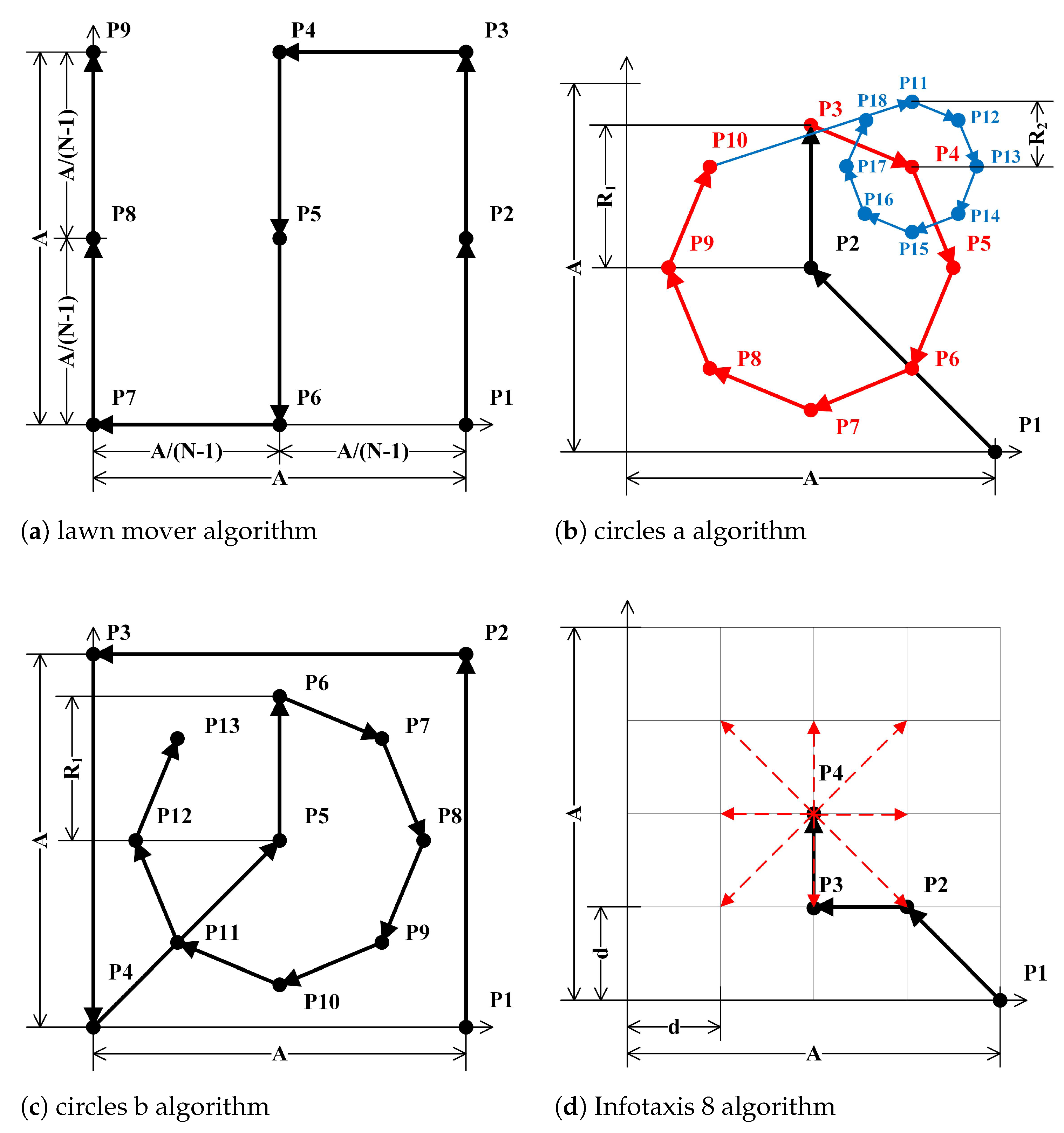
The first search algorithm—Figure 5a—mimics the operation of a lawnmower. In this case, the parameters of the algorithm are the side length of the square A and the number of measurement points along the side N. This approach has very low computing power requirements. In this case, as in every subsequent case, the robot starts the search from the (A, 0) coordinates. First, a grid of points is generated. Then, the robot performs successive measurements according to the sequence of points. After measurements are taken, the maximum value is found at all points and is considered the location of the source of contamination.

In the case of the second algorithm, two variants were analysed. In both cases, the robot starts searching from the lower right corner of the area (P1 point). In the case of the first variant (Figure 5b), the robot moves to the centre of the terrain (P2 point) and performs a flight in a circle with a radius of $R_1$ (red circle). Then, from these points, the point with the highest recorded concentration is selected (which was P4 in this example). Next, around this point, more points are generated on the circle with a (smaller) $R_2$ radius (blue circle). This procedure is repeated for a fixed number of steps, for more circles with decreasing diameters. In the case of the second variant (Figure 5c), the robot can make a preliminary flight around the terrain boundaries, i.e., (via P1, P2, P3, and P4 and then go to P5-centre), and then continue as for the first variant. The idea behind these extra points was related to the fact that if the source of contamination is outside the first circle and it dissipates outside of it, it may go undetected. In this case, the parameters of the algorithm were, as before, the side length of the A square, the number of points on the N circle (8), and the consecutive radii $R_1,R_2,\dots$ of the consecutive circles.

Low requirements characterise these algorithms regarding the computing power, and thus, subsequent measuring points can be quickly determined directly on the robot.

Another tested algorithm was Infotaxis [21]. This is a well-known contamination source search algorithm without using gradient information. The direct operation of the algorithm will not be discussed here; only the implementation details will be presented, as this algorithm was used to perform a comparison with simple solutions. The implementation in the Python [31] language available, and in particular the article [22], was used to implement Infotaxis in the MATLAB environment. Then, the operation of the following variants for the 2D space was tested: Infotaxis 4, Infotaxis 8, Infotaxis II 4, and Infotaxis II 8. Variants 4 and 8 differ from each other in terms of movement, where the next step can be performed in 4 or 8 directions, respectively. Infotaxis and Infotaxis II differ in their reward function, which is a criterion used to determine how the search agent moves. The scheme of operation of the Infotaxis algorithm is presented in the (Figure 5d). In this case, the area was divided into a grid of size d × d. The robot, starting from position (A, 0), moves along this grid, and from each position, it can move to 8 adjacent positions. In other words, it can move forward/backward, left/right, and diagonally, as shown in the picture. In the case when the robot is on the border of the search area, the number of possible positions is limited. This is necessary so that robot does not leave the designated area. For example, from the starting position (P1), the robot can only move to 3 adjacent positions.

A more detailed description of the operation of all algorithms is presented in the section on the simulation results.

3. Simulations Results

In order to initially assess the accuracy and the possibility of practical implementation, Algorithm 1 (lawnmower), Algorithm 2 (circles in Variants a and b), and Algorithm 3 (Infotaxis) were implemented and tested in the MATLAB software. Tests were performed for various cases of contamination field distribution. All algorithms were tested for the gas diffusion model given by the following equation [22] (Equation (1)):

$$C\left(r\right|r_s)=\frac{R}{2\pi D}{e}^{-(x-x_s)V/2D}{K}_0\frac{|r-r_s|}{\lambda },\lambda =\sqrt{\frac{D\tau }{1+V^2\tau /4D}}$$

(1)

where: V—average wind speed, D—effective isotropic diffusion coefficient, R—release rate of the release source, $\tau$—average life of particles released by the releasing source, $K_0$—Bessel function with a zero-order modification, $|r-r_s|$—linear distance between the current position of the search agent and the release source, and $C\left(r\right|r_s)$—particle concentration at r if the release source is at $r_s$.

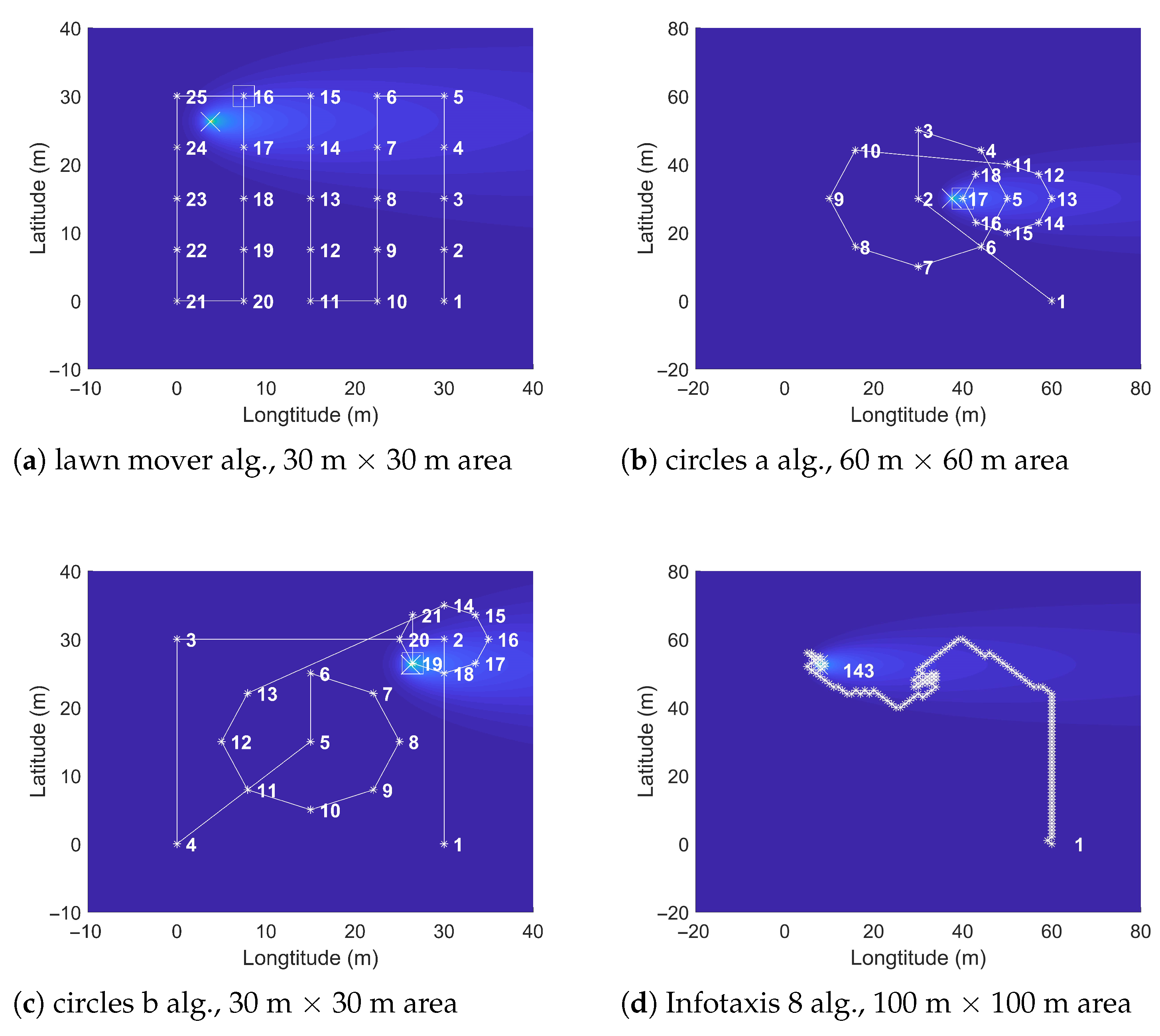
This model was used because it is the model on which the Infotaxis algorithm is based. The following model parameters were chosen: R = 100 Hz, V = 0.5 m/s, D = 0.6 m²/s, and τ = 500 s. For this model, the operation of all the given algorithms was analysed for areas with four different sizes: 30 m × 30 m, 60 m × 60 m, 100 m × 100 m, and 200 m × 200 m. The starting point was always a point with the coordinates (A, 0). For each case, the source of pollution was placed at the three different coordinates: ($\frac{7}{8}A$, $\frac{7}{8}A$)—i.e., in the top right corner, as in Figure 6c, ($\frac{1}{8}A$, $\frac{7}{8}A$)—in the top left corner, as in Figure 6a,d, and ($\frac{5}{8}A$, $\frac{1}{2}A$)—near the centre of the area, as in Figure 6b. This true location of the contamination source was not known by the search agent during the execution of any of the algorithms. For all 12 combinations (details are given in the Appendix A, in

Table A1. Algorithm 1 (lawn mover) operation for different cases: simulation data.

Location of Source	Str. Line Dist.	Total Trav. Dist.	Total Exec. Time	Time Meas. %	Dist. to Source	Comp. Time	Max Conc.	Min Conc.	Mean Conc.
30 m × 30 m area, start at (30 m, 0 m)
(3.75 m, 26.25 m)	37.12 m	180 m	255 s	29%	5.30 m	0.009 s	10.97	0.00	3.51
(18.75 m, 15.00 m)	18.75 m	180 m	255 s	29%	3.75 m	0.009 s	24.56	0.00	2.24
(26.25 m, 26.25 m)	26.52 m	180 m	255 s	29%	5.30 m	0.009 s	10.97	0.00	0.93
60 m × 60 m area, start at (60 m, 0 m)
(7.5 m, 52.5 m)	74.25 m	360 m	435 s	17%	23.72 m	0.009 s	5.72	0.00	1.62
(37.5 m, 30.0 m)	37.50 m	360 m	435 s	17%	7.50 m	0.009 s	17.57	0.00	1.22
(52.5 m, 52.5 m)	53.03 m	360 m	435 s	17%	10.61 m	0.009 s	4.06	0.00	0.32
100 m × 100 m area, start at (100 m, 0 m)
(12.5 m, 87.5 m)	123.74 m	600 m	675 s	11%	39.53 m	0.009 s	2.98	0.00	0.80
(62.5 m, 50.0 m)	62.50 m	600 m	675 s	11%	12.50 m	0.009 s	13.51	0.00	0.85
(87.5 m, 87.5 m)	88.93 m	600 m	675 s	11%	17.68 m	0.009 s	1.30	0.00	0.10
200 m × 200 m area, start at (200 m, 0 m)
(25 m, 175 m)	247.49 m	1200 m	1275 s	6%	127.48 m	0.009 s	0.97	0.00	0.22
(125 m, 100 m)	125.00 m	1200 m	1275 s	6%	25.00 m	0.009 s	9.18	0.00	0.54
(175 m, 175 m)	176.7 m	1200 m	1275 s	6%	-	0.009 s	0.10	0.00	0.01

,

Table A2. Algorithm 2a (circles) operation for different cases: simulation data.

Location of Source	Str. Line Dist.	Total Trav. Dist.	Total Exec. Time	Time Meas. %	Dist. to Source	Comp. Time	Max Conc.	Min Conc.	Mean Conc.
30 m × 30 m area, start at (30 m, 0 m)
(3.75 m, 26.25 m)	37.12 m	137 m	215 s	36%	4.51 m	0.015 s	22.27	0.02	10.06
(18.75 m, 15.00 m)	18.75 m	144 m	222 s	35%	1.25 m	0.015 s	39.75	0.00	10.57
(26.25 m, 26.25 m)	26.52 m	85 m	115 s	26%	-	0.015 s	0.29	0.00	0.04
60 m × 60 m area, start at (60 m, 0 m)
(7.5 m, 52.5 m)	74.25 m	275 m	353 s	22%	9.02 m	0.015 s	15.63	0.00	5.87
(37.5 m, 30.0 m)	37.50 m	288 m	366 s	21%	2.50 m	0.015 s	29.54	0.00	5.46
(52.5 m, 52.5 m)	53.03 m	170 m	200 s	15%	-	0.015 s	0.00	0.00	0.00
100 m × 100 m area, start at (100 m, 0 m)
(12.5 m, 87.5 m)	123.74 m	458 m	536 s	15%	15.04 m	0.015 s	11.75	0.00	3.70
(62.5 m, 50.0 m)	62.50 m	480 m	558 s	14%	4.17 m	0.015 s	23.38	0.00	3.25
(87.5 m, 87.5 m)	88.93 m	283 m	313 s	10%	-	0.015 s	0.00	0.00	0.00
200 m × 200 m area, start at (200 m, 0 m)
(25 m, 175 m)	247.49 m	916 m	994 s	8%	30.08 m	0.015 s	7.57	0.00	1.78
(125 m, 100 m)	125.00 m	960 m	1038 s	8%	8.33 m	0.015 s	16.67	0.00	1.70
(175 m, 175 m)	176.7 m	565 m	595 s	5%	-	0.015 s	0.00	0.00	0.00

,

Table A3. Algorithm 2b (circles modified) operation for different cases: simulation data.

Location of Source	Str. Line Dist.	Total Trav. Dist.	Total Exec. Time	Time Meas. %	Dist. to Source	Comp. Time	Max Conc.	Min Conc.	Mean Conc.
30 m × 30 m area, start at (30 m, 0 m)
(3.75 m, 26.25 m)	37.12 m	227 m	314 s	28%	4.51 m	0.02 s	22.27	0.00	9.31
(18.75 m, 15.00 m)	18.75 m	234 m	321 s	27%	1.25 m	0.02 s	39.75	0.00	9.49
(26.25 m, 26.25 m)	26.52 m	245 m	332 s	26%	0.30 m	0.02 s	66.29	0.00	8.56
60 m × 60 m area, start at (60 m, 0 m)
(7.5 m, 52.5 m)	74.25 m	455 m	542 s	16%	9.02 m	0.02 s	15.63	0.00	5.42
(37.5 m, 30.0 m)	37.50 m	468 m	555 s	16%	2.50 m	0.02 s	29.54	0.00	4.90
(52.5 m, 52.5 m)	53.03 m	490 m	571 s	15%	0.61 m	0.02 s	49.55	0.00	4.83
100 m × 100 m area, start at (100 m, 0 m)
(12.5 m, 87.5 m)	123.74 m	758 m	845 s	10%	15.04 m	0.02 s	11.75	0.00	3.41
(62.5 m, 50.0 m)	62.50 m	780 m	867 s	10%	4.17 m	0.02 s	23.38	0.00	2.92
(87.5 m, 87.5 m)	88.93 m	817 m	904 s	10%	1.01 m	0.02 s	38.62	0.00	3.18
200m × 200m area, start at (200 m, 0 m)
(25 m, 175 m)	247.49 m	1516 m	1603 s	5%	30.08 m	0.02 s	7.57	0.00	1.63
(125 m, 100 m)	125.00 m	1560 m	1647 s	5%	8.33 m	0.02 s	16.67	0.00	1.52
(175 m, 175 m)	176.7 m	1634 m	1721 s	5%	2.02 m	0.02 s	25.51	0.00	1.78

,

Table A4. Algorithm 3 (Infotaxis 8) operation for different cases: simulation data.

Location of Source	Str. Line Dist.	Total Trav. Dist.	Total Exec. Time	Time Meas. %	Dist. to Source	Comp. Time	Max Conc.	Min Conc.	Mean Conc.
30 m × 30 m area, start at (30 m, 0 m)
(3.75 m, 26.25 m)	37.12 m	109 m	374 s	71%	3.02 m	12.30 s	59.24	0.08	8.53
(18.75 m, 15.00 m)	18.75 m	81 m	275 s	70%	2.60 m	9.36 s	72.11	0.05	11.34
(26.25 m, 26.25 m)	26.52 m	78 m	274 s	72%	1.30 m	8.77 s	46.35	0.00	6.11
60 m × 60 m area, start at (60 m, 0 m)
(7.5 m, 52.5 m)	74.25 m	150 m	520 s	71%	1.61 m	63.30 s	46.15	0.00	6.78
(37.5 m, 30.0 m)	37.50 m	151 m	524 s	71%	1.50 m	65.61 s	56.65	0.01	6.51
(52.5 m, 52.5 m)	53.03 m	148 m	529 s	72%	2.65 m	60.22 s	46.15	0.00	5.48
100 m × 100 m area, start at (100 m, 0 m)
(12.5 m, 87.5 m)	123.74 m	236 m	851 s	72%	1.94 m	256.28 s	46.15	0.00	4.53
(62.5 m, 50.0 m)	62.50 m	160 m	555 s	71%	2.18 m	177.44 s	56.65	0.00	5.39
(87.5 m, 87.5 m)	88.93 m	140 m	526 s	73%	1.00 m	145.39 s	40.57	0.00	4.30
200 m × 200 m area, start at (200 m, 0 m)
(25 m, 175 m)	247.49 m	434 m	1548 s	72%	1.96 m	1795.85 s	113.52	0.00	2.69
(125 m, 100 m)	125.00 m	272 m	966 s	72%	0.94 m	1100.45 s	90.18	0.00	4.94
(175 m, 175 m)	176.7 m	258 m	976 s	74%	1.55 m	1023.17 s	113.52	0.00	3.15

), the following features were estimated: the total distance travelled by the robot, the total time of the robot’s operation, the percentage of this time used for the measurements, the distance between the true and the declared location of the pollution source, the time needed to calculate the algorithm, and the recorded concentrations—the highest, the lowest, and average. In the case of the Infotaxis algorithm, as the probability estimation was performed for the same model parameters as the input pollution model, the Poisson distribution was used to determine whether or not the robot had contact with the plume (hit or not). Therefore, the operation of this algorithm was not deterministic, and the values in the table were the mean values of three consecutive executions. It was also assumed here that the robot moved at a speed of 1 m/s, and the measurement of the concentration at one point took 3 s. The selected generated trajectories with measurement points marked for the algorithms that are discussed are presented in Figure 6. In Figure 6a, Algorithm 1 (lawnmower) for $A=30$ m and $N=5$ is presented. That means there were 25 measurement points, with a resolution (that is, the minimum distance between them) of 7.5 m. In Figure 6b, Algorithm 2 (circles) for $A=60$ m, $N=8$, $R_1=20$ m, and $R_2=10$ m and for $A=30$ m, $N=8$, $R_1=10$ m, and $R_2=5$ m (Figure 6c) is presented. The indicated parameters in these algorithms were entered manually and were constant during the operation. In the conducted research, the parameters were determined manually in such a way as to cover as much of the test area as possible, while avoiding the possibility of the robot moving outside the designated area. Primarily, in this case, this meant that the sum of the circles’ radii $R_1,R_2,\dots$ did not exceed half the width A of the designated area. The following dependencies were adopted during the tests, so $R_1=A/3$, $R_2=R_1/2$, and $R_{n+1}=R_n/2$. On the basis of the preliminary tests performed, the Infotaxis 8 algorithm showed the best performance, and therefore, this variant was used to perform a comparison with the simple algorithms presented earlier. An exemplary implementation is presented in Figure 6d. The square area (with side $A=60$ m) on which the search was carried out (and thus, the probability map) was divided into 1 m × 1 m sub-areas. The robot took measurements one by one and updated the probability map based on whether or not it had been in contact with the plume. It then took a step in one of eight directions which, resulted in maximum information entropy drop. The background for each of the presented case was the plume profile, where darker colours mean lower concentrations, warmer being higher. The exact location of the source of pollution, where the concentration was the highest, is marked with a white cross. This exact position was not known during the operation of one of the presented algorithms; the input parameter was only the contamination field distribution. At the current stage, it was also assumed that there would be only a single pollution source present in the searched area.

Each sub-figure of Figure 6 shows the order of the visited points. The route followed by the robot (which is the search agent) is marked with a white line. The robot starts searching the area from Point Number 1. The points where the measurements were made are marked with white asterisks. The robot successively takes measurements at designated points and, based on the concentrations measured there, decides how to move further. The final designated location that the robot considers to be the source of contamination is marked with a white square. In each case, it was assumed that the area in which the search for the source of pollution would be conducted had the shape of a square.

In

Table 1. Comparison of algorithms’ operation for an increasing area source in the top left corner: simulation data.

Alg.	Total Trav. Dist.	Total Exec. Time	Time Meas. %	Dist. to Source	Comp. Time	Max Conc.	Min Conc.	Mean Conc.
30 m × 30 m area , start at (30 m, 0 m), source at (3.75 m, 26.25 m), the straight-line distance to the source from the start point is 37.12 m
1	180 m	255 s	29%	5.3 m	0.009 s	10.97	0.00	3.51
2a	137 m	215 s	36%	4.51 m	0.015 s	22.27	0.02	10.06
2b	227 m	314 s	28%	4.51 m	0.020 s	22.27	0.00	9.31
3	109 m	374 s	71%	3.02 m	12.30 s	59.24	0.08	8.53
60m × 60 m area, start at (60 m, 0 m), source at (7.5 m, 52.5 m), the straight-line distance to the source from the start point is 74.25 m
1	360 m	435 s	17%	23.72 m	0.009 s	5.72	0.00	1.62
2a	275 m	353 s	22%	9.02 m	0.015 s	15.63	0.00	5.87
2b	455 m	542 s	16%	9.02 m	0.020 s	15.63	0.00	5.42
3	150 m	520 s	71%	1.61 m	63.30 s	46.15	0.00	6.78
100 m × 100 m area, start at (100 m, 0 m), source at (12.5 m, 87.5 m), the straight-line distance to the source from the start point is 123.74 m
1	600 m	675 s	11%	39.53 m	0.009 s	2.98	0.00	0.80
2a	458 m	536 s	15%	15.04 m	0.015 s	11.75	0.00	3.70
2b	758 m	845 s	10%	15.04 m	0.020 s	11.75	0.00	3.41
3	236 m	851 s	72%	1.94 m	256.28 s	46.15	0.00	4.53
200 m × 200 m area, start at (200 m, 0 m), source at (25 m, 175 m), the straight-line distance to the source from the start point is 247.49 m
1	1200 m	1275 s	6%	127.48 m	0.009 s	0.97	0.00	0.22
2a	916 m	994 s	8%	30.08 m	0.015 s	7.57	0.00	1.78
2b	1516 m	1603 s	5%	30.08 m	0.020 s	7.57	0.00	1.63
3	434 m	1548 s	72%	1.96 m	1795.85 s	113.52	0.00	2.69

, the operation of the algorithms for a growing terrain is shown. The pollution source was located in the ($\frac{1}{8}A$, $\frac{7}{8}A$) position. The designation of the algorithms in the table is as follows: 1—lawn mover, 2—circles (a/b variants), 3—Infotaxis 8. The detailed simulation results can be found in the Appendix A, in Table A1, Table A2, Table A3, Table A4.

In each case, it can be noticed that the distance travelled by the robot, and thus the algorithm execution time, increased, and this was due to the fact that there was an increasing area to be searched. The circles (a) algorithm was characterised by a shorter distance travelled; in the (b) version, the distance travelled was longer than in the lawn mower algorithm. The execution time of the Infotaxis algorithm was the longest, which was related to the large number of measurements performed, and thus their large percentage share in the total execution time. In the case of this algorithm, the assumed measurement time could be shortened by improving the result, because the travelled distances in each step were small in this case.

In the case of the simple algorithms, the accuracy of the localisation of the source of pollution deteriorated with the increasing size of the terrain. This was related to the parametric definition of the parameters of these, and thus, the distances between the generated points were greater. For the constant efficiency of the source for the increasing area, lower maximum values of the concentrations were also noted. However, it can be seen here that scalability was possible for these algorithms, however at the cost of accuracy. In the case of Infotaxis, the distance to the source was mostly unchanged, as the map resolution was kept invariably at 1m. However, when it came to the computational complexity, the Infotaxis algorithm has much higher requirements in terms of computing power, and thus, the computation time was much greater than the others. That time also grew rapidly due to the fact that it was necessary to perform operations on matrices (map) with increasing dimensions of: 31 × 31, 61 × 61, 101 × 101, and 201 × 201, respectively. Moreover, these cited examples, e.g., [22], were based on the impractical stop condition of the Infotaxis algorithm, whereby when the distance between the position of the search agent and the source of contamination decreases below a predetermined threshold, the robot is considered to have found the source of contamination. This is a condition that makes the practical implementation of the algorithm pointless, because since the location of the source is known a priori, there is no need to search for it. Instead, an condition involving the decrease in information entropy was used, which turned out to give satisfactory results. If at a given step, the calculated entropy value dropped below 10% of the original value, the algorithm stopped. The maximum value was then found on the probability map, which should be the same as (or close to) the true source of the pollution. This position was considered to be the declared final position of the pollution source.

In the event of a situation that the values measured at the concentration points did not exceed the threshold value (set at one), it was considered that the robot did not find the source of pollution. Then, in the corresponding row of the table, instead of the value of the distance to the pollution source, the sign “-” is inserted. In the case of the lawn mower algorithm, this was the case when this threshold value was not exceeded at all points. However, in the case of the circles algorithm, this was the case when the threshold value was not exceeded after the first circle flight. A failure of the case of the Infotaxis algorithm occurred when a predetermined condition (decrease in entropy) would not be reached after the maximum number of steps (set at 500) for the algorithm had been performed.

In

Table 2. Comparison of algorithms’ operation for a different pollution source location: 60 m × 60 m area; simulation data.

Alg.	Total Trav. Dist.	Total Exec. Time	Time Meas. %	Dist. to Source	Comp. Time	Max Conc.	Min Conc.	Mean Conc.
60 m × 60 m area, start at (60 m, 0 m), source at (37.5 m, 30.0 m), the straight-line distance to the source from the start point is 37.5 m
1	360 m	435 s	17%	7.50 m	0.009 s	17.57	0.00	1.22
2a	288 m	366 s	21%	2.50 m	0.015 s	29.54	0.00	5.46
2b	468 m	555 s	16%	2.50 m	0.020 s	29.54	0.00	4.90
3	151 m	524 s	71%	1.50 m	65.61 s	56.65	0.01	6.51
60 m × 60 m area, start at (60 m, 0 m), source at (52.5 m, 52.5 m), the straight-line distance to the source from the start point is 53.03 m
1	360 m	435 s	17%	10.61 m	0.009 s	4.06	0.00	0.32
2a	170 m	200 s	15%	-	0.007 s	0.00	0.00	0.00
2b	490 m	571 s	15%	0.61 m	0.020 s	49.55	0.00	4.83
3	148 m	529 s	72%	2.65 m	60.22 s	46.15	0.00	5.48
60 m × 60 m area, start at (60 m, 0 m), source at (7.5 m, 52.5 m), the straight-line distance to the source from the start point is 74.25 m
1	360 m	435 s	17%	23.72 m	0.009 s	5.72	0.00	1.62
2a	275 m	353 s	22%	9.02 m	0.015 s	15.63	0.00	5.87
2b	455 m	542 s	16%	9.02 m	0.020 s	15.63	0.00	5.42
3	150 m	520 s	71%	1.61 m	63.30 s	46.15	0.00	6.78

, the operation of the algorithms for a different pollution source location, on a 60 m × 60 m area, is presented.

Based on the results in Table 2, it can be noticed that for all algorithms, the total travelled distance and, thus, the execution time of the robot did not change significantly. The execution time of the Infotaxis algorithm was longer than that of the lawn mower algorithm. This was due to the fact that with Infotaxis, the most measurements were performed. However, in the case of the simple algorithms, the robot could move at a higher speed, which would also significantly reduce the execution time, as in these cases, the percentage of measurements was (roughly about three times) lower.

In the case of simple algorithms, the accuracy achieved varied. This was related to the mutual relationship between the generated points and the true location of the source of pollution. In the case of Infotaxis, the accuracy was much better. In the case when the pollution source was located at the location (52.5 m, 52.5 m), the circles (a) algorithm did not find the source of pollution, because in this case, the pollution was in a corner and spread outside the designated area. In this case, Variant b works well, but then, the robot will leave the designated area where the search was being carried out. This corresponds to the situation in Figure 5c. However, in this case, the distance travelled was even greater than in the lawn mower algorithm, and in addition, under different conditions, the performance was the same as in Variant a. Therefore, Variant b should be considered ineffective. However, for such conditions and in practical conditions, the operation of all the given algorithms may be unsatisfactory.

4. Measurement Results and Discussion

The aim of the work was to check the operation of simple algorithms in environmental conditions. Therefore, simple algorithms were used first for the practical implementation. The general operation of the lawn mover and circles is shown in Figure 7 and is as follows: for safety reasons, the robot was armed (which means the motors were enabled and the robot was ready to take off the ground) in manual mode (with auto-levelling). The operator took off and then put the robot in position hold mode. Then, automatic the operation could be enabled, and the robot:

• Generated the measuring points that needed to be checked;
• Took a measurement at the starting point (measurement is understood as the maximum recorded atmospheric concentration $P{M}_{10}$ during 3 s);
• The robot’s flight controller was switched to guided mode, thus disallowing the operator to override the robot’s position manually. The robot started an autonomous search of the area.

Figure 7. The general block diagram of the robot’s operation.

Figure 7. The general block diagram of the robot’s operation.

The robot then went to the generated points one by one and took measurements at them. After the first batch of points was checked, more were generated depending on the selected algorithm. After reviewing all points, the robot picked the point where the highest concentration was recorded and went to that point. After reaching its destination, the robot remained at this point in position hold mode. Each of the individual operating modes was indicated by the changing colour (as shown on Figure 7) of the multi-coloured LED with which the measuring system was equipped. The operator can abort the robot’s automatic operation at any time and take manual control over it. Other safety measures, such as emergency landing or return to home (RTH) modes, can also be triggered at any time.

In an area free of obstacles and away from buildings, traffic, or pedestrians, markers limiting the search area were placed. Next, the location of the pollution source was then selected at the site. The measurement of the emission source location was made with a tape measure relative to the starting point. The measurement system had no information about this true location; it was only used to determine the accuracy of the pollution source localisation algorithm. Then, the robot took off at the starting point, and after checking that the flight control system correctly responded to the pilot’s commands, it was switched to automatic search for pollution source. After that, the robot continued to execute the algorithm selected by the operator, as described in the previous section.

During the tests, the robot maintained a constant orientation and flew at a regular height of 4 m. The pollution source was located at the height of 0.5 m. The speed of the robot’s movement was set constant for both robots and was limited to a maximum of 0.75 m/s.

Figure 8 shows the constructed drones during the field tests: the quadrocopter during the take-off and the hexacopter in the air while navigating to the next point.

To verify the proposed algorithms, many measurements were made. In Figure 9, Figure 10, Figure 11, Figure 12 and Figure 13, several selected measurements are shown with the approximate location of the pollution source marked. The results of the operation for both implemented algorithms are presented. For each of the given cases, the following were calculated: the distance between the true location and the location of the pollution source indicated by the robot and the total algorithm execution time.

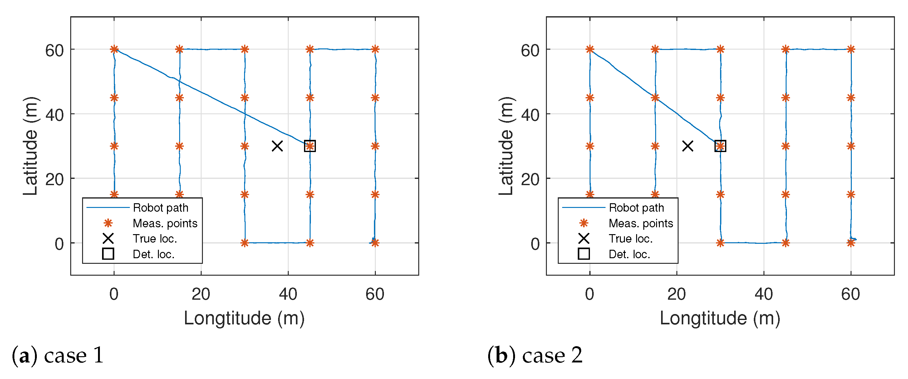
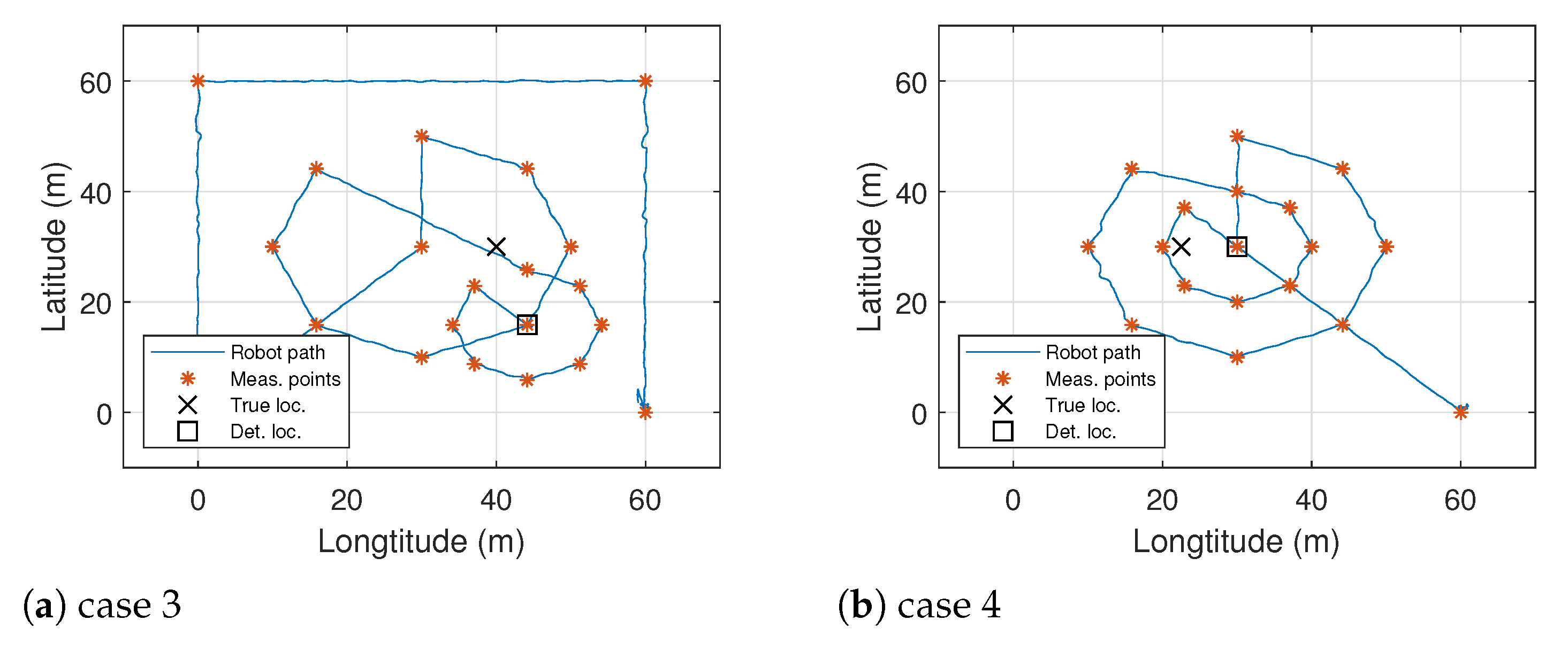
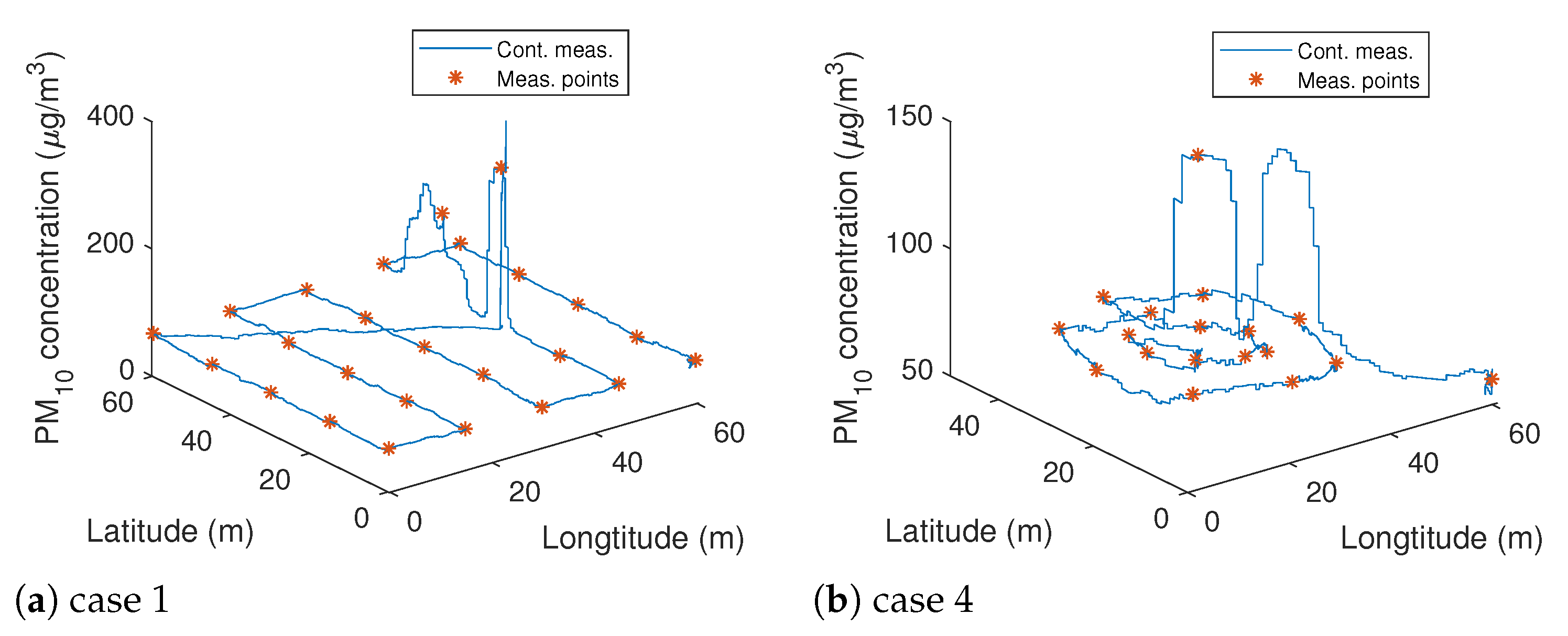
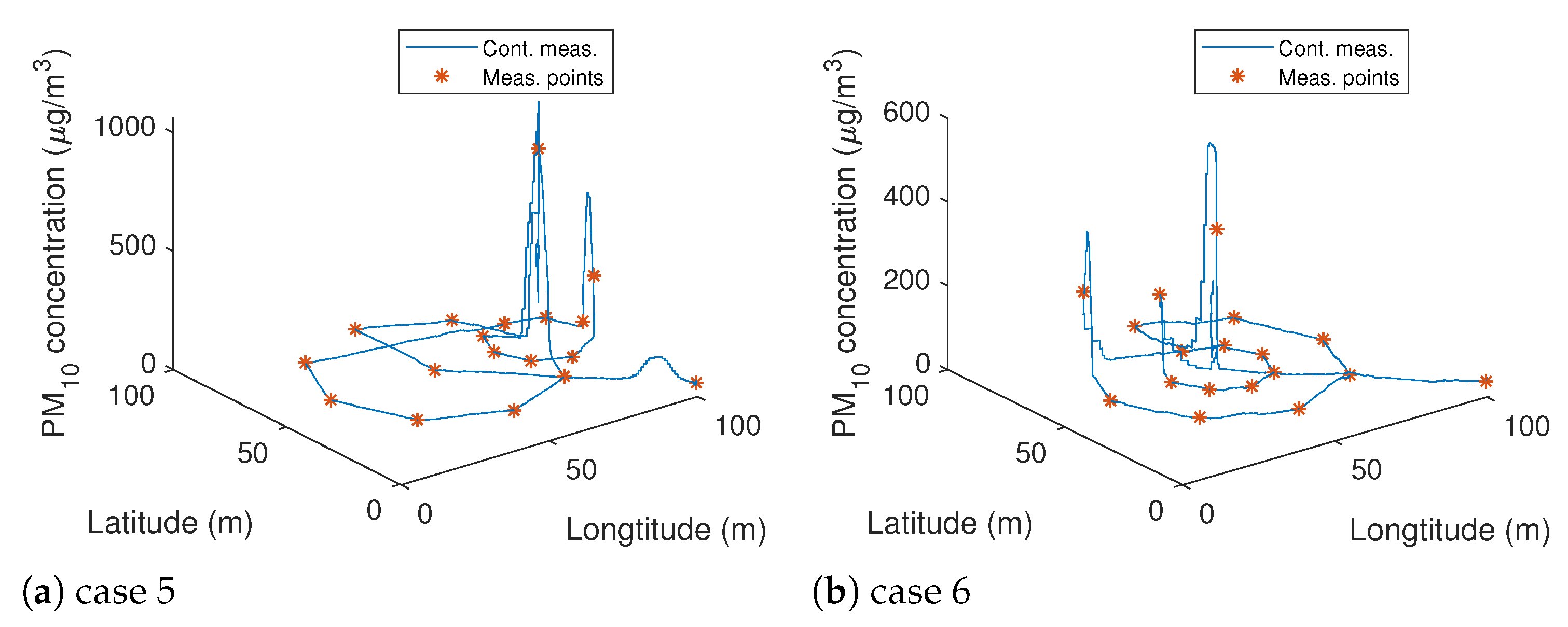
As can be observed, two types of charts are presented. Figure 9, Figure 10 and Figure 12 show: the travelled path by the robot (blue line), the measurement points (orange marks), the true pollution source location (big black cross), and the pollution source location determined by the robot (big black square) on the 2D plane. Figure 11 and Figure 13 show the continuous (blue line) and spot (orange marks) $P{M}_{10}$ measurements in 3D. The spot measurement is the maximum $P{M}_{10}$ concentration observed during 3 s at the current location.

During the tests, it could be observed that the obtained results were influenced in particular by: the wind speed and direction and the intensity of the pollution source. These parameters can be observed on the continuous measurement curves presented in the 3D graphs (Figure 11 and Figure 13). The random influence of these factors was to verify the operation of the proposed system in practical applications. The pollution source localisation’s effectiveness varied, but we can generally say that the robot was heading towards the proper source location.

Both algorithms were tested in a 60 m × 60 m area. Figure 9 shows examples of the operation for the first algorithm. The parameters were as follows: $A=60$ m, $N=5$. In both cases, the difference in the distance between the true location and the location of the pollution source indicated by the robot was equal to 7.5 m. The algorithm execution time was 10 min 39 s and 10 min 22 s, respectively.

Figure 10 shows the travelled paths for the second algorithms. Two variants are presented: when the robot makes a preliminary flight around the terrain boundaries or goes straight to the centre first. In both cases, the parameters were as follows: $A=60$ m, $N=8$, $R_1=20$ m, and $R_2=10$ m. The location of the source was determined with an error of 14.73 m and 7.5 m, respectively. The algorithm execution time was 11 min 14 s and 6 min 31 s, respectively. The shorter execution time was due to the preliminary flight’s omission around the test area boundaries. Moreover, when interpreting the results, one should also take into account the fact that the true location of the source was determined roughly with the help of a measuring tape. For two of the selected described cases above, the continuous measurements are presented in Figure 11. On the basis of these, it was possible to observe the propagation of pollution under the influence of wind.

Figure 12 shows examples of the operation for the second algorithm in a 100 m × 100 m area. The parameters were as follows: $A=100$ m, $N=8$, $R_1=35$ m, and $R_2=15$ m. In the fifth case (Figure 12a and Figure 13a), the location of the source was determined with an error of 5 m, within 11 min 7s. In the sixth case (Figure 12b), the source of pollution was placed in the centre of the site. In this case, the difference between the true pollution source localisation and that determined by the robot was equal to 0 m. Moreover, the contamination propagation can be observed in the course of the continuous measurement (Figure 13b). On the basis of this and previous measurements, a decrease in the measured $P{M}_{10}$ concentrations with the increasing distance from the source can be observed, which confirmed the compliance with the physical phenomenon of the dispersion of pollutants in the air. The algorithm execution time was 10 min 19 s in that case.

The scale of the pollution source must be adequate to the scale of the terrain. In all cases for the used source of increased concentration compared to the background, this can be seen only in the nearest measurement points (Figure 11 and Figure 13). If the source were not so intense, in that the concentration in one of the measurement points is significantly higher than in the others, it might not be detected.

The numerical values for all the discussed cases are presented in

Table 3. Summary of all presented cases: experimental data.

Case	Alg.	Area	No. of Points	Exec. Time	Dist. to Source	Max ${\mathit{PM}}_{10}$ Conc.	Min ${\mathit{PM}}_{10}$ conc.	Mean ${\mathit{PM}}_{10}$ Conc.
1	1	60 m × 60 m	25	10 m 39 s	7.5 m	314 μg/m3	58 μg/m3	80.6 μg/m3
2	1	60 m × 60 m	25	10 m 22 s	7.5 m	125 μg/m3	58 μg/m3	69.8 μg/m3
3	2	60 m × 60m	21	11 m 14 s	14.73 m	34 μg/m3	23 μg/m3	28.6 μg/m3
4	2	60 m × 60 m	18	6 m 31 s	7.5 m	138 μg/m3	60 μg/m3	68.3 μg/m3
5	2	100 m × 100 m	18	11 m 7 s	5.0 m	858 μg/m3	47 μg/m3	115.6 μg/m3
6	2	100 m × 100 m	18	10 m 19 s	0.0 m	367 μg/m3	31 μg/m3	72.8 μg/m3

. The table shows for each particular case number: the algorithm type (1 or 2) used, the area size, the number of measurement points, the algorithm execution time, the distance between the true and determined source location, and the maximum, minimum, and average values of the particulate matter $P{M}_{10}$ concentrations for all measurement points. From these values, it can also be concluded that when the ratio of the maximum measured concentration to the background concentration (that is, the mean value) was small, the performance of the algorithms was the worst (case 3). For the the example of the 60 m × 60 m area, the shortest search time was obtained for the proposed Algorithm 2 (Case 4). Compared to Algorithm 1 (Case 2), it was shorter by about 37.1%.

5. Conclusions

As indicated in the discussion of the results, the practical usefulness of the proposed solution can be stated. The robot carried out the measurements in accordance with the specified method. The most important conclusions from the presented work are as follows:

• The advantage of the proposed solution is the fact that the implemented algorithms (and thus, measurements and calculations) are performed on the go during the flight;
• The execution time of the algorithms (resulting directly from the path that the robot has to travel) in the case of the second algorithm was shorter by about 37.1% compared to the first. Of course, this time can be significantly reduced by increasing the speed of the robot’s flight;
• The scale of the pollution source must be adequate to the scale of the terrain. The source must be so intense that the concentration in one of the measurement points is significantly higher than in the others;
• The Infotaxis algorithm in the case of the simulation tests was characterised by the best accuracy; however, its practical implementation (related to the need to adopt source parameters that are unknown and due to the computational complexity) is troublesome;
• It is mandatory to add thresholding to find out if the source is present or not after the first phase of the flight. In the case of particulate matter, it seems that it may be dynamically determined, e.g., based on exceeding the average (e.g., $30\%$) after the first pass;
• The PM sensor measures so relatively quickly that it might be concluded that the robot does not have to stay at the point for quite a long time (3 s). When the robot approaches the source, a very violent disturbance occurs, which causes the contaminants to reach the sensor very quickly. This applies, of course, to a situation when the robot is moving relatively slowly, with speeds of 0.5 m/s and 0.75 m/s. The average response time of the sensor was 800 ms, which gives a measurement of 40 cm and 60 cm, respectively. At these speeds, it is possible, and desirable with more complex algorithms, to use data from the flight between measurement points;
• The proposed algorithm worked well for both robots used. The decision to choose a quadrocopter or hexacopter robot is dependent on the size of the search area.

It is important to take additional measurements with the second sensor mounted on the extended arm and to compare it with the sensor located at the centre under the robot. Data from both sensors can be registered simultaneously and also can be used simultaneously. Furthermore, it might be difficult to use drones in harsh weather conditions, especially in winter, when it is raining/snowing. However, at that time, and most often, the practice of burning low-quality fuel and garbage in home furnaces is present.

A more elaborate algorithm that can use available and unused current data should be implemented. In this case, this means the possibility of the use of data between measurement points. The particulate matter concentration is measured continuously. On this basis, it is possible to locate the source location more precisely.

References

- World Health Organization. Health Effects of Particulate Matter. Policy Implications for Countries in Eastern Europe, Caucasus and Central Asia. 2013. Available online: https://www.euro.who.int/en/health-topics/environment-and-health/air-quality/publications/2013/health-effects-of-particulate-matter.-policy-implications-for-countries-in-eastern-europe,-caucasus-and-central-asia-2013 (accessed on 20 February 2021).
- Suarez, A.; Jimenez-Cano, A.E.; Vega, V.M.; Heredia, G.; Rodriguez-Castaño, A.; Ollero, A. Design of a lightweight dual arm system for aerial manipulation. Mechatronics 2018, 50, 30–44. [Google Scholar] [CrossRef] [Green Version]
- Brescianini, D.; D’Andrea, R. An omni-directional multirotor vehicle. Mechatronics 2018, 55, 76–93. [Google Scholar] [CrossRef]
- Zhang, W.; Mueller, M.W.; D’Andrea, R. Design, modeling and control of a flying vehicle with a single moving part that can be positioned anywhere in space. Mechatronics 2019, 61, 117–130. [Google Scholar] [CrossRef]
- Koziar, Y.; Levchuk, V.; Koval, A. Quadrotor Design for Outdoor Air Quality Monitoring. In Proceedings of the 2019 IEEE 39th International Conference on Electronics and Nanotechnology (ELNANO), Kyiv, Ukraine, 16–18 April 2019; pp. 736–739. [Google Scholar] [CrossRef]
- Mazeh, H.; Saied, M.; Clovis, F. Development of a Multirotor-Based System for Air Quality Monitoring. In Proceedings of the Third International Conference on Electrical and Biomedical Engineering, Clean Energy and Green Computing (EBECEGC2018), Beirut, Lebanon, 25–27 April 2018; pp. 23–28. [Google Scholar] [CrossRef]
- Rohi, G.; Ejofodomi, O.; Ofualagba, G. Autonomous monitoring, analysis, and countering of air pollution using environmental drones. Heliyon 2020, 6, e03252. [Google Scholar] [CrossRef] [PubMed] [Green Version]
- Kurotsuchi, K.; Tai, M.; Takahashi, H. Vision-based autonomous micro-air-vehicle control for odor source localization. Adv. Sci. Technol. Eng. Syst. J. 2017, 2, 1152–1158. [Google Scholar] [CrossRef] [Green Version]
- Wang, Q. Real-time atmospheric monitoring of urban air pollution using unmanned aerial vehicles. WIT Trans. Ecol. Environ. 2019, 1, 79–88. [Google Scholar] [CrossRef] [Green Version]
- Wang, D.; Wang, Z.; Peng, Z. Using unmanned aerial vehicle to investigate the vertical distribution of fine particulate matter. Int. J. Environ. Sci. Technol. 2019, 17, 219–230. [Google Scholar] [CrossRef]
- Zareb, M.; Bakhti, B.; Bouzid, Y.; Kadourbenkada, H.; Bouzgou, K.; Nouibat, W. Novel Smart Air Quality Monitoring System Based on UAV Quadrotor. In Proceedings of the 4th International Conference on Electrical Engineering and Control Applications, Constantine, Algeria, 17–19 December 2019; Bououden, S., Chadli, M., Ziani, S., Zelinka, I., Eds.; Springer: Singapore, 2021; pp. 441–454. [Google Scholar]
- Mayuga, G.P.; Favila, C.; Oppus, C.; Macatulad, E.; Lim, L.H. Airborne Particulate Matter Monitoring Using UAVs for Smart Cities and Urban Areas. In Proceedings of the TENCON 2018—2018 IEEE Region 10 Conference, Jeju, Korea, 28–31 October 2018; pp. 1398–1402. [Google Scholar] [CrossRef]
- Chunithipaisan, S.; Panyametheekul, S.; Pumrin, S.; Tanaksaranond, G.; Ngamsritrakul, T. Particulate Matter Monitoring Using Inexpensive Sensors and Internet GIS: A Case Study in Nan, Thailand. Eng. J. 2018, 22, 25–37. [Google Scholar] [CrossRef]
- Ciesielka, W.; Suchanek, G. Modelling and simulation tests of a quadrocopter flying robot. New Trends Prod. Eng. 2019, 2, 486–495. [Google Scholar] [CrossRef] [Green Version]
- Hedworth, H.A.; Sayahi, T.; Kelly, K.E.; Saad, T. The effectiveness of drones in measuring particulate matter. J. Aerosol Sci. 2021, 152, 105702. [Google Scholar] [CrossRef]
- Alvarado, M.; Gonzalez, L.; Erskine, P.; Cliff, D.; Heuff, D. A Methodology to Monitor Airborne PM 10 Dust Particles Using a Small Unmanned Aerial Vehicle. Sensors 2017, 17, 343. [Google Scholar] [CrossRef]
- Luo, B.; Meng, Q.; Wang, J.; Zeng, M. A Flying Odor Compass to Autonomously Locate the Gas Source. IEEE Trans. Instrum. Meas. 2018, 67, 137–149. [Google Scholar] [CrossRef]
- Neumann, P.; Bennetts, V.; Lilienthal, A.; Bartholmai, M.; Schiller, J. Gas Source Localization with a Micro-Drone using Bio-Inspired and Particle Filter-based Algorithms. Adv. Robot. 2013, 27, 725–738. [Google Scholar] [CrossRef]
- Yu, Q.; Cheng, L.; Wang, X.; Shang, C.; Peng, R.; Zhu, Q. Gas Plume Tracking of Micro-aerial Vehicle in Tunnel Environment. In Innovative Techniques and Applications of Modelling, Identification and Control: Selected and Expanded Reports from ICMIC’17; Springer: Singapore, 2018; pp. 31–51. [Google Scholar]
- Liu, P.; Huda, M.N.; Sun, L.; Yu, H. A survey on underactuated robotic systems: Bio-inspiration, trajectory planning and control. Mechatronics 2020, 72, 102443. [Google Scholar] [CrossRef]
- Vergassola, M.; Villermaux, E.; Shraiman, B. ‘Infotaxis’ as a strategy for searching without gradients. Nature 2007, 445, 406–409. [Google Scholar] [CrossRef]
- Fan, S.; Hao, D.; Sun, X.; Sultan, Y.M.; Li, Z.; Xia, K. A Study of Modified Infotaxis Algorithms in 2D and 3D Turbulent Environments. Comput. Intell. Neurosci. 2020, 2020, 4159241. [Google Scholar] [CrossRef]
- Fu, Z.; Chen, Y.; Ding, Y.; He, D. Pollution Source Localization Based on Multi-UAV Cooperative Communication. IEEE Access 2019, 7, 1. [Google Scholar] [CrossRef]
- Haiwen, Y.; Xiao, C.; Zhan, W.; Wang, Y.; Shi, C.; Ye, H.; Jiang, K.; Ye, Z.; Zhou, C.; Wen, Y.; et al. Target Detection, Positioning and Tracking Using New UAV Gas Sensor Systems: Simulation and Analysis. J. Intell. Robot. Syst. 2019, 94, 1–12. [Google Scholar] [CrossRef]
- Yu, Q.; Cheng, L.; Wang, X.; Bao, P.; Zhu, Q. Research on Multiple Unmanned Aerial Vehicles Area Coverage for Gas Distribution Mapping. In Proceedings of the 2018 10th International Conference on Modelling, Identification and Control (ICMIC), Guiyang, China, 2–4 July 2018; pp. 1–5. [Google Scholar] [CrossRef]
- Kuantama, E.; Tarca, R.; Dzitac, S.; Dzitac, I.; Vesselenyi, T.; Tarca, I. The Design and Experimental Development of Air Scanning Using a Sniffer Quadcopter. Sensors 2019, 19, 3849. [Google Scholar] [CrossRef] [Green Version]
- Qiu, S.; Chen, B.; Wang, R.; Zhu, Z.; Wang, Y.; Qiu, X. Estimating contaminant source in chemical industry park using UAV-based monitoring platform, artificial neural network and atmospheric dispersion simulation. RSC Adv. 2017, 7, 39726–39738. [Google Scholar] [CrossRef] [Green Version]
- Asenov, M.; Rutkauskas, M.; Reid, D.; Subr, K.; Ramamoorthy, S. Active Localization of Gas Leaks Using Fluid Simulation. IEEE Robot Autom. Lett. 2019, 4, 1776–1783. [Google Scholar] [CrossRef] [Green Version]
- Meier, L. MAVLink-Micro Air Vehicle Message Marshalling Library. 2009. Available online: https://github.com/mavlink/mavlink (accessed on 20 February 2021).
- Zhou, Y. Plantower PMS5003 Particulate Matter Sensor Datasheet. 2016. Available online: http://www.aqmd.gov/docs/default-source/aq-spec/resources-page/plantower-pms5003-manual_v2-3.pdf (accessed on 20 February 2021).
- Pang, R. A 2-D Implementation of the Infotaxis Algorithm in Python. 2017. Available online: https://github.com/rkp8000/Infotaxis (accessed on 20 February 2021).
Figure 1.
Robots prepared for the field research. (a) Quadrocopter; (b) Hexacopter.
Figure 2.
The general block diagram of each of the robots.
Figure 3.
The general block diagram of the control measurement system.
Figure 4.
Constructed control measurement system.
Figure 5.
Analysed algorithms: method of operation.
Figure 6.
Generated trajectories for the tested algorithms.
Figure 8.
Drones during the field tests. (a) hexacopter in the air while navigating to the next point; (b) quadrocopter during the take-off.
Figure 9.
The first algorithm: 60 m × 60 m area; the travelled paths.
Figure 10.
The second algorithm: 60 m × 60 m area; the travelled paths.
Figure 11.
Both algorithms: 60 m × 60 m area; the measured concentrations.
Figure 12.
The second algorithm: 100 m × 100 m area; the travelled paths.
Figure 13.
The second algorithm: 100 m × 100 m area; the measured concentrations.