
Robust Optimization Model for Single Line Dynamic Bus Dispatching


1
College of Information Science and Engineering, Northeastern University, Shenyang 110004, China
2
Graduate School, Shenyang University, Shenyang 110044, China
*
Author to whom correspondence should be addressed.
Sustainability 2022, 14(1), 73; https://doi.org/10.3390/su14010073
Submission received: 1 November 2021
/
Revised: 5 December 2021
/
Accepted: 20 December 2021
/
Published: 22 December 2021
(This article belongs to the Topic Sustainable Transport Systems and New Mobility Services: Challenges and Solutions)
Abstract
:For effective bus operations, it is important to flexibly arrange the departure times of buses at the first station according to real-time passenger flows and traffic conditions. In dynamic bus dispatching research, existing optimization models are usually based on the prediction and simulation of passenger flow data. The bus departure schemes are formulated accordingly, and the passenger arrival rate uncertainty must be considered. Robust optimization is a common and effective method to handle such uncertainty problems. This paper introduces a robust optimization method for single-line dynamic bus scheduling. By setting three scenarios—the benchmark passenger flow, high passenger flow, and low passenger flow—the robust optimization model of dynamic bus departures is established with consideration of different passenger arrival rates in different scenarios. A genetic algorithm (GA) is improved for minimizing the total passenger waiting time. The results obtained by the proposed optimization method are compared with those from a stochastic programming method. The standard deviation of the relative regret value with stochastic optimization is 5.42%, whereas that of the relative regret value with robust optimization is 0.62%. The stability of robust optimization is better, and the fluctuation degree is greatly reduced.
1. Introduction
Public transit is an important public service that is closely related to the daily lives and productivity of people. It is very necessary for a city to develop urban public transit systems. In fact, passengers are the first priority in considering bus systems. The number of passengers arriving at a station at different times is the most critical factor in bus system decision-making. In most studies of dynamic bus scheduling, passenger flow data are obtained through simulation and prediction. However, owing to various environmental and social factors, the actual passenger arrival rate is uncertain. It is thus an important optimization problem to determine the departure time of each bus in the dynamic scheduling cycle.
Research relating to dynamic bus scheduling is introduced in Section 2. Bus scheduling refers to realizing a reasonable distribution under limited resource conditions to meet passengers needs [1]. It can be divided into static scheduling and dynamic scheduling according to the implementation phase. Static scheduling divides the transit operational planning process into four parts before a bus operates, including network route design, setting timetables, scheduling vehicles for trips, and assignment of drivers [2]. Owing to various uncertain factors with respect to passenger flow, it is difficult to meet the efficient operation requirements of the whole bus system if only one-time static scheduling is employed. Dynamic bus dispatching refers to the online adjustment and optimization of the bus scheduling scheme according to the latest time-varying information, which is a real-time control of the operation process [3]. Dynamic dispatching refers to the dynamic scheduling of buses based on the original departure plan [4]. It refers to the dynamic adjustment of the departure time of buses at the first stop in the planning period, and also means that passenger arrival rates vary under different conditions in this paper. Nowadays, the technology of real-time monitoring and controlling of public transit buses is advancing, which results in decision-makers conducting bus dynamic scheduling on the basis of real-time information. To continuously improve the public-transport service level and further enhance passenger satisfaction, various dynamic dispatching methods are used to optimize bus operation. The most common optimization methods include respective stochastic programming, fuzzy programming, and robust optimization methods [5].
The robust optimization method is introduced to the field of dynamic bus dispatching in this study. A scenario-based dynamic bus dispatching model for a single line is established based on robust optimization, and using a regret value constraint. Accordingly, different passenger arrival rates are considered under different scenarios. The model minimizes the total passenger wait time by using an improved genetic algorithm (GA). This paper compares the results of the proposed scenario-based robust optimization method and the stochastic optimization method. The superiority of the proposed method is shown.
The remainder of this paper is organized as follows. Section 2 presents a review of related research. Section 3 describes the basic form of the robust optimization model, highlighting regret value constraints, problems, assumptions, parameters, objective functions, constraint conditions, and model development. Section 4 presents the means of solving the established mathematical model. Numerical experiments and results analysis are provided in Section 5, and Section 6 presents the conclusions.
2. Literature Review
Passengers are the key component of the bus operation. Thus, passenger flow information is considered as the primary factor in static and dynamic bus dispatching. In an actual situation, passenger demand involves several uncertain factors. If passenger demand is completely fixed, there may occur deviation from actual operation so that the efficiency would be reduced. Rui [6] and Yan [7] independently established an expectation model with a stochastic planning method for optimizing the timetable and path with consideration of passenger-demand stochastic disturbances. Liu [8] considered uncertainty factors in bus dispatching, including the passenger distribution randomness, and a related opportunity planning model was introduced.
In an actual application, the target value of the model may be worse than the expected value when passenger travel demands have significantly changed, which would greatly reduce passenger satisfaction with the bus service. Therefore, a robustness optimization method is introduced herein, which not only considers the expected value of the model, but also accounts for a certain deviation between the expected value and target value of a possible unfavorable event. Hence, the studies emphasize that the robust optimization method has a better effect and a more extensive application scenario [9,10,11,12,13,14].
Robust optimization is a common method to deal with uncertainty problems, which is applied in various research fields. The research in transportation mainly includes road network design and reconstruction [15,16,17], fleet deployment [18,19,20,21], and an urban rail transit train operation scheme [22,23,24,25,26,27], etc.
Liu et al. [15] introduced a robustness metric. Their established traffic network model using a regret value constraint and new metrics showed strong robustness and stability owing to a GA, and it obtained an equilibrium solution with different regret-value controls for traffic network line-planning and passenger travel demand. Ma et al. [16] designed a multi-objective robust optimization model and algorithm to construct Pareto optimal solutions, in order to solve the hazardous materials transportation problem. Zhao et al. [17] proposed a globalized robust network design model, and provided broader applicability for solving traffic management and traffic planning problems under uncertainty. Zhuang [18] established a robust optimization model on shipping distributions that regarded the shipping demand as an uncertainty. In comparing the two optimization results under the respective conditions of uncertainty and deterministic demands, the robust optimization model was better than the deterministic one. The robust optimization model can avoid risks while obtaining large profits. In addition, Bao [19] established a robust optimization model for waterway transport based on uncertain information of different weather scenarios. The robust optimization method was found to greatly enhance the transport network robustness. Zhang et al. [20] proposed a mixed integer programming reformulation approximate method with distributionally robust chance constraints to minimize the sum of vessel chartering cost and route operating cost. Lu et al. [21] developed a mixed integer linear programming model with robust optimization and chance-constrained techniques. Zhu et al. [22] established the cost model of an urban rail transit train operation scheme, and made a reasonable train operation scheme by using robust thought for urban rail transit operation. Sels et al. [23] constructed efficient and robust timetables and took measures to increase the solution speed of the model. Cao et al. [24] established the robust timetabling optimization model, solved by the optimized genetic algorithm, in order to minimize the deviation time of timetabling. Wang [25] established a robust optimization model of collaborative urban rail transit lines that have an uncertain passenger flow demand. Qu et al. [26] proposed a two-stage robust optimization model, and the objective functions of the two stages are to reduce passengers’ waiting time and minimize the energy consumption. An adaptive generation operator and a nested chromosome set generation strategy proposed can be used to improve the reliability of the urban rail transit system.
Soyster [27] pioneered a robust optimization idea and solved the linear optimization problem with uncertain information. This method is used to solve the worst case of a problem. The results obtained with the method must meet the problem constraint condition for any values of uncertain parameters in a limited range. Although the solving method is very conservative, its optimization algorithm provided a new means for solving uncertainty and it serves as a preliminary foundation for development and advancement of the robust optimization theory system. Mulvey [28] established a basic scenario-based robust optimization model framework using scene setting to represent uncertain parameters. The robust optimization method consists of solution robustness and model robustness. In the former, the optimal value of the solution when using robust optimization is close” to the objective-function optimal value of the deterministic problem in each scenario. In the latter, the robust optimization solution is almost feasible for all scenarios. Hence, the robust solution can satisfy both solution robustness and model robustness. The model is established to balance the solution robustness and model robustness.
In the method of Ben-Tal et al. [29,30,31], uncertain parameters are expressed with the intersection of an ellipsoid or multiple ellipsoids. The method somewhat reduces the conservative degree when solving the problem. However, as a nonlinear model, the solving complexity and difficulty are increased. Bertsimas and Sim [32] extended that method by using different methods for uncertain parameters. They transformed the models with uncertain parameters into a different robust pair equation. The robust optimization idea not only ensures that robust optimization constraints are linear, but it also ensures that the probability of breaking the constraint can be controlled at a low level. Hence, the conservativeness and difficulty of the model are acceptable.
Yan [33] studied a dynamic scheduling problem of a long-distance bus run time, encountering a random distribution. Although that study employed a robust optimization method, it did not consider the passenger wait time. Consequently, the assumption was not aligned with the bus timetable specifications. Zhang and Tang [34] used the bus-transfer minimum time as the goal. A risk-pooling-based robust model was used to establish robust optimization, considering the headway and travel time of each bus uncertainty. Using a genetic algorithm, Gkiotsalitis et al. [14] generated a robust timetable based on travel time and passenger demand uncertainty to minimize the possible loss at the worst-case scenario. Zhang et al. [35] formulated the robust schedule with the design of experiment technique, and obtained the Pareto-optimal solution.
Because of the complexity of the bus dynamic dispatching problem, few people have addressed the applicability for dynamic bus dispatching. Meng et al. [36] offered a new approach to optimize bus real-time arrival information based on robust optimization in order to consider the uncertainty conditions, such as sudden passenger flow. Ma et al. [37] proposed a robust model to optimize mobile real-time information for each transit route, and added an error estimation to current bus arrival time information in order to maximum saving passengers waiting time. Wu et al. [38] proposed a robust optimization model for limited-stop bus service, using vehicle overtaking and demand dynamics, and the objective function was to minimize the total cost.
In this paper, the robust optimization method is used to determine the departure plan of the bus when the passenger arrival rate is uncertain. The robust optimization model for scenario-based dynamic bus dispatching was established.
3. Robust Optimization Model
In this section, the modeling process is described in detail. The nomenclature is given in Nomenclature.
3.1. Basic Form
The basic form of the robust optimization model using regret value constraints is shown as:
where X is the set of feasible solutions (x) for all scenarios, S denotes the set of all scenarios (s), and ps means the occurrence probability of scenario s. The goal of the model is to minimize expected objective function value. Zs (x) represents the objective function value under scenario s. is the optimal objective function value of the deterministic problem under scenario s, assuming that > 0. In addition, w is the maximum regret value for any scenario, which represents the maximum deviation value between the objective function value allowed for each scenario and the optimal objective function value of each scenario.
From the basic form, establishing the robust optimization model with regret value constraints must satisfy two important robustness factors: solution robustness and model robustness. For solution robustness, is used to define the proximity degree between each feasible solution and the optimal value of scenario s, which is the definition of solution robustness in the robust optimization model. In theory, the smaller the maximum regret value w is, the better the solution robustness is, and the decision-maker can weigh and assess the risk according to w.
For model robustness, when model solving, the objective function with a penalty term can be set as:
where g is a large positive constant. The latter part is a penalty function term that guarantees that all the solutions satisfying the constraints are feasible for all the scenarios in the robust optimization model. From the above analysis, it is apparent that the model conforms to the basic definition of the scenario-based robust optimization model. The model not only emphasizes the mathematical expectation value, but it also considers the difference among different objective function values, providing w to weigh the risk and target values for flexible selection.
3.2. The Three Scenarios Considered
The following three possible passenger flow scenarios are considered: high passenger flow, benchmark passenger flow, and low passenger flow. They represent the uncertainty of the passenger arrival rate. The subjective occurrence probability of each scenario and regret value in the model constraints may be adjusted by decision-makers based on their given preference to enable the obtainment of different solutions for flexibly selecting the best departure plan. The three passenger flow scenarios have only different passenger arrival rates; the remaining operating conditions are exactly the same.
The scenario of the dynamic bus dispatching problem for a single line is shown in Figure 1. The planning cycle is the time horizon from the origin station departure of the first vehicle to the departure of the last vehicle [30]. Bus dynamic dispatching in this paper refers to the bus dispatching agency dynamically determining the bus departure times according to real-time data in a given time interval, e.g., five or ten minutes. In other words, the calculation of optimal bus dispatching is a periodic operation, and in each time window, the optimal dispatching times are renewed according to the latest information. At the beginning of the planning cycle, there are N buses running on the bus line; after the bus M + 1 departs from the origin station, the depart time of the subsequent M buses will be calculated, so that the optimal departure times of the buses in the period time is determined, and this period is called a time window. When another new bus leaves the origin stop, the departure time of the subsequent M buses is re-planned again, so that as the time window continually rolls forward with time, the departure time of M buses are considered in each time window and re-planned. In each time window, the optimal departure times of the buses that have not been dispatched are determined based on the real-time data (e.g., passenger flow at each station and positions of the dispatched buses). This mechanism runs repeatedly and each run outputs the optimal departure times for the buses that have not been dispatched, and hence it is a dynamic optimization from the view of the whole bus dispatching process. Therefore, in essence, the dynamic bus dispatching method proposed in this paper is a kind of re-optimization [39].
3.3. Assumptions
The following assumptions are used in the optimization problem of dynamic bus dispatching:
- The buses on the route during the planning horizon are the same type;
- Operating buses maintain the same order, and passing (overtaking) is not permitted;
- No accidents occur during the planning period, and vehicle operations and road conditions remain normal;
- The buses between stations operate at a constant speed that is set in advance;
- In the three scenarios of the planning horizon, the benchmark passenger flow data are obtained from real-time data and a forecasting algorithm. The respective and low passenger flow data are obtained by setting a certain offset on the base passenger flow data. Functions of passenger flow over time for each station can be obtained in the three scenarios;
- A bus stop exists at every station on the route without a cross-station phenomenon;
- The passenger bus boarding time and exiting time are the same;
- The passenger exiting rate at each station is constant during the same planning cycle.;
- Only the modeling process of the benchmark passenger flow is described; the other two scenarios are exactly the same, except for the passenger flow.
3.4. Objective Function
The bus-dispatching process is dynamically controlled by flexibly adjusting the bus departure time at the first station. The main purpose is to enhance passenger satisfaction with the bus service, efficiency, and reliability under the condition that various resources are limited and the total number of buses on the route is fixed.
For passengers, the waiting times at stations can directly affect bus service satisfaction, considering the impact of uncertain passenger arrival rates on bus operations. We establish a mathematical model that minimizes the total wait time by introducing three possible passenger scenarios.
For all scenarios s, considering the bus capacity constraints, the wait time is divided into two parts. The first part is the time of passengers waiting for the first bus to arrive at station j in the current planning horizon.
The second part refers to the time that passengers must wait for a subsequent vehicle because they could not board the first bus that arrived at the station on account of its full capacity. For the last bus during the planning period, the expected wait time Tavg is considered.
In combining the three passenger flow scenarios with the basic form of the scenario-based robust optimization model, the optimal goal is to minimize the expected value of the total time of passengers waiting for buses in all scenarios.
where pj is the occurrence probability of each scenario determined by a decision-maker, according to the actual situation. Zs (x) indicates the objective function value of each scenario, where x is equivalent to decision variable which is the departure time of a bus leaving the first station.
3.5. Constraint Condition
The calculation of intermediate variables becomes increasingly complex because the operating statuses of buses traveling on the route can have a great impact on the decision-making vehicles at the beginning of the planning horizon. For example, some parameters, such as the number of passengers on a traveling bus, the distance to the next station, and the number of passengers boarding and waiting for the next bus with a capacity limit, affect the number of passengers waiting at the upstream station that the given bus just passed. This eventually affects the objective function value.
At start time t0 of the planning horizon, some data for buses running on the route, such as, indexes of stops that have just been passed and the distance to the next station for arrival, can be obtained by real-time data. The time that the bus arrives at a station is divided into two cases. For one, for buses running on the route at the beginning of the planning horizon, the time involved in traveling to the next station is determined by the current location (status parameter) of the buses and is calculated as:
Secondly, for the buses that will leave the first station, the time to reach the downstream station can be calculated by the departure time of the decision-making vehicles at the first station. The formula is:
The number of passengers arriving at a station between adjacent buses can be deduced from the integral expression of the passenger arrival rate. The number of passengers boarding and exiting at a passed station can be obtained from a historical database. The number of passengers waiting for a bus at a station can be expressed as:
The number of passengers exiting at each station can be expressed by multiplying the number of passengers on the bus at a station and the rate of passengers exiting at the station:
The number of passengers on buses running between stations is expressed as:
As each bus arrives at the station, the passengers can board only when the capacity is allowed, and the passengers that failed to board the bus must continue waiting for the next bus. The number of passengers who have already boarded the bus at each station is:
The number of passengers that failed to board the bus at the station equals the number of passengers waiting for the bus at the station minus the number of passengers who boarded the bus at the station:
The wait time at a station relates to the time of passengers boarding and exiting as well as the inbound and outbound buffer time.
Headway refers to the time interval of travel to the same station between two adjacent buses of the same route. The value of headway must exist between the maximum and minimum departure interval:
Overtaking is not permitted while traveling.
3.6. Model Summary
Through the above analysis, the scenario-based bus dynamic dispatching robust optimization model of the single line can be summarized as given below. Equation (25) represents the objective function of the optimization model, i.e., minimizing the total wait time expectation value of all passengers under the three possible scenarios in the planning horizon.
Constraint (23) ensures that the headway between the adjacent two buses at the initial station is within a given range. Constraint (24) ensures that the buses cannot overtake each other.
4. Solving Algorithms
4.1. Genetic Algorithm
The established robust optimization model involves complex nonlinear elements and cannot be solved by mathematical programming methods. The GA as a heuristic algorithm has been successfully used in many traditional optimization problems. Here, the GA is used and somewhat improved. The departure interval is expressed by an integer code. The fitness function introduces a penalty value to represent the objective function value.
The GA design generally includes a chromosome coding method, population initialization, fitness function design, and crossover and mutation methods. The GA flow chart [30] is shown in Figure 2.
(1) Chromosome Coding. The decision variable in the model is the departure time of buses at the original and terminal station, which is an integer. We employ an integer coding method to facilitate the genetic operators. To increase the speed, the headway instead of the departure time is regarded as a gene bit of chromosome coding. Thus, a single chromosome can be expressed as (H1, H2, ...., HM). The corresponding departure time of buses equals the sum of the starting time of the planning horizon and the corresponding interval. For example, if the optimal chromosome of five vehicles is coded as (10, 10, 10, 10, 10), and the start time of the planning horizon is 8:00, then the corresponding departure times of five vehicles are 8: 10, 8: 20, 8: 30, 8: 40, and 8: 50, respectively.
(2) Population Initialization. Hi is randomly generated between the maximum and minimum headway when the population is initialized. Each gene for each chromosome is randomly generated by the same method. To ensure that the candidate solutions meet the minimum and maximum headway, and to ensure that the departure time of the last bus during the planning horizon is unchanged, a chromosome repair strategy is designed. The repair method is detailed further below.
In the actual code, the results of the first cycle using the GA may be close to the original departure time. Thus, the original departure schedule of the bus company is also added to the initial population to speed up the GA convergence.
(3) Crossover. A uniform crossover [30] method is herein used. A chromosome crossover diagram is shown in Figure 3. First, two parent chromosomes are randomly selected from the initial population, and a 0–1 crossover mask of the same length as the parent chromosome is randomly generated. Then, the genes of the two parents corresponding to the “1” element of the crossover mask is swapped to form the two child individuals. Figure 3 depicts an example of the uniform crossover. There are twelve buses which are the decision buses, and the chromosome code is the headway.
(4) Mutation. The uniform mutation method is used herein. If a chromosome is (H1, H2, ...., HM), we add one to the value of one gene H1, H1 and then randomly decrease one to the value of another expected gene, H1, so that the departure time of the last bus can be guaranteed as fixed.
For example, as shown in Figure 4, the second and fourth gene bits of the parent chromosomes are selected. After mutation, the fourth digit decreases by one while the second digit increases by one, so that the sum of the headway of the offspring chromosome is the same as that of the parent chromosome.
(5) Fitness Function. The GA fitness function design is an important factor for directly deciding the solution. To reasonably represent the constraint in the model and obtain a better solution, the penalty function is introduced here, as shown in (27).
where F is the fitness value, w is the maximum regret value, and g is the coefficient of the penalty term. The second term in (27) is the penalty term, which actually represents the regret value constraint in the model. Zs (x) represents the objective function value in the three scenarios. The corresponding function expression of each scenario s is the same; however, the passenger arrival rate corresponding to the scenario is different, which can be used to show (28):
The sum of the first three terms in (28) is the total waiting time of every scenario. It can be observed from the objective function that the smaller the value is, the better it is. However, to create a solution to meet the actual situation, the formula increases the penalty function to punish the solutions that do not satisfy the constraint condition. They are gradually eliminated by the GA.
Therefore, the fourth term of (28) is a penalty function term to the solution that does not satisfy the constraint. Moreover, α is the penalty factor, and the fourth term is the penalty of the overtaking constraints. In the process of chromosome initialization, the headway range is limited, which ensures that the headway in the model satisfies the constraint of maximum and minimum intervals. In (28), the penalty term is reduced, and the solving process is simplified.
(6) Selection. The process of selecting the offspring is the key step in the GA iterative solution. The most common roulette method is used here. In the resolving process, the higher the individual survival probability, the smaller the fitness value. Meanwhile, the lower the individual survival probability, the larger the fitness value. Hence, the formula for obtaining the individual selection probability is shown in (29).
The calculated expression of the cumulative probability is:
when selected, we randomly generate If , we select individual i.
(7) Stopping Criteria. The maximum number of iterations is set as the GA stopping condition. When the iterative digit is larger than the set value, the GA stops searching and outputs the optimal solution obtained by the current algorithm as the retained optimal result at last. If the optimal fitness value cannot be changed for many generations, the solution corresponding to the optimal fitness value can also be used as the final result.
4.2. Improved Genetic Algorithm
To further improve the model and obtain a better solution, an improved GA is introduced. It mainly includes a chromosome repair strategy, elite retention strategy, and memory initialization method in the decision database.
(1) Chromosome Repair Strategy. To guarantee that the departure time of the last bus is unchanged, a chromosome repair strategy is introduced. Considering the chromosome gene bit representing the headway, the chromosome repair formula is shown as (31).
where Tsp is a fixed value, representing the length of the original time window, i.e., the sum of headways of all the buses to be dispatched. Hi is the unrepaired value of the offspring chromosome generated after crossing, while Hi’ is a repaired value corresponding to the gene bit. For example, when Tsp is 40, the two parent chromosomes are (12, 8, 13, 7) and (11, 9, 6, 14), respectively. Then, the child chromosomes generated after crossing may be (12, 12, 12, 14) and (9, 11, 5, 5). Assuming that the start time of the planning horizon is 6:00, the departure times of the last buses of the two parent chromosomes are both 6:40; however, the departure time of the last bus of two offspring chromosomes are 10:00 and 9:20, respectively. After being repaired, the offspring chromosomes are both (10, 10, 10, 10), which meets the requirement.
(2) Elite Retention Strategy. Elite individuals are the best individuals at present, as searched by the GA, and the chromosomal codes satisfy the problem-solving process. The advantage of the elite retention strategy is that the optimal individual gene up until this point has not been lost or destroyed by selection, crossover, and mutation operations in the population evolution process. The elite retention strategy greatly improves the GA global convergence ability. By using the elite retention strategy, many individuals can be generated by each iteration, and they are all sorted according to the fitness values. Then, the corresponding individual of the optimal solution of the current population is retained, making it a parent individual as the beginning of the next GA. It participates in the crossover and mutation processes of the next iteration. It is evident that the elite retention strategy can greatly improve the GA global search ability and optimization ability, which is beneficial to obtaining the better solution.
(3) Decision Database Introduction. A decision-making library is introduced to improve the efficiency. When the environment changes, the specific state information of the original environment is saved in the decision-making library, which can be solution information, parameters, or intermediate variables of the solving process. When the algorithm restarts, the original state information can be read from the decision-making library, and searching the optimal solution on the basis of the original state greatly improves the solution efficiency.
At the beginning of the next planning horizon, the initialization population is divided into two parts. Of these parts, one is randomly initialized, and some individuals extracted from the best solution repository comprise a new population. Using this method saves some of the best individuals of the last generation and joins them as new randomly generated individuals. This process not only accelerates the convergence speed, but it also guarantees a larger search space. Most importantly, it can more accurately simulate the whole process of a dynamic bus grid.
5. Case Analysis
As a case analysis, we first design a line with different passenger arrival rates of the three scenarios; that is, a high passenger flow, a benchmark passenger flow, and a low passenger flow. Then, we change the maximum regret value w in the model, observe the effect of the w value on the actual solution results, and discuss the reference value for public transport dynamic dispatching decision-makers. Finally, the headways of robust optimization are applied to solve the model in the scenarios with the high passenger flow, benchmark passenger flow, and low passenger flow. In comparing the results of robust optimization with the results of stochastic programming, the superiority of the scenario-based robust optimization method is verified, and the operation of a real public transportation system can be guided accordingly.
Experiments for a Single Bus Line
A bus line with the length 15 km and 26 stations is considered in the simulation. The average distance between the stations is 0.6 km. The bus speed on the line is 15 km/h. The buffer time of the bus is 0.5 min. It requires 0.2 s for a passenger to embark on and off. The planning horizon start time is 8:00. A total of eight buses are in the planning horizon calculation.
There are three passenger arrival rates: occurrence possibility of high passenger flow (0.3), base passenger flow (0.5), and low passenger flow (0.2). The passenger arrival rates of the time periods of different scenarios are shown in Table 1.
The passenger flow distribution diagram of different time periods from Table 1 is shown in Figure 5.
From the results, the number of the parent population is 30, the crossover rate is 0.8, the mutation rate is 0.2, and the number of iterations is 2500. When the maximum regret value w is 0.12, we obtain the robust optimization result. When w is infinity, we obtain the result of the stochastic programming method, as shown in Table 2.
The headway achieved by the robust optimization method and stochastic planning are placed into the three passenger flow scenarios. The passenger total time values corresponding to three passenger scenarios are shown in Table 3.
The total waiting time of the three scenarios with the headway of the robust optimization method is more than that of the stochastic planning method. However, both are much more than the total waiting time value of the optimal solution with the deterministic problem in each scene. This finding also verifies that the robust optimization method focuses on target stability and a certain conservation of solving the problem. Changing value w is performed to further verify the stability of the robust optimization method. The total waiting time values with different w and the result of the maximum regret value w are shown in Table 4.
Through analysis of the data in Table 4, the following conclusions are given. When the maximum regret value rapidly decreases, the increment value of the objective function value must be larger. In other words, when the bus system is robust, it does not necessarily mean that the total passenger waiting time will be greatly increased.
Based on the trade-off relationship between the total passenger time and the allowable maximum regret value, the decision-maker can flexibly adjust the departure times of buses at the first station in the planning horizon, thereby decreasing the passenger wait time and guaranteeing the stability of the entire bus system. Figure 6 shows the relationship between maximum regret value w and the total waiting time.
Figure 6 shows that, when the maximum regret value is between 0.07 and 0.17, the total waiting time decreases faster as the maximum regret value increases. When it is less than 0.05 or greater than 0.17, the total time decreases more slowly, and the change trend is not as obvious as when the regret value changes. This provides a reference for the bus operator decision-makers to make a trade-off decision between risk and benefit to avoid various situations in bus operations and to further improve the operational efficiency.
In comparing the waiting time value of each scenario of robust optimization at the maximum regret value w = 0.1 with that of stochastic optimization, the relation and difference of the optimal solutions in each scenario between the two methods is determined. The characteristics of the robust optimization method and its superiority to the stochastic optimization method are further verified. The results are shown in Table 5.
Zw* represents the optimal solution in the w scenario; Zw-ro represents the solution of the robust optimization solution corresponding to scenario w; Zw-sp represents the solution of stochastic planning corresponding to scenario w; Ws-d (%) represents the relative regret value between Zw-sp and Zw*; and Ws-d (%) represents the relative regret value between Zw-ro and Zw*.
In Table 5, we can compare the average value of the optimal solutions with the determined passenger arrival rates in each scenario. The average value of the total waiting time of the stochastic optimization solution is increased by 6.6%, and the average value of the total waiting time of the robust optimization solution is increased by 7.0%. Comparatively speaking, the average value of the total waiting time of the scenarios of robust optimization solution is larger than that of stochastic optimization; however, the average value is only increased by 0.1% and thus does not considerably change.
Nevertheless, the relative regret values of scenarios with stochastic optimization fluctuate greatly, where the standard deviation is used to measure the stability. The standard deviation of the relative regret value with stochastic optimization is 5.42%, whereas the standard deviation of the relative regret value with robust optimization is 0.62%. The stability of robust optimization is better than that of stochastic programming, and the fluctuation degree is greatly reduced.
It is thus apparent that robust optimization is insensitive to the various uncertain scenarios that may occur, which makes the whole system more stable and more robust, while reducing the uncertainty risk. It thus realizes the key concept of robust optimization.
6. Conclusions
In this paper, we presented a scenario-based robust optimization method for a single bus line. We employed a case study and analysis. To this end, we established three scenarios: low passenger flow, benchmark passenger flow, and high passenger flow to express the uncertainty of passenger arrival rates at stations. We obtained the corresponding robust optimization headway using the solution method, compared it with the headway obtained by stochastic programming, and verified the robust optimization superiority. Furthermore, we changed the maximum regret value to explore the relation between the maximum regret value and robust optimization effect. The following conclusions were obtained.
The total waiting time of the three scenarios of robust optimization departure intervals was more than that of stochastic planning. Nonetheless, both were longer than the waiting time of the optimal solution of each case deterministic problem. Thus, the robust optimization method was proved to focus on the stability of the target, and it showed some conservatism when it solved the problem. When the maximum regret value changed within a certain range, the total waiting time value decreased faster in accordance with the increased maximum regret value. This finding can provide an important reference for the bus operation decision-maker to make a trade-off decision between risk and benefit for more effectively avoiding operation risks and achieving higher operational efficiency.
Moreover, the total waiting time was slightly increased compared with that of the stochastic programming. However, the total waiting time fluctuation of the stochastic planning solution was greater in the corresponding scenarios, and the solution fluctuation degree of robust optimization greatly decreased. It was thus shown that robust optimization enabled resilience to various uncertainties, thereby making the whole system stronger and more robust and decreasing the risks engendered by uncertainty.
Although the model is verified to make the system stronger, it has the following limitations:
- (1)
- It starts with the definition of robust optimization when solving the model, and produces the optimal value in the worst case. In the future, more accurate and efficient methods can be considered, such as the tangent plane method and cone programming;
- (2)
- Considering the complexity of the model solution, the set scenario is relatively simple. In the future, the number of scenarios and detailed information can be considered to be more sufficient, so as to ensure that the complexity of solving the model is acceptable and the model is easy to solve;
- (3)
- The model and the case study are only for a single bus line; however, multiple bus lines may work simultaneously, and passengers may transfer from one line to another. In future research, the optimization model and algorithms can be extended for a multi-line scenario by considering the passengers’ transfers, and by coordination of departure times from different lines.
Author Contributions
Conceptualization, Y.L.; Data curation, Y.L. and X.W.; Funding acquisition, Y.L. and X.L.; Methodology, Y.L. and X.L.; Resources, Y.Y.; Software, X.W. and J.T.; Writing—original draft, Y.L. and X.L.; Writing—review & editing, Y.L., X.L., Y.Y. and J.T. All authors have read and agreed to the published version of the manuscript.
Funding
This research was funded by National Natural Science Foundation of China grant number 71601126, 71831006 and 71771070, and by Natural Science Foundation of Liaoning Province of China grant number 20180550423.
Institutional Review Board Statement
Not applicable.
Informed Consent Statement
Not applicable.
Data Availability Statement
Not applicable.
Acknowledgments
This research was supported by National Natural Science Foundation of China (Project No. 71601126, 71831006 and 71771070) and Natural Science Foundation of Liaoning Province of China (No. 20180550423).
Conflicts of Interest
The authors declare no conflict of interest.
Nomenclature
| Parameters that are given for the whole planning horizon. | |
| i | the vehicle number, i = 1, 2,..., M + N |
| j | the station number, j = 1, 2,..., J |
| σ | the buffer time that a bus needs when it stops at a station with acceleration and deceleration |
| Cmax | the maximum capacity of a bus |
| α | the average time per passenger boarding and exiting (second/person) |
| qj | the ratio of passengers exiting when the bus arrives at station j (between 0 and 1) |
| DSj | the distance between station j − 1 and j (meters), j = 2, 3,..., J |
| Vj | the bus speed between station j − 1 and j, j = 2, 3,..., J − 1 |
| the stopping time of bus i at station j, i = 1, 2,..., M + N; j = 2, 3,..., J − 1 | |
| the time when bus i leaves station j, i = 1, 2,..., M + N; j = 1, 2,..., J − 1 | |
| the number of passengers waiting for bus i at station j when it arrives at station j, i = 1, 2,..., M + N;j = 1, 2, ..., J − 1 | |
| the number of passengers boarding bus i at station j after it arrives, i = 1, 2, ..., M + N; j = 1, 2, ..., J − 1 | |
| the number of waiting passengers who failed to board bus i at station j after it arrived, i = 1, 2,..., M + P; j = 1, 2,..., J − 1 | |
| the number of passengers exiting bus i at station j, i = 1, 2, …, M + N; j = 2, 3, …, J | |
| the number of passengers on bus i arriving at station j, i = 1, 2,..., M + P; j = 2, 3, ..., J | |
| Tavg | the expected wait time for passengers left behind by the last bus (unit of passengers) |
| Hma | the maximum departure interval |
| Hmin | the minimum departure interval |
| Parameters that can be predicted based on real-time data. | |
| λj = fj(t) | the passenger arrival rate function of station j, j = 1, 2,..., J − 1 |
| Parameters that are collected before the planning horizon starts. | |
| Pi | the number of passengers waiting for a bus at station j, j = 1, 2,..., J − 1 |
| Li | the sequence number of the upstream station that bus i is traveling on the route just passed, i = M + 1, M + 2, ..., M + N |
| Di | the distance between bus i traveling on the route and the upstream station that bus i just passed, i = M + 1, M + 2,..., M + N |
| the time when bus i is traveling on the route departed station j, i = M + 1, M + 2, ..., M + N; j = 1, 2,..., Li | |
| the number of passengers boarding bus i when it arrives at station j, i = M + 1, M + 2,..., M + N; j = 1, 2, ..., Li | |
| the number of passengers exiting bus i when it arrives at station j, i = M + 1, M + 2, ..., M + N; j = 1, 2, ..., Li | |
| Decision variable | |
| the departure time at the first stop of bus i, i = 1, 2,..., M; | |
References
- Song, D. Research on Regional Bus Timetable Scheduling Optimization; Huazhong University of Science and Technology: Wuhan, China, 2013. [Google Scholar]
- Ceder, A. Urban transit scheduling: Framework, review and examples. J. Urban Plan. Dev. 2002, 128, 225–244. [Google Scholar] [CrossRef]
- Ying, Z.; Jianhua, H.; Zhenmin, T. Research on dynamic bus scheduling model. Pract. Underst. Math. 2003, 33, 23–25. [Google Scholar]
- Luo, X.; Liu, Y.X.; Yu, Y.; Tang, J.F.; Li, W. Dynamic bus dispatching using multiple types of real-time information. Transp. B 2019, 7, 519–545. [Google Scholar] [CrossRef]
- Tian, J. Optimization Model and Algorithm of Supply Chain Management under Uncertain Conditions; Southwest Jiaotong University: Chengdu, China, 2005. [Google Scholar]
- Song, R.; Wei, H.; Yang, Y. Integrated optimization model of transit scheduling plan and bus use. China J. Highw. Transp. 2006, 19, 70–76. [Google Scholar] [CrossRef]
- Yan, S.Y.; Chi, C.J.; Tang, C.H. Inter-city bus routing and timetable setting under stochastic demands. Transp. Res. Part A Policy Pract. 2006, 40, 572–586. [Google Scholar] [CrossRef]
- Liu, X.; Wei, H.S. Study on bus dispatching model based on dependent-chance goal programming. Commun. Stand. 2006, 160, 152–155. [Google Scholar]
- Yu, C.S.; Daoud, H.; Li, L. Robust optimization model for stochastic logistic problems. Int. J. Prod. Econ. 2000, 64, 385–397. [Google Scholar] [CrossRef]
- List, G.F.; Wood, B.; Nozick, L.K. Robust optimization for fleet planning under uncertainty. Transp. Res. Part E Logist. Transp. Rev. 2003, 39, 209–227. [Google Scholar] [CrossRef]
- Goerigk, M.; Grün, B. A robust bus evacuation model with delayed scenario information. OR Spectr. 2014, 36, 923–948. [Google Scholar] [CrossRef]
- Goerigk, M.; Deghdak, K.; T’Kindt, V. A two-stage robustness approach to evacuation planning with buses. Transp. Res. Part B: Methodol. 2015, 78, 66–82. [Google Scholar] [CrossRef] [Green Version]
- Wei, W.; Liu, F.; Mei, S. Distributionally robust co-optimization of energy and reserve dispatch. IEEE Trans. Sustain. Energy 2017, 7, 289–300. [Google Scholar] [CrossRef]
- Gkiotsalitis, K.; Alesiani, F. Robust timetable optimization for bus lines subject to resource and regulatory constraints. Transp. Res. Part E Logist. Transp. Rev. 2019, 128, 30–51. [Google Scholar] [CrossRef]
- Liu, H.; Yang, C.; Yang, J. Robust transportation network design modeling with regret value. J. Transp. Syst. Eng. Inf. Technol. 2013, 5, 86–92. [Google Scholar] [CrossRef]
- Ma, C.; Wei, H.; Pan, F.; Wang, X.; Hu, X. Road screening and distribution route multi-objective robust optimization for hazardous materials based on neural network and genetic algorithm. PLoS ONE 2018, 13, e0198931. [Google Scholar] [CrossRef] [PubMed]
- Zhao, F.; Sun, H.; Zhao, F.; Zhang, H.; Li, T. A globalized robust optimization approach of dynamic network design problem with demand uncertainty. IEEE Access 2019, 7, 115734–115748. [Google Scholar] [CrossRef]
- Zhuang, G. Robust Optimization Model Research on Liner Fleet Deployment under Demand Uncertainty; Dalian Maritime University: Dalian, China, 2013. [Google Scholar]
- Bao, H. Robust Optimization of Liner Shipping Network of the Yangtze River Considering Fanba and Weather Influences; Dalian Maritime University: Dalian, China, 2014. [Google Scholar]
- Zhang, E.; Chu, F.; Wang, S.; Liu, M.; Sui, Y. Approximation approach for robust vessel fleet deployment problem with ambiguous demands. J. Comb. Optim. 2020, 5. [Google Scholar] [CrossRef]
- Lu, C.C.; Yan, S.; Li, H.C.; Diabat, A.; Wang, H.T. Optimal fleet deployment for electric vehicle sharing systems with the consideration of demand uncertainty. Comput. Oper. Res. 2021, 135, 105437. [Google Scholar] [CrossRef]
- Zhu, X.; Mengi, X.; Lei, M. Robust design and optimization of Urban Rail Transit Operation Scheme. Mod. Urban Rail Transit 2016, 1, 76–78, 82. [Google Scholar]
- Sels, P.; Dewilde, T.; Cattrysse, D. Reducing the passenger travel time in practice by the automated construction of a robust railway timetable. Transp. Res. Part B 2016, 84, 124–156. [Google Scholar] [CrossRef]
- Cao, Z.; Yuan, Z.; Li, D. Robust optimization model for train working diagram of urban rail transit. China Railw. Sci. 2017, 38, 130–136. [Google Scholar] [CrossRef]
- Wang, X.; Wang, S. Robust optimization of the coordinated passenger inflow control in a metro line under uncertain passenger demand. Shandong Sci. 2019, 12, 69–78. [Google Scholar]
- Qu, Y.; Wang, H.; Wu, J.; Yang, X.; Zhou, L. Robust optimization of train timetable and energy efficiency in urban rail transit: A two-stage approach. Comput. Ind. Eng. 2020, 146, 106594. [Google Scholar] [CrossRef]
- Soyster, A.L. Convex programming with set inclusive constraints and applications to inexact linear programming. Oper. Res. 1973, 21, 1154–1157. [Google Scholar] [CrossRef] [Green Version]
- Mulvey, J.M.; Zenios, S.A. Robust optimization of large-scale systems. Oper. Res. 1995, 43, 264–281. [Google Scholar] [CrossRef] [Green Version]
- Ben-Tal, A.; Nemirovski, A. Robust convex optimization. Math. Oper. Res. 1998, 23, 769–805. [Google Scholar] [CrossRef] [Green Version]
- Ben-Tal, A.; Nemirovski, A. Robust solutions to uncertain programs. Oper. Res. Lett. 1999, 25, 1–13. [Google Scholar] [CrossRef] [Green Version]
- Ben-Tal, A.; Nemirovski, A. Robust solutions of linear programming problems contaminated with uncertain data. Math. Program. 2000, 88, 411–424. [Google Scholar] [CrossRef] [Green Version]
- Bertsimas, D.; Sim, M. Price of Robustness. Oper. Res. 2004, 52, 35–53. [Google Scholar] [CrossRef] [Green Version]
- Yan, S.; Tang, C.H. An Integrated framework for intercity bus scheduling under stochastic bus travel times. Transp. Sci. 2008, 42, 318–335. [Google Scholar]
- Zhang, Y.; Tang, J. Risk-pooling-based robust model for least-time itinerary planning. J. Transp. Syst. Eng. Inf. Technol. 2014, 4, 107–112. [Google Scholar]
- Zhang, W.; Xu, W.A. Simulation-based robust optimization for the schedule of single-direction bus transit route: The design of experiment. Transp. Res. Part E Log. Transp. Rev. 2017, 106, 203–230. [Google Scholar] [CrossRef]
- Meng, J.M.; Liu, N.N.; Shi, H.F. Optimization of bus real-time arrival information based on robust optimization. J. Highw. Transp. Res. Dev. 2019, 9, 103–109. [Google Scholar]
- Ma, W.; Lin, N.; Chen, X.; Zhang, W. A robust optimization approach to public transit mobile real-time information. Promet Traffic Transp. 2018, 30, 501–512. [Google Scholar] [CrossRef]
- Wu, W.; Liu, R.; Jin, W.; Ma, C. Simulation-based robust optimization of limited-stop bus service with vehicle overtaking and dynamics: A response surface methodology. Transp. Res. Part E Log. Transp. Rev. 2019, 130, 61–81. [Google Scholar] [CrossRef]
- Pillac, V.; Gendreau, M.; Guéret, C.; Medaglia, L.A. A review of dynamic vehicle routing problems. Eur. J. Oper. Res. 2013, 225, 1–11. [Google Scholar] [CrossRef] [Green Version]
Figure 1.
Bus operation schematic on the line.

Figure 2.
Flow chart of GA.
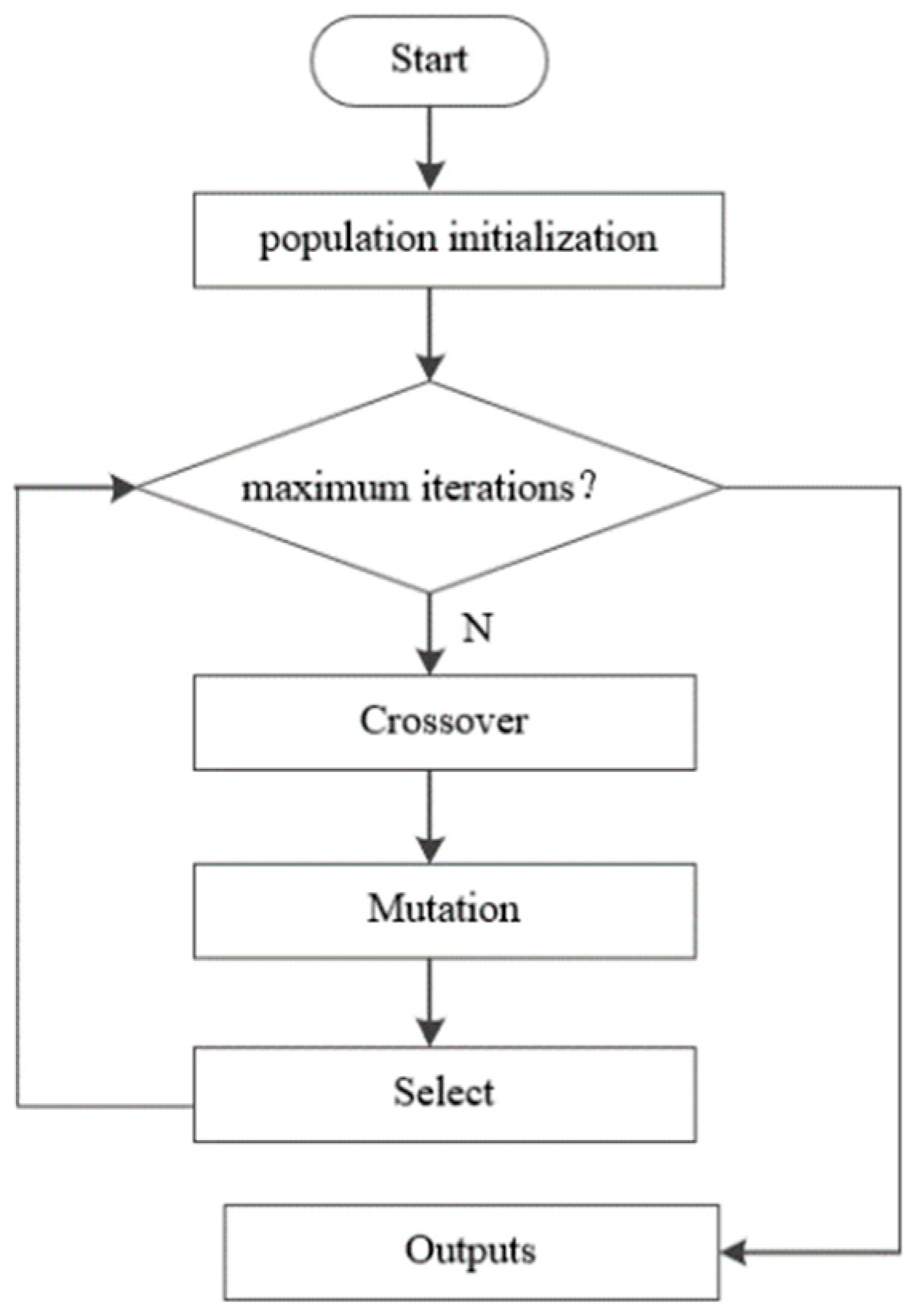
Figure 3.
Crossover.

Figure 4.
Diagram of mutation.
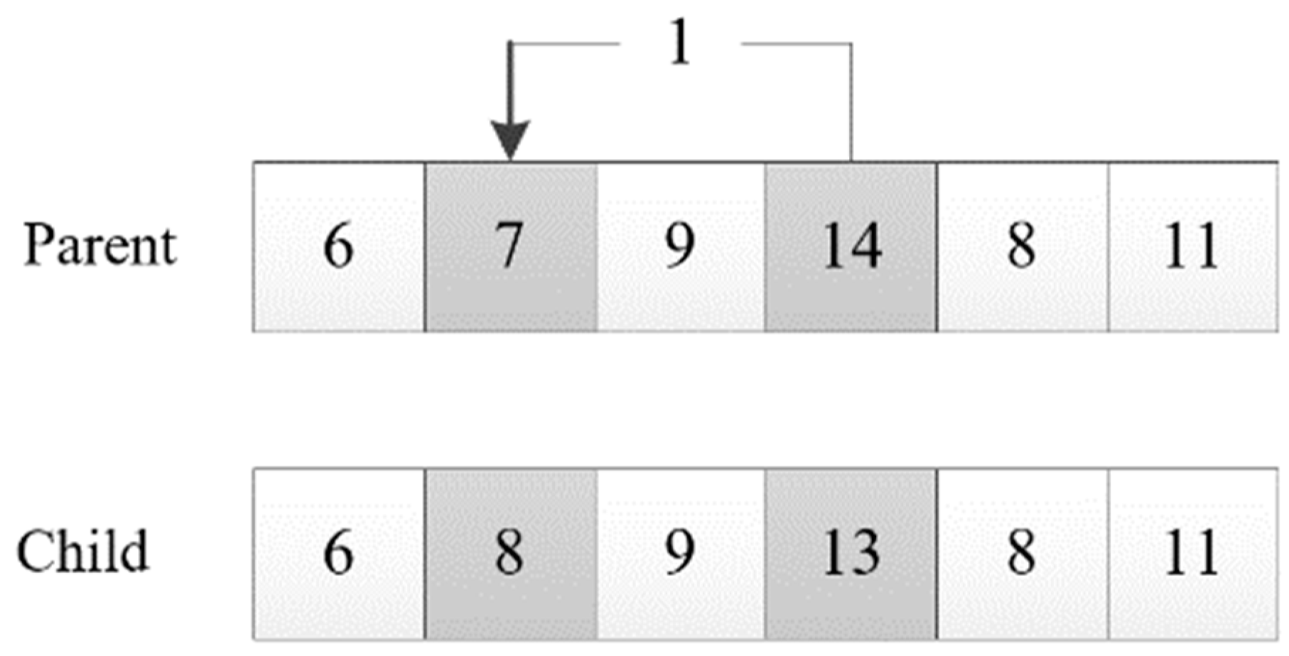
Figure 5.
Diagram of increase–decrease passenger arrival rates.
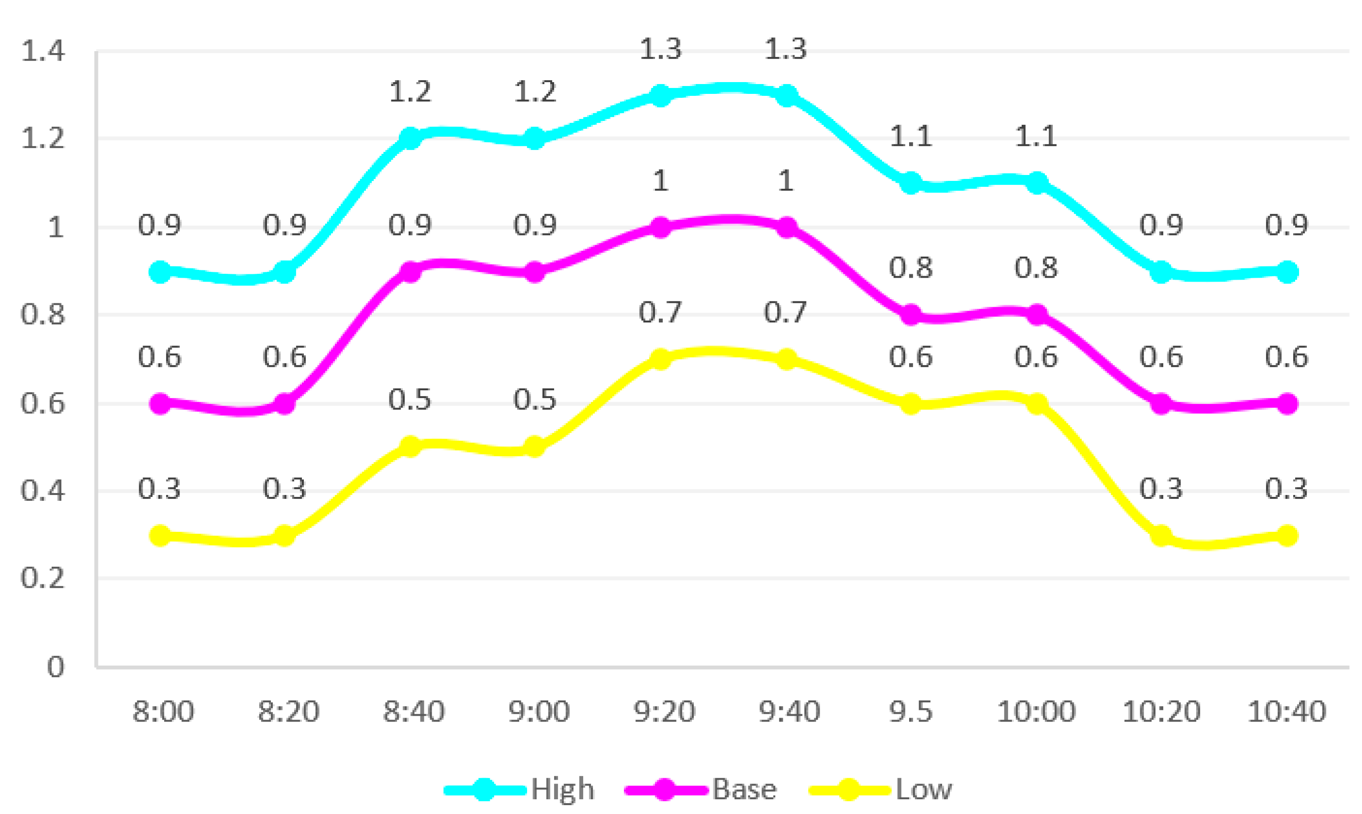
Figure 6.
Total waiting time change with the largest regret value.


Table 1.
Passenger arrival rate.
| Flow Scenario | Time | |||||||||
|---|---|---|---|---|---|---|---|---|---|---|
| 8:00 | 8:20 | 8:40 | 9:00 | 9:20 | 9:40 | 9.50 | 10:00 | 10:20 | 10:40 | |
| High | 0.9 | 0.9 | 1.2 | 1.2 | 1.3 | 1.3 | 1.1 | 1.1 | 0.9 | 0.9 |
| Base | 0.6 | 0.6 | 0.9 | 0.9 | 1.0 | 1.0 | 0.8 | 0.8 | 0.6 | 0.6 |
| Low | 0.3 | 0.3 | 0.5 | 0.5 | 0.7 | 0.7 | 0.6 | 0.6 | 0.3 | 0.3 |
Table 2.
Headway results.
| Results | Headway (Min) |
|---|---|
| Robust optimization results | 10 10 10 8 9 9 11 13 |
| Stochastic programming results | 10 10 10 8 9 8 10 15 |
Table 3.
Passenger waiting time.
| Scenarios | Optimal Solution Corresponding to the Total Waiting Time | Robust Optimization Solution Corresponding to Total Wait Time | Stochastic Optimization Solution Corresponding to Total Wait Time |
|---|---|---|---|
| Low passenger flow | 3184.99 | 3573.11 | 3831.44 |
| High passenger flow | 20,108.63 | 21,527.16 | 21,207.36 |
| Base passenger flow | 8406.08 | 8943.33 | 8907.29 |
Table 4.
Changing the maximum regret value.
| w | Total Waiting Time | Addition of the Total Waiting Time (%) | Reducing of the Maximum Regret (%) | |
|---|---|---|---|---|
| 1 | 0.23 | 11,582.14 | - | - |
| 2 | 0.20 | 11,585.81 | 0.03% | 13.0% |
| 3 | 0.17 | 11,585.81 | 0.03% | 26.1% |
| 4 | 0.13 | 11,644.43 | 0.32% | 43.4% |
| 5 | 0.10 | 11,668.62 | 1.04% | 56.5% |
| 6 | 0.07 | 11,733.16 | 1.15% | 69.6% |
Table 5.
Comparison of robust optimization and stochastic optimization.
| Zω* | Zω-ro | Zω-sp | Ws-d(%) | Wr-d(%) | |
|---|---|---|---|---|---|
| Low passenger flow | 3184.99 | 3452.29 | 3831.44 | 16.9% | 7.7% |
| High passenger flow | 20,108.63 | 21,652.20 | 21,207.36 | 5.2% | 7.1% |
| Base passenger flow | 8406.08 | 8965.01 | 8907.29 | 5.6% | 6.2% |
| Average value | 10,566.57 | 11,356.5 | 11,315.36 | - | - |
| Percentage increase | - | 7.0% | 6.6% | - | - |
| Standard deviation | - | - | - | 5.42% | 0.62% |
Publisher’s Note: MDPI stays neutral with regard to jurisdictional claims in published maps and institutional affiliations. |
© 2021 by the authors. Licensee MDPI, Basel, Switzerland. This article is an open access article distributed under the terms and conditions of the Creative Commons Attribution (CC BY) license (https://creativecommons.org/licenses/by/4.0/).
Share and Cite
MDPI and ACS Style
Liu, Y.; Luo, X.; Wei, X.; Yu, Y.; Tang, J. Robust Optimization Model for Single Line Dynamic Bus Dispatching. Sustainability 2022, 14, 73. https://doi.org/10.3390/su14010073
AMA Style
Liu Y, Luo X, Wei X, Yu Y, Tang J. Robust Optimization Model for Single Line Dynamic Bus Dispatching. Sustainability. 2022; 14(1):73. https://doi.org/10.3390/su14010073
Chicago/Turabian StyleLiu, Yingxin, Xinggang Luo, Xu Wei, Yang Yu, and Jiafu Tang. 2022. "Robust Optimization Model for Single Line Dynamic Bus Dispatching" Sustainability 14, no. 1: 73. https://doi.org/10.3390/su14010073
Note that from the first issue of 2016, this journal uses article numbers instead of page numbers. See further details here.