Abstract
Infectious diseases and pandemics, including the COVID-19 pandemic, have a huge economic impact on cities. However, few studies examine the economic resilience of small-scale regions within cities. Thus, this study derives neighborhoods with high economic resilience in a pandemic situation and reveals their urban characteristics. It evaluates economic resilience by analyzing changes in the amount of credit card payments in the neighborhood and classifying the types of neighborhoods therefrom. The study conducted the ANOVA, Kruskal–Wallis, and post hoc tests to analyze the difference in urban characteristics between neighborhood types. Accordingly, three neighborhood types emerged from the analysis: high-resilient neighborhood, low-resilient neighborhood, and neighborhood that benefited from the pandemic. The high-resilient neighborhood is a low-density residential area where many elderly people live. Neighborhoods that benefited are residential areas mainly located in high-density apartments where many families of parents and children live. The low-resilient neighborhood is an area with many young people and small households, many studio-type small houses, and a high degree of land-use mix.
1. Introduction
1.1. Background and Purpose
As of 15 February 2021, the number of confirmed Coronavirus disease (COVID-19) cases exceeded 100 million, and the number of deaths exceeded 2.3 million [1]. The damage caused by COVID-19 is global, with its effect especially being felt in large cities. Île-de-France accounts for 34% of French cases; New York, 14.6% of American cases; Quebec, 61% of Canadian cases; Metropolitan Santiago, 70% Chilean cases; and Sao Paulo, 25% of Brazilian cases [2]. In Korea, as of 26 January 2021, cases in the Seoul Metropolitan Area accounted for 61.2% of all cases [3]. In large cities, both the number of infected people and fatalities are high. As of November 2020, several regions with the highest fatality rate are situated in metropolitan areas. Specifically, Île-de-France in France, Quebec in Canada, New Jersey in the United States (US), Stockholm in Sweden, and metropolitan Santiago in Chile recorded the highest fatality rates [2]. The fatality rates in these regions are often more than twice the national average [2]. The characteristic of large cities with many people and activities is generally advantageous. However, in a pandemic situation, it is a vulnerability. The COVID-19 pandemic is re-kindling the old debate over cities’ vulnerabilities [4] to epidemics.
As of 2018, 55.2% of the world’s population lives in cities, and 23.3% live in large cities of over one million people [5]. Moreover, the city population is expected to exceed 60% by 2030 [5]. Regarding global urbanization, the vulnerability of cities to infectious diseases is a critical issue. In particular, the incidence of infectious diseases is expected to increase due to climate change [6,7,8]. Thus, it is necessary to examine cities’ preparation, response, and adaptation methods for infectious diseases [7].
Infectious diseases affect cities in various ways. This study focuses on the economic impact of COVID-19 on cities. Unlike natural disasters such as earthquakes, floods, and typhoons that cause significant physical damage to cities, infectious diseases are well known historically for their significant social and economic impacts [9]. For instance, the Black Death completely changed the economic structure of the time [10]. Even in relatively modern times, the 1918–1920 Spanish flu had the fourth largest economic impact after World War II, World War I, and the Great Depression [11].
After 2000, the 2002–2003 SARS-COV, the 2004–2006 Avian Influenza (H5N1), and the 2012 MERS-COV had a major impact on the economy. According to studies in Hong Kong [12] and Taiwan [13], SARS-COV drastically reduced consumption demand, even in a short time. The gross domestic product (GDP) is expected to decrease by 0.2% in Korea, 0.14% in the US, and 2.42% in China due to SARS-COV [14]. H5N1, though unlikely to be transmitted to humans, poses a significant threat. The global GDP is expected to decrease by 0.7 to 4.8% or 0.1 to 0.7%, depending on whether it is transmitted to humans or not [15]. MERS-COV was mainly in Saudi Arabia, the United Arab Emirates, and Korea [16]. The economic loss due to MERS-COV in Korea was estimated to reach 11 trillion won (about USD 9.9 billion) [17].
Although the COVID-19 pandemic is ongoing, some studies examine its economic impact. Sharifi and Khavarian-Garmsir [18] found that research on the impact of COVID-19 on cities is mainly conducted in four areas: environmental quality, socio-economic impact, management and governance, transportation and urban design. Early studies on the economic impact of COVID-19 reported that city revenue, income, tourism, and small- and medium-sized businesses were significantly affected [18].
The most widely cited item for the economic impact of the epidemic is the decrease in GDP [15,19,20,21,22]. The decline in GDP can be considered to be due to the combined economic impact of the epidemic. Among the individual economic impacts of infectious diseases, the reduction in consumption is widely cited [12,13,14,23]. Temporary increases in consumption for stockpiling have been reported in the United States [24,25], but this is a limited result. Consumption declines have been reported in most countries. In EU countries, consumption expenditures declined in the second quarter of 2020 [23]. In particular, the service sector, tourism, catering, and leisure sectors are immediately affected by lockdown and social distancing [9]. Unlike past epidemics, the overall decline in consumption and the transfer of consumption to online shopping now appear together. Thus, local retailers suffer significantly. Moreover, reduced consumption and changes in consumption behavior may adversely affect tax revenue for central and local governments. In addition, the collapse of the supply chain should be noted as a major economic impact of the pandemic [26], which impacts many industries [27]. In particular, the collapse of the food supply chain has been raised at the local level as well [28]. In Korea, there were no major problems in terms of daily necessities, but a significant price increase due to the shortage of masks and hand sanitizers was evident.
Economic impacts from infectious diseases, such as the decline in consumption, are not the same regionally [18,29]. Infectious diseases inhibit the movement of people via social distancing and lockdowns, causing great damage in tourist destinations and large cities where the influx of people is vital [2,29]. Moreover, since the ratio of jobs that allow for remote work is also high in large cities [2], the economic damage to commercial business areas in large cities can be significant. Further, the negative economic impact of the epidemic is greater in areas where cities lack economic diversity [30]. Given that the impact of the epidemic varies from region to region, the OECD has also raised the importance of place-based policies [2].
Thus, to establish a place-based policy, information on regional differences in pandemic influence and characteristics of such regions should be provided. However, apart from studies on tourist cities, few studies focus on the regional effects of infectious diseases and regional characteristics. In particular, it is challenging to find studies that analyze microscopic regional units smaller than the city-scale.
Given the disastrous effects of a pandemic, post-disaster resilience in cities is garnering scholarly attention. Notably, economic resilience is crucial for cities to prepare against such black-swan events [31,32]. Despite much interest in urban resilience to COVID-19, there are few academic approaches to addressing the problem because empirical research on resilience is challenging in an ongoing pandemic. Therefore, studies mainly report or estimate the economic impact of the pandemic.
This study approaches the economic resilience of cities from the perspective of local consumption. As described above, the decrease in consumption is a common phenomenon due to infectious diseases. This study gauges regional economic resilience via how quickly the reduced regional consumption recovers.
The proportion of self-employed in Korea is 24.6%, ranking sixth among the OECD, which is very high relative to the OECD average of 16.4% and the EU average of 15.3% [33]. They mainly engage in commercial activities, such as small retail, catering, and grocery, in neighborhoods. Therefore, the self-employed are directly affected by the decrease in local consumption due to the pandemic. The number of stores closed in the second quarter of 2020 in Korea reached 103,943. Thus, the number of self-employed having employees decreased by 11.5% [34]. They mainly operate small stores with part-time jobs. Their decline means the closing of small stores and unemployment for themselves and their employees.
Even after COVID-19, new pandemics are expected [6,7,8]. Even so, research on pandemics is insufficient because no infectious disease has reached pandemic status since the 1918 Spanish flu. Therefore, it is necessary to increase insight into city resilience in a pandemic situation through COVID-19 to draw implications for improving resilience in a future crisis. While pandemics do cause socio-economic damage, they also drive positive changes [35]. Therefore, this situation should be recognized as an opportunity to institute a sustainable economic system via a comprehensive understanding of all relevant changes.
Therefore, this study derived high economic resilient neighborhoods in the Covid-19 pandemic and analyzed the urban characteristics of these neighborhoods.
1.2. Theoretical Perspective
1.2.1. Urban Economic Resilience
The concept of resilience began in the fields of psychology and ecology, spreading to various fields [36]. Earlier concepts regarding resilience emphasized how quickly the system could return to an original equilibrium state when an external shock was applied [37]. This concept focused on recovery speed, and it is called “engineering resilience” [38]. Since then, the concept of resilience has expanded further. Even if the system fails to restore equilibrium, reaching a new state of equilibrium is being accepted as recovery as well. This concept concentrates on the attainment of “ecological resilience” [39]. Subsequently, studies have emerged that define the ability to adapt to continuous change as resilience, which is called “adaptive resilience” [40,41]. These concepts of resilience are related to the end goal, which can either be to “bounce back” or acquire a “new state of being” [42]. However, there are disagreements about which concept is appropriate depending on the practitioner and the discipline [42].
Since the early 2000s, urban resilience has emerged as a major issue in urban planning [42]; it has emerged as a concern of many researchers, given the spread of global urbanization trends [43]. Urban resilience is studied in various fields of urban planning. Leichenko [31] classified the literature on urban resilience into four categories: urban ecological resilience, urban hazards and disaster risk reduction, the resilience of urban and regional economies, and promoting resilience through urban governance and institutions. The OECD proposed to measure the resilience of cities in four areas: economy, society, governance, and the environment [32]. That is, studying economic resilience is a major means of understanding the resilience of a city.
As mentioned above, the concept of resilience varies across academic domains. In this study, we measured the economic resilience of a neighborhood in terms of how quickly the reduced consumption amount in the neighborhood recovering to its pre-disaster level. In other words, we used the concept of bounce-back resilience (i.e., engineering resilience) because the declining sale of local stores is the biggest damage caused by COVID-19 in Korea. Since Korea has never implemented a forced lockdown, people have not experienced any difficulty in purchasing daily necessities. In other words, the damage to consumers caused by COVID-19 is not significant. Still, the decrease in sales and closure of businesses due to voluntary social distancing and changes in consumer preferences are serious [34]. As the proportion of self-employed individuals in Korea is high [33], the problem of diminishing sales has expanded to become an overall economic problem. Therefore, the return of local consumption to its previous level is essential in Korea.
After a sufficient period following the pandemic, it will be possible to analyze resilience from the standpoint of adaptation or achieving a new equilibrium. However, this study took the first wave and first stable period of Korea as the time range of the study. This period is short (i.e., 5 months); therefore, not enough time has passed to address ecological or adaptive resilience.
1.2.2. Urban Resilience and Urban Sustainability
Urban areas account for more than 75% of global GDP and are responsible for most energy consumption and carbon emissions [44]. In this regard, urban sustainability is closely linked to global sustainability. It is also closely related to urban resilience [45], with past studies generally finding a positive correlation between them [45,46]. In the United Nation’s New Urban Agenda [47], which discusses the future direction of cities, a positive correlation between urban sustainability and urban resilience is often mentioned. However, in an urban context, the concepts of resilience and sustainability are often misdefined, too narrowly defined, or used interchangeably [48]. In such cases, resilience and sustainability can be interpreted as having a negative correlation. For example, sustainability, narrowly interpreted as maximizing efficiency, can reduce resilience by removing redundancy [46]. Elmqvist et al. [44] proposed a new concept of urban sustainability and urban resilience to overcome these problems. According to these concepts, urban sustainability normatively sets the trajectory a city should take, and resilience implies the ability to absorb disturbances and remain functional to maintain this trajectory [44]. Therefore, urban resilience can be a means to achieve urban sustainability goals.
Regarding resilience and natural disasters, D’Adamo and Rosa [45] presented the need for research on the relationship between resilience and sustainability in natural disasters such as COVID-19. In particular, they insist that the resilience system can reduce damage from natural disasters and increase urban sustainability by investing in infrastructure to overcome such disasters [45]. In other words, with COVID-19, research on urban resilience should be used as an opportunity to increase the sustainability of both cities and the human race overall. In particular, external shocks such as pandemics can shift the trajectory toward sustainability [44] and should therefore be taken as an opening to transition to a more sustainable lifestyle [49].
1.2.3. Concept of Neighborhood
In this research, the neighborhood was considered to be a unit of study. Moreover, there is no single consensus regarding the definition of a neighborhood [50]. Baffoe [50] reviewed previous studies on neighborhood and categorized the definition of a neighborhood into three categories: neighborhood as a place, neighborhood as a community, and neighborhood as a policy unit. The neighborhood as a place denotes a locality where people reside and spend a lot of time. Consequently, people’s quality of life is greatly affected by neighborhoods [51]. Neighborhood as a community takes into account the shared beliefs and interests of people living in the neighborhood [52]. Neighborhood as a policy unit refers to a unit for implementing policies at the local level [50].
In the field of planning, the concept of neighborhood, which began with Howard’s garden city concept [53] and developed into Perry’s neighborhood unit [54], is mainly employed. According to this concept, neighborhoods are small areas where people spend their daily lives, and their physical, social, and economic characteristics directly or indirectly affect others around them [55]. This definition of a neighborhood is closest to the concept of the neighborhood as a place. In the planning field, neighborhoods are also perceived as areas where essential services are provided [56,57]. This concept links to the neighborhood as a policy unit. This study deals with the neighborhood as an area where residents’ daily consumption activities take place. Thus, the concept of a neighborhood as a place is most actively borrowed.
There have been many discussions concerning the criteria for classifying and categorizing neighborhoods, but no consensus has been achieved. The demographic composition (e.g., age, race, gender, etc.), housing-related factors (e.g., housing type, housing age, etc.), socio-economic class, physical environment, transportation, and health are frequently used as criteria for classifying neighborhoods [58,59]. For analysis, we selected related variables as urban characteristics.
1.3. Case Context
1.3.1. Changes in the Number of COVID-19 Confirmed Cases in Korea
Figure 1 shows the number of COVID-19 confirmed cases per month in 2020. In Korea, there were three waves after the first confirmed case. During the stable period after the first wave, the number of confirmed cases decreased sharply. In May, there were fewer than 25 confirmed cases per day nationwide. Accordingly, in Korea, the local economy recovered rapidly, and people’s consumption also recovered. Given such rapid recovery, Korea’s economic growth rate in the second quarter of 2020 was −3.2%, ranking first among OECD member countries. Further, this is very high relative to the OECD average (−10.5%), the EU average (−11.4%), and the US (−9%) [60].
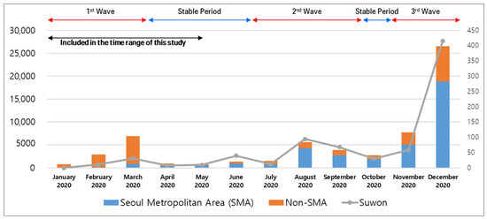
Figure 1.
South Korea’s COVID-19 new cases per month (data source: References [3,61]).
These changes make it possible to study the economic damage and recovery of cities in the situation where the COVID-19 pandemic is still ongoing. This study spanned June 2019 to May 2020, when the number of confirmed cases decreased the most, including the first wave. Moreover, the study employed consumption data for a year to confirm the usual consumption pattern.
1.3.2. Status of Suwon City
This study investigated Suwon. In Korea, cities are administratively divided into metropolitan cities and general cities. Since this study conducted a neighborhood-level analysis, we posited that metropolitan cities with large commercial catchment areas were not appropriate. Moreover, this study analyzed the economic impact of large cities vulnerable to pandemics. Suwon has a population of 1.23 million [62], making it the most populous among general cities in Korea.
Further, since this study employed credit card payments as consumption data, cities with online-shopping companies are unsuitable for analyses, because online shopping payments are counted as sales at such locations. Therefore, Seoul, with 83.1% of Korea’s major online-shopping companies, and Seongnam, with 7.7% [63], are unsuitable for the study. Suwon has no major online-shopping company; thus, the amount of card consumption in Suwon was used at offline stores.
Figure 2 shows the location and topography of Suwon City. It is located in Gyeonggi-do, with an area of 121.09 km2 and a population density of 10,115 people/km2. A mountain is located in the north of Suwon, and agricultural land is preserved in the west. At the south, there is an airbase, which is expressed as agricultural land.
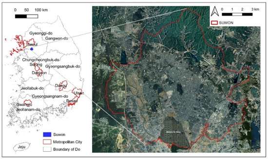
Figure 2.
Location and satellite image of Suwon.
During the second half of 2019, the employment rate in Suwon city was 60.2%, which is lower than the national average (i.e., 60.9%) and the average employment rate of Gyeonggi-do (i.e., 61.9%) [64]. Conversely, in 2018, the ratio of manufacturing workers in Suwon City was 10.7%, which is less in comparison to Gyeonggi-do (25.5%) [65]. On the other hand, the ratio of workers in the professional service industry was 12.4%, which was larger in contrast to Gyeonggi-do (i.e., 5.0%) [65]. In sum, Suwon is a city with a smaller manufacturing sector and a larger service sector, as opposed to other cities in Gyeonggi-do. Moreover, the ratio of accommodation and food service, which are industries vulnerable to COVID-19, is 11.2%, which is greater than in Gyeonggi-do (i.e., 9.7%) [65].
1.3.3. Suwon’s Consumption Reduction and Recovery in the COVID-19 Pandemic
Consumption declined significantly due to the outbreak of COVID-19 in Korea but recovered rapidly after the first wave subsided. Figure 3 shows the change in credit card payments in Suwon and the number of COVID-19 confirmed cases in Korea within the study period. The line graph shows the amount of card payment in Suwon, and the bar graph shows the number of new COVID-19 cases. The gray dotted line represents the average value of the card payment for the seven months (June 2019 to December 2019) before the occurrence of COVID-19.
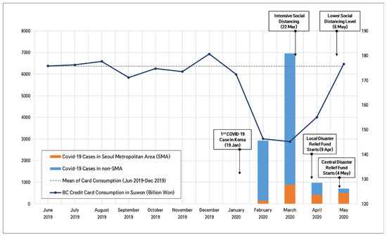
Figure 3.
Korea’s COVID-19 cases per month and credit card payment amount in Suwon (data source: References [3,68]).
After the first case in January, the amount of credit card payments decreased sharply. In March, when the payment amount was the lowest, the number of cases was the highest, and intense social distancing began. In response to the rapid decline in consumption, the central and local governments began to pay the Disaster Relief Fund (DRF). In Suwon, from 9 April, the local government paid 100,000 won per person [66]. From 4 May, the central government’s paid 1 million won for a family of four [67]. The DRF can be used within the local area and cannot be used for online shopping. Accordingly, local consumption recovered rapidly. Moreover, in May, the consumption of Suwon recovered to a normal level. On May 6, the Korean government lowered the level of social distancing, allowing citizens to return to their daily life. Such changes are typical shock-and-recovery patterns in disaster situations. Thus, the temporal range of this study is appropriate to analyze the resilience of the pandemic.
1.4. Research Question
This study began with the awareness of the problem that consumption reduction and recovery are not the same in all neighborhoods. The overall consumption of Suwon showed a pattern of decreasing and recovering. However, there were different patterns for each neighborhood. In a pandemic situation, consumption in some neighborhoods recovers quickly (slowly). Some neighborhoods have high economic resilience relative to other neighborhoods. The first research question is as follows: what are the urban characteristics of high-economic-resilient neighborhoods in a pandemic situation?
Further, after the outbreak of COVID-19, consumption did not decrease but increases continuously in some neighborhoods. Such neighborhoods benefit economically in a pandemic situation. The second research question is as follows: what are the urban characteristics of neighborhoods that benefit economically in a pandemic situation?
2. Materials and Methods
2.1. Research Method
Figure 4 presents the analysis method. First, the neighborhood types are classified by analyzing the change in the credit card payment by neighborhood. The neighborhoods are classified into low-resilient neighborhoods, high-resilient neighborhoods, and benefited neighborhoods. The specific classification method is reported in Section 2.3.
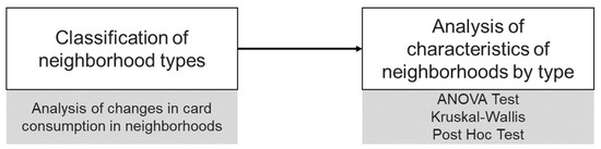
Figure 4.
Research method.
ANOVA (Analysis of Variance) and Kruskal–Wallis (K–W) tests were utilized to assess urban characteristics for each classified neighborhood type. Thereafter, post hoc testing was performed to confirm the significance of the difference between each type. When a variable satisfied the normality, a parametric test method (i.e., ANOVA) was used, and when the normality was not satisfied, a non-parametric test method (i.e., K–W) was utilized. For variables using ANOVA, Levene’s equal variance test was performed. For variables with equal variance, F statistic was used in the ANOVA, and the Scheffe method was used in the post hoc. For variables not satisfying the equal variance, the Welch statistic was used in the ANOVA, and the Games–Howell (GH) method was used in the post hoc. Further, for the variables using the K–W test, we adopted Dunn’s method during post hoc analysis.
2.2. Data Construction
2.2.1. Selection of Neighborhoods to Be Analyzed
This study employed the Bank and Credit (BC) credit card payment data in the neighborhood to determine the consumption amount by neighborhood. In Korea, credit card payments represent local consumption [69]. The share of credit card usage in Korea’s total consumption was 53.8% as of 2019 [70], and BC Card’s credit card market share was 24% [66]. Therefore, the BC Card payment amount is expected to represent the overall consumption behavior. Nevertheless, if there is a large difference in user characteristics depending on the card company, there is a possibility that the payment amount data of the BC card may not represent the total consumption. Therefore, caution is mandated in the use of research results.
The card payment data used in this study were collected in units of Output Area (OA). An OA is the smallest spatial unit for collecting statistical data in Korea and is set based on population size, socio-economic homogeneity, and boundary shape [71]. It is set per 500 people, and socio-economic homogeneity is set per housing type and land price [71]. An OA is a neighborhood where about 500 people with similar socio-economic characteristics live.
Since the population size is the most important criterion for setting an OA, the OA of mountains or farmlands is very wide. Figure 5 shows Suwon’s OAs and land-use area. The OAs of green areas are vast relative to other OAs. It is challenging to consider such large OAs as neighborhoods. Thus, we excluded OAs with an area of 100,000 m2 or more from the analysis.
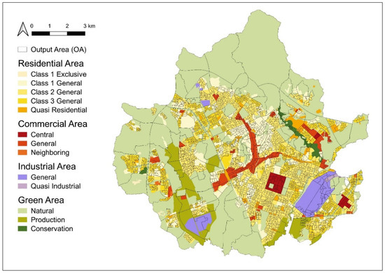
Figure 5.
OA boundary and land-use zone of Suwon.
This study addresses consumption in neighborhoods. Therefore, OAs for which card payments do not exist were also excluded. If the card payment data do not exist, and there are no stores or restaurants, the OA can be considered as comprising only residential building. Further, even if card payment data exist, an OA with a small number of payments is considered a neighborhood consisting mostly of houses. Therefore, we also excluded OAs with less than 5000 payments per year from the analysis. This study uses building-related data as a major urban characteristic variable. Therefore, OAs for which no building data exist were also excluded.
Hence, 846 OAs were included in this study. The OA derived through this process has a population of about 500, with residential and commercial facilities. Figure 6 reports the OAs included in the study. All large OAs, including green areas, were excluded, and some OAs in industrial and commercial areas were excluded. The area average of OA included in this study was 25,870 m2, and the population average was 483.6.
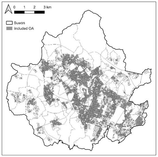
Figure 6.
OAs included in this study.
2.2.2. Variables and Data Source
Since the economic impact of the pandemic has been studied mainly on macroeconomic factors such as GDP, the urban characteristics of neighborhoods regarding the economic impact are not well known. Therefore, we selected basic variables representing city characteristics as analysis variables. Moreover, these variables are well-known criteria for the classification of neighborhoods [58,59]. Table 1 summarizes the study variables. In the process of data construction, when analysis and calculation of spatial data were required, the Quantum Geographic Information System (QGIS) 3.10 was used.

Table 1.
Urban characteristic variables.
First, in the demographic category, the population ratio by age was selected to know the age groups that live in the neighborhood. Notably, the changes in behavior patterns in pandemic situations differ per age. Migration for those aged 20 and over 70 decreased significantly more than it did for those in their 30s and 50s [72]. Changes in consumption patterns also differ per age, with the smallest decrease among those in their 50s [72].
The household structure was employed to ascertain what household type lives in the neighborhood. It comprises variables that can determine the number of household members living in one house (HH-M), variables that can determine the generation of family members living together (HH-1G, HH-2G, and HH-3G), and the ratio of non-related households (HH-NR) as the analysis variable.
Housing-related variables are divided into housing size and type. Through the size of the house, it is possible to check the income level in the area. The type of house is the main variable that determines the characteristics of the neighborhood. A specific housing type often dominates one OA.
Data provided by the Statistical Geographic Information System (SGIS) [73] operated by the Statistics Korea (national statistical agency) were used for the demographic, household structure, and housing-related variables. SGIS provides the population by age, the number of households by type, the number of houses by area, and the number of houses by type (i.e., aggregated in OA), which is the analysis unit of this study. We created proportion variables that divided these parameters according to the total population, the total number of households, and the total number of houses.
The proportions of building floor area by use and land-use mix variables were selected as land-use-related variables. The former was divided into residential, commercial, and educational or cultural. These uses are the most representative in the city.
Land-use mix notably affects the volume of pedestrians and vitality in a region. Several studies in urban planning have repeatedly confirmed that as the land-use mix increases, the volume of pedestrians increases [74,75,76,77], which leads to an increase in local consumption [78,79,80]. Among the various variables for measuring land-use mix, this study selected three variables. The number of uses (No-U) checks the diversity of uses. Diversity has been known to significantly influence regional vitality since Jacobs [81]. The Hirschman–Herfindahl Index (HHI) and the Residential and Non-Residential Balance Index (RNR) were included as indicators to determine the degree of the land-use mix. HHI is widely used to measure market concentration in the economic field [82,83]; it is also widely used as a variable to measure the land-use mix [84,85,86,87]. HHI is calculated via Equation (1). It is 1 for single-use and 1/k when k uses are uniformly mixed. Therefore, the smaller the HHI value, the greater the degree of the land-use mix.
In the above equation, K is the number of use, and is the proportion of floor area of use (i).
RNR is measured by using Equation (2). It measures the degree of land-use mix simply by dividing the use of a building into two types: residential and non-residential. RNR is 0 for single-use and closer to 1 when residential and non-residential are mixed. That is, the greater the RNR, the greater the degree of the land-use mix.
In the above equation, R is the floor area of residential buildings, and NR is the floor area of non-residential buildings.
The National Spatial Information Portal [88] provides shape (SHP) files that specify the location and shape of buildings. This file elucidates the use and floor area of each building. We utilized this data to calculate the total floor area according to use and the number of uses for each OA. The variables of the use of building and land-use mix categories were calculated by using this data.
The transportation-related variables were selected as the ratio of road area (RD), distance to the nearest railway (or subway) station (TR), and bus stop density (BUS). RD captures the convenience of using a car. To formulate this variable, the road area was calculated by using the road SHP file provided in the National Spatial Information Portal [88]. Afterward, the road area was derived and divided by the OA.
TR is railroad or subway accessibility. For this variable, SHP files of subway stations and railway stations provided by the Ministry of the Interior and Safety [89] were selected. The straight-line distance from the center point of OA to the nearest subway station or railway station was calculated.
BUS addresses the convenience of using the bus. This variable used the bus stop coordinate data provided by Gyeonggi Data Dream [90]. The location of bus stops was geocoded, and the number of bus stops in OA units was counted.
Population density (DN-P) and building density (DN-B) variables were selected as density variables. DN-P used population density data of the OA provided by SGIS [73]. DN-B was calculated by dividing the total building area calculated earlier by the OA.
2.3. Classification of Neighborhoods
The resilience triangle is widely used to quantitatively measure engineering resilience. Bruneau et al. [91] presented a concept for quantitatively measuring the resilience of infrastructure against earthquakes. Figure 7 shows that after the earthquake, the performance of the infrastructure drops sharply relative to the normal and recovers after a certain period. Bruneau et al. [91] quantitatively defined the resilience, as shown in Equation (3) in this situation, which is the same as the area of the part shaded blue in Figure 7. Thus, the part at the top of the graph can be judged as the degree of damage caused by the disaster; it is known as a resilience triangle.
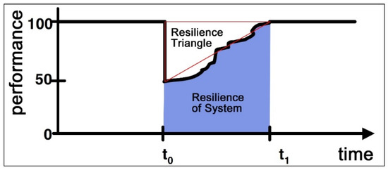
Figure 7.
Conceptual definition of resilience (modified from Bruneau et al. [91]).
The concept of the resilience triangle was used to measure resilience in many prior studies [92,93,94,95]. The shape of the resilience triangle can vary depending on the analysis target and impact type. Balal et al. (2019) suggested the concept of a resilience polygon because the resilience triangle can appear in various shapes, such as right triangle, acute triangle, trapezoid, pentagon, and hexagon [92].
Following the concept of the resilience triangle, the concept of high resilience can be derived. Figure 8a shows that the size of the resilience triangle is determined by the degree of damage and the time it takes to recover. Moreover, the degree of damage is related to the system robustness, and the time taken to recover is related to the speed of recovery. A system with robustness and fast recovery has less disaster damage and a short recovery time. Such a system can be judged as a high-resilient system [91,96,97]. In other words, a system with a small resilience triangle has high resilience.

Figure 8.
(a) Determinants of resilience triangle. (b) High- and low-resilient system.
Figure 8b is a schematic diagram of this concept. The resilience triangle ABC of the high-resilient system, indicated in blue, is smaller than triangle ADE of the low-resilient system, indicated in red. The area of a triangle can be easily calculated by knowing the lengths of AC, AE, FB, and FD. The length of FB and FD can be determined by the performance level at the time of the greatest damage. In other words, , representing the robustness of the high-resilient system, is larger than of the low-resilient system. Thus, it maintains a relatively high performance level even in the event of a disaster, with minimal damage. Since the pandemic is not over, it is difficult to ascertain the length of AC and AE, the time taken to recover to previous levels. Therefore, we judged the recovery speed through the degree of recovery at a specific time point after the COVID-19 outbreak. The recovery speed can be determined based on the performance level at the point after a certain time has passed since the disaster occurred. The recovery degree () of the high-resilient system can be expected to be larger than that () of the low-resilient system.
Unlike natural disasters, such as earthquakes, the economic shock caused by the pandemic did not damage all neighborhoods. In a pandemic situation, people are reluctant to use large stores or central commercial areas that are over-crowded, thereby reducing overall consumption. Simultaneously, essential consumption usually occurs in areas close to residences. Therefore, in certain neighborhoods, consumption may not decrease comparatively but does tend to increase. As shown by the green line in Figure 8b, after a disaster, consumption in a neighborhood continues to increase more than the usual level. Such neighborhoods may be construed as having benefited economically from the pandemic. Accordingly, three neighborhood types emerge: high-resilient (HRN), low-resilient (LRN), and benefited (BFN) neighborhoods.
In this study, credit card payments in neighborhoods were used as variables to measure economic performance in a pandemic situation. However, the level of credit card payment varies per neighborhood. Therefore, a comparative indicator is necessary. From Equation (4), we used the mean value of card payments for each OA from June 2019 to December 2019 before the COVID-19 outbreak as the usual payment amount for the corresponding OA(. From Equation (5), the monthly card payment amount ( was then divided by the usual payment amount ( and used as an indicator ( to determine the level of payment relative to the usual monthly payment amount. If the value of indicator ( is less (greater) than 1, consumption decreased (increased) in the neighborhood than usual. If we can obtain the usual payment data for a specific month for each OA(, it is ideal to standardize by using this mechanism. Nonetheless, we used because only one year’s data can be used from June 2019 to May 2020.
indicate the consumption level in “i” neighborhood from January to May 2020 after the COVID-19 outbreak. We set as greater than 1 regarding the BFN. They are neighborhoods where the level of consumption in the neighborhood has not decreased at all since the COVID-19 outbreak.
After classifying BFN, HRN and LRN were categorized for the remaining neighborhoods. The , derived through Equation (6), represents the consumption level when the damage of COVID-19 was greatest in the neighborhood. This value has the same meaning as the “d” value in Figure 8b. Within the sample period, the consumption level in the last period of May 2020 is , which has the same meaning as “r” in Figure 8b.
We classified the neighborhood in which the values of “d” for robustness and “r” for the degree of recovery fall in the top 30% as HRN. They are highly robust. Thus, the degree of damage is small, and the degree of recovery is high. Of course, these neighborhoods can be expected to have a small resilience triangle. Therefore, the low resilience of LRN is a relative concept to HRN.
3. Result
3.1. Result of Neighborhoods Classification
Based on the method described in the previous section, the OAs in Suwon were classified into three types: 130 BFN, 111 HRN, and 605 LRN. Figure 9 shows the change in the mean value of the consumption indicator (for each neighborhood type. The results of all neighborhoods (shown in gray) show a pattern similar to the change in total sales (Figure 3). However, the results divided by type show very different patterns.
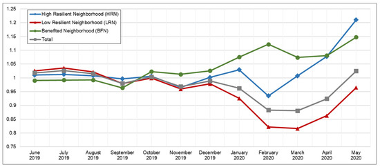
Figure 9.
Changes in consumption indicator ( by neighborhood type.
The BFN (the green line) increased after the COVID-19 outbreak. The HRN (the blue line) shows a decrease in February but starts to recover quickly, showing a higher recovery than BFN in May. Thus, resilience is high. The LRN (red) has a greater degree of damage and slower recovery than the HRN. This result conforms to the conceptual diagram in Figure 8b.
Figure 10 shows the spatial distribution of divided neighborhoods. The BFN and HRN are not concentrated in a specific area and are distributed spatially evenly. Thus, the high resilience of neighborhoods is not due to locational features in the level of urban spatial structure. However, it can be understood that economic resilience varies per the internal characteristics of individual neighborhoods.
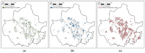
Figure 10.
Spatial distribution of neighborhood by type: (a) benefited neighborhood (BFN), (b) high-resilient neighborhood (HRN), and (c) low-resilient neighborhood (LRN).
3.2. Urban Characteristics by Neighborhood Type
3.2.1. Demographic Characteristics
Table 2 shows the results of the ANOVA test for demographic variables. According to Levene’s test result, if the variance was equal, the F statistic was reported. In the case of not equal variance, the Welch statistic that can be used when the assumption of equal variance is not satisfied is reported. For variables other than P-50, there is a statistically significant difference in mean values between neighborhood types.
Table 2.
ANOVA test results of demographic variables.
Figure 11 reports the mean value of the variables by group. In the figure, the number of stars under the variable name indicates the statistical significance of the ANOVA or K–W test. Table A1 reports descriptive statistics, including the mean value of each variable by type. Table A2 reports the results of the post hoc test, which can check the statistical significance of the difference in the mean value of the variable between each neighborhood type. Regarding (not) equal variance, the (GH) Scheffé method was used. Refer to the results of Table A1 and Table A2 for the interpretation of the text.
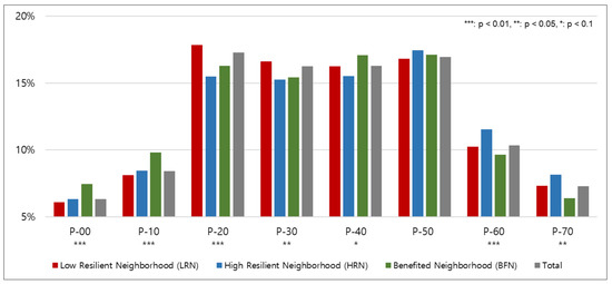
Figure 11.
Mean difference of demographic variables by type.
P-00 mean value of the BFN is statistically larger than that of the LRN. In P-10, the value of the BFN is significantly greater than that of the LRN and HRN. Thus, more adolescents and children live in the BFN than in other neighborhoods. At P-20, the mean value of the LRN is statistically greater than the HRN. The mean P-30 of the LRN is statistically greater than that of the HRN and BFN. Thus, the LRN is a neighborhood where more young people in their 20s and 30s live than in other neighborhoods. Looking at P-40, the BFN has a larger value than the HRN, which is linked to the results of P-00 and P-10. In the BFN, children and adolescents often live with their parents. There was no statistically significant difference in P-50 between groups. P-60 represents a higher value for the HRN than for the LRN and BFN. In P-70, the HRN shows a higher value than the BFN. HRN is a neighborhood with more elderly aged 60 or older than other neighborhoods.
3.2.2. Household Structure Characteristics
Table 3 shows the results of the ANOVA test of variables related to household structure. The Welch statistic result was reported because all variables did not satisfy the assumption of equal variance. Except for HH-1G, the other variables had statistically significant differences in mean values between neighborhood types.
Table 3.
ANOVA test results of household structure variables.
Figure 12 reports the mean values for each type. The mean of HH-M was significantly greater in the BFN than in the HRN and LRN. That is, the number of member of households living in the BFN is higher. HH-1G and HH-3G had no significant difference between groups. In HH-2G, the mean value of the BFN is significantly higher than that of the LRN and HRN. Overall, the BFN has more of two generations of parents and children than other neighborhoods. The HH-1P mean of the BFN is smaller than that of the LRN and HRN. Thus, there are fewer single-person households in the BFN. The mean value of HH-NR in the LRN is significantly larger than that of other types. Hence, in the LRN, many households comprise non-family people. Considering the results of the demographic variables, many young people live with roommates in the LRN.
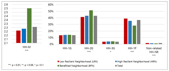
Figure 12.
Mean difference of household structure variables by type.
3.2.3. Housing-Related Characteristics
By examining the normality of housing-related variables employing the Q–Q plot, it is evaluated that the housing-related variables do not satisfy the normality. Correspondingly, K–W analysis, a non-parametric test, was performed (refer to Table A3 for the Q–Q plot of the variables). Table 4 reports the results of the K–W analysis of housing-related variables. It is divided into two categories: housing-area and housing-type variables. There were statistically significant differences between groups except for HS-4, HS-5, and HT-R. For HS-1, HS-3, and HT-M, the K–W test was significantly analyzed, but there was no significant difference between groups in the post hoc test.
Table 4.
Kruskal–Wallis test results of housing-related variables.
Figure 13 and Figure 14 report the difference in the mean value of each type of housing-related variable. The HS-2 mean value of the LRN is statistically larger than that of the BFN. In the case of HS-1, it is not statistically significant, but the value of LRN is the largest. That is, the proportion of small houses in the LRN is larger than that of other neighborhoods.
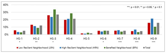
Figure 13.
Mean difference of housing-size variables.
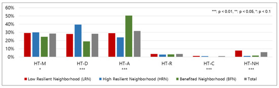
Figure 14.
Mean difference of housing-type variables.
As for the values of HS-4 and HS-5, the BFN is very large. Therefore, BFN can be thought of as an area with many middle-sized houses, but it is not statistically significant; hence, the findings should be interpreted with care.
Regarding the mean value of the HS-7, HS-8, and HS-9 variables, representing the proportion of large-sized houses, the value of the HRN is significantly larger than that of the LRN and BFN. Hence, the HRN has more large-sized houses than in other neighborhoods.
In summary, there are more small (large) houses in the LRN (HRN) than in other neighborhoods. Further, in the BFN, there are more middle-sized houses relative to other neighborhoods.
The value of HT-D, the proportion of detached houses, is the highest in the order of HRN, LRN, and BFN. That is, the HRN is a neighborhood with many large detached houses.
The value of HT-A, the apartment ratio, is significantly larger in the BFN than in the HRN and LRN. That is, the BFN is an area with many apartments.
The values of HT-C and HT-NH are higher in the LRN than in other neighborhoods. It means many living quarters in the LRN use studio-type houses or commercial buildings.
3.2.4. Land-Use Related Characteristics
Table 5 shows the results of the ANOVA and K–W test of variables related to land-use. All variables have significant mean differences between groups. Figure 15 shows the mean difference between groups.
Table 5.
ANOVA or K–W test results of land-use related variables.
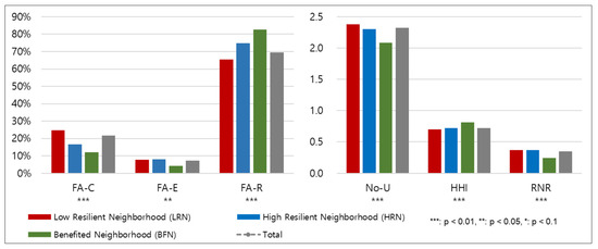
Figure 15.
Mean difference of land-use related variables.
Regarding the floor area proportion of commercial buildings (FA-C), the LRN was the largest, followed by the HRN and BFN. However, for residential use (FA-R), BFN was the largest, followed by HRN and LRN. For educational and cultural uses (FA-E), the LRN value was larger than that of the BFN. The LRN (HRN and BFN) has (have) relatively many commercial (residential) buildings.
Similar results were also found for variables related to the land-use mix. In No-U, the value of the LRN is significantly larger than that of the BFN. The higher the HHI value, the more it is centered on single use. Further, the degree of the land-use mix is lower. The HHI value of the BFN was significantly higher than that of other neighborhoods. The smaller the RNR value, the smaller the degree of the land-use mix. The value of the BFN was also smaller than that of the other neighborhoods. Therefore, the BFN was mainly for residential purposes, with few other uses.
3.2.5. Transportation Characteristics
Table 6 reports the results of the ANOVA test for traffic-related variables. Figure 16 reports the mean value for each neighborhood type. There is a statistically significant difference between groups in RD and BUS, and there is no significant difference in TRN. The RD value of the BFN is statistically and significantly smaller than that of other neighborhoods. Hence, the proportion of apartments in the BFN is high. Since Korean apartment complexes are often large complexes that occupy the entire block, the road area ratio is considered low.
Table 6.
ANOVA or K–W test results of transportation variables.
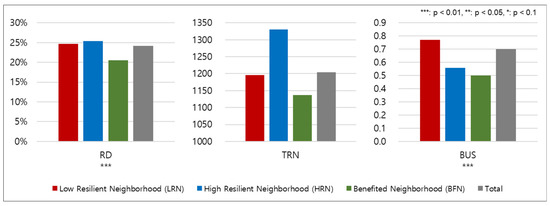
Figure 16.
Mean difference of transportation variables.
The BUS value of the LRN is significantly greater than that of other neighborhoods. There are relatively many commercial buildings in the LRN. Therefore, access to public transportation is considered better.
3.2.6. Density Characteristics
Table 7 reports the results of the K-W test of the density-related variable. Figure 17 reports the mean value for each neighborhood type. There are differences between groups in both population density and building density. The population density is higher in the BFN than in other neighborhoods. Accordingly, many apartments are high-density houses in the BFN.
Table 7.
Kruskal–Wallis test results of density variables.
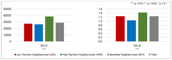
Figure 17.
Mean difference of density variables.
The building density is statistically lower in the HRN than in other neighborhoods. The HRN result is similar to the previous analysis, which derived a low-density residential area mainly for detached houses.
4. Discussion
Table 8 summarizes urban characteristics by neighborhood type per the results of this study. Thus, it is possible to check the characteristics of the HRN and BFN in a pandemic. Moreover, the characteristics of the LRN, where recovery is slow, are evident.
Table 8.
Urban characteristics according to neighborhood type.
First, the HRN is home to many senior citizens, with more large-scale detached houses than other areas. Regarding land-use, it is situated between the LRN and BFN. That is, commercial and residential are properly mixed. There are many low-rise detached houses in HRN, with low density. Hence, the HRN is a low-rise mixed-use area where many elderly people with relatively high incomes reside. Consumption in such neighborhoods decreased at the start of the COVID-19 outbreak but recovered rapidly after the initial shock due to the low online shopping accessibility and mobility among the elderly. The online-shopping usage rate among those in their 20s (96.9%) and 30s (92.4%) is very high compared to the overall average (i.e., 64.1%) [98]. Contrariwise, online-shopping use rates of individuals in their 50s (44.1%), 60s (20.8%), and 70s (15.4%) are very low [98]. During a pandemic, such a large difference in accessibility to online shopping seems to induce a difference in neighborhoods’ consumption patterns.
The BFN has a large population of minors, and many households comprised parents and children. Moreover, it has mainly high-density apartments, and the ratio of residential use is higher than in other neighborhoods. Such an area is a high-density residential area where large families, including children, live together. Residents of such neighborhoods normally shop in large commercial facilities away from their residence. However, during the pandemic, preference for large commercial facilities where many people gathered decreased. Accordingly, consumption near homes seems to have increased. Apparently, consumption did not decrease even in the early stages of the COVID-19 outbreak, as a large amount of essential consumption catered for children and adolescents. This change in consumption patterns can be viewed as positive: increasing consumption in small local shops can lead to higher consumption of locally produced goods, increasing the likelihood of a transition to a circular economy [35].
Relative to other neighborhoods, the LRN has more commercial buildings, a mixture of various uses, and many young people. There are many studio-type small houses, with many cases of non-family members living together. Such an area is usually the most vibrant in the city, given the many young people and commercial and social activities. However, during the pandemic, such regions were found to have relatively low resilience. Younger generations have quickly transitioned to online consumption due to the ease of access to (and comprehension of) online shopping. Further, the recovery in these regions was slow due to a significant decrease in social activities from social distancing. Since this study uses the concept of engineering resilience, this situation was deemed as low resilience. However, if we apply the concept of adaptive resilience, a new equilibrium is apparent. Additionally, the youth rapidly adopt new consumption behaviors to maintain their quality of life and are likely to maintain a new way of life even after the pandemic. Still, from the perspective of local merchants, it is unreasonable to see this situation as a new equilibrium. They suffer greatly from the decline in sales, and their survival is compromised.
The study findings have the following implications for urban planning. First, urban characteristics that enhance urban vitality in general situations, such as youth population, various social activities, and land-use mix, can be disadvantageous in a pandemic because it is easy for young people to move their consumption online, and social activities are greatly restricted. The results are similar to those of city-scale studies that show that metropolitan areas and tourism-centered cities suffer a great deal of economic damage from infectious diseases. In a situation where the cycle of infectious diseases is expected to be short in the future, it is necessary to reexamine the existing common sense in urban planning. To overcome such a situation, urban planning with a reinforced social-mix concept should be implemented. In Korea, social-mix has aimed to mix income classes. However, considering the results of this study, a social mix wherein various ages and households can be grouped into neighborhood units should be conducted.
Second, experiences in pandemic situations may have a positive effect in the long term. In Korea, the problem of local retail stores closing due to their inability to compete with large commercial facilities has been noted. In a pandemic situation, as the preference for large-scale commercial facilities declines, consumption in local retail stores around residential areas is emerging. Accordingly, the BFN emerged. Simply put, the possibility of change to sustainable consumption behavior through experiences in pandemic situations is suggested. If the local consumption experience continues during the pandemic, long-term consumption preferences of consumers may change. Of course, local retail stores must also improve their competitiveness. To induce such a positive change, more active dissemination of local currency should be considered. In Korea, local currency can only be used in the local area but cannot be used in large commercial facilities. Hence, the spread of local currency can increase the positive local consumption experience. It is also possible to provide the DRF only in the local currency, and various incentives to facilitating the use of local currency can be presented in a pandemic situation.
Third, it is necessary to supply urban infrastructure for each neighborhood living area. As seen in the case of HRNs and BFNs, in a pandemic situation, people have the potential to shift their activities of everyday life, such as consumption, to the neighborhood around their homes, and there is a need for efforts from the public sector to sustain and strengthen such positive changes. Green spaces, such as small parks and children’s playgrounds, can be important infrastructure for increasing activities in the neighborhood. In particular, it was confirmed that open space plays a key role as leisure space for citizens during a pandemic. The expansion of urban green spaces will strengthen urban resilience and sustainability [45] and increase local activities to help introduce sustainable consumption behaviors such as circular consumption [35].
Fourth, the elderly’s digital literacy needs to be supported. In HRNs, consumption recovered rapidly, which could be due to the elderly’s low accessibility to online shopping. However, in the long run, seniors’ access to online shopping and delivery apps needs to be improved. D’Adamo and Rosa [45] proposed embracing digitalization for urban sustainability and resilience after the pandemic. In Korea, public support is needed to improve access to digital consumption, especially for the elderly. To this end, the Korean government recently launched a public delivery app [99] and is pursuing digitalization of infrastructure and strengthening of the digital access of vulnerable groups such as the elderly through the Digital New Deal policy [100,101].
This study on the economic resilience of small regions in a pandemic is rare and significant. In particular, the urban characteristics of regions with high resilience can be used as basic data for future urban planning in preparation for the next potential pandemic. However, this study has limitations as follows. First, the long-term effects could not be analyzed. This study includes only the first wave and stable period in Korea. Since then, there have been second and third waves. Moreover, the pandemic is ongoing. It is challenging to understand the resilience and characteristics of neighborhoods in a situation where the pandemic and social distancing persist. Therefore, studies on the long-term impact and resilience should be considered in the future.
Second, this study was performed by using only the engineering-resilience concept. The concept of resilience is diverse, and if different concepts of resilience are applied, the results of this study can be interpreted differently. Although the concept of engineering resilience was selected in consideration of the situation in Korea and the temporal range of the study, in the future, it will be necessary to apply the concept of adaptive resilience or evolutionary resilience.
Third, the effects of DRF could not be distinguished. DRF payment began within the analysis period of this study. Thus, it is considered to have affected the recovery of consumption in the neighborhood. However, the effects of DRF were not separately distinguished in this study. Further, the central government’s DRF began to be paid in earnest in June. Therefore, even though the effect of DRF will likely be small, continuous monitoring is required.
Fourth, this study did not distinguish between the types of stores where credit card payment occurred. Given that the study is a pioneer in analyzing the resilience of neighborhoods in a pandemic situation, the total amount of credit card payments that did not differentiate between store types were analyzed. Future analyses can consider classification by consumption type to derive more implications.
Author Contributions
Conceptualization, S.H. and S.-H.C.; methodology, S.H.; resources, S.-H.C.; data curation, S.H.; writing—original draft preparation, S.H.; writing—review and editing, S.H. and S.-H.C.; project administration, S-H.C. Both authors have read and agreed to the published version of the manuscript.
Funding
This research was supported by Basic Science Research Program through the National Research Foundation of Korea(NRF) funded by the Ministry of Education(2020R1I1A3070154).
Institutional Review Board Statement
Not Applicable.
Informed Consent Statement
Not Applicable.
Data Availability Statement
Not Applicable.
Acknowledgments
The card payment data used in the study were supported by the Korea Data Agency’s data voucher support project “Covid-19 response emergency support”.
Conflicts of Interest
The authors declare no conflict of interest.
Appendix A
Table A1.
Descriptive statistics of variables by neighborhood groups.
Table A1.
Descriptive statistics of variables by neighborhood groups.
| Category | Variables | Neighborhood Groups | N | Mean | Standard Deviation | Standard Error | Min | Max |
|---|---|---|---|---|---|---|---|---|
| Demographic Structure | P-00 | Low Resilient | 605 | 0.061 | 0.040 | 0.002 | 0.000 | 0.288 |
| High Resilient | 111 | 0.063 | 0.038 | 0.004 | 0.000 | 0.204 | ||
| Benefited | 130 | 0.074 | 0.039 | 0.003 | 0.000 | 0.204 | ||
| Total | 846 | 0.063 | 0.040 | 0.001 | 0.000 | 0.288 | ||
| P-10 | Low Resilient | 605 | 0.081 | 0.050 | 0.002 | 0.000 | 0.676 | |
| High Resilient | 111 | 0.084 | 0.034 | 0.003 | 0.000 | 0.177 | ||
| Benefited | 130 | 0.098 | 0.048 | 0.004 | 0.000 | 0.256 | ||
| Total | 846 | 0.084 | 0.049 | 0.002 | 0.000 | 0.676 | ||
| P-20 | Low Resilient | 605 | 0.178 | 0.104 | 0.004 | 0.000 | 0.707 | |
| High Resilient | 111 | 0.155 | 0.060 | 0.006 | 0.000 | 0.473 | ||
| Benefited | 130 | 0.163 | 0.093 | 0.008 | 0.000 | 0.764 | ||
| Total | 846 | 0.173 | 0.098 | 0.003 | 0.000 | 0.764 | ||
| P-30 | Low Resilient | 605 | 0.166 | 0.070 | 0.003 | 0.000 | 0.545 | |
| High Resilient | 111 | 0.153 | 0.058 | 0.005 | 0.000 | 0.350 | ||
| Benefited | 130 | 0.154 | 0.057 | 0.005 | 0.000 | 0.358 | ||
| Total | 846 | 0.163 | 0.067 | 0.002 | 0.000 | 0.545 | ||
| P-40 | Low Resilient | 605 | 0.163 | 0.055 | 0.002 | 0.000 | 1.000 | |
| High Resilient | 111 | 0.155 | 0.034 | 0.003 | 0.000 | 0.232 | ||
| Benefited | 130 | 0.171 | 0.047 | 0.004 | 0.000 | 0.308 | ||
| Total | 846 | 0.163 | 0.052 | 0.002 | 0.000 | 1.000 | ||
| P-50 | Low Resilient | 605 | 0.168 | 0.049 | 0.002 | 0.000 | 0.375 | |
| High Resilient | 111 | 0.174 | 0.043 | 0.004 | 0.000 | 0.252 | ||
| Benefited | 130 | 0.171 | 0.043 | 0.004 | 0.000 | 0.284 | ||
| Total | 846 | 0.169 | 0.047 | 0.002 | 0.000 | 0.375 | ||
| P-60 | Low Resilient | 605 | 0.103 | 0.047 | 0.002 | 0.000 | 0.240 | |
| High Resilient | 111 | 0.115 | 0.041 | 0.004 | 0.000 | 0.201 | ||
| Benefited | 130 | 0.096 | 0.045 | 0.004 | 0.000 | 0.232 | ||
| Total | 846 | 0.103 | 0.046 | 0.002 | 0.000 | 0.240 | ||
| P-70 | Low Resilient | 605 | 0.073 | 0.050 | 0.002 | 0.000 | 0.369 | |
| High Resilient | 111 | 0.081 | 0.043 | 0.004 | 0.000 | 0.197 | ||
| Benefited | 130 | 0.064 | 0.041 | 0.004 | 0.000 | 0.165 | ||
| Total | 846 | 0.073 | 0.048 | 0.002 | 0.000 | 0.369 | ||
| Household Structure | HH-M | Low Resilient | 605 | 2.212 | 0.609 | 0.025 | 0.000 | 3.800 |
| High Resilient | 111 | 2.235 | 0.536 | 0.051 | 0.000 | 3.500 | ||
| Benefited | 130 | 2.501 | 0.652 | 0.057 | 0.000 | 3.600 | ||
| Total | 846 | 2.259 | 0.615 | 0.021 | 0.000 | 3.800 | ||
| HH-1G | Low Resilient | 605 | 0.135 | 0.048 | 0.002 | 0.000 | 0.256 | |
| High Resilient | 111 | 0.141 | 0.039 | 0.004 | 0.000 | 0.233 | ||
| Benefited | 130 | 0.142 | 0.046 | 0.004 | 0.000 | 0.293 | ||
| Total | 846 | 0.137 | 0.047 | 0.002 | 0.000 | 0.293 | ||
| HH-2G | Low Resilient | 605 | 0.413 | 0.200 | 0.008 | 0.000 | 0.914 | |
| High Resilient | 111 | 0.431 | 0.160 | 0.015 | 0.000 | 0.789 | ||
| Benefited | 130 | 0.515 | 0.207 | 0.018 | 0.000 | 0.944 | ||
| Total | 846 | 0.431 | 0.199 | 0.007 | 0.000 | 0.944 | ||
| HH-3G | Low Resilient | 605 | 0.037 | 0.028 | 0.001 | 0.000 | 0.130 | |
| High Resilient | 111 | 0.041 | 0.024 | 0.002 | 0.000 | 0.138 | ||
| Benefited | 130 | 0.042 | 0.028 | 0.002 | 0.000 | 0.157 | ||
| Total | 846 | 0.038 | 0.028 | 0.001 | 0.000 | 0.157 | ||
| HH-1P | Low Resilient | 605 | 0.388 | 0.225 | 0.009 | 0.000 | 1.000 | |
| High Resilient | 111 | 0.355 | 0.169 | 0.016 | 0.000 | 0.802 | ||
| Benefited | 130 | 0.281 | 0.215 | 0.019 | 0.000 | 0.933 | ||
| Total | 846 | 0.367 | 0.220 | 0.008 | 0.000 | 1.000 | ||
| HH-NR | Low Resilient | 605 | 0.018 | 0.022 | 0.001 | 0.000 | 0.107 | |
| High Resilient | 111 | 0.014 | 0.018 | 0.002 | 0.000 | 0.074 | ||
| Benefited | 130 | 0.011 | 0.018 | 0.002 | 0.000 | 0.073 | ||
| Total | 846 | 0.017 | 0.021 | 0.001 | 0.000 | 0.107 | ||
| Size of Houses | HS-1 | Low Resilient | 605 | 0.057 | 0.134 | 0.005 | 0.000 | 1.000 |
| High Resilient | 111 | 0.033 | 0.078 | 0.007 | 0.000 | 0.388 | ||
| Benefited | 130 | 0.030 | 0.071 | 0.006 | 0.000 | 0.331 | ||
| Total | 846 | 0.050 | 0.120 | 0.004 | 0.000 | 1.000 | ||
| HS-2 | Low Resilient | 605 | 0.131 | 0.182 | 0.007 | 0.000 | 1.000 | |
| High Resilient | 111 | 0.114 | 0.154 | 0.015 | 0.000 | 0.783 | ||
| Benefited | 130 | 0.089 | 0.145 | 0.013 | 0.000 | 0.877 | ||
| Total | 846 | 0.122 | 0.174 | 0.006 | 0.000 | 1.000 | ||
| HS-3 | Low Resilient | 605 | 0.259 | 0.279 | 0.011 | 0.000 | 1.000 | |
| High Resilient | 111 | 0.236 | 0.258 | 0.025 | 0.000 | 1.000 | ||
| Benefited | 130 | 0.338 | 0.336 | 0.029 | 0.000 | 1.000 | ||
| Total | 846 | 0.268 | 0.287 | 0.010 | 0.000 | 1.000 | ||
| HS-4 | Low Resilient | 605 | 0.197 | 0.269 | 0.011 | 0.000 | 1.000 | |
| High Resilient | 111 | 0.211 | 0.287 | 0.027 | 0.000 | 1.000 | ||
| Benefited | 130 | 0.284 | 0.352 | 0.031 | 0.000 | 1.000 | ||
| Total | 846 | 0.212 | 0.287 | 0.010 | 0.000 | 1.000 | ||
| HS-5 | Low Resilient | 605 | 0.014 | 0.059 | 0.002 | 0.000 | 1.000 | |
| High Resilient | 111 | 0.011 | 0.034 | 0.003 | 0.000 | 0.278 | ||
| Benefited | 130 | 0.024 | 0.120 | 0.010 | 0.000 | 1.000 | ||
| Total | 846 | 0.015 | 0.069 | 0.002 | 0.000 | 1.000 | ||
| HS-6 | Low Resilient | 605 | 0.051 | 0.143 | 0.006 | 0.000 | 1.000 | |
| High Resilient | 111 | 0.040 | 0.114 | 0.011 | 0.000 | 1.000 | ||
| Benefited | 130 | 0.052 | 0.174 | 0.015 | 0.000 | 1.000 | ||
| Total | 846 | 0.050 | 0.145 | 0.005 | 0.000 | 1.000 | ||
| HS-7 | Low Resilient | 605 | 0.051 | 0.112 | 0.005 | 0.000 | 1.000 | |
| High Resilient | 111 | 0.058 | 0.078 | 0.007 | 0.000 | 0.485 | ||
| Benefited | 130 | 0.039 | 0.109 | 0.010 | 0.000 | 1.000 | ||
| Total | 846 | 0.050 | 0.108 | 0.004 | 0.000 | 1.000 | ||
| HS-8 | Low Resilient | 605 | 0.045 | 0.073 | 0.003 | 0.000 | 0.493 | |
| High Resilient | 111 | 0.067 | 0.094 | 0.009 | 0.000 | 0.407 | ||
| Benefited | 130 | 0.032 | 0.071 | 0.006 | 0.000 | 0.434 | ||
| Total | 846 | 0.046 | 0.076 | 0.003 | 0.000 | 0.493 | ||
| HS-9 | Low Resilient | 605 | 0.158 | 0.254 | 0.010 | 0.000 | 1.000 | |
| High Resilient | 111 | 0.213 | 0.291 | 0.028 | 0.000 | 1.000 | ||
| Benefited | 130 | 0.105 | 0.217 | 0.019 | 0.000 | 1.000 | ||
| Total | 846 | 0.157 | 0.255 | 0.009 | 0.000 | 1.000 | ||
| Type of Houses | HT-M | Low Resilient | 605 | 0.292 | 0.299 | 0.012 | 0.000 | 1.000 |
| High Resilient | 111 | 0.301 | 0.293 | 0.028 | 0.000 | 0.948 | ||
| Benefited | 130 | 0.247 | 0.321 | 0.028 | 0.000 | 0.966 | ||
| Total | 846 | 0.286 | 0.301 | 0.010 | 0.000 | 1.000 | ||
| HT-D | Low Resilient | 605 | 0.282 | 0.305 | 0.012 | 0.000 | 1.000 | |
| High Resilient | 111 | 0.395 | 0.341 | 0.032 | 0.000 | 1.000 | ||
| Benefited | 130 | 0.190 | 0.266 | 0.023 | 0.000 | 1.000 | ||
| Total | 846 | 0.282 | 0.309 | 0.011 | 0.000 | 1.000 | ||
| HT-A | Low Resilient | 605 | 0.291 | 0.420 | 0.017 | 0.000 | 1.000 | |
| High Resilient | 111 | 0.238 | 0.385 | 0.037 | 0.000 | 1.000 | ||
| Benefited | 130 | 0.505 | 0.477 | 0.042 | 0.000 | 1.000 | ||
| Total | 846 | 0.317 | 0.432 | 0.015 | 0.000 | 1.000 | ||
| HT-R | Low Resilient | 605 | 0.037 | 0.109 | 0.004 | 0.000 | 1.000 | |
| High Resilient | 111 | 0.028 | 0.066 | 0.006 | 0.000 | 0.276 | ||
| Benefited | 130 | 0.031 | 0.108 | 0.010 | 0.000 | 0.949 | ||
| Total | 846 | 0.035 | 0.104 | 0.004 | 0.000 | 1.000 | ||
| HT-C | Low Resilient | 605 | 0.012 | 0.031 | 0.001 | 0.000 | 0.255 | |
| High Resilient | 111 | 0.008 | 0.026 | 0.002 | 0.000 | 0.197 | ||
| Benefited | 130 | 0.003 | 0.014 | 0.001 | 0.000 | 0.111 | ||
| Total | 846 | 0.010 | 0.029 | 0.001 | 0.000 | 0.255 | ||
| HT-NH | Low Resilient | 605 | 0.077 | 0.210 | 0.009 | 0.000 | 1.000 | |
| High Resilient | 111 | 0.012 | 0.040 | 0.004 | 0.000 | 0.310 | ||
| Benefited | 130 | 0.017 | 0.068 | 0.006 | 0.000 | 0.413 | ||
| Total | 846 | 0.059 | 0.182 | 0.006 | 0.000 | 1.000 | ||
| Use of Buildings | FA-C | Low Resilient | 605 | 0.246 | 0.260 | 0.011 | 0.000 | 1.000 |
| High Resilient | 111 | 0.167 | 0.169 | 0.016 | 0.000 | 0.709 | ||
| Benefited | 130 | 0.120 | 0.177 | 0.016 | 0.000 | 1.000 | ||
| Total | 846 | 0.216 | 0.243 | 0.008 | 0.000 | 1.000 | ||
| FA-E | Low Resilient | 605 | 0.076 | 0.156 | 0.006 | 0.000 | 1.000 | |
| High Resilient | 111 | 0.079 | 0.188 | 0.018 | 0.000 | 1.000 | ||
| Benefited | 130 | 0.043 | 0.131 | 0.011 | 0.000 | 1.000 | ||
| Total | 846 | 0.072 | 0.157 | 0.005 | 0.000 | 1.000 | ||
| FA-R | Low Resilient | 605 | 0.656 | 0.318 | 0.013 | 0.000 | 1.000 | |
| High Resilient | 111 | 0.748 | 0.249 | 0.024 | 0.000 | 1.000 | ||
| Benefited | 130 | 0.825 | 0.246 | 0.022 | 0.000 | 1.000 | ||
| Total | 846 | 0.694 | 0.306 | 0.011 | 0.000 | 1.000 | ||
| Land-Use Mix | No-U | Low Resilient | 605 | 2.379 | 0.926 | 0.038 | 1.000 | 6.000 |
| High Resilient | 111 | 2.306 | 0.840 | 0.080 | 1.000 | 5.000 | ||
| Benefited | 130 | 2.085 | 0.932 | 0.082 | 1.000 | 4.000 | ||
| Total | 846 | 2.324 | 0.921 | 0.032 | 1.000 | 6.000 | ||
| HHI | Low Resilient | 605 | 0.700 | 0.223 | 0.009 | 0.302 | 1.000 | |
| High Resilient | 111 | 0.720 | 0.211 | 0.020 | 0.301 | 1.000 | ||
| Benefited | 130 | 0.810 | 0.216 | 0.019 | 0.323 | 1.000 | ||
| Total | 846 | 0.720 | 0.224 | 0.008 | 0.301 | 1.000 | ||
| RNR | Low Resilient | 605 | 0.372 | 0.326 | 0.013 | 0.000 | 0.996 | |
| High Resilient | 111 | 0.372 | 0.313 | 0.030 | 0.000 | 0.990 | ||
| Benefited | 130 | 0.244 | 0.305 | 0.027 | 0.000 | 0.988 | ||
| Total | 846 | 0.352 | 0.324 | 0.011 | 0.000 | 0.996 | ||
| Transportation | RD | Low Resilient | 605 | 0.247 | 0.117 | 0.005 | 0.000 | 0.686 |
| High Resilient | 111 | 0.254 | 0.093 | 0.009 | 0.000 | 0.472 | ||
| Benefited | 130 | 0.205 | 0.108 | 0.009 | 0.000 | 0.599 | ||
| Total | 846 | 0.241 | 0.114 | 0.004 | 0.000 | 0.686 | ||
| TRN | Low Resilient | 605 | 1195.6 | 814.4 | 33.1 | 0.0 | 4401.3 | |
| High Resilient | 111 | 1329.7 | 824.6 | 78.3 | 61.2 | 4112.5 | ||
| Benefited | 130 | 1136.2 | 821.7 | 72.1 | 0.0 | 4125.0 | ||
| Total | 846 | 1204.1 | 817.6 | 28.1 | 0.0 | 4401.3 | ||
| BUS | Low Resilient | 605 | 0.770 | 1.079 | 0.044 | 0.000 | 8.000 | |
| High Resilient | 111 | 0.559 | 0.960 | 0.091 | 0.000 | 4.000 | ||
| Benefited | 130 | 0.500 | 0.847 | 0.074 | 0.000 | 5.000 | ||
| Total | 846 | 0.701 | 1.036 | 0.036 | 0.000 | 8.000 | ||
| Density | DN-P | Low Resilient | 605 | 27,378.9 | 21,641.2 | 879.8 | 0.0 | 213,506.5 |
| High Resilient | 111 | 26,511.1 | 14,285.2 | 1355.9 | 0.0 | 85,463.1 | ||
| Benefited | 130 | 38,502.7 | 22,566.6 | 1979.2 | 0.0 | 120,166.2 | ||
| Total | 846 | 28,974.4 | 21,346.3 | 733.9 | 0.0 | 213,506.5 | ||
| DN-B | Low Resilient | 605 | 1.247 | 1.026 | 0.042 | 0.003 | 10.356 | |
| High Resilient | 111 | 1.043 | 0.560 | 0.053 | 0.202 | 4.303 | ||
| Benefited | 130 | 1.427 | 1.005 | 0.088 | 0.003 | 6.213 | ||
| Total | 846 | 1.248 | 0.979 | 0.034 | 0.003 | 10.356 |
Table A2.
Post hoc test results of variables.
Table A2.
Post hoc test results of variables.
| Category | Variable | Method | Group (I) | Group (J) | Mean Difference (I–J) | Sig. or Adj. Sig. | Variable | Method | Group (I) | Group (J) | Mean Difference (I–J) | Sig. or Adj. Sig |
|---|---|---|---|---|---|---|---|---|---|---|---|---|
| Demographic Structure | P-00 | S | 1 | 2 | −0.00238 | 0.846 | P-40 | S | 1 | 2 | 0.00723 | 0.403 |
| 3 | −0.01345 | 0.002 | 3 | −0.00827 | 0.258 | |||||||
| 2 | 1 | 0.00238 | 0.846 | 2 | 1 | −0.00723 | 0.403 | |||||
| 3 | −0.01108 | 0.099 | 3 | −0.01550 | 0.070 | |||||||
| 3 | 1 | 0.01345 | 0.002 | 3 | 1 | 0.00827 | 0.258 | |||||
| 2 | 0.01108 | 0.099 | 2 | 0.01550 | 0.070 | |||||||
| P-10 | GH | 1 | 2 | −0.00313 | 0.696 | P-50 | GH | 1 | 2 | −0.00636 | 0.347 | |
| 3 | −0.01700 | 0.001 | 3 | −0.00325 | 0.730 | |||||||
| 2 | 1 | 0.00313 | 0.696 | 2 | 1 | 0.00636 | 0.347 | |||||
| 3 | −0.01387 | 0.026 | 3 | 0.00311 | 0.844 | |||||||
| 3 | 1 | 0.01700 | 0.001 | 3 | 1 | 0.00325 | 0.730 | |||||
| 2 | 0.01387 | 0.026 | 2 | −0.00311 | 0.844 | |||||||
| P-20 | GH | 1 | 2 | 0.02344 | 0.003 | P-60 | GH | 1 | 2 | −0.01284 | 0.009 | |
| 3 | 0.01545 | 0.213 | 3 | 0.00618 | 0.339 | |||||||
| 2 | 1 | −0.02344 | 0.003 | 2 | 1 | 0.01284 | 0.009 | |||||
| 3 | −0.00799 | 0.699 | 3 | 0.01903 | 0.002 | |||||||
| 3 | 1 | −0.01545 | 0.213 | 3 | 1 | −0.00618 | 0.339 | |||||
| 2 | 0.00799 | 0.699 | 2 | −0.01903 | 0.002 | |||||||
| P-30 | GH | 1 | 2 | 0.01382 | 0.068 | P-70 | S | 1 | 2 | −0.00837 | 0.240 | |
| 3 | 0.01216 | 0.089 | 3 | 0.00926 | 0.136 | |||||||
| 2 | 1 | −0.01382 | 0.068 | 2 | 1 | 0.00837 | 0.240 | |||||
| 3 | −0.00166 | 0.973 | 3 | 0.01763 | 0.018 | |||||||
| 3 | 1 | −0.01216 | 0.089 | 3 | 1 | −0.00926 | 0.136 | |||||
| 2 | 0.00166 | 0.973 | 2 | −0.01763 | 0.018 | |||||||
| Household Structure | HH-M | GH | 1 | 2 | −0.02356 | 0.909 | HH-3G | GH | 1 | 2 | −0.00390 | 0.269 |
| 3 | −0.28920 | 0.000 | 3 | −0.00556 | 0.104 | |||||||
| 2 | 1 | 0.02356 | 0.909 | 2 | 1 | 0.00390 | 0.269 | |||||
| 3 | −0.26560 | 0.002 | 3 | −0.00166 | 0.871 | |||||||
| 3 | 1 | 0.28920 | 0.000 | 3 | 1 | 0.00556 | 0.104 | |||||
| 2 | 0.26560 | 0.002 | 2 | 0.00166 | 0.871 | |||||||
| HH-1G | GH | 1 | 2 | −0.00567 | 0.372 | HH-1P | GH | 1 | 2 | 0.03347 | 0.167 | |
| 3 | −0.00677 | 0.295 | 3 | 0.10675 | 0.000 | |||||||
| 2 | 1 | 0.00567 | 0.372 | 2 | 1 | −0.03347 | 0.167 | |||||
| 3 | −0.00110 | 0.978 | 3 | 0.07329 | 0.009 | |||||||
| 3 | 1 | 0.00677 | 0.295 | 3 | 1 | −0.10675 | 0.000 | |||||
| 2 | 0.00110 | 0.978 | 2 | −0.07329 | 0.009 | |||||||
| HH-2G | GH | 1 | 2 | −0.01847 | 0.534 | HH-NR | GH | 1 | 2 | 0.00432 | 0.075 | |
| 3 | −0.10189 | 0.000 | 3 | 0.00690 | 0.001 | |||||||
| 2 | 1 | 0.01847 | 0.534 | 2 | 1 | −0.00432 | 0.075 | |||||
| 3 | −0.08342 | 0.002 | 3 | 0.00257 | 0.527 | |||||||
| 3 | 1 | 0.10189 | 0.000 | 3 | 1 | −0.00690 | 0.001 | |||||
| 2 | 0.08342 | 0.002 | 2 | −0.00257 | 0.527 | |||||||
| Size of Houses | HS-1 | Dunn | 1 | 2 | 0.02406 | 0.429 | HS-6 | Dunn | 1 | 2 | 0.01106 | 1.000 |
| 3 | 0.02777 | 0.151 | 3 | −0.00128 | 0.071 | |||||||
| 2 | 1 | −0.02406 | 0.429 | 2 | 1 | −0.01106 | 1.000 | |||||
| 3 | 0.00371 | 1.000 | 3 | −0.01233 | 0.341 | |||||||
| 3 | 1 | −0.02777 | 0.151 | 3 | 1 | 0.00128 | 0.071 | |||||
| 2 | −0.00371 | 1.000 | 2 | 0.01233 | 0.341 | |||||||
| HS-2 | Dunn | 1 | 2 | 0.01709 | 1.000 | HS-7 | Dunn | 1 | 2 | −0.00606 | 0.079 | |
| 3 | 0.04145 | 0.026 | 3 | 0.01241 | 0.130 | |||||||
| 2 | 1 | −0.01709 | 1.000 | 2 | 1 | 0.00606 | 0.079 | |||||
| 3 | 0.02435 | 0.324 | 3 | 0.01847 | 0.003 | |||||||
| 3 | 1 | −0.04145 | 0.026 | 3 | 1 | −0.01241 | 0.130 | |||||
| 2 | −0.02435 | 0.324 | 2 | −0.01847 | 0.003 | |||||||
| HS-3 | Dunn | 1 | 2 | 0.02274 | 1.000 | HS-8 | Dunn | 1 | 2 | −0.02182 | 0.059 | |
| 3 | −0.07838 | 0.121 | 3 | 0.01284 | 0.026 | |||||||
| 2 | 1 | −0.02274 | 1.000 | 2 | 1 | 0.02182 | 0.059 | |||||
| 3 | −0.10112 | 0.113 | 3 | 0.03466 | 0.000 | |||||||
| 3 | 1 | 0.07838 | 0.121 | 3 | 1 | −0.01284 | 0.026 | |||||
| 2 | 0.10112 | 0.113 | 2 | −0.03466 | 0.000 | |||||||
| HS-4 | Dunn | 1 | 2 | −0.01387 | - | HS-9 | Dunn | 1 | 2 | −0.05546 | 0.042 | |
| 3 | −0.08714 | - | 3 | 0.05307 | 0.002 | |||||||
| 2 | 1 | 0.01387 | - | 2 | 1 | 0.05546 | 0.042 | |||||
| 3 | −0.07327 | - | 3 | 0.10853 | 0.000 | |||||||
| 3 | 1 | 0.08714 | - | 3 | 1 | −0.05307 | 0.002 | |||||
| 2 | 0.07327 | - | 2 | −0.10853 | 0.000 | |||||||
| HS-5 | Dunn | 1 | 2 | 0.00392 | - | |||||||
| 3 | −0.00941 | - | ||||||||||
| 2 | 1 | −0.00392 | - | |||||||||
| 3 | −0.01333 | - | ||||||||||
| 3 | 1 | 0.00941 | - | |||||||||
| 2 | 0.01333 | - | ||||||||||
| Type of Houses | HT-M | Dunn | 1 | 2 | −0.00893 | 1.000 | HT-R | Dunn | 1 | 2 | 0.00953 | - |
| 3 | 0.04510 | 0.149 | 3 | 0.00631 | - | |||||||
| 2 | 1 | 0.00893 | 1.000 | 2 | 1 | −0.00953 | - | |||||
| 3 | 0.05402 | 0.131 | 3 | −0.00323 | - | |||||||
| 3 | 1 | −0.04510 | 0.149 | 3 | 1 | −0.00631 | - | |||||
| 2 | −0.05402 | 0.131 | 2 | 0.00323 | - | |||||||
| HT-D | Dunn | 1 | 2 | −0.11311 | 0.002 | HT-C | Dunn | 1 | 2 | 0.00401 | 0.405 | |
| 3 | 0.09203 | 0.001 | 3 | 0.00930 | 0.000 | |||||||
| 2 | 1 | 0.11311 | 0.002 | 2 | 1 | −0.00401 | 0.405 | |||||
| 3 | 0.20514 | 0.000 | 3 | 0.00529 | 0.280 | |||||||
| 3 | 1 | −0.09203 | 0.001 | 3 | 1 | −0.00930 | 0.000 | |||||
| 2 | −0.20514 | 0.000 | 2 | −0.00529 | 0.280 | |||||||
| HT-A | Dunn | 1 | 2 | 0.05331 | 0.574 | HT-NH | Dunn | 1 | 2 | 0.06494 | 0.006 | |
| 3 | −0.21335 | 0.000 | 3 | 0.06004 | 0.000 | |||||||
| 2 | 1 | −0.05331 | 0.574 | 2 | 1 | −0.06494 | 0.006 | |||||
| 3 | −0.26666 | 0.000 | 3 | −0.00489 | 1.000 | |||||||
| 3 | 1 | 0.21335 | 0.000 | 3 | 1 | −0.06004 | 0.000 | |||||
| 2 | 0.26666 | 0.000 | 2 | 0.00489 | 1.000 | |||||||
| Use of Buildings | FA-C | Dunn | 1 | 2 | 0.07943 | 0.115 | FA-R | Dunn | 1 | 2 | −0.09246 | 0.125 |
| 3 | 0.12654 | 0.000 | 3 | −0.16974 | 0.000 | |||||||
| 2 | 1 | −0.07943 | 0.115 | 2 | 1 | 0.09246 | 0.125 | |||||
| 3 | 0.04711 | 0.032 | 3 | −0.07728 | 0.013 | |||||||
| 3 | 1 | −0.12654 | 0.000 | 3 | 1 | 0.16974 | 0.000 | |||||
| 2 | −0.04711 | 0.032 | 2 | 0.07728 | 0.013 | |||||||
| FA-E | Dunn | 1 | 2 | −0.00280 | 1.000 | |||||||
| 3 | 0.03333 | 0.011 | ||||||||||
| 2 | 1 | 0.00280 | 1.000 | |||||||||
| 3 | 0.03613 | 0.213 | ||||||||||
| 3 | 1 | −0.03333 | 0.011 | |||||||||
| 2 | −0.03613 | 0.213 | ||||||||||
| Land-Use Mix | No-U | S | 1 | 2 | 0.07221 | 0.747 | RNR | GH | 1 | 2 | 0.00001 | 1.000 |
| 3 | 0.29400 | 0.004 | 3 | 0.12791 | 0.000 | |||||||
| 2 | 1 | −0.07221 | 0.747 | 2 | 1 | −0.00001 | 1.000 | |||||
| 3 | 0.22169 | 0.174 | 3 | 0.12790 | 0.004 | |||||||
| 3 | 1 | −0.29400 | 0.004 | 3 | 1 | −0.12791 | 0.000 | |||||
| 2 | −0.22169 | 0.174 | 2 | −0.12790 | 0.004 | |||||||
| HHI | S | 1 | 2 | −0.02011 | 0.677 | |||||||
| 3 | −0.10940 | 0.000 | ||||||||||
| 2 | 1 | 0.02011 | 0.677 | |||||||||
| 3 | −0.08929 | 0.008 | ||||||||||
| 3 | 1 | 0.10940 | 0.000 | |||||||||
| 2 | 0.08929 | 0.008 | ||||||||||
| Transportation | RD | GH | 1 | 2 | −0.00712 | 0.759 | BUS | Dunn | 1 | 2 | 0.22269 | 0.032 |
| 3 | 0.04170 | 0.000 | 3 | 0.27025 | 0.014 | |||||||
| 2 | 1 | 0.00712 | 0.759 | 2 | 1 | −0.21169 | 0.032 | |||||
| 3 | 0.04882 | 0.001 | 3 | 0.05856 | 1.000 | |||||||
| 3 | 1 | −0.04170 | 0.000 | 3 | 1 | −0.27025 | 0.014 | |||||
| 2 | −0.04882 | 0.001 | 2 | −0.05856 | 1.000 | |||||||
| TRN | S | 1 | 2 | −134.2 | 0.283 | |||||||
| 3 | 59.4 | 0.754 | ||||||||||
| 2 | 1 | 134.2 | 0.283 | |||||||||
| 3 | 193.5 | 0.187 | ||||||||||
| 3 | 1 | −59.4 | 0.754 | |||||||||
| 2 | −193.5 | 0.187 | ||||||||||
| Density | DN-P | Dunn | 1 | 2 | 867.9 | 0.668 | DN-B | Dunn | 1 | 2 | 0.204 | 0.600 |
| 3 | −11,123.7 | 0.000 | 3 | −0.180 | 0.025 | |||||||
| 2 | 1 | −867.9 | 0.668 | 2 | 1 | −0.204 | 0.600 | |||||
| 3 | −11,991.6 | 0.000 | 3 | −0.384 | 0.008 | |||||||
| 3 | 1 | 11,123.7 | 0.000 | 3 | 1 | 0.180 | 0.025 | |||||
| 2 | 11,991.6 | 0.000 | 2 | 0.384 | 0.008 | |||||||
Table A3.
Q–Q plot of variables.
Table A3.
Q–Q plot of variables.
| Category | Variables | LRN | HRN | BFN |
|---|---|---|---|---|
| Demographic | P-00 |  |  |  |
| P-10 |  |  |  | |
| P-20 |  |  |  | |
| P-30 |  |  |  | |
| P-40 |  |  |  | |
| P-50 |  |  |  | |
| P-60 |  |  |  | |
| P-70 |  |  |  | |
| Household Structure | HH-M |  |  |  |
| HH-1G |  |  |  | |
| HH-2G |  |  |  | |
| HH-3G |  |  |  | |
| HH-1P |  |  |  | |
| HH-NR |  |  |  | |
| Size of Houses | HS-1 |  |  |  |
| HS-2 |  |  |  | |
| HS-3 |  |  |  | |
| HS-4 |  |  |  | |
| HS-5 |  |  |  | |
| HS-6 |  |  |  | |
| HS-7 |  |  |  | |
| HS-8 |  |  |  | |
| HS-9 |  | 4 |  | |
| Type of Houses | HT-M |  |  |  |
| HT-D |  |  |  | |
| HT-A |  |  |  | |
| HT-R |  |  |  | |
| HT-C |  |  |  | |
| HT-NH |  |  |  | |
| Use of Building | FA-C |  |  |  |
| FA-E |  |  |  | |
| FA-R |  |  |  | |
| Lan-Use Mix | No-U |  |  |  |
| HHI |  |  |  | |
| RNR |  |  |  | |
| Transportation | RD |  |  |  |
| TRN |  |  |  | |
| BUS |  |  |  | |
| Density | DN-P |  |  |  |
| DN-B |  |  |  |
References
- World Health Organization Coronavirus Disease (COVID-19) Pandemic. Available online: https://www.who.int/emergencies/diseases/novel-coronavirus-2019 (accessed on 15 February 2021).
- OECD. The Territorial Impact of COVID-19: Managing the Crisis across Levels of Government 2020. Available online: https://www.oecd.org/coronavirus/policy-responses/the-territorial-impact-of-covid-19-managing-the-crisis-across-levels-of-government-d3e314e1/ (accessed on 26 January 2021).
- Central Disease Control Headquaters. Central Disaster Management Headquaters Coronavirus Disease 19(COVID-19). Available online: http://ncov.mohw.go.kr/en/ (accessed on 17 February 2021).
- Matthew, R.A.; McDonald, B. Cities under Siege: Urban planning and the threat of infectious disease. J. Am. Plann. Assoc. 2006, 72, 109–117. [Google Scholar] [CrossRef]
- United Nations. Department of Economic and Social Affairs, Population Divisio; United Nations The World’s Cities in 2018—Data Booklet 2018. Available online: https://population.un.org/wup/Publications/ (accessed on 15 February 2021).
- Thomas, M.B. Epidemics on the move: Climate change and infectious disease. PLoS Biol. 2020, 18, e3001013. [Google Scholar] [CrossRef] [PubMed]
- Connolly, C.; Ali, S.H.; Keil, R. On the relationships between COVID-19 and extended urbanization. Dialog. Human Geogr. 2020, 10, 213–216. [Google Scholar] [CrossRef]
- Goodell, J. How climate change is ushering in a new pandemic era. Rolling Stone 2020. Available online: https://www.rollingstone.com/culture/culture-features/climate-change-risks-infectious-diseases-covid-19-ebola-dengue-1098923/ (accessed on 17 February 2021).
- Ceylan, R.F.; Ozkan, B.; Mulazimogullari, E. Historical evidence for economic effects of COVID-19. Eur. J. Health Econ. 2020, 21, 817–823. [Google Scholar] [CrossRef] [PubMed]
- Bell, C.; Lewis, M. The economic implications of epidemics old and new. World Econ. 2004, 5, 137–174. [Google Scholar]
- Barro, R.J.; Ursua, J.F. Macroeconomic crises since 1870. Brook. Pap. Econ. Act. 2008, 39, 255–350. [Google Scholar] [CrossRef]
- Siu, A.; Wong, Y.C.R. Economic impact of SARS: The case of Hong Kong. Asian Econ. Pap. 2004, 3, 62–83. [Google Scholar] [CrossRef]
- Yang, H.Y.; Chen, K.H. A General equilibrium analysis of the economic impact of a tourism crisis: A case study of the SARS epidemic in Taiwan. J. Policy Res. Tour. Leisure Events 2009, 1, 37–60. [Google Scholar] [CrossRef]
- Lee, J.W.; McKibbin, W.J. Globalization and Disease: The Case of SARS; The Australian National University: Canberra, Australia, 2003. [Google Scholar]
- Burns, A.; Mensbrugghe, D.; Timmer, H. Evaluating the Economic Consequences of Avian Influenza; World Bank Group: Washington, DC, USA, 2006. [Google Scholar]
- World Health Organization. Middle East Respiratory Syndrome Coronavirus (MERS-CoV). Available online: https://www.who.int/news-room/fact-sheets/detail/middle-east-respiratory-syndrome-coronavirus-(mers-cov) (accessed on 15 February 2021).
- Jung, Y.H.; Ko, S.J.; Chae, S.M.; Chung, Y.; Bae, J.Y.; Kim, B.E. The Study on Estimating the Cost of Socio-Economic Damage Caused by Emerging Infectious Diseases and the Impact of Social Investment in Response to Emerging Infectious Diseases; Korea Institute for Health and Social Welfare: Sejong City, Korea, 2020. [Google Scholar]
- Sharifi, A.; Khavarian-Garmsir, A.R. The COVID-19 pandemic: Impacts on cities and major lessons for urban planning, design, and management. Sci. Total Environ. 2020, 749, 142391. [Google Scholar] [CrossRef]
- Douglas, J.; Szeto, K.; Buckle, B. Impacts of a potential influenza pandemic on New Zealand’s macroeconomy. N. Z. Treas. Policy Perspect. Pap. 2006, 28, 1–21. [Google Scholar]
- Barro, R.J.; Ursua, J.F.; Weng, J. The Coronavirus and the great influenza epidemic—Lessons from the "Spanish Flu" for the Coronavirus’s potential effects on mortality and economic activity. Natl. Bur. Econ. Res. 2020. [Google Scholar] [CrossRef]
- Chang, C.C.; Lee, D.H.; Lin, H.C.; Hsu, S.S. The potential economic impact of avian flu pandemic on Taiwan. In Proceedings of the 2007 Annual Meeting, Portland, OR, USA, 29 July–1 August 2007. [Google Scholar]
- Dixon, P.; Lee, B.; Muehlenbeck, T.; Rimmer, M.; Rose, A.; Verikios, G. Effects on the U.S. Of an H1N1 Epidemic: Analysis with a Quarterly CGE Model. J. Homel. Secur. Emerg. Manag. 2010, 7, 1–17. [Google Scholar] [CrossRef]
- European Commision Impact of COVID-19 on Household Consumption and Savings. Available online: https://ec.europa.eu/eurostat/web/products-eurostat-news/-/DDN-20201110-2 (accessed on 25 January 2021).
- Baker, S.R.; Farrokhnia, R.A.; Meyer, S.; Pagel, M.; Yannelis, C. How does household spending respond to an epidemic? Consumption during the 2020 COVID-19 pandemic. Natl. Bur. Econ. Res. Work. Pap. Ser. 2020, 10, 834–862. [Google Scholar] [CrossRef]
- Lusk, J. Retail Markets Get a Boost during COVID-19; Purdue University: West Lafayette, IN, USA, 2020; pp. 1–4. [Google Scholar]
- Batty, M. The Coronavirus crisis: What will the post-pandemic city look like? Environ. Plann. B Urb. Anal. City Sci. 2020, 47, 547–552. [Google Scholar] [CrossRef]
- Lightstone, A. What Will Be the "New Normal" for Global Supply Chains Post Covid-19? WSP: Bucharest, Romania, 2020. [Google Scholar]
- Pulighe, G.; Lupia, F. Food first: COVID-19 outbreak and cities lockdown a booster for a wider vision on urban agriculture. Sustainability 2020, 12, 5012. [Google Scholar] [CrossRef]
- Napierała, T.; Leśniewska-Napierała, K.; Burski, R. Impact of geographic distribution of COVID-19 cases on hotels’ performances: Case of Polish cities. Sustainability 2020, 12, 4697. [Google Scholar] [CrossRef]
- Krzysztofik, R.; Kantor-Pietraga, I.; Spórna, T. Spatial and functional dimensions of the COVID-19 epidemic in Poland. Eurasian Geogr. Econ. 2020, 61, 573–586. [Google Scholar] [CrossRef]
- Leichenko, R. Climate change and urban resilience. Curr. Opin. Environ. Sustain. 2011, 3, 164–168. [Google Scholar] [CrossRef]
- OECD. Resilient Cities. Available online: https://www.oecd.org/regional/resilient-cities.htm (accessed on 15 February 2021).
- OECD. Self-Employment Rate. Available online: http://data.oecd.org/emp/self-employment-rate.htm (accessed on 27 January 2021).
- Cheon, G.W. Self-employed with employees decreased by 170,000 in a year. Maeil Bus. News Korea 2020. Available online: https://www.mk.co.kr/news/economy/view/2020/11/1133585/ (accessed on 17 February 2021).
- D’Adamo, I.; Lupi, G. Sustainability and resilience after COVID-19: A circular premium in the fashion industry. Sustainability 2021, 13, 1861. [Google Scholar] [CrossRef]
- Folke, C.; Carpenter, S.; Walker, B.; Scheffer, M.; Chapin, T.; Rockström, J. Resilience thinking: Integrating resilience, adaptability and transformability. Ecol. Soc. 2010, 15, 1–9. [Google Scholar] [CrossRef]
- Pimm, S.L. The Balance of Nature?: Ecological Issues in the Conservation of Species and Communities; University of Chicago Press: Chicago, IL, USA, 1991; ISBN 978-0-226-66830-7. [Google Scholar]
- Folke, C. Resilience: The emergence of a perspective for social–ecological systems analyses. Glob. Environ. Change 2006, 16, 253–267. [Google Scholar] [CrossRef]
- Peterson, G.; Allen, C.R.; Holling, C.S. Ecological Resilience, Biodiversity, and Scale. Ecosystems 1998, 1, 6–18. [Google Scholar] [CrossRef]
- Walker, B.; Holling, C.S.; Carpenter, S.; Kinzig, A. Resilience, Adaptability and transformability in social–ecological systems. Ecol. Soc. 2004, 9, 1–9. [Google Scholar] [CrossRef]
- Adger, W.N. Social capital, collective action, and adaptation to climate change. Econ. Geogr. 2003, 79, 387–404. [Google Scholar] [CrossRef]
- Kim, J.G.; Im, J.H.; Lee, S.H. A Research on Urban Resilience for Urban Regeneration; Land & Housing Instituition: Daejeon, Korea, 2016. [Google Scholar]
- Yamagata, Y.; Sharifi, A. Resilience-Oriented Urban Planning: Theoretical and Empirical Insights; Springer International Publishing: Cham, Switzerlna, 2018; ISBN 978-3-319-75798-8. [Google Scholar]
- Elmqvist, T.; Andersson, E.; Frantzeskaki, N.; McPhearson, T.; Olsson, P.; Gaffney, O.; Takeuchi, K.; Folke, C. Sustainability and resilience for transformation in the urban century. Nat. Sustain. 2019, 2, 267–273. [Google Scholar] [CrossRef]
- D’Adamo, I.; Rosa, P. How do you see infrastructure? Green energy to provide economic growth after COVID-19. Sustainability 2020, 12, 4738. [Google Scholar] [CrossRef]
- Elmqvist, T. Urban resilience thinking. Solutions 2014, 5, 26–30. [Google Scholar]
- United Nations. The New Urban Agenda; United Nations: New York, NY, USA, 2017; ISBN 978-92-1-132731-1. [Google Scholar]
- Elmqvist, T. Development: Sustainability and Resilience differ. Nature 2017, 546, 352. [Google Scholar] [CrossRef] [PubMed]
- D’Adamo, I.; Falcone, P.M.; Martin, M.; Rosa, P. A sustainable revolution: Let’s go sustainable to get our globe cleaner. Sustainability 2020, 12, 4387. [Google Scholar] [CrossRef]
- Baffoe, G. Understanding the neighbourhood concept and its evolution: A Review. Environ. Urban. Asia 2019, 10, 393–402. [Google Scholar] [CrossRef]
- Logan, J.R.; Molotch, H.L. Urban Fortunes: The Political Economy of Place; University of California Press: Oakland, CA, USA, 1987; ISBN 978-0-520-05577-3. [Google Scholar]
- Chaskin, R.J. Perspectives on neighborhood and community: A review of the literature. Soc. Serv. Rev. 1997, 71, 521–547. [Google Scholar] [CrossRef]
- Howard, E. To-Morrow: A Peaceful Path to Real Reform, 1st ed.; Cambridge University Press: Cambridge, UK, 2010; ISBN 978-1-108-02192-0. [Google Scholar]
- Perry, C.A. The Neighborhood Unit, a Scheme of Arrangement for the Family-Life Community; Arno Press: New York, NY, USA, 1929. [Google Scholar]
- Lee, D. A Study on neighborhood change in Seoul: Focused on changes in the officially assessed land value between 2005 and 2015. J. Korea Plann. Assoc. 2018, 53, 199–214. [Google Scholar] [CrossRef]
- Castells, M. The Urban Question: A Marxist Approach; MIT Press: Cambridge, MA, USA, 1977; ISBN 978-0-262-03063-2. [Google Scholar]
- Hunter, A. The urban neighborhood: Its analytical and social contexts. Urb. Aff. Quart. 1979, 14, 267–288. [Google Scholar] [CrossRef]
- Hunter, A. Symbolic Communities: The Persistence and Change of Chicago’s Local Communities; University of Chicago Press: Chicago, IL, USA, 1974; ISBN 978-0-226-36080-5. [Google Scholar]
- Hopkins, E. Understanding the different types of low-income neighborhoods. Comm. Invest. 2010, 22, 13–1836. [Google Scholar]
- Quarterly National Accounts: Quarterly Growth Rates of Real GDP, Change over Previous Quarter. Available online: https://stats.oecd.org/index.aspx?queryid=350# (accessed on 17 February 2021).
- Suwon Government COVID-19 Comprehensive Information. Available online: https://www.suwon.go.kr/web/safesuwon/corona/PD_index.do (accessed on 27 March 2021).
- Suwon Government Population of Suwon by Year. Available online: https://stat.suwon.go.kr/stat/stats/statsView.do?categorySeqNo=15 (accessed on 26 January 2021).
- KOLSA. Status of Member Companies. Available online: http://www.kolsa.or.kr/neopress/index.php?mid=executive (accessed on 20 January 2021).
- Korean Statistical Information Service. Available online: https://kosis.kr/index/index.do (accessed on 28 March 2021).
- Gyeonggi Statistics. Available online: https://stat.gg.go.kr/statgg/kr/dataMng/PublicationForm.html?pub_seq=568 (accessed on 27 March 2021).
- Lee, S.; Choi, S.H. Analysis of the impact of COVID-19 on local market areas using credit card big data: A case of Suwon. Space Environ. 2020, 30, 167–208. [Google Scholar] [CrossRef]
- Jun, J. South Korea begins offering coronavirus relief funds. Koreatimes 2020. Available online: http://www.koreatimes.co.kr/www/nation/2021/01/119_288952.html (accessed on 27 January 2021).
- Korea Data Agency. Available online: https://global.kdata.or.kr/en/kdata/ (accessed on 27 March 2021).
- Kim, K.-K.; Yeom, M. A Study of private expenditures and regional consumption by using credit card. J. Econ. Stud. 2015, 33, 121–142. [Google Scholar]
- Bank of Korea, Bureau of Financial Settlements. 2019 Payment Method and Mobile Financial Service Usage Behavior Survey; Payment Survey Data; Bank of Korea. 2020. Available online: https://www.bok.or.kr/portal/bbs/B0000232/view.do?nttId=10056898&menuNo=200706&pageIndex=1 (accessed on 18 February 2021).
- Statistics Korea Statistical Geographic Information Service. Available online: https://sgis.kostat.go.kr/view/common/searchList?searchKeyword=%EC%A7%91%EA%B3%84%EA%B5%AC (accessed on 18 February 2021).
- Statistical Research Institute. Stat. Res. Instit. 2020, 10, 6–45.
- Statistical Geographic Information System. Available online: https://sgis.kostat.go.kr/jsp/english/index.jsp (accessed on 18 February 2021).
- Cervero, R.; Duncan, M. Walking, bicycling, and urban landscapes: Evidence from the San Francisco Bay Area. Am. J. Public Health 2003, 93, 1478–1483. [Google Scholar] [CrossRef] [PubMed]
- Zhang, M. The role of land use in travel mode choice: Evidence from Boston and Hong Kong. J. Am. Plan. Assoc. 2004, 70, 344–360. [Google Scholar] [CrossRef]
- Forsyth, A.; Hearst, M.; Oakes, J.M.; Schmitz, K.H. Design and destinations: Factors influencing walking and total physical activity. Urb. Stud. 2008, 45, 1973–1996. [Google Scholar] [CrossRef]
- Frank, L.D.; Pivo, G. Impacts of mixed use and density on utilization of three-modes of travel single-occupant vehicle, transit, and walking. Transp. Res. Record 1994, 1466, 44–52. [Google Scholar]
- Choi, M.J.; Shin, S.M. An empirical analysis of the effect of pedestrian volume on retail sales. J. Korea Plan. Assoc. 2001, 36, 75–83. [Google Scholar]
- Kim, S.H.; Kim, T.H.; Im, H.N.; Choi, C.G. Pedestrian volume and built environmental factors on sales of convenience stores, cosmetic shops and coffee shops in Seoul. J. Korea Plan. Assoc. 2015, 50, 299–318. [Google Scholar] [CrossRef]
- Hong, S.; Lee, K.H.; Ahn, K.H. The effect of street environment on pedestrians’ purchase in commercial street —Focused on Insa-dong and Munjeong-dong Commercial Street. J. Archit. Inst. Korea 2010, 26, 229–237. [Google Scholar]
- Jacobs, J. The Death and Life of Great American Cities; Random House: New York, NY, USA, 1961; ISBN 978-0-394-42159-9. [Google Scholar]
- Hirschman, A.O. The paternity of an index. Am. Econ. Rev. 1964, 54, 761. [Google Scholar]
- Hirschman, A. National Power and the Structure of Foreign Trade; University of California Press: Berkeley, CA, USA, 1945. [Google Scholar]
- Song, Y.; Merlin, L.; Rodriguez, D. Comparing Measures of Urban Land Use Mix. Comput. Environ. Urb. Syst. 2013, 42, 1–13. [Google Scholar] [CrossRef]
- Song, Y.; Knaap, G.J. Measuring the effects of mixed land uses on housing values. Reg. Sci. Urb. Econ. 2004, 34, 663–680. [Google Scholar] [CrossRef]
- Im, H.N. Developments and Useful Verification of land Use Mix (LUM) Entropy Index on the Effect of Pedestrian Volume. Ph.D. Thesis, Hanyang University, Seoul, Korea, 2015. [Google Scholar]
- Jiao, J.; Rollo, J.; Fu, B. The hidden characteristics of land-use mix indices: An Overview and validity analysis based on the land use in Melbourne, Australia. Sustainability 2021, 13, 1898. [Google Scholar] [CrossRef]
- National Spatial Information Portal. Available online: http://www.nsdi.go.kr/lxportal/ (accessed on 18 February 2021).
- Ministry of the Interior and Safety Road Name Address. Available online: https://www.juso.go.kr/openEngPage.do (accessed on 18 February 2021).
- Gyeonggi Data Dream. Available online: https://data.gg.go.kr/portal/mainPage.do (accessed on 18 February 2021).
- Bruneau, M.; Chang, S.; Eguchi, R.; Lee, G.; O’Rourke, T.; Reinhorn, A.; Shinozuka, M.; Tierney, K.; Wallace, W.; Winterfeldt, D. A Framework to quantitatively assess and enhance the seismic resilience of communities. Earthq. Spectra 2003, 19, 733–752. [Google Scholar] [CrossRef]
- Balal, E.; Valdez, G.; Miramontes, J.; Cheu, R.L. Comparative evaluation of measures for urban highway network resilience due to traffic incidents. Int. J. Transp. Sci. Technol. 2019, 8, 304–317. [Google Scholar] [CrossRef]
- Linkov, I.; Bridges, T.; Creutzig, F.; Decker, J.; Fox-Lent, C.; Kröger, W.; Lambert, J.H.; Levermann, A.; Montreuil, B.; Nathwani, J.; et al. Changing the resilience paradigm. Nat. Clim. Change 2014, 4, 407–409. [Google Scholar] [CrossRef]
- Roy, K.C.; Cebrian, M.; Hasan, S. Quantifying human mobility resilience to extreme events using geo-located social media data. EPJ Data Sci. 2019, 8, 1–15. [Google Scholar] [CrossRef]
- Han, F.; Bogus, S.M. Development of Resilience measures for assessing the performance of water infrastructure project delivery. J. Manag. Eng. 2020, 36, 04020035. [Google Scholar] [CrossRef]
- Platt, S.; Brown, D.; Hughes, M. Measuring resilience and recovery. Int. J. Disaster Risk Reduct. 2016, 19, 447–460. [Google Scholar] [CrossRef]
- Ravulakollu, A.; Urciuoli, L.; Rukanova, B.; Tan, Y.H.; Hakvoort, R. Risk based framework for assessing resilience in complex multi-actor supply chain domain. Supply Chain Forum 2018, 19, 266–281. [Google Scholar] [CrossRef]
- Ministry of Science and ICT; National Information Society Agency. 2019 Survey on the Internet Use Statistical Table. Available online: https://www.nia.or.kr/site/nia_kor/ex/bbs/View.do;jsessionid=8F7205BFD25A5E056A16750D171F9E90.cd4a8b7bbe0a06361156?cbIdx=99870&bcIdx=22082&parentSeq=22082 (accessed on 24 March 2021).
- Borowiec, S. South Korean Food Delivery Gets a Government-Backed Challenger. Nikkei Asia. 2020. Available online: https://asia.nikkei.com/Business/Startups/South-Korean-food-delivery-gets-a-government-backed-challenger (accessed on 14 April 2021).
- UNDP. Seoul Policy Centre for Knowledge Exchange through SDG Partnership Korean New Deal for the Post-COVID-19 Era. Available online: https://www.undp.org/content/seoul_policy_center/en/home/presscenter/articles/2019/Collection_of_Examples_from_the_Republic_of_Korea/korean-new-deal-for-the-post-covid-19-era.html (accessed on 14 April 2021).
- Ministry of Economy and Finance Government Releases an English Booklet on the Korean New Deal. Available online: https://english.moef.go.kr/pc/selectTbPressCenterDtl.do?boardCd=N0001&seq=4948 (accessed on 14 April 2021).


Publisher’s Note: MDPI stays neutral with regard to jurisdictional claims in published maps and institutional affiliations. |
© 2021 by the authors. Licensee MDPI, Basel, Switzerland. This article is an open access article distributed under the terms and conditions of the Creative Commons Attribution (CC BY) license (https://creativecommons.org/licenses/by/4.0/).