
The Model of Vehicle and Route Selection for Energy Saving


Department of Business Technologies and Entrepreneurship, Vilnius Gediminas Technical University, LT-10223 Vilnius, Lithuania
*
Author to whom correspondence should be addressed.
Sustainability 2021, 13(8), 4528; https://doi.org/10.3390/su13084528
Submission received: 4 March 2021
/
Revised: 9 April 2021
/
Accepted: 12 April 2021
/
Published: 19 April 2021
(This article belongs to the Special Issue Innovations towards Greener and Smarter Mobility for Sustainable Development)
Abstract
:The World Bank, United Nations, the Organization for Economic Cooperation and Development, and others are in line with the governments of countries that are strongly interested in the sustainable development of countries, regions, and enterprises. One of the aspects that affects the indicators and prospects of sustainable development is the efficiency of energy source use. Nationwide reductions in the greenhouse gas emissions of motor vehicles could have a direct effect on ambient temperature and reducing the effects of global warming, which can affect future environmental, societal, and economic development. Significant reductions in fuel consumption can be achieved by increasing the efficiency of use, and the performance, of current cargo vehicles. This aspect is directly related to cargo delivery systems and supply chain efficiency and effectiveness. The article solves the problem of increasing the effectiveness of cargo delivery and proposes a model that would minimize transportation costs that are directly related to fuel consumption, shortening transportation time. The model addresses the problem of a lack of models evaluating the efficiency of cargo to Lithuania that is using several different modes of transportation. For the solution to this problem, the article examines the complexity of the rational use of land and water vehicles depending on the type of cargo transported, the technical capabilities of the vehicles (loading, speed, environmental pollution, fuel consumption, etc.), and the type (cars, railways, ships). The novelty of the findings is based on the availability to select the most appropriate vehicles, on a case-by-case basis, from the available options, depending on their environmental performance and energy efficiency. This model, later in this article, is used for calculations of Lithuanian companies for selecting the most rational vehicle by identifying the most appropriate route, as well as assessing the dynamics of the economic and physical indicators. The model allows for creating dependencies between the main indicators characterizing the transport process—the cost, the time of transport, and the safety, taking into account the dynamics of economic and physical indicators, that lead to a very important issue—reducing the amount of energy required to provide products and services.
1. Introduction
With the growth of production, and the increasing intensity of transportation of goods, the proper organization of cargo transportation occupies a significant place, because every consignor wants to deliver his cargo at the lowest possible rate, in a timely and safe manner. It is necessary to use the logistic possibilities provided for the effective solution of these tasks. Vehicles are one of the key factors in the supply chain, which affect energy source use. Today, cargo to Lithuania is transported using several modes of transport, therefore raising the question of efficiency. There is a lack of models evaluating the efficiency of such transportation to Lithuania. It details the need for models that are solving this specific issue. The model addresses this research gap problem of models by evaluating the efficiency of several different modes of transport existing in Lithuania. The authors of the article propose a model that could solve problems of efficiency in transporting cargo to the country. The integrated vehicle application guarantees the most rational solutions for transportation and energy efficiency. This article examines the complexity of rational use of land and water vehicles depending on the type of cargo transported, the technical capabilities of the vehicles (loading, speed, environmental pollution, fuel consumption, etc.), and the type (cars, railways, ships), taking into account energy efficiency. The World Bank, United Nations, the Organization for Economic Cooperation and Development, and other organizations are strongly interested in the sustainable development of countries, regions, and enterprises [1,2]. Therefore, the article is targeting and modeling cargo delivery routes to meet new requirements of challenging economic and environmental perspectives.
The purpose of the article is to propose a mathematical model designed to optimize the entire transport process, minimizing time or cost, by selecting the most appropriate route for possible roads, terminals, and vehicles that increase energy efficiency.
The methods used: statistical analysis, mathematical modeling, probability theory, methods of forecasting, and linear programming.
The article is following these main tasks: to provide a comparison of vehicle performance, to identify functional dependencies between key process descriptive indicators (cost, time of transport, security, ecology), to break down functional dependencies into goal functions by setting constraints, to implement the model with examples, and to determine the reliability of the model. The mathematical model is formed to optimize the entire transport process, minimizing time or cost by selecting the most appropriate route to increase energy efficiency.
2. Literature Review
The aim of the automotive industry—to use energy more efficiently in a vehicle—is directly related to the efficient organization of freight transport [3]. When analyzing the organization of cargo transportation, and the willingness of every consignor to deliver his cargo more efficiently and at the lowest possible rate, it is necessary to consider many related factors [4,5]. Nakandala, Lau, and Zhang [6] describe ways to reduce the cost of planning for three different road vehicles, where weight constraints prevail when transporting containers; when volume limitation dominates; when volume constraints prevail and the modeling of transport cost optimization to maintain fresh product quality. Lightner-Laws et al. [7] propose to calculate The Global Vehicle Route Problem using a genetic algorithm and an automated work distribution process, reducing the total time that all jobs are delivered, using the lowest number of drivers.
The multifunctional problem of optimization is solved by modeling vehicle movement. The specific software has developed an objective modeling model that can simulate the efficient distribution process by changing parameters dynamically and randomly [8,9,10,11].
The linear mathematical system of road transport infrastructure, presented by Andy Chow and Li [12], is based on traffic flow and concentration ratio and development in space and time. Optimal use of transport operations, namely planning of transport services, diversion of vehicles, control of transport, and selection of optimal routes improves customer service, increases the use of transport assets, reduces transport costs and time, and increases the satisfaction of transport workers [13,14,15].
Karimi et al. [16] proposes the bi-objective mixed-integer linear programming model. The model aims to minimize the transportation costs, and the total delivery time, of the supply chain that has a direct impact on energy efficiency. Analytical and simulation models are presented by Lukinskiy et al. [17] which provide a probabilistic assessment of the unimodal and multimodal international transportation JIT implementation. The first model, in which the order of the implementation of operations does not affect the result, is based on the theory of probability: the composition of distribution laws, random theories of digital characteristics of the variables, and the formula of total probability. The second model reviews the impact of the implementation of operations on transport and their interrelationship, based on the modeling of statistical experiments and presented as an appropriate algorithm that allows us to consider technical organizational constraints.
Gen and Syarif [18] proposed a spanning, tree-based hybrid genetic algorithm for solving the multi-product, multi-time period production, distribution, and inventory problem with an increase in energy efficiency. Khalili et al. [19] and Devapriya et al. [20] analyzed a practical problem of a perishable product that must be produced and distributed before it becomes unusable, the goal was to reach the minimum cost. Their proposals create the possibility to reduce the amount of energy required to provide products and services. Chung et al. [21] proposed an optimization methodology that increases energy efficiency, named modified genetic algorithm with crossing date heuristic, to maximize the collection of used tertiary packaging for reuse, meanwhile minimizing the total operating cost by taking the advantages of simultaneous optimization of multi-day planning. Vinay and Sridharan [22] have proven that, when the fixed cost is included in transportation costs, solving the model for large-scale instances optimally requires enormous computational time and effort. A hybrid solution methodology that integrates fuzzy set theory and the ε-constraint method is proposed by Balaman et al. [23]. Wang and Chen [24] presented a mathematical model that solves simultaneous pickup and delivery vehicle routing problems. He proved that the model could significantly reduce the logistics distribution cost and increase energy efficiency. The transportation network is designed to specify the most appropriate transportation mode, and related transportation options, under transfer station availability limitations.
Kuo and Wang [25] surveyed the route plan to calculate the total fuel consumption model. The model also considers three factors that have a significant impact on transport costs—transport distance, transport speed, and loading weight. These factors are used to optimize the route plan and experimental evaluation of the proposed method is performed. Li et al. [26] propose the mathematical optimization model that illustrates how to reduce overall costs, including vehicle operating costs, cost of quality loss, product freshness, cost of delay, energy costs, and greenhouse gas emissions. It also calculates the impact of maximum vehicle load changes on costs and greenhouse gas emissions. Li et al. [27] describes a model that implements a reduction in the cost of a building, and the same principles could be used for reducing the cost of transportation. Jakimavičius and Burinskiene [28] examine how sustainability is defined in terms of energy consumption and air pollution emissions. Authors think that, for this case, the best solution may be more efficient and alternative fuel vehicles. They also examine other strategies, such as Simple Additive Weighting, Technique for Order Preference by Similarity to Ideal Solution, Complex Proportional Assessment that helps achieve planning goals, such as congestion reduction, facility cost savings, increased safety, improved mobility for nondrivers, or more efficient land use development. The proposals could be divided into two groups: the technological and the managerial.
Shankar et al. [29] described a risk analysis approach, that is developed by innovatively integrating the intuitionistic fuzzy set theory and D-number theory to quantitatively model the sustainability risks. The authors also describe the changes in the sustainability of transport in different years. Mesa-Arango and Ukkusuri [30] says, that the key variables used by shippers to determine freight mode choice are cost and delivery times. Often used models that rarely capture the effects of cargo weight, running speeds, network capacity, or route characteristics, even though they are key inputs to any logistical analysis. This study gives a mechanistic method to determine variable rail costs on a single corridor.
Concerns about fossil fuel consumption and the environment, coupled with increasing energy demand, have resulted in collective interest in sustainable and renewable energy. Scientific articles have recently looked for ways to reduce the level of greenhouse gas (GHG) emissions [31,32]. Other methods investigated by researchers [33] relate to the management of the global warming process using renewable energy sources. These authors used a multi-objective model proposed to structure a sustainable supply chain for second-generation biofuel under a triple bottom line approach into the supply chain model incorporating the carbon tax and cap. The model applies the improved augmented ε-constraint approach.
According to Vaquero et al. [31] a key aspect of sustainability in the supply chain is compromise and consideration of factors as the choice of the mode of transport affects the economic, environmental, and social dimensions of the Triple Bottom Line. The tripple bottom line method is widely used in various fields. Bataglin and Ferreira [34] proposed a method for the modularization of sustainable product development with an emphasis on the Triple Bottom Line, using as modularization criteria economic, environmental, and social indicators.
Hollos et al. [35] performed a literature review from which they inferred that sustainable business behavior for the consequences of sustainable supplier cooperation is related to a triple bottom line. The authors investigated which research framework is a path analytic model with six latent variables: sustainable supplier co-operation, strategic orientation, social practices, green practices, operational performance, and, finally, the cost reduction.
Burki et al. [36] make a point on the efficacy of innovation as a determinant of sustainable performance in supply chains. Researchers examine green innovation practices as determinants of the triple bottom line performance.
Sun et al. [37] present a novel approach by monitoring the rail corrugation online using a self-contained energy harvesting system. The authors proposed to improve, by a triple-magnet configuration, the mechanics of the magnetic-floating energy harvester and investigated differences between repellent and attractive configurations.
Bhuniya et al. [38] propose an effective model that uses such variables as production rate, size of shipment, the number of consignments, selling price, back-ordering products. Sabaitytė et al. [39] analyze issues related to low-cost carriers’ development in Europe. Al Majzoub et al. [40] propose increased effectiveness of the logistic process using principles of e-logistics. Summarizing the different sources of literature review (Table 1), we could make a conclusion that there are two main streams, for reducing fuel consumption, which directly affect the costs of transportation: technological inventions and optimization.
Different authors propose mathematical modeling, as it is widely used for solutions related to optimization. In modeling the situation in Lithuania, the factors offered in models of [6,25,30] and others were used—transport distance, transport speed, and loading weight. The same modeling factors use [26]. These factors are easier to assess, collect data, and summarize.
3. Structure of Indicators of Functional Dependencies between the Main Transport Process
The transport process can be described by several indicators [44,47]. Usually, the speed, safety, and price of transportation are examined. Each of these indicators evaluates the quality of the carriage in an appropriate aspect. These indicators need to be guided to select a particular route.
The aggregate indicator of the transport process is the total cost of transport. These indicators consist of: the technological costs of the carriage, which include time, transport, loading, storage time, and insurance costs. Total shipping costs are calculated using the Formula (1):
here: Z—total shipping costs, EUR;
C—technological shipping costs, EUR;
T·—total costs by time, EUR;
T—transportation, loading and storage time, h;
—comparative costs by time, EUR/h;
D—costs of insurance, EUR.
The total cost of technological transportation, EUR/tkm. calculated according to Formula (2):
here: Ca—the technological cost of car transportation;
Cg—the technological cost of rail transport;
Cj—technological costs of maritime transport.
Technological costs of transportation include fuel (or other energy) costs, transport supplies (e.g., lubricants), vehicle maintenance and repair, road charges (rail or ports), transportation equipment insurance, driver fees, and forwarding costs.
Fuel (or another energy source) costs are estimated in cash, fuel consumption in kg, or liters multiplied by the price per unit. The fuel or energy consumption itself is predicted according to the relevant methodologies adopted by the modes of transport. Fuel consumption (or energy consumption) is proportional to the distance traveled by the vehicle and is therefore estimated at EUR/km.
The cost of transport materials is also calculated by multiplying the cost of the consumables by the cost per unit of the respective consumables. Consumption of consumables is provided in the technical documentation of the vehicles. These costs are simply proportional to the distance traveled by the vehicle (or proportional to the lifetime of the vehicle). Therefore, these costs are usually estimated at EUR/km.
Expenditure on vehicle maintenance is the cost of maintaining the vehicle in the required technical condition (e.g., replacement of parts, diagnostics, technical prophylaxis). The cost of repairs is the cost of restoring the vehicle to its state of repair (e.g., after a breakdown, after an accident, or after a scheduled repair). Maintenance and repair costs are proportional to the distance traveled by the vehicles, so in this case, they are valued at EUR/km. The tolls for the different modes of transport are calculated according to different methodologies [48,50].
The toll is collected as part of the fuel tax. The port fee is calculated by taking into account the length of the berth used and the period of its use. The railway infrastructure charge is calculated by taking into account all the costs of the infrastructure (running costs of the railway itself, the costs of organizing and operating the railway, the additional costs of rolling stock for rolling stock or freight). In most cases, they are estimated by dividing the total annual cost of rail infrastructure in the country by the annual freight turnover in tonne-kilometers. This determines the infrastructure cost for the next year (usually adjusted annually). The railway infrastructure charge is calculated in EUR/tkm or EUR/km. Expenses for transportation equipment insurance are costs for vehicles, mobile loading devices, and containers. They are proportional to the amount of transportation equipment that is prohibited. If the transport equipment is operated evenly (without extraordinary downtime), with the increase in cargo turnover, these costs are increasingly dependent on freight turnover or vehicle mileage. Therefore, the cost of transport equipment insurance, in this case, is estimated at EUR/km. Drivers’ salary costs depend on the number of hours worked by drivers (also the cost of social insurance, income tax, disability benefits). If drivers work smoothly, their working hours are proportional to the distance traveled by the vehicles. Therefore, the cost of driver salaries is estimated at EUR/km. Freight forwarding costs depend on the terms and conditions of the forwarding agreements (rates and volume of services provided in them). Continually using the same services, costs are proportional to the distances traveled and are valued at EUR/km. Total time consumption is a product of transportation, loading, storage time, and approximate time input. Approximate time costs are expressed in euros per hour. Such a dimension makes it possible to turn the amount of time into hours into the time of the euro. By expressing the time costs in euros, we will be able to use it as a part of a standard model with other cost expressions. Comparative time costs assess vehicle charges, possible fines, delays in delivery, lost revenue due to occupied vehicles, occupied technological equipment, and busy people.
The total transportation and storage time has two components: transportation time and loading and storage time at the terminals. Total shipment and storage time is calculated according to Formula (3):
here: Tt—transportation time, h;
Ts—loading and storage time, h.
Transport time is the time needed for the transport process itself. Load and storage time is the time spent in warehouses for unloading, loading, and storage. Total shipment and storage time for each route is specific, depending on route structure and stevedoring terminals.
The structure of the described costs will be reviewed in more detail.
Expression of total time consumption is expressed by Formula (4):
here: la, lg, lj—distance caring in different transport mode (cars, rail, sea), km;
Va, Vg, Vj—speed in the appropriate mode of transport, km/h.
Insurance costs D is the cost of paying insurance premiums. These costs do not include vehicle insurance premiums (they are valued at the cost of technological transportation). Only cargo insurance premiums are valued. They depend on the nature of the cargo, the route of transportation, and the time of transport.
3.1. Calculation of Car Transportation Costs
Meixell and Norbis [5], analyzing tendencies in the motor carrier industry, indicates that as fuel prices have risen, carriers must raise prices, or to find an alternative solution for increasing the effectiveness of energy consumption. Carrier selection criteria is ranked in [45], paying particular attention to why shippers and carriers rank selection factors differently. An optimization model for carrier selection is presenting [45]. Their model has an objective to minimize freight cost, while also including issues of energy efficiency. The model by Liao and Rittscher [49] integrating three groups of decision variables: dynamic procurement lot sizing, supplier selection decision, and carrier selection.
Technological cost of transportation is estimated by determining the carriage rate, EUR/tkm and is calculated according to the formula [46]:
here: la—distance when transporting with cars transport, km;
ma—cargo weight transported with cars transport, t;
ka—one tkm cost of car transportation, EUR/tkm.
The product of cargo mass and distance sometimes is called transport work and measured in tkm. Multiplying it by the cost of one tonne of the carriage, we get the technological cost of transporting transport cars. The cost of transporting one tkm per car depends on the speed of the car:
here: kav—the average cost of transport by car, EUR/tkm;
kv1—coefficient of car speed.
The coefficient of car speed is calculated using the Formula (7):
here: aa, ba and ca—equation coefficients for vehicle rolling resistance [37].
Having set the coefficient values, we get the equation:
kv1 = 0.216 + 0.000952·V + 0.0238 × 10⁻³·V2
Putting Equation (8) to (6), we get:
ka = km·(0.216 + 0.000952·V + 0.0238 × 10⁻³·V2).
The average cost of transport by car is 0.02107 EUR/tkm. This figure is estimated to be 20 tonnes per car, 28 L of diesel fuel per 100 km, costs of 1 L diesel are EUR 0.87 without VAT [52], and other car operating costs are estimated by multiplying these costs by a factor of 1.75.
Putting Equation (9) to (5), we get:
Ca = 0.02107·(0.216 + 0.000952·V + 0.0238 × 10⁻³·V2) ma·la;
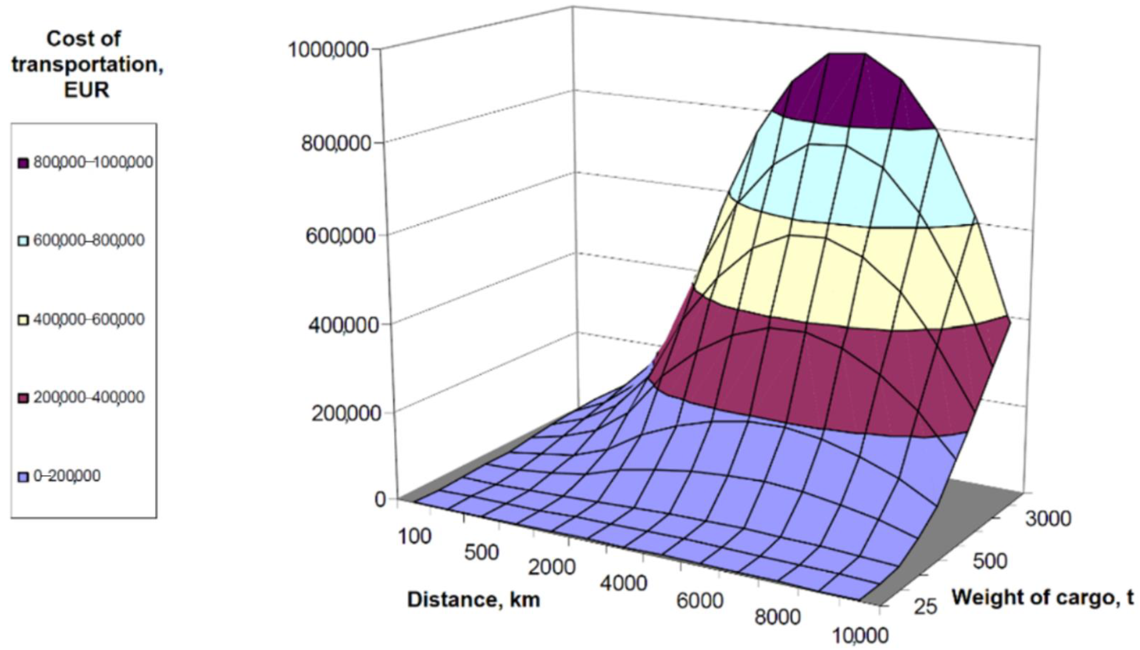
The graphical interpretation of the Formula (10) when the en-route speed of the car is 70 km/h is shown in Figure 1.
The developed formula for convenient practical use by approximate estimation of primary costs for freight vehicles. Depending on the dependence shown in the formula, we can calculate the cost of transportation by knowing the weight of the cargo and the transport distance. Fr example, if the weight of the load is 2000 t and the transport distance by car is 300 km, the cost of technological transportation is 12,642 EUR.
3.2. Calculation of the Cost of Rail Transport
Technological transport costs are estimated by determining the rate of rail transport, EUR/tkm, and are calculated according to the formula:
here: lg—distance by rail, km;
mg—the weight of the cargo that is transported by rail, t;
kg—the cost of one tkm of transport by rail, EUR/tkm.
The cost of transporting one tkm by rail depends on the speed of the railway:
here: kgv—the average cost of transport by rail, EUR/tkm;
coefficient for estimating the speed of the train.
The average cost of transport by rail depends on the distance traveled. The tariff table shows the discrete dependence of transportation rates on distance. This data is approximated by the least-squares method, and we get a gradual function. According to 2018 tariffs [53], the gradual function coefficient is 0.2047, and the degree is equal to −0.1515:
A degree of less than one means that its effect on function decreases as the transport distance increases. Minus stands for inverse proportionality—decreasing the distance, decreasing the transportation tariff. The coefficient for calculating the railway speed is calculated according to the formula:
here: ag, bg and cg—equation coefficients for rail rolling resistance [46].
Having set the coefficient values, we get:
k2 = 0.739 + 0.00325·V + 0.0814·V2
to (13) and (15) respectively inserted into Equation (12), we get:
After setting the Formula (16) to (11) and following the steps, we get:
A graphical interpretation of Formula (17) at a rail en-route speed of 40 km/h is shown in Figure 2.
Depending on the dependency shown in Equation (17), we can calculate the technological costs of transportation by knowing the weight of the load and the transport distance. For example, if the weight of the load is 500 tons and the distance of transport by rail is 200 km, then the technological transportation costs are 9173 EUR.
3.3. Calculation of Sea Transport Costs
Technological transport costs are estimated by determining the shipping price, the EUR/tkm, the relevant insurance costs and are calculated according to the formula:
here: mj—cargo weight transported by sea, t;
Cj = kj·mj;
kj—shipping costs of one tonne (t) by sea, EUR/t.
The cost of transporting one tkm by sea depends on the speed of the vessels:
here: kjv—the average cost of transport by sea, EUR/tkm;
kj = kjv·kv3
kv3—coefficient of the speed of the ship.
We calculate the average cost of shipping by sea based on the distance-based approximation of the discrete transport tariff dependence on the smallest squares method:
here: lj—distance when transporting by sea, km.
kjv = −6 × 10⁻⁶·l2j + 0.0677·lj;
The coefficient for calculating the railway speed is calculated according to the formula:
here: aj, bj, cj—equation coefficients to estimate the motion resistance of ships.
After setting the coefficient values to (21), we get:
After setting in (20) and (22), we get the Equation (23):
Kj = (−6·10−6·l2j + 0.0677·lj)·(0.8483 + 0.00373·V + 0.09338·V2);
After setting Equation (23) in Equation (18), we get:
Cj = (−6·10−6·l2j + 0.0677·lj)·(0.8483 + 0.00373·V + 0.09338·V2)·mj.
Based on 2019 data [48] function coefficients are equal to −6 × 10⁻⁶ and 0.0677, respectively. The minus sign at the square member coefficient means that the extremity of the function is the maximum. The maximum feature is at a transport distance of about 5000 km. For transportation in the European Union region up to 5000 km, we pay for the maintenance of ships, fuel, and other consumables at European prices, i.e., relatively expensive. For longer distances, maintenance can be carried out in South American or African countries, where prices are lower, leading to lower transportation rates. The ship sails between 4 and 6 thousand kilometers, fuel and maintenance costs increase, but taking advantage of cheap third-party resources does not allow such a sailing distance. This is indicated by the extreme in the appropriate graph spot. A graphical interpretation of the Formula (24) when the ship’s en route speed is 25 km/h is shown in Figure 3.
Depending on the dependency shown in Figure 3 we can calculate the technological costs of transportation by knowing the weight of the cargo and the distance of transportation. For example, in the case of sea transport, the cost of transporting 1000 t of cargo, 4000 km, will be equivalent to EUR 174,000. The same mass will cost 157,000 EUR at 8000 km. With twice the transport distance, transportation costs have not increased but have fallen. The cost reduction was due to much cheaper fuel in Asia, Africa, and South America.
3.4. Calculation of Total Technological Transportation Costs
We insert Equations (10), (17), (24) and (4) into the Equation (1). Then the total cost of transporting the goods in different modes of transport (car, rail, and sea) will be:
here: Va, Vg, Vj—route speed for the transport mode concerned, km/h;
—comparative cost by time for the relevant mode of transport, EUR/h;
—Differences between planned and actual speed , then i = a, g, j, km/h.
They evaluate unplanned vehicle downtime on the road between terminals (customs, road repair, accidents, etc.);
Ts—storage time, h, which is different at each terminal, because it depends on its technological capacity (loading device, methods), management structure and is calculated or selected individually;
—comparing costs by the time of storage in terminals, taking into account the costs of unloading and loading, EUR/h. This indicator may be determinative or variable depending on the duration of storage, type of cargo, and nomenclature of works.
As we can see from (25), in a common model for determining the cost of technology transportation, we must estimate the cost of the cargo at terminals and insurance costs. As mentioned above, these costs are quite different and depend heavily on specific stevedoring, warehousing, insurance, and specific agreements between the parties involved. Therefore, to determine the impact of purely used vehicles on the quality of the transport process, we will not evaluate the last two members of the expression (25). In the model, they will have to be assessed on a case-by-case basis.
3.5. Setting the Goal Function
For setting the goal, it used the pre-emptive priority goal programming modeling where a deviation from a higher priority level goal is considered to be infinitely more important than a deviation from a lower priority goal [50]. The quality of the freight process is determined by three key indicators: cost, time, and reliability, which also includes security. The technical safety of cargo in this model is not assessed separately, as it is quite difficult to determine it based on statistical data, and it is also different on separate routes. However, this factor is partly assessed by insurance costs. Since the factors are two, the priority queue will have two options.
Option I:
Goal function—Z = >min;
Restriction—T < Tmax.
For the first option, the goal function is to minimize costs when the transport time is limited. This is a good option when a customer wants to get a service with minimal costs and freight is not urgent. In the case of regular freight, the shipment is on the way and no matter how long it takes on the road. For example, when transporting fuel to the power plant, it is important that the power plant periodically receives a certain amount of fuel with the lowest transportation costs, and for how long the fuel will be transported and on which routes it is not important for the power plant.
Option II:
Goal function—T = >min;
Restriction—Z < Zmax.
For the second option, the purpose of the goal is to minimize the time limit for transport costs. This option is suitable when a customer wants quick delivery of goods and is willing to pay a minimum amount. For example, when delivering parts to collection workshops, they must be delivered at the right time (parts are not accumulated in modern collection workshops but delivered exactly before collection). Therefore, the delivery of parts is a priority.
3.6. An Example of Model Realization, According to Two Routes
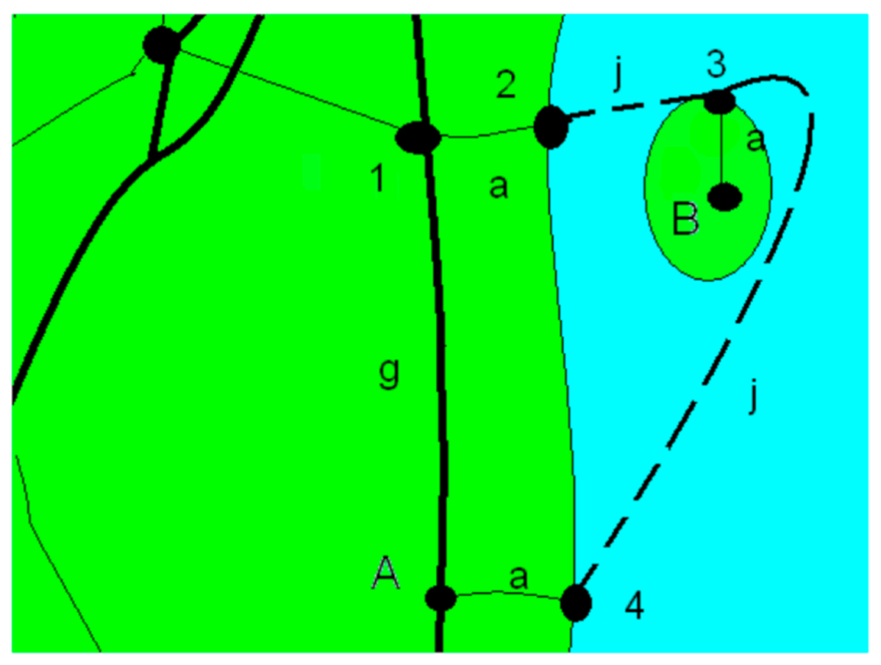
Two different theoretical routes were modeled using real transport cost data based on data collected from Lithuanian cargo companies. The first of these consists of the railway line from the starting point A to the congestion point 1, the section of the car road between the overload points 1 and 2, the section of the sea transport between the overload points 2 and 3, the car road section from the overload point 3 to the route endpoint B. The second route consists of the car road section of the road from the starting point A to the congestion point 4, the section of the route by sea transport between the congestion points 4 and 3, the car road section from the overload point 3 to the route endpoint B. Examples of the considered routes are schematically shown in Figure 4.
Figure 4 shows: A, B—start and end of routes; 1, 2, 3, 4—congestion points (terminals); a, g, j—car, rail and sea routes. Values of dimensions in the example:
expected route speeds: Car transport: Va = 70 km/h;
rail transport: Vg = 40 km/h; for sea transport: Vj = 25 km/h;
lengths of carriages are also covered: car transport, route I: la1 = 150 km;
rail transport: lg1 = 600 km; for sea transport: lj1 = 150 km;
lengths of carriages, route II: car transport: la2 = 150 km;
transporting with rail transport: lg2 = 0 km; for sea transport: lj2 = 900 km;
the weight of cargo carried is m = 2000 t.
Unforeseen vehicle downtime on the road will not be assessed yet, = 0 (we will only count the technological costs).
We assume that insurance costs are already included in the rate, so we will assume in the formula that insurance costs are zero (D = 0). However, if this is not the case, they must be evaluated. The dependence of technological transportation costs on the amount of transported cargo (according to Formula (2)) at a vehicle speed of 70 km/h is shown in Figure 5.
Taking into account the time of transportation, we assume that an entire load of cars is loaded immediately, the number of cars does not limit the volume of transportation [41,42]. If not, i.e., the cargo would be transported with a smaller number of cars, then the road and the transport time would increase accordingly.
3.7. Fluctuations in Transport Time and Cost with Vehicle Speed
If we consider the speed of one of the modes (cars) to be variable, then the solutions of the Equation (25) will take the form below (time consumption depends on the type of terminal, its stevedoring facilities, management, organization, etc.), so in each terminal, it may vary, and at the same time, the hourly price may change. In the example to be realized, we take a determinate 1-h price = 3 EUR, based on the example of the Klaipeda port terminal.
The calculation results (see Table 2) suggest that the shortest delivery time is 16.16 h on route I, with a car speed of 90 km/h, but the lowest cost will be 110,378 EUR on Route II, with an average car speed of 50 km/h.
According to the calculation results, when transporting the first route (road, rail, and sea transport) we get a graphical interpretation, which is shown in Figure 6.
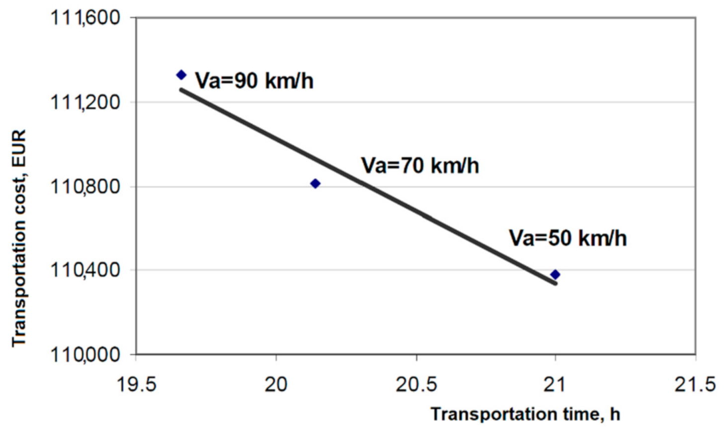
Graphical interpretation according to the second route (when transported by road and sea), changing the route speed of cars is shown in Figure 7.
We can see in the graphs that as car speeds increase, transportation time decreases and costs increase as vehicles use more fuel at higher speeds.
3.8. Transport Time Dependence on the Number of Cars Used
If the car’s load capacity is 20 t, then the transport time dependence on the number of cars used will be as follows:
here: n—the number of cars.
The graphical expression of the Formula (26) is shown in Figure 8.
The greatest impact on the number of cars have up to 50 units. Their total payload is 1000 tonnes or half of the total load. When the number of cars increases, its impact on the transport time decreases accordingly.
3.9. The General Solution of the Mathematical Model
For a set of routes according to the given methodology, we calculate the time and cost of transportation for each of them [28]. The general solution for routes I and II, where the vehicle speed is 70 km/h, is calculated based on the following data, see Table 3
When the speed of the car is 70 km/h we get a shorter time (17.14 h) on route I (road, rail and sea transport), but lower costs (110,814 EUR) on route II (road and sea transport).
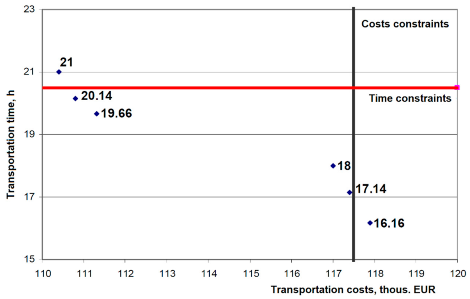
A set of points whose coordinates are transportation costs and transportation time make up the overall solution. There were two constraints on the target function setting, one on cost and one on time constraint (see Figure 9).
The overall solution was obtained by saying that the transport speed in the modes of transport is constant. In general, the most rational use of vehicles is on routes that do not go beyond time and cost constraints, but the customer can always choose the most appropriate.
3.10. Expression of the Cost of Transport Dependency, Taking into Account the Evolution of the Railway Tariff
In different European countries, rail freight rates vary, even several times. So far, we have relied on Lithuanian rail freight rates. In order to apply the calculation methodology to the transport systems of other countries, it is necessary to evaluate the development of the transportation rates of the railway, if necessary other modes [43]. A coefficient of b is used for this purpose. In the expression of the total cost of carriage, we multiply the rail freight rate by factor b. Then the expression of total costs will be as follows:
here: b—the coefficient of the change in the railway tariff.
Z = 0.02107 − (0.216 + 0.000952·Va + 0.0238 × 10⁻³·V2a)·ma·la + b·0.2047·lg0.8485·mg
0.739 + 0.00325·Vg + 0.0814 × 10⁻³·V2g) + (−6 × 10⁻⁶·l2j + 0.0677·lj)·(0.8483 + 0.00373
+0.09338 × 10⁻³·V2j)·mj + (la/∆Va)·τa + (lg/∆Vg)·τg + (lj/∆Vj) ·τj + Tsτj + ∑D
0.739 + 0.00325·Vg + 0.0814 × 10⁻³·V2g) + (−6 × 10⁻⁶·l2j + 0.0677·lj)·(0.8483 + 0.00373
+0.09338 × 10⁻³·V2j)·mj + (la/∆Va)·τa + (lg/∆Vg)·τg + (lj/∆Vj) ·τj + Tsτj + ∑D
The coefficient b shows the number of times the rail freight rate in the respective region is higher than the Lithuanian rail freight rate. The rail fare may also change for other reasons, as it may be the subject of negotiations. The general solution of the mathematical model estimating the coefficient of variation of railway tariffs b is shown in Figure 10.
In a general solution, instead of set points, we have a set of sections. This means that on each route the cost of transportation will change, with the change of rail tariffs. The railway tariff varies for a variety of reasons: different transport operators, different transport times (moments), the composition of the transport service package. Correspondingly, the total cost of transportation will vary differently, depending on the length of the sections shown in the graph.
4. Discussion
In the case of Lithuania, carriers of different types of cargo compete with each other for cargo transportation. The question arises as to how to reconcile the economic interests of all types of carriers by bringing them together for the common goal of reducing energy. The need for this research is based on a demand to promote collaboration activities of different types of cargo and to increase the effectiveness of this process, which impacts the sustainability of a particular country.
Route modeling is widely used in the public transport sector, where a passenger can reach his destination using different modes of transport. Different computer programs for routing have been developed and offered to users. In Lithuania, public transport belongs to the state and municipalities, so route modeling is an easy problem to solve. The situation is somewhat different in the field of freight transport, where many private carriers operate, transporting goods of different sizes and weights. The developed model can contribute to the development of computer programs in the field of freight transportation in Lithuania, as well as the logic of its solutions for solving transportation problems can be adapted in other countries.
One of the limitations of the model is that the ideal case is considered. The transportation process involves different private companies competing with each other for cargo that often has different purposes. In this case, the factors that reduce energy consumption are not always an advantage when choosing transportation services. The final cost of transportation also affects the country of origin of carriers who have different rates of remuneration of the drivers. Results of the research are beneficial for the optimization of the entire transport process, minimization of time or cost by selecting the most appropriate route for available roads, terminals, vehicles of a particular country, and creates a possibility to organize this process in a more effective way, creating the added value for implementation goals of Sustainable Development Agenda.
Further studies are needed to assess the factors that would help reconcile the interests of different transport companies in the field of freight transportation. The next step in the study would be to justify the economic benefits for each mode of transport individually, which could encourage the use of such a model in practice.
5. Conclusions
As a result of the research, the mathematical model was designed to optimize the entire transport process, minimizing time or cost by selecting the most appropriate route for available roads, terminals, and vehicles. The mathematical model for selecting complex vehicles in order to optimize the multimodal cargo transportation process increases energy efficiency, creates an opportunity to reduce the amount of energy required to provide products and services.
A computer experiment has been performed showing the advantages of the mathematical model created by selecting rational types and types of vehicles for cargo transportation. The model allows creating dependencies between the main indicators characterizing the transport process—the cost, the time of transport, the safety, considering the dynamics of economic and physical indicators. In the case of dependencies between the key indicators describing the transport process, it is possible to describe each of the routes in question in a specific case with two main aggregated indicators—cost Z and time T. The model enables the description of the route in a two-dimensional coordinate system, based on the constraint conditions. In the model, the linear programming problem is solved. After solving the linear programming problem, the most suitable routes and vehicles are selected according to the intended conditions. The created model could be used for rational vehicle selection by identifying the most appropriate route, minimizing transportation time and cost for the business companies.
The main advantage of the model is that the mathematical model allows to minimize transportation costs, shorten transportation time, and to select the most appropriate vehicles on a case-by-case basis from the available options depending on their environmental performance and energy saving.
There are two major limitations in this study that could be addressed in future research. First, the study focused on situation analysis in Lithuania and the investigation is based only on the data collected in this country, so this mean research could be extended by analyzing situations in others, firstly neighboring countries. However, it is possible to adapt the model for other countries, taking into consideration peculiarities. Second, the research could be extended by analyzing additional components that affect the fuel savings, as technological factors and increasing efficiency using other methods. Further on, other directions could be involved in the research.
Author Contributions
Conceptualization, J.M., V.D.; Formal analysis, O.L., J.M.; Investigation, O.L.; Methodology, O.L., J.M.; Resources, O.L., J.M., V.D.; Supervision, V.D.; Validation, O.L., J.M.; Visualization, J.M.; Writing—original draft, O.L., J.M.; Writing—review and editing, V.D. All authors have read and agreed to the published version of the manuscript.
Funding
This research received no external funding.
Institutional Review Board Statement
Not applicable.
Informed Consent Statement
Not applicable.
Data Availability Statement
Data supporting reported results can be found on http://www.degalukainos.lt/ (accessed on 18 December 2020) and https://cargo.litrail.lt/kroviniu-vezimo-tarifai (accessed on 18 December 2020).
Conflicts of Interest
The authors declare no conflict of interest.
References
- Al Majzoub, K.; Davidavičienė, V. Comparative analysis of reverse e-logistics’ solution in Asia and Europe. In Proceedings of the International Scientific Conference Contemporary Issues in Business, Management and Economics Engineering, Vilnius, Lithuania, 9–10 May 2019. [Google Scholar] [CrossRef] [Green Version]
- Burinskiene, A.; Lorenc, A.; Lerher, T. A Simulation Study for the Sustainability and Reduction of Waste in Earehouse Logistics. Int. J. Simul. Model. 2018, 17, 485–497. [Google Scholar] [CrossRef]
- Pugsley, G.; Chillet, C.; Fonseca, A. Cost-Performance-Size optimization for automotive induction machines: A fast and accurate FEM, analytical model and optimization mixed procedure. Compel Int. J. Comput. Math. Electr. Electron. Eng. 2006, 25, 297–308. [Google Scholar] [CrossRef]
- Kent, J.L.; Parker, S.R. International containership carrier selection criteria: Shippers/carriers differences. Int. J. Phys. Distrib. Logist. Manag. 1999, 29, 398–408. [Google Scholar] [CrossRef]
- Meixell, M.J.; Norbis, M. A review of the transportation mode choice and carrier selection literature. Int. J. Logist. Manag. 2008, 19, 183–211. [Google Scholar] [CrossRef]
- Nakandala, D.; Lau, H.; Zhang, J. Cost-optimization modelling for fresh food quality and transportation. Ind. Manag. Data Syst. 2016, 116, 564–583. [Google Scholar] [CrossRef]
- Lightner-Laws, C.; Agrawal, V.; Lightner, C.; Wagner, N. An evolutionary algorithm approach for the constrained multi-depot vehicle routing problem. Int. J. Intell. Comput. Cybern. 2016, 9, 2–22. [Google Scholar] [CrossRef]
- Fan, W.; Xu, H.; Xu, X. Simulation on vehicle routing problems in logistics distribution. COMPEL Int. J. Comput. Math. Electr. Electron. Eng. 2009, 28, 1516–1531. [Google Scholar] [CrossRef]
- Sandhu, M.A.; Helo, P.; Kristianto, Y. Steel supply chain management by simulation modelling. Benchmarking 2013, 20, 45–61. [Google Scholar] [CrossRef]
- Hilkevics, S.; Semakina, V. The classification and comparison of business ratios analysis methods. Insights Reg. Dev. 2019, 1, 48–57. [Google Scholar] [CrossRef] [Green Version]
- Mahdiraji, H.A.; Govindan, K.; Zavadskas, E.K.; Razavi Hajiagha, S.H. Coalition or decentralization: A game-theoretic analysis of a three-echelon supply chain network. J. Bus. Econ. Manag. 2014, 15, 460–485. [Google Scholar] [CrossRef] [Green Version]
- Chow, A.H.F.; Li, Y. Modeling and optimization of road transport facility operations. J. Facil. Manag. 2014, 12, 268–285. [Google Scholar] [CrossRef]
- Fu, L.; Liu, Q. Real-Time Optimization Model for Dynamic Scheduling of Transit Operations. Transp. Res. Rec. 2003, 1857, 48–55. [Google Scholar] [CrossRef]
- Popovič, A.; Habjan, A. Exploring the effects of information quality change in road transport operations. Ind. Manag. Data Syst. 2012, 112, 1307–1325. [Google Scholar] [CrossRef]
- Pradhan, N.; Patlolla, D.; Sawhney, R. Scheduling and route optimisation for labour cost reduction in facility custodial maintenance. J. Facil. Manag. 2017, 15, 190–206. [Google Scholar] [CrossRef]
- Karimi, B.; Ghare Hassanlu, M.; Niknamfar, A.H. An integrated production-distribution planning with a routing problem and transportation cost discount in a supply chain. Assem. Autom. 2019, 39, 783–802. [Google Scholar] [CrossRef]
- Lukinskiy, V.; Lukinskiy, V.; Merkuryev, Y. Modelling of transport operations in supply chains in obedience to ‘just-in-time’ conception. Transport 2018, 33, 1162–1172. [Google Scholar] [CrossRef] [Green Version]
- Gen, M.; Syarif, A. Hybrid genetic algorithm for multi-time period production/distribution planning. Comput. Ind. Eng. 2005, 48, 799–809. [Google Scholar] [CrossRef]
- Khalili, S.M.; Jolai, F.; Torabi, S.A. Integrated production–distribution planning in two-echelon systems: A resilience view. Int. J. Prod. Res. 2017, 55, 1040–1064. [Google Scholar] [CrossRef]
- Devapriya, P.; Ferrell, W.; Geismar, N. Integrated production and distribution scheduling with a perishable product. Eur. J. Oper. Res. 2017, 259, 906–916. [Google Scholar] [CrossRef]
- Chung, S.H.; Ma, H.L.; Chan, H.K. Maximizing recyclability and reuse of tertiary packaging in production and distribution network. Resour. Conserv. Recycl. 2018, 128, 259–266. [Google Scholar] [CrossRef]
- Vinay, V.P.; Sridharan, R. Taguchi method for parameter design in ACO algorithm for distribution-allocation in a two-stage supply chain. Int. J. Adv. Manuf. Technol. 2013, 64, 1333–1343. [Google Scholar] [CrossRef]
- Balaman, Ş.Y.; Matopoulos, A.; Wright, D.G.; Scott, J. Integrated optimization of sustainable supply chains and transportation networks for multi technology bio-based production: A decision support system based on fuzzy ε-constraint method. J. Clean. Prod. 2016, 172, 2594–2617. [Google Scholar] [CrossRef] [Green Version]
- Wang, H.F.; Chen, Y.Y. A genetic algorithm for the simultaneous delivery and pickup problems with time window. Comput. Ind. Eng. 2012, 62, 84–95. [Google Scholar] [CrossRef]
- Kuo, Y.; Wang, C.C. Optimizing the VRP by minimizing fuel consumption. Manag. Manag. Environ. Qual. An Int. J. 2011, 22, 440–450. [Google Scholar] [CrossRef]
- Li, Y.; Lim, M.K.; Tseng, M.L. A green vehicle routing model based on modified particle swarm optimization for cold chain logistics. Ind. Manag. Data Syst. 2019, 119, 473–494. [Google Scholar] [CrossRef]
- Li, L.; Yang, Y.; Tseng, M.L.; Wang, C.H.; Lim, M.K. A novel method to solve sustainable economic power loading dispatch problem. Ind. Manag. Data Syst. 2018, 118, 806–827. [Google Scholar] [CrossRef]
- Jakimavičius, M.; Burinskiene, M. Assessment of Vilnius city development scenarios based on transport system modelling and multicriteria analysis. J. Civ. Eng. Manag. 2009, 15, 361–368. [Google Scholar] [CrossRef] [Green Version]
- Shankar, R.; Choudhary, D.; Jharkharia, S. An integrated risk assessment model: A case of sustainable freight transportation systems. Transp. Res. Part D Transp. Environ. 2018, 63, 662–676. [Google Scholar] [CrossRef]
- Mesa-Arango, R.; Ukkusuri, S.V. Benefits of in-Vehicle Consolidation in Less than Truckload Freight Transportation Operations. Procedia-Soc. Behav. Sci 2013, 80, 576–590. [Google Scholar] [CrossRef] [Green Version]
- Vaquero, P.; Dias, M.F.; Madaleno, M. Portugal 2020: Improving energy efficiency of public infrastructures and the municipalities’ triple bottom line. Energy Rep. 2020, 6, 423–429. [Google Scholar] [CrossRef]
- Sarkar, A.N. Green Supply Chain Management: A Potent Tool for Sustainable Green Marketing. Asia-Pac. J. Manag. Res. Innov. 2012, 8, 491–507. [Google Scholar] [CrossRef] [Green Version]
- Ahmed, W.; Sarkar, B. Management of next-generation energy using a triple bottom line approach under a supply chain framework. Resour. Conserv. Recycl. 2019, 150, 104431. [Google Scholar] [CrossRef]
- Bataglin, M.; Ferreira, J.C.E. A modularization method based on the triple bottom line and product desirability: A case study of a hydraulic product. J. Clean. Prod. 2020, 271, 122198. [Google Scholar] [CrossRef]
- Hollos, D.; Blome, C.; Foerstl, K. Does sustainable supplier co-operation affect performance? Examining implications for the triple bottom line. Int. J. Prod. Res. 2012, 50, 2968–2986. [Google Scholar] [CrossRef]
- Burki, U.; Ersoy, P.; Dahlstrom, R. Achieving triple bottom line performance in manufacturer-customer supply chains: Evidence from an emerging economy. J. Clean. Prod. 2018, 197, 1307–1316. [Google Scholar] [CrossRef]
- Sun, Y.; Wang, P.; Lu, J.; Xu, J.; Wang, P.; Xie, S.; Li, Y.; Dai, J.; Wang, B.; Gao, M. Rail corrugation inspection by a self-contained triple-repellent electromagnetic energy harvesting system. Appl. Energy 2021, 286, 116512. [Google Scholar] [CrossRef]
- Bhuniya, S.; Pareek, S.; Sarkar, B.; Sett, B.K. A Smart Production Process for the Optimum Energy Consumption with Maintenance Policy under a Supply Chain Management. Processes 2021, 9, 19. [Google Scholar] [CrossRef]
- Sabaitytė, J.; Davidavičienė, V.; Van Kleef, G.F. The Peculiarities of Low-Cost Carrier Development in Europe. Energies 2020, 13, 639. [Google Scholar] [CrossRef] [Green Version]
- AL Majzoub, M.; Davidavičienė, V.; Meidutė-Kavaliauskienė, I. Measuring the impact of factors affecting reverse e-logistics‘ performance in the electronic industry in Lebanon and Syria. Indep. J. Manag. Prod. 2020, 11. [Google Scholar] [CrossRef]
- Batkovskiy, A.M.; Kalachikhin, P.A.; Semenova, E.G.; Telnov, Y.F.; Fomina, A.V.; Balashov, V.M. Conficuration of enterprise networks. Entrep. Sustain. Issues 2018, 6, 311–328. [Google Scholar] [CrossRef]
- Mishenin, Y.; Koblianska, I.; Medvid, V.; Maistrenko, Y. Sustainable regional development policy formation: Role of industrial ecology and logistics. Entrep. Sustain. Issues 2018, 6, 329–341. [Google Scholar] [CrossRef]
- Otter, C.; Watzl, C.; Schwarz, D.; Priess, P. Towards sustainable logistics: Study of alternative delivery facets. Entrep. Sustain. Issues Entrep. Sustain. Cent. 2017, 4, 460–476. [Google Scholar] [CrossRef] [Green Version]
- Litman, T. Developing indicators for comprehensive and sustainable transport planning. Transp. Res. Record. 2007, 2017, 10–15. [Google Scholar] [CrossRef] [Green Version]
- Guo, Y.; Lim, A.; Rodrigues, B.; Zhu, Y. Carrier assignment models in transportation procurement. J. Oper. Res. Soc. 2006, 57, 1472–1481. [Google Scholar] [CrossRef] [Green Version]
- Bogdevičius, M.; Junevičius, R.; Vansauskas, V. Transporto Priemonių Dinamika; Technika: Vilnius, Lithuania, 2012; Available online: http://dspace.vgtu.lt/jspui/bitstream/1/1436/1/1381-S_Bogdevicius_Transporto_WEB.pdf (accessed on 20 December 2020).
- Gerasimov, B.N.; Vasyaycheva, V.A.; Gerasimov, K.B. Identification of the factors of competitiveness of industrial company based on the module approach. Entrep. Sustain. Issues 2018, 6, 677–691. [Google Scholar] [CrossRef]
- Korauš, A.; Mazák, M.; Dobrovič, J. Quantitative analysis of the competitiveness of Benelux countries. Entrep. Sustain. Issues 2018, 5, 1069–1083. [Google Scholar] [CrossRef]
- Liao, Z.; Rittscher, J. Integration of supplier selection, procurement lot sizing and carrier selection under dynamic demand conditions. Int. J. Prod. Econ. 2007, 107, 502–510. [Google Scholar] [CrossRef]
- Tizroo, A.; Esmaeili, A.; Khaksar, E.; Šaparauskas, J.; Mozaffari, M.M. Proposing an agile strategy for a steel industry supply chain through the integration of balance scorecard and Interpretive Structural Modeling. J. Bus. Econ. Manag. 2017, 18, 288–308. [Google Scholar] [CrossRef] [Green Version]
- Aköz, O.; Petrovic, D. A fuzzy goal programming method with imprecise goal hierarchy. Eur. J. Oper. Res. 2007, 181, 1427–1433. [Google Scholar] [CrossRef]
- Degalų Kainos. 2020. Available online: http://www.degalukainos.lt/ (accessed on 18 December 2020).
- JSC Lithuanian Railways. Available online: https://cargo.litrail.lt/kroviniu-vezimo-tarifai (accessed on 18 December 2020).
Figure 1.
Dependence of car transport costs.

Figure 2.
Dependence of rail transport costs.

Figure 3.
Dependence of sea transport costs.

Figure 4.
Scheme of freight route.

Figure 5.
Dependence of technological transportation costs on the amount of transported cargo.

Figure 6.
Technological transportation costs according to the first route.

Figure 7.
Technological transportation costs according to the first route.

Figure 8.
Transport time dependent on the number of cars used.

Figure 9.
Graphical expression of overall the solution.

Figure 10.
General solution of a mathematical model estimating the coefficient of variation of railway tariffs b.
Figure 10.
General solution of a mathematical model estimating the coefficient of variation of railway tariffs b.


Table 1.
Contribution to the subject of the previous authors.
| Factors | Components | Authors |
|---|---|---|
| 1. Efficient organization of freight transport | Production planning | [4,14,16,19,21,38,41] |
| Distribution planning | [4,8,16,19,21,22,31] | |
| Equipment availability factors | [4,14] | |
| Rate change | [4,6,10,29,31,38] | |
| Financial management | [4,10,11,31] | |
| Services quality | [1,4,8,11,13,16,23,24,30,41,42,43] | |
| Transport operation | [4,14,17,20,23,25,44,45,46], this paper | |
| Market value | [10,11,32,33,34,42,43,47,48] | |
| Triple bottom line | [31,32,33,34,35,36,37] | |
| Delivery time | [9,14,17,29,40], this paper | |
| 2. Transportation mode choice | Mode choice | [3,5,11,14,23,44], this paper |
| Carrier selection | [4,5,30,35,39,49], this paper | |
| Environmental use concerns | [1,5,10,26,35,44,47], this paper | |
| Energy use concerns | [5,6,23,26,31,33,37,38,41,44], this paper | |
| Vehicle routing | [7,8,12,13,14,15,24,26,29,30,44], this paper | |
| Supply chain networking | [5,9,11,14,16,17,23,26,29,32,33,38,48,50] | |
| Logistics operation | [8,14,17,18,21,24,29,40,41,42,49], this paper | |
| Fuel consumption | [12,23,25,28], this paper | |
| Information quality | [9,13,14,15,29,40,41,47] | |
| Technological development | [8,10,14,26,32,40], this paper | |
| Supply chain simulation | [9,11,36] | |
| An appropriate time buffer | [8,9,13,15,23,29,30,42,49,51] | |
| Decentralization case | [11] | |
| 3. Optimal routes choose | Route planning | [2,5,15,42], this paper |
| Transportation capacity | [5,9,12,23,24,30,45] | |
| Economies of scale and scope | [5,23,30,34,36,45,48], this paper | |
| Minimization the total distance of all the vehicle | [9,12,28,30], this paper | |
| Minimize the total number of vehicle | [12,28,30], this paper | |
| Service the customers as punctually as possible | [1,8,9,42] | |
| Sensitivity to demand | [7,9,11,12,16,18,26,27,30,41] | |
| Just-in-time | [9,17] | |
| Cost reduction | [3,6,9,11,15,16,24,25,27,29,35,39,41,43], this paper | |
| 4. The multifunctional problem of optimization/Performance of existing transport facilities | Multi-objective optimization problem | [6,7,8,16,19,26,27,32,33,49,51], this paper |
| Non-dominated sorting genetic algirithm II (NSGA-II) | [8] | |
| Case study | [5,6,9,11,12,14,15,25,26], this paper | |
| System dynamic approach | [2,10,19,41,49], this paper | |
| Simulation model | [2,3,5,8,9,17] | |
| Finite-element-method (FEM) | [3,12] | |
| Math model | [10,11,12,13,16,18,24,43,48], this paper | |
| Linear model | [2,6,12,19,20,24,30,32,46,47,48,51] | |
| Cell transmission model | [12,20,46] | |
| Real-time optimization model | [3,13] | |
| Conceptual model | [5,9,29,35,41,43,50] | |
| Non-linear model | [3,7,11,13,16,27,38,46] | |
| Genetic algorithm | [5,6,7,8,16,18,24,26,27,34,49] |
Table 2.
Estimation of routes I–II, cost and delivery time.
| Route I: There are three variants of expected speed for car transport, when: Va = 50 km/h; 70 km/h; 90 km/h. | ||
| Va = 50 km/h | tg1 = 600/50 = 12 h; | T1= tg1+ ta1+ tj1 = 18 h, |
| ta1 = 150/50 = 3 h; | Z1 = 115,169 + 18*100 = 116,969 EUR | |
| tj1 = 150/50 = 3 h. | ||
| Va = 70 km/h | tg3 = 600/50 = 12 h; | T3= tg3+ ta3+ tj3 = 17.14 h, |
| ta3 = 150/70 = 2.14 h; | Z3 = 115,650 + 17.14 × 100 = 117,364 EUR | |
| tj3 = 150/50 = 3 h. | ||
| Va = 90 km/h | tg5 = 600/50 = 12 h; | T5= tg5+ ta5+ tj5 = 16.16 h, |
| ta5 = 150/90 = 1.66 h; | Z5 = 115,169 + 16.16 × 100 = 117,868 EUR | |
| tj5 = 150/50 = 3 h. | ||
| Route II: There are three variants of expected speed for car transport, when: Va = 50 km/h; 70 km/h; 90 km/h. | ||
| Va = 50 km/h | tg2 = 0 h; | T2= tg2+ ta2+ tj2 = 21 h, |
| ta2 = 150/50 = 3 h; | Z2 = 108,278 + 21 × 100 = 110,378 EUR | |
| tj2 = 900/50 = 18 h. | ||
| Va = 70 km/h | tg4 = 0 h; | T4= tg4+ ta4+ tj4 = 20.14 h, |
| ta4 = 150/70 = 2.14 h; | Z4 = 108,800 + 20.14 × 100 = 110,814 EUR | |
| tj4 = 900/50 = 18 h | ||
| Va = 90 km/h | tg6 = 0 h; | T6= tg6+ ta6+ tj6 = 19.16 h, |
| ta6 = 150/90 = 1.66 h; | Z6 = 109,361 + 19.16 × 100 = 111,327 EUR | |
| tj6 = 900/50 = 18 h. | ||
| Calculation results: | ||
| when Va = 50 km/h. | then T1 = 18 h; | Z1 = 116,969 EUR; |
| T2 = 21 h; | Z2 = 110,378 EUR. | |
| when Va = 70 km/h. | then T3 = 17.14 h; | Z3 = 117,364 EUR; |
| T4 = 20.14 h; | Z4 = 110,814 EUR. | |
| when Va = 90 km/h. | then T5 = 16.16 h; | Z5 = 117,868 EUR; |
| T6 = 19.66 h; | Z6 = 111,327 EUR. | |
Table 3.
Estimation of routes I–III, general solution.
| Route I: | ||
| Va = 70 km/h | tg3 = 600/50 = 12 h; | T3= tg3+ ta3+ tj3 = 17.14 h, |
| ta3 = 150/70 = 2.14 h; | Z3 = 115,650 + 17.14 × 100 = 117,364 EUR | |
| tj3 = 150/50 = 3 h. | ||
| Route II: | ||
| Va = 70 km/h | tg4 = 0 h; | T4= tg4+ ta4+ tj4 = 20.14 h, |
| ta4 = 150/70 = 2.14 h; | Z4 = 108,800 + 20.14 × 100 = 110,814 EUR | |
| tj4 = 900/50 = 18 h | ||
| Calculation results: | ||
| T3 = 17.14 h | Z3 = 117,364 EUR | |
| T4 = 20.14 h | Z4 = 110,814 EUR |
Publisher’s Note: MDPI stays neutral with regard to jurisdictional claims in published maps and institutional affiliations. |
© 2021 by the authors. Licensee MDPI, Basel, Switzerland. This article is an open access article distributed under the terms and conditions of the Creative Commons Attribution (CC BY) license (https://creativecommons.org/licenses/by/4.0/).
Share and Cite
MDPI and ACS Style
Lingaitienė, O.; Merkevičius, J.; Davidavičienė, V. The Model of Vehicle and Route Selection for Energy Saving. Sustainability 2021, 13, 4528. https://doi.org/10.3390/su13084528
AMA Style
Lingaitienė O, Merkevičius J, Davidavičienė V. The Model of Vehicle and Route Selection for Energy Saving. Sustainability. 2021; 13(8):4528. https://doi.org/10.3390/su13084528
Chicago/Turabian StyleLingaitienė, Olga, Juozas Merkevičius, and Vida Davidavičienė. 2021. "The Model of Vehicle and Route Selection for Energy Saving" Sustainability 13, no. 8: 4528. https://doi.org/10.3390/su13084528
Note that from the first issue of 2016, this journal uses article numbers instead of page numbers. See further details here.