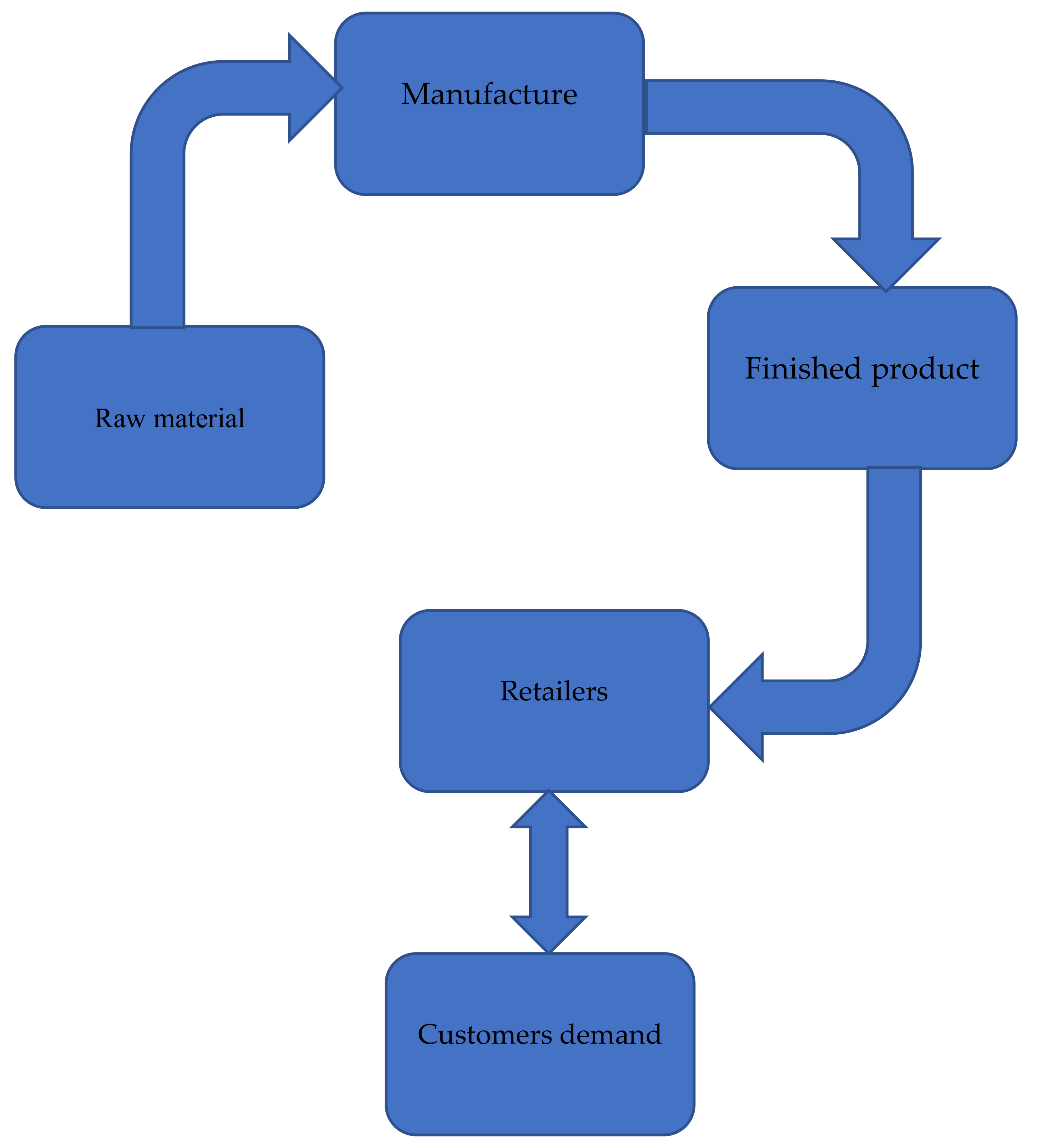
An Investigation of a Supply Chain Model for Co-Ordination of Finished Products and Raw Materials in a Production System under Different Situations

Abstract

In the production system, the production of a perfect item is essential for existing competitive market situations. To produce a perfect finished product, the quality of a raw material is a crucial issue of a production system. This paper has examined this issue with an insightful production-inventory model of the manufacturer of a deteriorating item selling goods to multiple markets with different selling seasons. We have provided an answer strategy to track down the optimal production plan for raw materials and the ideal creation plan for completed items. Transportation cost was incorporated for transporting the raw material. Marketing of the finished product is another crucial factor for selling products and earning revenues. The main objective of the present study is to adopt a production model in inventory for inferring request capacities for multi-item, multi-outlet circumstances. As of late, much accentuation has been given to the consideration of the control and support of creation inventories of disintegrating things. The demand rate is persistent and holding cost is a direct function of time. This paper has followed an analytical approach to diminish the entire inventory cost. Finally, a sensitivity analysis was performed to study the effect of changes of different parameters of the model on the optimal policy. Moreover, in order to approve the determined models, we have clarified mathematical models and examined affectability.

1. Introduction

The introductory section consists of three parts. The first part consists of the motivation of research work, whereas the second part is a reported literature review. In the third and final part, the research gap and contribution are described.

1.1. Motivation (General Problem Description)

Inventory is the most fascinating and profoundly investigated subject of production and activity of executives. Inventory, being a fundamental piece of our lives since the start of development, is found all around as family inventory, social inventory and business inventory. Inventory bears the cost of adaptability; however, it begins at an expense. Inventory might be viewed as the capacity of a thing that would be utilized to satisfy the future requests of that thing. Along these lines, inventory of the board requires a logical inventory model. The timeliest consistent inventory and the load-up approach originate from the second decade of the earlier century. It very well may be concurred that the peak time for research on inventory was from the 1950s to the 2000s. It was stretched theoretically and represented the inventory problem mathematically being articulated. A variety of interests regarding time and cost are some of the significant factors in any inventory framework. Few investigations have reported circumstances where request changes with time and cost independently. A couple of analysts have thought about the collective impact of cost and time on ideal arrangements.

Many studies have been conducted in the inventory board field in order to develop financial (economic production quality—EPQ) inventory models. Each assembly association needs to convey the best item to clients since they worry about buying things in the present cut-throat world. This prompts producers to contribute more to the progress of the assembling cycle. It is undeniably true that one cannot disregard the impact of the deterioration of items. Subsequently, to lessen the deterioration rate, the producer can utilize some extraordinary advancements such as refrigeration of things. This innovation is known as preservation innovation. Many studies finished by considering the above-mentioned innovation; however, considering a production inventory model for weakening things with multiple markets demands diverse creation rates and preservation innovation together. In a large portion of the news articles, it is shown that the production rate all through the period is the same, which is not exactly sensible. The holding cost is not always constant. It depends on the market situation. Thus, we took time-dependent linear holding costs to manage market competition criteria. This inspired us to consider such an assembling framework with distinctive creation rates over the cycle time frame. Regarding this issue, this paper considers numerous market demand diverse creation levels. It is accepted that the creation rate is at a lower rate at first and it increases dynamically over the creation cycle. This is simply to decrease the holding cost by sidestepping the higher stock amount at first. Moreover, this creation inventory model considers these deficiencies, which are all placed in a rain check.

1.2. Literature Review

The essential exploration regions applicable to this paper are underlined here. In this subsection, we examine about the essential exploration conducted in the space of stock models given as (1) deterioration with preservation technique, (2) time-dependent holding cost, (3) multiple market demand, (4) shortage facilities, (5) and supply chain facilities.

Deterioration is observed continuously in everything. It may be low or high for different items. Inventory models for breaking down things are varied, the more significant part of which consider a consistent deterioration rate over the long-haul of things practically speaking, similar to unstable fluids, horticultural items, etc. The impact of decaying is huge in numerous inventory frameworks. Food stuffs, prescriptions and radioactive ingredients are models in which significant deterioration can occur during the reasonable stockpiling time of the units. It seems reasonable to expect the holding cost to be a period of subordinate capacity. The inventory plot for decaying things has been an article of amendment for quite some time. In any case, barely any studies have examined the impact of placing resources into diminishing the pace of item deterioration. Mishra and Sahab [1] built up the perfect principal creation part size—perfect in a consistent and variable pace of deterioration. The production models expect that all things are fabricated for top caliber and that bad things are created. It is the case, however, that bad things show up in many assembling frameworks; specialists create production models for inadequate creation frameworks. Thus, in creation frameworks, bad things are of two sorts: rejected things and rewardable things. Khara et al. [2] investigated an imperfect production system that produced perfect items and defective produce. Generally, factory-made products are scrutinized with a 100% transmission procedure and defective products detach from all the produced items. All perfect products retailed and defective products are either repaired or sold at a reduced price. Benkherouf et al. [3] analyzed the impacts of assembling out-of-order things on a production model. The authors guessed that a steady rate of revamps damaged things after finishing the normal creation cycle. Manna et al. [4] presented a ton estimating tricky for an imperfect exchange framework with ad subordinate interest and mechanical rate reliant upon the flawed rate. As of late, scientists and researchers have examined the inventory issues with different approaches such as Bera and Jana [5], Mahata [6] Nobil et al. [7] and Dizbin et al. [8]. In this flawed deteriorating manufacturing system, the machine produces a defective product and imperiled superiority deterioration. Some authors considered non-instantaneous deterioration. For instance, Maihami and Kamalabadi [9] discussed that a control issue that limits the regular expense of the framework in the consistent state by controlling when creating an accessible part. The optimal control strategy is the state-subordinate edge strategy. For non-instantaneous decaying things, cost and time-subordinate interest have been considered by Ghoreishi et al. [10]. Yang et al. [11] dealt with determining the optimal replenishment policy for constant deterioration rate with a stock-dependent request in which the deadly stage of zero-ending inventory is relaxed and shortages are permitted. Banerjee and Agrawal [12] obtained an optimal omitting policy that was a concession offer after the inauguration of deterioration. In practice, the deterioration rate of an item is controlled by various preservation techniques and reduced various exertions such as procedural fluctuations and specialized equipment purchase, etc. The consideration of preservation innovation/technology (PT) is imperative because of preserving the product for long time and how PT can essentially lessen the decaying amount by decreasing monetary misfortunes, increasing client support and incrementing marketing intensity. The effect of preservation technology investment was studied by a few researchers Hsu et al. [13], He and Huang [14], Dye [15], Mishra et al. [16] analyzed. Sean et al. [17] analyzed a production model under an uncertain preservation technique method. Bardhan et al. [18] mentioned that the highest score replenishment protection and preservation era investment for a non-right is now deteriorating object with the inventory-hooked-up call. Mashud et al. [19] invested in non-momentary crumbling, settlements ahead of time and incomplete rain check systems. The outcomes and affectability examination show the positive effects of controllable fossil fuel by-products and decay on the absolute stock model benefit. Taleizadeh [20] described an integrated flawed industrial system that deals under protective conservation and fractional back ordering for a defective item.

As of late, a significant pattern has updated a creation framework by running or making variable creation rate inside some static stretch to keep up the ideal level. In a market situation, holding costs cannot be constant. It changes as a linear. An inventory system is efficient when the holding cost depends on time while it is interrelated with the length of holding of product and pace of creation. This exploration hole is satisfactory as studied by Sarkar and Lee [21]. They demonstrated that for packaging strategy of cost of holding and the creation pace of the two makers that produce correlative items, assume some significant parts inside the inventory network. Alfares and Ghaithan [22] demonstrated that time depending on holding cost assumes a significant part and Sarkar et al. [23] created the impact of variable creation rate, which is near the impact of time-dependent holding cost is the fundamental inventory model. Hence, the prompt examination hole emerges: the component of the store network model under holding cost depends on time and request-dependent creation rate for both the makers and those who might want to deliver essential, integral items. Pervin et al. [24] explained that a time-dependent interest approach is acquainted with showing the appropriateness of our proposed model fully informed regarding admiration to time. The principal motivation behind the paper is to explore the ideal retailer’s renewal choices for decaying things, including time-dependent interest for exhibiting more reasonable conditions inside financial request amount structures. Leopoldo [25] analyzed how the holding cost can play an indivisible role in production. For more explicitly, it increases with time since an extensive stretch of capacity requires more costly stockroom offices. This examination presents an inventory model with deficiencies for a solitary item where the interest rate depends on the selling cost and time as indicated by a force design. Palanival and Sugunya [26] say the article manages a full expanding benefit for inventory ideal arranged amount and halfway multiplying with the holding cost contingent upon the capacity period. The pace of market request is accepted to vacillate as a capacity, given stock and selling cost. Mishra [27] built up an inventory model of immediate falling apart things with a sensible deterioration rate for time-subordinate interest and holding cost.

Similarly, a few scholars’ studies are on multiple-market and multiple variate’s demands: Nasr et al. [28] has explained an economic production quantity (EPQ) classical with deteriorating raw material and investigated the impact of the deterioration of the production progression. The EPQ corrupt case with no decline presented where the raw material is methodical for multiple production cycles. Bhunia and Shaikh [29] built an endeavor to make two inventory models for uniform weakening things with variable interest subordinate rates on the selling cost and recurrence of commercial things. Duari and Chakraborti [30] analyzed a production inventory model, whereas demand depends on the selling price and multiple market demands. They measured deterioration in quality amount to begin from the age of appearance of the things in stock. Nobil [31] and Al et al. [32] inferred a multi-item production model with discrete conveyance arranges and compelled spaces. They improved their model under a hereditary calculation. They considered a creation framework that manufactures multi-items that are shipped off a purchaser by bunches. Uthayakumar and Tharani [33] explained remanufacturing cycle might forestall removal costs and decrease ecological quandaries. A financial creation amount model has been depicted for weakening things with modifying and different cremation arrangements to beat this issue. In the end, a portion of the similar works is introduced in

Table 1. Recent and related work related to inventory literature.

Authors	Deterioration (Constraints)	Demand Function	Holding Cost	Preservation	Shortage
He et al. [34]	Constant	Constant	Constant	No	No
Singh et al. [35]	Weibull distribution	Time-dependent	Constant	No	Allowed
Sajadifar and Hashempour [36]	Constant	Constant	Constant	No	Allowed
Malik and Sharma [37]	Constant	Linear	Constant	No	Allowed
He and Wang [38]	Constant	Disruption	Constant	No	No
Karimi and Sadjadi [39]	Discrete	Time-dependent	Constant	No	Allowed
Singhal and Singh [40]	Weibull distribution		Linear increasing	No	Not Allowed
Chakraborty et al. [41]	Constant overtime	Stock dependent	Constant	No	Allowed
Pal et al. [42]	Constant	Time-dependent	Constant	No	Not Allowed
Khurana [43]	Weibull distribution	DeterministicLinear	Constant	Yes	Not Allowed
Tiwari et al. [44]	Non-instantaneous	Stock dependent	Constant	---------	Allowed
This Paper	Controllable	Constant	Linear	Yes	Allowed

.

This paper presents a multiple-market inventory model for falling apart things with time-shifting holding costs and a reliable, controllable deterioration rate for everything. In this examination, deficiencies with fractional accumulating are permitted. However, there is a cut-off limit of a transporter and we are not permitted to arrange an endless number of items. Since there is no vehicle with a limitless limit, in fact, this is a reasonable presumption that makes the created model more logical. The time skyline is limited and constant; however, the choice factors for the beginning season of deficiency are discrete.

The word shortage implies a state or circumstance where the required things cannot acquire inadequate sums or miss. To clarify the circumstance more plainly, we can guess that an organization delivers some actual merchandise whose request increases out of nowhere or quickly and the organization cannot supply the item because of some unavoidable conditions. As a result, shortages happen for this specific item to the clients. Shortages are vital for some models, particularly when a delay is made in instalment. During a shortage, the organization offers a delay in instalment. It can acquire orders from the clients. Along these lines, shortages can appreciate an incredible benefit for offering delay in instalment. In inventory models with shortages, the general supposition is that unfulfilled interest is either lost or accumulated. Another significant contemplation in inventory issues is the consideration of deficiency which implies that the creation framework faces a lack which is delay purchased or lost a deal, Jauhari and Pujawan [45] Thinakaran et al. [46] Taleizadeh et al. [47] addressed inventory problems with a shortage. They find the optimum level of shortage with deference to maximizing the system’s profits. Singh [48] studied a production model with subordinate request creation and a consistent decaying rate for the supposition of fractional multiplying. Gothi and Parmar [49] proposed one logarithmic arrangement strategy without subordinates to find the ideal EPQ inventory model with deficiency. Palanivel and Uthayakumar [50] introduced a monetary creation amount (EPQ) prototypical under probabilistic corrosion rate, variable creation and incomplete multiplying under selling rate. Inventory stockpiling is beneficial. This is also valuable from an economic point of view, for structure cost is significantly decreased by permitting shortages. Cardenas–Barron [51] introduced a total audit of more than a few advancing strategies in the inventory hypothesis. In exploring their model, he established the ideal answer for inventory issues with two sorts of delay purchase costs, straight and fixed and mathematical strategy. Then, Taleizadeh et al. [52] established a constrained combined defective manufacturing–inventory system with protective conservation and partial backordering. Inventory is an extent or store of stock held in stock and established a solitary mechanism system for multi-items defectives with unfinished backordering. The effects of partial backlogging and shortage with time-dependent demand have been explained by many researchers, such as Prasad and Mukherjee [53], De and Sana [54], San-Jos et al. [55], Sarkar [56]. Chaudhary et al. [57] built up an inventory model for weakening things where time-differing conveying cost, stock ward request and deficiency are allowed to be adequately multiplied. We and Lee [58] devolved an EOQ inventory model for Weibull distributed deterioration to take shortages and time-varying demand.

Managers of any supply chain continuously improve their performance by reducing lead time and its variance. A supply chain for the multi-purchase and the single-seller with FPR and sub-par nature of items was created by Sarkar et al. [59]. A supply chain model under the idea of LTR with FPR was introduced by Dey et al. [60], where they decrease the lead time by diminishing arrangement time and conveyance time. The idea of arrangement cost decrease and cycle quality improvement was consolidated in their model; however, they fostered their consistent interest model. Sett et al. [61] present review centers around a single-vendor, single-purchaser supply chain model for a single kind of item with updated administration given to the purchaser by the vendor. Vendors frequently increase their benefit by providing a lower quality of a specific item. Dey et al. [62] discussed that controllable lead time and fluctuation are fundamental issues for the executives’ keen supply chain. This review worries about variable lead time and difference under controllable creation rate and publicizes subordinate interest. This paper investigates and evaluates these advantages of such lead time decrease for generally utilized parcel size amount, creation rate, security factor, reorder point, commercial expense and merchant’s arrangement cost.

For the research gap, He et al. [34] discussed the first multiple market demand model. They discussed that developing the variation in decaying products at altered markets provides an exclusive chance to increase a deteriorating items’ manufacturer’s productivity. Sajadifar and Hashempour [36] have extended this research work using this model with shortage facilities. After that, some research work on multiple markets and multi-variate with constant deterioration rate and holding cost are analyzed in Table 1. In inventory model, it is expected that the holding cost is known and constant. However, holding costs may not generally be constant. In most cases, inventory is genuinely saved in stockrooms to fulfil the customer’s needs or for future use. Accordingly, factor holding cost draws in the more significant part of the connected analyst’s consideration because keeping up inventory is incredibly essential. Holding cost is likewise very high and reliant upon short-lived things, e.g., organic products, vegetables, medication or unpredictable fluids. Henceforth, to be fully informed regarding the current market circumstance, variable holding cost is most significant.

Nevertheless, no one uses time-dependent holding cost with controllable deterioration rate. So, we take controllable deterioration rate with time-dependent holding cost. The real inspiration of the paper is as per the following. Among the different requests in EOQ models, the time-subordinate holding cost approach is entirely reasonable to address an ideal practical circumstance. We consider non-immediate breaking down things and shortages to show the actual condition to address more practical conditions. The primary issue is to limit the high all-out cost by improving the cycle length. We propose a monetary request amount inventory model to get the ideal credit time frame and process duration from the retailer’s viewpoint when the deterioration rate follows a controllable crumbling that gives a more extensive application scope. In addition, a graphical representation of the problem definition is provided below in Figure 1.

1.3. Research Gap and Contribution

He et al. [34] analyzed various business sectors throughout the planet to allow the maker to sell the items in various periods and topographical areas and accomplish higher benefits. Singh et al. [35] explained that an inventory model is introduced to decide the optimal renewal cycle for two-stockroom inventory issues under swelling, changing pace of deterioration and incomplete putting in a rain check with stock and time subordinate demand. Sajadifar and Hashempour [36] described the production inventory model with partial backlogging. Malik and Mishra [37] discussed an EOQ model for falling apart with multi-variate demand under the supplier’s exchange credit office under the two particular cases. Holding cost is time-dependent and unsatisfied demands are backlogged. He and Wing [38] explained the production model with disruption demand. Karimi and Sadjadi [39] consider multi-item models with a limit or spending imperatives—a direct result of the nonlinear conduct of these models and the intricacy of the nonlinear improvement strategy. Singhal and Singh [40] investigated an incorporated transient things inventory renewal model for rotting things with multiple market demands under volume adaptability. Adaptability is an alluring property of creation frameworks regularly introduced as a panacea to various reasonable issues. Chakraborty et al. [41] examined a multi-thing inventory model for non-momentary falling apart under expansion in an unpleasant climate with multiple distribution centre offices. One is a claimed stockroom and the others are leased distribution centers with restricted capacity limits. Pal et al. [42] discussed three-layer multi-item manufacture–inventory model for multiple dealers and vendors. Khurana [43] investigated the impacts of crumbling in both the stockrooms and have considered a steady pace of weakening. In any case, we have taken a straight-time subordinate disintegration rate and Weibull dissemination type crumbling rate in raw materials. Tiwari et al. [44] discussed a two-distribution centre inventory model for non-momentary decaying things with fractional multiplying and stock-subordinate demand under inflationary conditions. Deficiencies are permitted. The multiplying rate is variable and relies on the hanging, tight an ideal opportunity for the next renewal. In this paper, the following factors are incorporated to investigate the present model:

(i).

Controllable deterioration, i.e., preservation technology, is introduced;

(ii).

Time-varying holding cost is incorporated;

(iii).

Shortages are allowed.

The rest of the paper is systematic. Section 2 delivers the aims of study, the notation/ symbolizations and the suppositions to frame the proposed inventory model. Section 3 discusses the mathematical formulation and cost calculation of the manufacture of finished products inventory system with the shortage. Section 4 derives theoretical formulation of cost calculation of raw material and manufacture finished products. Section 5 discusses the result with the help of a numerical guide to illustrate the planned model. Section 6 presents the sensitivity analysis of the essential parameter and graphical representation. Section 7 shows the managerial implication of the study. Section 8, the final section, concludes the overall findings with suggestions, limitations and guidance for future research work.

2. Nomenclature and Assumptions

In this section, we define the preliminary aspects necessary to develop the proposed model and formulate the related optimization problem. In particular, this section introduces the following symbolizations and assumptions that are used.

2.1. Symbolizations/Nomenclature

The main notation adopted in this paper is listed below.

Parameters

(a)

$c_p$= component production cost of the decaying product. [units]

(b)

$p$ = rate of production. [$/units)]

(c)

${\theta }_2$= persistent deterioration amount of finished products. [quantity unit/unit time]

(d)

${\theta }_p$= resultant deterioration rate ${\theta }_p={\theta }_2{e}^{-\alpha \xi }$.

(e)

Reduced deterioration rate of the finished product where $mi\left(\xi \right)=\theta i\left(1-e^{-\alpha \xi }\right)$

(f)

$k_0$= setup cost. [setup/$]

(g)

$d_i$= demand rate of market from one to three $i=1,2,3$. [$/units/quantity unit]

(h)

$s_i$= selling season of market from one to three $i=1,2,3$. [$/units]

(i)

$c_b$= backlogging cost per unit. [$/unit]

(j)

$c_{fc}$= purchase cost of finished products. [$/unit]

(k)

$T{S}_p$= the purchase cost of finished products. [$/quantity unit/unit time]

(l)

$T{B}_p$= the backlogging cost of finished products. [unit time]

(m)

$T{C}_p$= the total cost of finished products goods [$/units]

(n)

$TC$= total cost [$/order]

(o)

$I_i(t)$= inventory level in the $i^{th}$ interval $i=1,2,3\dots u,u+1,\dots T$. [units]

The restrictions of raw materials cost by the constructer are as follow:

(a)

$s_r$ = component price of ordering cost. [($/order)]

(b)

$c_r$ = component price of raw materials. [unit]

(c)

$h_r$ = holding price of raw material per unit time for manufacturing. [unit/unit time]

(d)

${\theta }_1$ = constant deterioration rate of raw materials. [unit time]

(e)

${\theta }_r$ = resultant deterioration rate ${\theta }_r={\theta }_1{e}^{-\alpha \xi }$ of raw materials. [quantity unit/unit]

(f)

$f$ = procedure unit of raw constituents per finished product. [$/order]

(g)

$c_p$= purchased cost per unit finished product. [quantity unit/unit time]

(h)

$c_t$= transportation cost per lot [$/shipment]

(i)

$T{C}_r$= total cost of raw materials. [$/unit]

Dependent Variable

(a)

$T_1$ = Optimal time. [time unit]

Decision Variable

(b)

$n_r$ = Number of raw materials deliveries from the supplier to manufacture. [Positive integer]

(c)

$q_r$ = Lot-size per delivery from supplier to manufacture. [$/unit]

(d)

$\xi$ = Preservation technology (PT) charges for dropping deterioration rate in instruction to preserve the product. [in $].

2.2. Assumptions

The main assumptions considered to develop the model are given below:

(1)

The rate of production is deterministic and constant [2,34,36].

(2)

The inventory system studies a single item, a single manufacturer and multiple markets over a known [34,36].

(3)

The rate of production $p$ is more significant than any selling price rate of demand.

(4)

The finite planning horizon is considered [1,34].

(5)

Deterioration rates of the materials and finished products are deterministic and controllable [1].

(6)

Total cost $TC=T{C}_p+T{C}_r$ where $T{C}_p$ the total cost of finished products goods and $T{C}_r$ is the total cost of raw materials [34,36].

(7)

Primetime is null or negligible [1,10,34,53].

(8)

The demand rate is constant and identified [34,36].

(9)

There is no repair or replacement of deteriorated units during the planning horizon [13,17].

(10)

Holding cost for finished items apiece unit time. The holding cost stands a linear function of time, i.e., $h_p$$=(h_p+h_{pp}t) ; h_p>0 \& h_{pp}>0$. [unit/unit time] [1,40].

(11)

Demand rate of market have three components [34].

(12)

Per shipment transportation cost $c_t$ is assumed for transportation of the raw material [17,60].

(13)

During the routine out period, the reserving depends on the waiting period length for subsequent replenishment via a subcontract. Preservation expertise is used for monitoring the deterioration rate [13,43].

(14)

Preservation technology is one of the most important investments to prevent the product from deteriorating. The deterioration of items can be improved by preservation technology investment and the reduced deterioration rate is $m(\xi )$, where $0<m(\xi )<1$ [17].

(15)

Shortages are allowed and partially back-ordered with $\beta$ whereas $(0<\beta <1)$ [1,35,36].

3. The Mathematical Formulation of the Problem and Solution

Keeping in view the current market criterion, every cycle begins with the primary opening business sector and closure end of the market. The interest rate and selling cost are distinctive and it varies from market to market. Toward the start of a particular business period of all the market interest accumulates all together time. Two models have been discussed as Model 1 (no shortage allowed) and Model 2 (with shortage allowed). The graphical representations of the problem are shown in Figure 2, Figure 3 and Figure 4.

In both the model, at the beginning time $t=0$, the creation begins with zero level stock cycle at an initial time. There is no demand and no production. As creation, proceeds with inventory start to accumulate persistently and satisfy the interest during the time $T_1$ when the creation halted. The inventory level likewise decays until it arrives at zero after time $T_1$ and continues up to the time $t_u=T$ for both utilization and weakening.

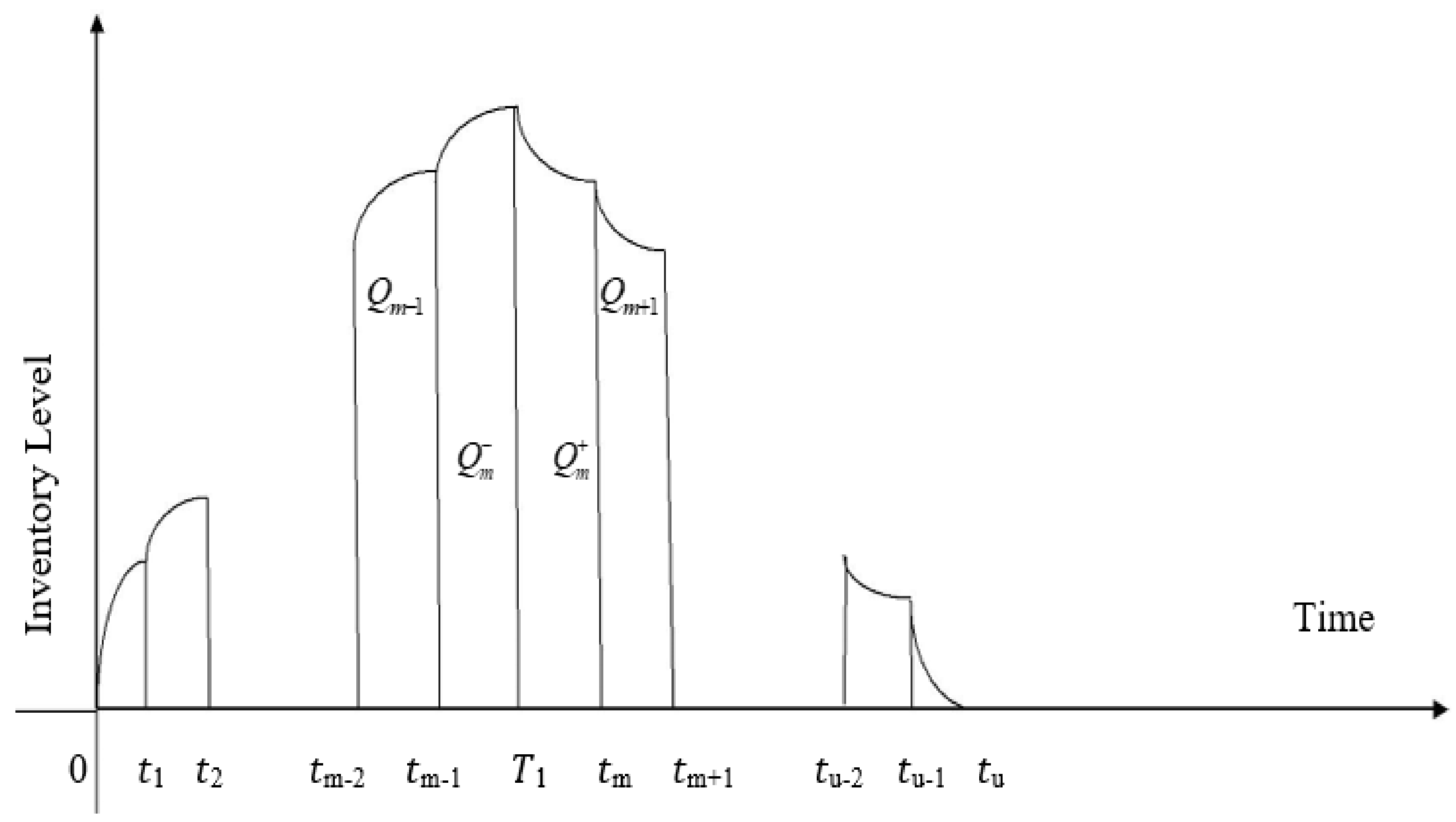
3.1. Finished Products of the Manufactures for the Given Inventory Model

The transformation rate of inventory situation throughout constructive stock in a time interval $[t_{q-1},t_q]$ and $[t_{m-1},T_1]$ is administered by the succeeding differential equations.

$$\frac{d{Q}_q(t)}{dt}+{\theta }_p{Q}_q(t)=p-(d_q-{\mathrm{as}}_q{) ; t}_{q-1}\le t\le t_q\hspace{1em}q=1,2,3, \dots ,m-1$$

(1)

$$\frac{Q{I}_m^{-}(t)}{dt}+{\theta }_p{Q}_m^{-}(t)=p-(d_m-{\mathrm{as}}_m{) ; t}_{m-1}\le t\le T_1$$

(2)

$$\mathrm{with} Q_1(0)=0,\hspace{1em}{Q}_q(t_{q-1})=Q_{q-1}(t_{q-1}) \& Q_m^{-}(t_{q-1})=Q_{m-1}(t_{q-1})$$

(3)

The frequency of revolution of inventory throughout stock-in situation $[T_1,t_m]$ and $[t_{j-1},t_j]$ is administrated by the resulting differential equations.

$$\frac{d{Q}_m^{+}(t)}{dt}+{\theta }_p{Q}_m^{+}(t)=-(d_m-{\mathrm{as}}_m{) ; T}_1\le t\le t_m$$

(4)

$$\frac{d{Q}_j(t)}{dt}+{\theta }_p{Q}_j(t)=-(d_j-{\mathrm{as}}_j{) ; t}_{j-1}\le t\le t_j\hspace{1em}j=m+1,m+2, \dots ,u$$

(5)

$$\mathrm{with}\hspace{1em}{Q}_{j-1}(t_{j-1})=Q_j(t_{j-1}) , Q_m^{+}(t_{m-1})=Q_m(T_{m-1})\hspace{1em}\&\hspace{1em}{Q}_u(t_u)=0,$$

(6)

Solving Equations (1) and (2) with the help of condition (3) is:

$$Q_q(t)=\frac{p-(d_q-{\mathrm{as}}_q)-p{e}^{-{\theta }_{p}t}}{{\theta }_p}+{\displaystyle \sum _{i=1}^q\frac{\left\{(d_i-d_{i-1})-a(s_i-s_{i-1})\right\}}{{\theta }_p}}{e}^{-{\theta }_p(t-t_{i-1})} ; t_{q-1}\le t\le t_k , q=1,2,3,\dots ,m-1$$

(7)

$$Q_m^{-}(t)=\frac{p-(d_m-a{s}_m)-p{e}^{-{\theta }_{p}t}}{{\theta }_p}+{\displaystyle \sum _{i=1}^m\frac{\left\{(d_i-d_{i-1})-a(s_i-s_{i-1})\right\}}{{\theta }_p}}{e}^{-{\theta }_p(t-t_{i-1})} ; t_{m-1}\le t\le T_1$$

(8)

An answer of the (stage 2) from the differential conditions (4) and (5) utilizing limit condition (6) is:

$$Q_m^{+}(t)=\frac{-(d_m-a{s}_m)}{{\theta }_p}+\frac{d_u{e}^{-{\theta }_p(t-t_u)}}{{\theta }_p}-{\displaystyle \sum _{i=m+1}^u\frac{\left\{(d_i-d_{i-1})-a(s_i-s_{i-1})\right\}}{{\theta }_p}}{e}^{-{\theta }_p(t-t_{i-1})}; T_1\le t\le t_m$$

(9)

$$Q_j(t)=\frac{-(d_j-a{s}_j)}{{\theta }_p}+\frac{d_u{e}^{-{\theta }_p(t-t_u)}}{{\theta }_p}-{\displaystyle \sum _{j=j+1}^u\frac{\left\{(d_i-d_{i-1})-a(s_i-s_{i-1})\right\}}{{\theta }_p}}{e}^{-{\theta }_p(t-t_{i-1})};$$

(10)

$$t_{j-1}\le t\le t_j, j=m+1, m+2,\dots , u$$

Using continuity condition at t = $T_1$, we have:

$$\begin{array}{l}\left[\frac{p-(d_m-a{s}_m)-p{e}^{-{\theta }_{p}t}}{{\theta }_p}+{\displaystyle \sum _{i=1}^m\frac{\left\{(d_i-d_{i-1})-a(s_i-s_{i-1})\right\}}{{\theta }_p}}{e}^{-{\theta }_p(t-t_{i-1})}=\right.\\ \left.\frac{-(d_m-a{s}_m)}{{\theta }_p}+\frac{d_u{e}^{-{\theta }_p(t-t_u)}}{{\theta }_p}-{\displaystyle \sum _{i=m+1}^u\frac{\left\{(d_i-d_{i-1})-a(s_i-s_{i-1})\right\}}{{\theta }_p}}{e}^{-{\theta }_p(t-t_{i-1})}\right]\end{array}$$

(11)

After simplification and ignoring the advanced power of ${\theta }_p$, we then get

$$T_1=\frac{1}{{\theta }_p}ln\left[\frac{\left(d_u-a{s}_u\right)e^{({\theta }_p) t_u}-{\displaystyle \sum _{i=1}^u\left(\left(d_i-d_{i-1}\right)-a\left(s_i-s_{i-1}\right)\right)e^{({\theta }_p) t_{i-1}}}}{p}+1\right]=\frac{1}{p}\left(A+\frac{{\theta }_{p}B}{2}\right)$$

(12)

where $A={\displaystyle \sum _{i=1}^u(d_i-a{s}_i)\left(t_i-t_{i-1}\right)}$ and $B={\displaystyle \sum _{i=1}^u\left(d_i-a{s}_i\right)\left(t_i^2-t_{i-1}^2\right)}$.

It is observed that Equation (12) are not related with $m$. Hence, the value of $t_i$ and $(d_i-a{s}_i)$ are recognized then the most delicate production time $T_1$ can originate directly by via Equation (12).

3.2. Calculation of Cost for Finished Products

Set up cost

$$T{S}_c=k_0$$

(13)

Time-dependant holding cost for finished products as follows;

$$\begin{gathered} T{H}_p=\left[\begin{array}{l}{h}_p\left({\displaystyle \sum _{k=1}^{m-1}{Q}_q}(t)+Q_m^{-}(t)+Q_m^{+}(t)+{\displaystyle \sum _{j=m+1}^u{Q}_j(t)}\right)\\ +h_{pp}t\left({\displaystyle \sum _{k=1}^{m-1}{Q}_q}(t)+Q_m^{-}(t)+Q_m^{+}(t)+{\displaystyle \sum _{j=m+1}^u{Q}_j(t)}\right)\end{array}\right] \\ T{H}_p=\left[\frac{h_{p}B}{2}+h_{pp}\left\{\begin{array}{l}-\frac{B}{2{\theta }_p}-C\left(\frac{A}{p{\theta }_p}+\frac{B}{2p}\right)+\frac{D}{{\theta }_{{}_p}^2}+\frac{A^2\mathrm{BE}}{p^2}+\frac{A^3}{2p^2}+\\ \frac{{3A}^{2}B{\theta }_p}{4p^2}+\left(d_u-{\mathrm{as}}_u\right)\left(\frac{{\theta }_{p}B{t}_u}{2p}+\frac{A{t}_u}{p^2}-\frac{AB}{p^2}\right)\end{array}\right\}\right] \end{gathered}$$

(14)

where $C={\displaystyle \sum _{i=1}^u\left\{\left(d_i-d_{i-1}\right)-a\left(s_i-s_{i-1}\right)\right\}{t}_{i-1}}$, $D={\displaystyle \sum _{i=1}^u\left\{\left(d_i-d_{i-1}\right)-a\left(s_i-s_{i-1}\right)\right\}(t_i-t_{i-1})}$ and $E={\displaystyle \sum _{i=1}^u\left\{\left(d_i-d_{i-1}\right)-a\left(s_i-s_{i-1}\right)\right\}}$.

The deterioration cost of finished products

$$T{D}_p=c_p\left\{p{T}_1-{\displaystyle \sum _{i=1}^u(d_i-a{s}_i)(t_i-t_{i-1})}\right\}=c_p\left\{A+\frac{{\theta }_{p}B}{2}-A\right\}=\frac{c_p{\theta }_{p}B}{2}$$

(15)

Preservation cost of finished products

$$P{T}_c=\xi T_1$$

(16)

The total cost of finished products $T{C}_p=T{S}_c+T{H}_p+T{D}_p+P{T}_c$

$$T{C}_p=\left[\begin{array}{l}{k}_0+\left\{\frac{h_{p}B}{2}+h_{pp}\left(-\frac{B}{2{\theta }_p}-C\left(\frac{A}{p{\theta }_p}+\frac{B}{2p}\right)+\frac{D}{{\theta }_p^2}+\frac{A^{2}BE}{p^2}+\frac{A^3}{2p^2}+\right.\right.\\ \left.\left.\frac{3A^{2}B{\theta }_p}{4p^2}+\left(d_u-a{s}_u\right)\left(\frac{{\theta }_{p}B{t}_u}{2p}+\frac{A{t}_u}{p}-\frac{AB}{p^2}\right)\right)\right\}+\frac{c_p{\theta }_{p}B}{2}+\xi T_1\end{array}\right]$$

(17)

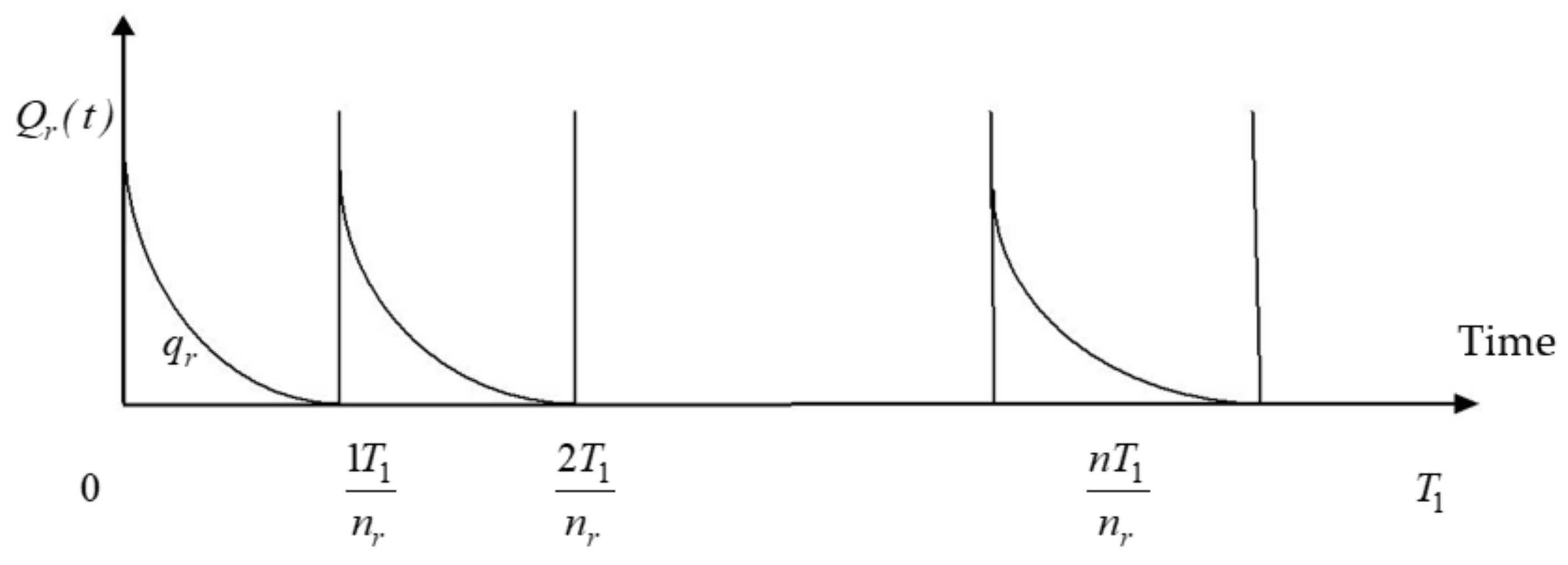
3.3. Manufactories’ Warehouse Raw Materials Inventory Model

The inventory level of raw quantifiable reaches zero due to deterioration and consumption of demand at time $t=\frac{T_1}{n_r}$, which can be formulated as;$\frac{d{Q}_r(t)}{dt}+{\theta }_r{Q}_r(t)=-f*p ; 0\le t\le \frac{T_1}{n_r}$. Using the boundary condition

$$I_r\left(\frac{T_1}{n_r}\right)=0$$

(18)

we have

$$Q_r=\frac{fp}{{\theta }_r}\left[e^{-{\theta }_r\left(t-\frac{T_1}{n_r}\right)}-1\right]=\frac{fp}{{\theta }_r}\left[e^{{\theta }_r\frac{T_1}{n_r}}\left(1-{\theta }_{r}t+\frac{{\left({\theta }_{r}t\right)}^2}{2}-\dots \right)-1\right]0\le t\le \frac{T_1}{n_r}$$

(19)

With the help of another boundary condition According to Figure 3 $Q_r\left(0\right)=q_r$ the lot size-for every delivery $q_r$ from supplier to manufacture becomes

$$\begin{gathered} q_r=\frac{fp}{{\theta }_r}\left[e^{{\theta }_r\left(\frac{T_1}{n_r}\right)}-1\right]\Rightarrow \frac{q_r{\theta }_r}{fp}=\left[e^{{\theta }_r\left(\frac{T_1}{n_r}\right)}-1\right] \\ \Rightarrow \left[\frac{q_r{\theta }_r}{fp}+1=e^{{\theta }_r\left(\frac{T_1}{n_r}\right)}\right]\Rightarrow \frac{1}{{\theta }_r}Log\left[1+\frac{q_r{\theta }_r}{fp}\right]=\left(\frac{T_1}{n_r}\right) \\ {T}_1=\frac{n_r}{{\theta }_r}Log\left[1+\frac{q_r{\theta }_r}{fp}\right]=\frac{n_r}{{\theta }_r}\left\{\frac{q_r{\theta }_r}{fp}-\frac{{\left(\frac{q_r{\theta }_r}{fp}\right)}^2}{2}+\frac{{\left(\frac{q_r{\theta }_r}{fp}\right)}^3}{3}-\frac{{\left(\frac{q_r{\theta }_r}{fp}\right)}^4}{4}+,\hspace{0.17em}\dots \right\} \end{gathered}$$

(20)

Here, $T_1$ is term of $q_r$ to find the optimal value of decision variable $q_r$.

3.4. Raw Materials Cost Calculation

• The ordering cost:

  $$T{O}_r=s_r{n}_r$$

  (21)
• Transportation cost of raw materials:

  $$Ctran=c_t\hspace{0.17em}{q}_r$$

  (22)
• The holding cost of raw material:$\mathit{THr}$

  $$T{H}_r=n_r{h}_r{\displaystyle \underset{0}{\overset{\frac{T_1}{n_r}}{\int }}t{Q}_r(t)} dt=n_r{h}_r{\displaystyle \underset{0}{\overset{\frac{T_1}{n_r}}{\int }}\frac{t\hspace{0.17em}fp}{{\theta }_r}\left\{e^{{\theta }_r\left(\frac{T_1}{n_r}-t\right)}-1\right\}} dt=\frac{f{h}_r}{3p^2{n}_r^2}\left[\frac{A^3}{2}+\frac{3A^{2}B{\theta }_p}{4}+\frac{A^4{\theta }_r}{p{n}_r}\right]$$

  (23)
• The deterioration cost of raw material:

  $$T{D}_r=c_r\left(n_r{q}_r-fp{T}_1\right)=c_r\left(\frac{n_{r}fp}{{\theta }_r}\left(e^{{\theta }_r\left(\frac{T_1}{n_r}\right)}-1\right)-fp{T}_1\right)=\frac{f{c}_r{\theta }_r}{2p{n}_r}\left[A^2{+\theta }_{p}AB\right]=\frac{f{c}_r{\theta }_r{A}^2}{2p{n}_r}$$

  (24)
• The preservation technology cost of raw material:

  $$PT{C}_r=\xi \frac{T_1}{n_r}=\frac{\xi }{{\theta }_r}\left(\frac{q_r{\theta }_r}{fp}-\frac{{\left(\frac{q_r{\theta }_r}{fp}\right)}^2}{2}+\frac{{\left(\frac{q_r{\theta }_r}{fp}\right)}^3}{3}-\frac{{\left(\frac{q_r{\theta }_r}{fp}\right)}^4}{4}\right)$$

  (25)

The total cost of raw material: $T{C}_r={\mathrm{TO}}_r+Ctran+T{H}_r +T{D}_r+PT{C}_r$

$$T{C}_r(n_r,\xi ,q_r)=\left[\begin{array}{l}{s}_r{n}_r+c_t\hspace{0.17em}{q}_r+\frac{f{h}_r}{3p^2{n}_r^2}\left\{\frac{A^3}{2}+\frac{{3A}^2{B\theta }_p}{4}+\frac{A^4{\theta }_r}{{pn}_r}\right\}+\frac{{\mathrm{fc}}_r{\theta }_r{A}^2}{2p{n}_r}\\ +\frac{\xi }{{\theta }_r}\left(\frac{q_r{\theta }_r}{fp}-\frac{{\left(\frac{q_r{\theta }_r}{fp}\right)}^2}{2}+\frac{{\left(\frac{q_r{\theta }_r}{fp}\right)}^3}{3}-\frac{{\left(\frac{q_r{\theta }_r}{fp}\right)}^4}{4}\right)\end{array}\right]$$

(26)

3.5. Model 2: Modal with Shortage Allowed

Model/-2 is similar to model-1; the demand rate $(d_i-a{s}_i)$ associated with $i^{th}$ the market is supplied in the time interval $[t_{i-1},t_i]for i=1,2,3,\dots ,n$, where $t_u$ just the time that it reaches to a shortage in the time interval $[t_{i-1},t_i]$ for $i=u+1,u+2,\dots ,n$ demands arrive with rate $d_{i-1}$. This means that inventory at time $t_u$ is zero and before this time, it will always be an optimistic value.

3.5.1. Manufacture Is Finished Products, Inventory Model

Let $(d_i-a{s}_i)$ and $t_i$$(i=1,2,3,\dots ,u)$ be the demand rate of i^th market and the time that demand changes, respectively. Demand rate $(d_i-a{s}_i)$ associate with i^th market is supplied in the time interval $[t_{i-1},t_i]for i=1,2,3,\dots ,u$. Here, $t_u$ is just the time that it encounters a shortage. This means that inventory at time $t_u$ is zero and before this time, it will always have a positive value. We suppose that production begins at time zero and just at this time the inventory goes to accumulate until the end of production time that is $T_1$. Then, after time $T_1$, the inventory declines due to both of consumption and deterioration (see Figure 4). For obtaining the maximum benefit, the manufacture must determine the value of $T_1$. After $t_u$ the producer who has purchased all the backlogged demands via a subcontract, will compensate them. The only difference with Model 1 is that shortages are allowed in Model 2 and fulfilled by backlogging.

The producer will compensate those demands that have purchased the backlogged demands via a subcontract after the time $t_u$ up to the time $T=t_{u+1}$ at the end of each cycle. The shortage will reach the maximum value. In Phases 1 and Phase 2 of Model 2, all the calculations are the same as those in Model 1, since in both the model at time $t=t_u$ the inventory reduced to zero, the only difference is that in (Model 1) the total period of a cycle $T=t_u$, where the inventory reduces to zero only but in Model 2 the total time period of a cycle $T=t_{u+1}$, when the shortage will reach to its maximum values and the insufficient demand is practically backlogged by the manufacturer via a subcontract.

Hence, the inventory level in the time interval $t_u\le t\le T$ is given as:

$$Q_{z+1}=-(d_z-a{s}_z)(t-t_z)+{\displaystyle \sum _{i=u}^{z-1}(d_i-a{s}_i)\left(t_{i+1}-t_i\right);t_z\le t\le t_{z+1},z=u+1,u+2,\dots ,n}$$

(27)

The maximum shortage has been full field

$$\begin{gathered} Q_{z+1}={\displaystyle \underset{t_z}{\overset{t_{z+1}}{\int }}\left(-(d_z-a{s}_z)(t-t_z)-{\displaystyle \sum _{i=u}^{z-1}(d_i-a{s}_i)\left(t_{i+1}-t_i\right)}\right)}dt ; t_z\le t\le t_{z+1},z=u+1,u+2,\dots ,n \\ {Q}_{z+1}=-\left(\frac{(d_z-a{s}_z)}{2}{\left(t_{z+1}-t_z\right)}^2+\left(t_{z+1}-t_z\right){\displaystyle \sum _{i=u}^{z-1}(d_i-a{s}_i)\left(t_{i+1}-t_i\right)}\right);t_z\le t\le t_{z+1} \end{gathered}$$

(28)

3.5.2. Cost Calculation

Similar to Model 1 the holding cost $T{H}_p$, the deterioration cost $T{D}_p$ and the preservation technology cost $PT{C}_p$ of finished products are the same but the backlogging cost of finished products $T{S}_p$ and purchase cost of finished products $T{B}_p$ are as follows:

The purchase cost of finished products $T{S}_p$:

$$T{S}_p=\beta c_{fc}{\displaystyle \sum _{z=u}^n{I}_{z+1}}=-\beta c_{fc}\left({\displaystyle \sum _{i=u}^{z-1}{\displaystyle \sum _{z=u}^n(d_i-a{s}_i)(t_{i+1}-t_i)\left(t_{z+1}-t_z\right)+{\displaystyle \sum _{z=u}^{z=n}\frac{(d_z-a{s}_z)}{2}{\left(t_{z+1}-t_z\right)}^2}}}\right)$$

(29)

The backlogging cost of finished products $T{B}_p$:

$$T{B}_p=-c_b\beta {\displaystyle \sum _{z=u}^n{I}_{z+1}}=c_b\beta \left({\displaystyle \sum _{i=u}^{z-1}{\displaystyle \sum _{z=u}^n(d_i-a{s}_i)(t_{i+1}-t_i)\left(t_{z+1}-t_z\right)+{\displaystyle \sum _{z=u}^{z=n}\frac{(d_z-a{s}_z)}{2}{\left(t_{z+1}-t_z\right)}^2}}}\right)$$

(30)

Hence, the total cost of finished products is $T{C}_p=k_0+T{H}_p+T{D}_p+PT{C}_p+T{S}_p+T{B}_p$

$$T{C}_p(n_r,\xi ,q_r)=\left[\begin{array}{cc}\hfill & k_0+\frac{h_{p}B}{2}+h_{pp}\left\{-\frac{B}{2{\theta }_p}-C\left(\frac{A}{p{\theta }_p}+\frac{B}{2p}\right)+\frac{D}{{\theta }_p^2}+\frac{A^{2}BE}{p^2}+\frac{A^3}{2p^2}+\frac{3A^{2}B{\theta }_p}{4p^2}+\right.\hfill \\ \hfill & \left.\left(d_u-a{s}_u\right)\left(\frac{{\theta }_{p}B{t}_u}{2p}+\frac{A{t}_u}{p}-\frac{AB}{p^2}\right)\right\}+\frac{c_p{\theta }_{p}B}{2}+\xi \left(A+\frac{{\theta }_{p}B}{2}\right)+\beta (c_b-c_{fc})\hfill \\ \hfill & \left(\sum _{i=u}^{z-1}\sum _{z=u}^n(d_i-a{s}_i)(t_{i+1}-t_i)\left(t_{z+1}-t_z\right)+\sum _{z=u}^{z=n}\frac{(d_z-a{s}_z)}{2}{\left(t_{z+1}-t_z\right)}^2\right)\hfill \end{array}\right]$$

(31)

3.5.3. Integrated Inventory Model-2 and Solution

The total cost of finished products goods and total cost of raw materials for the model-2 is $TC=T{C}_p+T{C}_r$:

$$TC(n_r,\xi ,q_r)=\left[\begin{array}{cc}\hfill & k_0+\frac{h_{p}B}{2}+h_{pp}\left\{-\frac{B}{2{\theta }_p}-C\left(\frac{A}{p{\theta }_p}+\frac{B}{2p}\right)+\frac{D}{\theta {}_p^2}+\frac{A^{2}BE}{p^2}+\frac{A^3}{2p^2}+\frac{3A^{2}B{\theta }_p}{4p^2}+\right.\hfill \\ \hfill & \left.\left(\frac{{\theta }_{p}B{t}_u}{2p}+\frac{A{t}_u}{p}-\frac{\mathit{AB}}{p^2}\right)\left(d_u-a{s}_u\right)\right\}+\frac{c_p{\theta }_{p}B}{2}+\xi \left(A+\frac{{\theta }_{p}B}{2}\right)+\beta (c_b-c_{fc})\hfill \\ \hfill & \left(\sum _{i=u}^{z-1}\sum _{z=u}^n(d_i-a{s}_i)(t_{i+1}-t_i)\left(t_{z+1}-t_z\right)+\sum _{z=u}^{z=n}\frac{(d_z-a{s}_z)}{2}{\left(t_{z+1}-t_z\right)}^2\right)+\hfill \\ \hfill & s_r{n}_r+c_t{q}_r+\frac{f{h}_r}{3p^2{n}_r^2}\left\{\frac{A^3}{2}+\frac{3A^{2}B{\theta }_p}{4}+\frac{A^4{\theta }_r}{p{n}_r}\right\}+\frac{f{c}_r{\theta }_r{A}^2}{2p{n}_r}+\hfill \\ \hfill & \frac{\xi }{{\theta }_r}\left(\frac{q_r{\theta }_r}{fp}-\frac{1}{2}{\left(\frac{q_r{\theta }_r}{fp}\right)}^2+\frac{1}{3}{\left(\frac{q_r{\theta }_r}{fp}\right)}^3-\frac{1}{4}{\left(\frac{q_r{\theta }_r}{fp}\right)}^4\right)\hfill \end{array}\right]$$

(32)

4. Objective (Cost Calculation of Raw Material and Manufacture Finished Products)

The goal of this study is to invent the optimal rate of cost of preservation ${\xi }^{*}$(decision variable) for both the model that minimizes the whole cost TC is as follows Put ${\theta }_p={\theta }_2{e}^{-\alpha \xi } \mathrm{and} {\theta }_r={\theta }_1{e}^{-\alpha \xi }$; then, the equation reduces to $TC$ as follows;

$$TC(n_r,\xi ,q_r)=\left[\begin{array}{cc}\hfill & k_0+\frac{h_{p}B}{2}+h_{\mathit{pp}}\left\{-\frac{B{e}^{\alpha \xi }}{2{\theta }_2}-C\left(\frac{A{e}^{\alpha \xi }}{p{\theta }_2}+\frac{B}{2p}\right)+\frac{D{e}^{2\alpha \xi }}{\theta {}_2^2}+\frac{A^2\mathit{BE}}{p^2}+\frac{3A^{2}B{\theta }_2{e}^{-\alpha \xi }}{4p^2}+\frac{A^3}{2p^2}\right.\hfill \\ \hfill & \left.+\left(d_u-a{s}_u\right)\left(\frac{{\theta }_2{e}^{-\alpha \xi }B{t}_u}{2p}+\frac{A{t}_u}{p}-\frac{\mathit{AB}}{p^2}\right)\right\}+\frac{c_p{\theta }_2{e}^{-\alpha \xi }B}{2}+\xi \left(A+\frac{{\theta }_2{e}^{-\alpha \xi }B}{2}\right)+\hfill \\ \hfill & \beta \left(c_b-c_{\mathit{fc}}\right)\left(\sum _{i=u}^{z-1}\sum _{z=u}^n(d_i-a{s}_i\left)\right(t_{i+1}-t_i)\left(t_{z+1}-t_z\right)+\sum _{z=u}^{z=n}\frac{(d_z-a{s}_z)}{2}{\left(t_{z+1}-t_z\right)}^2\right)\hfill \\ \hfill & +s_r{n}_r+c_t{q}_r+\frac{f{h}_r}{3p^2{n}_r^2}\left\{\frac{A^3}{2}+\frac{3A^{2}B{\theta }_2{e}^{-\alpha \xi }}{4}+\frac{A^4{\theta }_1{e}^{-\alpha \xi }}{p{n}_r}\right\}+\frac{f{c}_r{\theta }_1{e}^{-\alpha \xi }{A}^2}{2p{n}_r}+\frac{\xi }{{\theta }_1{e}^{-\alpha \xi }}\hfill \\ \hfill & \left(\frac{q_r{\theta }_1{e}^{-\alpha \xi }}{fp}-\frac{1}{2}{\left(\frac{q_r{\theta }_1{e}^{-\alpha \xi }}{fp}\right)}^2+\frac{1}{3}{\left(\frac{q_r{\theta }_1{e}^{-\alpha \xi }}{fp}\right)}^3-\frac{1}{4}{\left(\frac{q_r{\theta }_1{e}^{-\alpha \xi }}{fp}\right)}^4\right)\hfill \end{array}\right]$$

(33)

Differentiate with respect to $\xi$

$$\frac{\partial TC(n_r,\xi ,q_r)}{\partial \xi }=\left[\begin{array}{cc}\hfill & h_{\mathit{pp}}\left(-\frac{\alpha B{e}^{\alpha \xi }}{2{\theta }_2}-\frac{\alpha A{e}^{\alpha \xi }C}{p{\theta }_2}+\frac{2\alpha e^{2\alpha \xi }D}{\theta {}_2^2}-\frac{3\alpha A^{2}B{\theta }_2{e}^{-\alpha \xi }}{4p^2}-\frac{\left(d_u-a{s}_u\right)t_u\alpha B{\theta }_2{e}^{-\alpha \xi }}{2p}\right)\hfill \\ \hfill & -\frac{\alpha c_{p}B{\theta }_2{e}^{-\alpha \xi }}{2}+A+\frac{B{\theta }_2{e}^{-\alpha \xi }}{2}-\frac{\alpha f{h}_r{A}^{2}B{\theta }_2{e}^{-\alpha \xi }}{12p^2{n}_r^2}-\frac{\alpha f{h}_r{A}^4{\theta }_1{e}^{-\alpha \xi }}{3p^3{n}_r^3}-\frac{\alpha f{c}_r{A}^2{\theta }_1{e}^{-\alpha \xi }}{2p{n}_r}\hfill \\ \hfill & +\frac{A}{p{n}_r}+\frac{e^{-2\alpha \xi }{q}_r\left(6e^{2\alpha \xi }{f}^2{p}^2+2q_r^2{\theta }_1^2\left(1-2\alpha \xi \right)+3e^{\alpha \xi }fp{q}_r{\theta }_1(\alpha \xi -1)\right)}{6f^3{p}^3}\hfill \end{array}\right]$$

(34)

$$\frac{{\partial }^{2}TC(n_r,\xi ,q_r)}{\partial {\xi }^2}=\left[\begin{array}{l}{h}_{pp}(-\frac{{\alpha }^2{Be}^{\alpha \xi }}{{2\theta }_2}-\frac{{\alpha }^2{Ae}^{\alpha \xi }C}{{p\theta }_2}+\frac{{4\alpha }^2{e}^{2\alpha \xi }D}{{\theta }_2^2}+\frac{{3\alpha }^2{A}^2{B\theta }_2{e}^{-\alpha \xi }}{{4p}^2}+\left(d_u-{\mathrm{as}}_u\right)\\ \frac{t_u{\alpha }^2{B\theta }_2{e}^{-\alpha \xi }}{2p})+\frac{{\alpha }^2{c}_p{B\theta }_2{e}^{-\alpha \xi }}{2}+\frac{{\alpha }^2{fh}_r{A}^2{B\theta }_2{e}^{-\alpha \xi }}{{12p}^2{n}_r^2}+\frac{{\alpha }^2{fh}_r{A}^4{\theta }_1{e}^{-\alpha \xi }}{{3p}^3{n}_r^3}+\\ \frac{{\alpha }^2{fc}_r{A}^2{\theta }_1{e}^{-\alpha \xi }}{{2pn}_r}+\frac{{\alpha }^2{\xi B\theta }_2{e}^{-\alpha \xi }}{{2pn}_r}+\frac{e^{-2\alpha \xi }{q}_r^2\alpha {\theta }_1\left\{{3e}^{\alpha \xi }fp\left(\alpha \xi -2\right)+8q_r{\theta }_1\left(\alpha \xi -1\right)\right\}}{6f^3{p}^3}\end{array}\right]$$

$$\frac{{\partial }^2\mathit{TC}(n_r,\xi ,q_r)}{\partial {\xi }^2}=\left[\begin{array}{cc}\hfill & h_{\mathrm{pp}}\left\{\begin{array}{cc}\hfill & \frac{{\alpha }^2{e}^{\alpha \xi }}{{\theta }_2}\left(\frac{2D{e}^{\alpha \xi }}{{\theta }_2}-\frac{AC}{p}\right)+\frac{{\alpha }^2{e}^{\alpha \xi }}{{\theta }_2}\left(\frac{2e^{\alpha \xi }D}{{\theta }_2}+\frac{B}{2}\right)\hfill \\ \hfill & +\frac{3{\alpha }^2{A}^{2}B{\theta }_2{e}^{-\alpha \xi }}{4p^2}+\frac{\left(d_u-a{s}_u\right)t_u{\alpha }^{2}B{\theta }_2{e}^{-\alpha \xi }}{2p}\hfill \end{array}\right\}+\hfill \\ & \frac{{\alpha }^{2}f{h}_r{A}^{2}B{\theta }_2{e}^{-\alpha \xi }}{12p{n}_r}+\alpha B{\theta }_2{e}^{-\alpha \xi }\left(\frac{\alpha c_p}{2}-\frac{1}{p{n}_r}\right)+\frac{{\alpha }^{2}f{h}_r{A}^4{\theta }_1{e}^{-\alpha \xi }}{3p^2{n}_r^2}\hfill \\ & +\frac{{\alpha }^{2}f{c}_r{A}^2{\theta }_1{e}^{-\alpha \xi }}{2p{n}_r}+\frac{{\alpha }^2\xi B{\theta }_2{e}^{-\alpha \xi }}{2p{n}_r}+\frac{3e^{-\alpha \xi }{q}_r^2\alpha {\theta }_{1}fp}{6f^3{p}^3}\left(\alpha \xi -2\right)+\hfill \\ & +\frac{e^{-2\alpha }{q}_r^3\alpha 8q_r{\theta }_1^2}{6f^3{p}^3}\left(\alpha \xi -1\right)\hfill \end{array}\right]$$

(35)

$\frac{{\partial }^{2}TC(n_r,\xi ,q_r)}{\partial {\xi }^2}>0$ If $\left(\frac{{2\mathit{De}}^{\alpha \xi }}{{\theta }_2}-\frac{\mathit{AC}}{p}\right)>0,\left(\frac{\alpha c_p}{2}-\frac{1}{p{n}_r}\right)>0,\left(\alpha \xi -2\right)>0\&\left(\alpha \xi -1\right)>0$.

To find the optimal value of another decision variable $q_r$, differentiate total cost function with respect to $q_r$; then, we get:

$$\frac{\partial TC(n_r,\xi ,q_r)}{\partial q_r}=\left[c_t+\frac{1}{{\theta }_r}\left(\frac{{\theta }_r}{fp}-\frac{q_r{\theta }_r^2}{f^2{p}^2}+\frac{q_r^2{\theta }_r^3}{f^3{p}^3}-\frac{q_r^3{\theta }_r^4}{f^4{p}^4}\right)\xi \right]$$

(36)

Again, differentiate with respect to $q_r$:

$$\frac{{\partial }^{2}TC(n_r,\xi ,q_r)}{\partial q_r^2}=\left[\left(-\frac{{\theta }_r}{f^2{p}^2}+\frac{2q_r{\theta }_r^2}{f^3{p}^3}-\frac{3q_r^2{\theta }_r^3}{f^4{p}^4}\right)\xi \right]$$

(37)

Due to the highly nonlinearity of the objective function, it is not easy to find the closed-form solution. In this context, to solve this model, Mathematica software is used and we get $\frac{{\partial }^{2}TC(n_r,\xi ,q_r)}{\partial q_r^2}>0$.

Now, using the hessian matrix of order (2 × 2) $\left[\begin{array}{l}\frac{{\partial }^{2}TC(\xi ,q_r)}{\partial {\xi }^2}\hspace{0.17em}\hspace{0.17em}\hspace{0.17em}\hspace{0.17em}\hspace{0.17em}\hspace{0.17em}\hspace{0.17em}\frac{{\partial }^{2}TC(\xi ,q_r)}{\partial \xi \partial q_r}\\ \frac{{\partial }^{2}TC(\xi ,q_r)}{\partial q_r\partial \xi }\hspace{0.17em}\hspace{0.17em}\hspace{0.17em}\hspace{0.17em}\hspace{0.17em}\hspace{0.17em}\frac{{\partial }^{2}TC(\xi ,q_r)}{\partial q_r^2}\end{array}\right]>0$,

Thus, cost function is positive definite. So, the function has a minimum value.

The optimal value of decision variable ${\xi }^{*} \& \hspace{0.17em}{q}_r^{*}$ is obtained with the help of Mathematica-software-9 from the Equations (34) and (36). The subsequent neutral of this investigation is to regulate the optimal value of a total number of deliveries $n_r^{*}$; the manufactories’ warehouse raw materials inventory model is the same for Model 1 and Model 2, therefore, the value of $n_r^{*}$, which minimizes TC, where $n_r$ a discrete variable is as follows differentiated with respect to $n_r$.

The optimal cost of the over-all number of deliveries $n_r^{*}$ is

$$TC(n-1)<TC(n)\hspace{0.17em}\hspace{1em}\& TC(n)>TC(n+1)$$

(38)

From Equation (38), the optimal value of a total number of deliveries $n_r^{*}$ is obtained.

5. Experimental Analysis

Example 1: He et al. [34] associated statistics of the situation with three-market circumstances with the measures of Proposition 1, the following facts are measured as designed to authenticate the suggested Model 1 and Model 2. Let us consider a food processing farm situated in Ranchi. The rate of demand for the processed food in the marketplace one is 20 units per week while for the market two is 38 units per calendar week and the demand frequency of bazaar three stands at 18 units per week. The selling spells of market one is USD 8/unit, market two is USD 20/unit and for market three is USD 12/unit. The amount of production is 150 units per week. The selling season of the leading market is from calendar week 1 to week 8 and for 2nd market is from week 8 to week 20 and for the 3rd market is from week 20 to week 30. The crumbling pace of crude materials is USD 0.2 units each week, completed items is USD 0.3 units each week, the unit use of crude materials is USD 1.2 units per unit of the completed item the requesting cost of crude materials is USD 400 per request, the cost of setup for creation is USD 600, the unit cost of crude materials is USD 5, the costs of holding for raw materials is USD 0.1 per week and the cost of holding of finished goods is USD 0.15 per week and $h_{pp}=0.25$. The transportation cost of the raw material is USD 1.5 per trip. For the preservation parameter $\alpha =0.2$ and $a=0.5,\beta =0.5,{\theta }_2=0.1 \& {\theta }_1=0.3$ the component production cost is USD 10, respectively. The cost of shortage of final goods is USD 2 per week and the cost of purchase for finished products is USD 1.6 per week. The optimal production time $T_1$, the optimal lot—size per delivery from supplier to manufacture $q_r$, the optimal value of preservation technology (PT) cost $\xi$, the optimal number of raw materials distributions from provider to manufacture $n_r$, without and with shortage the optimal cost $TC$, with and lacking technology of preservation are intended with the assistance of Equations (12), (33), (34), (35), (37) and (39). From the above analyses, the optimal solution of $T_1$, $q_r$, $\xi$ and $n_r$, denoted by $T_1^{*}$, $q_r^{*}$, ${\xi }^{*}$ and $n_r^{*}$, which are shown in

Table 2. Optimal value of decision variables, dependent variable and total costs.

${\mathit{n}}_{\mathit{r}}^{*}$	With Preservation Technology					Without Preservation Technology
	${\mathit{\xi }}^{*}$	${\mathit{T}}_1^{*}$	${\mathit{q}}_{\mathit{r}}^{*}$	$\mathbf{Optimal} \mathbf{Cost} \mathit{T}\mathit{C}$		${\mathit{T}}_1^{*}$	${\mathit{q}}_{\mathit{r}}^{*}$	$\mathbf{Optimal} \mathbf{Cost} \mathit{T}\mathit{C}$
				Without Shortage	With Shortage			Without Shortage	With Shortage
2	6.23	20.33	3422	793,905	795,436	9.37	2282	731,044	732,575
3	6.25	20.33	3422	793,858	795,389	9.37	2282	731,303	732,834

.

Example 2: We take production time for the finished product is eight weeks under preservation technology or 20 weeks without preservation technology; then, the result will be shown below in

Table 3. Optimal value of different parameters and total costs.

${\mathit{n}}_{\mathit{r}}^{*}$	With Preservation Technology				Without Preservation Technology
	${\mathit{\xi }}^{*}$	${\mathit{q}}_{\mathit{r}}^{*}$	$\mathbf{Optimal} \mathbf{Cos}\mathbf{t} \mathit{T}\mathit{C}$		${\mathit{q}}_{\mathit{r}}^{*}$	$\mathbf{Optimal} \mathbf{Cos}\mathbf{t} \mathit{T}\mathit{C}$
			Without Shortage	With Shortage		Without Shortage	With Shortage
2	6.23	3206	793,452	794,926	2202	730,540	732,143
3	6.25	3206	793,402	794,845	2202	730,808	732,475

.

Compression of previous work data has been shown in

Table 4. Compression of previous work.

Optimal Values of Previous Work [34]			Optimal Values of This Paper
${\mathit{n}}_{\mathit{r}}^{*}$	${\mathit{T}}_1^{*}$	Total Cost (Without Shortage)	${\mathit{n}}_{\mathit{r}}^{*}$	${\mathit{T}}_1^{*}$	Total Cost (Without Shortage)
6	19.30	19,287	2	11.05	17,471
7	19.30	19,300	3	11.05	18,780

.

We make some change in the value of parameters $p=350,hp=0.05,{\theta }_p=0.4,$ ${\theta }_r=0.3 \& h_{pp}=0$ and other the same, then we get result shown below in Table 4.

In this paper, we reduce the optimal time $T_1^{*}$, number of deliveries of raw material $n_r^{*}$ and total cost $TC$ if we change some values of the parameter. We can say that this paper reduces optimal time, number of deliveries of raw material and total cost. Therefore, that industry adopts this model.

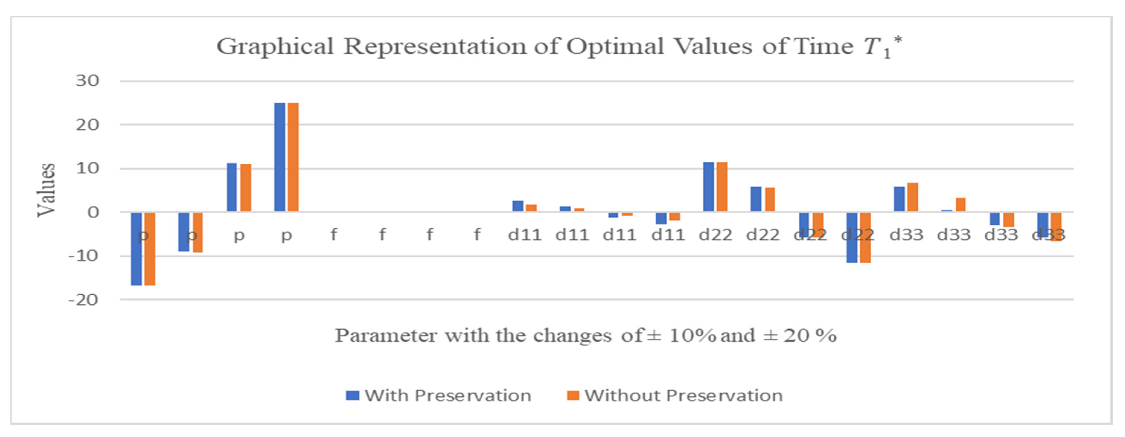
6. Sensitivity Analyses and Graphical Analysis

6.1. Sensitivity Analyses

To show the impact of differences in the various parameter of the proposed model (1 and 2), the post optimality analysis is carried out by considering -20% to 20% upsurge or reduction of one parameter and keeping other parameters same. The post optimality analysis is conceded out by altering the quantified parameter $p,f,(d_1-a{s}_1),(d_2-a{s}_2),(d_3-a{s}_3)$ $c_r,c_p,c_{b,} and c_{fc}$(Let $(d_1-a{s}_1)=d_{11},(d_2-a{s}_2)=d_{22},(d_3-a{s}_3)=d_{33}$) by

Table 5. Effect of changes of various parameter.

Parameter		With Preservation Technology						Without Preservation Technology
		${\mathit{\xi }}^{*}$	${\mathit{n}}_{\mathit{r}}^{*}$	${\mathit{T}}_1^{*}$	${\mathit{q}}_{\mathit{r}}^{*}$	Without and with Shortage		${\mathit{n}}_{\mathit{r}}^{*}$	${\mathit{T}}_1^{*}$	${\mathit{q}}_{\mathit{r}}^{*}$	Without and with Shortage
						$\mathit{T}{\mathit{C}}^{*}$	$\mathit{T}{\mathit{C}}^{*}$				$\mathit{T}{\mathit{C}}^{*}$	$\mathit{T}{\mathit{C}}^{*}$
$p$	20	4.00	−8.60	−16.63	−2.68	−29.51	−29.40	−8.82	−16.67	−4.89	−29.30	−29.18
	10	2.13	−4.59	−9.04	−1.47	−16.76	−16.70	−4.57	−9.10	−2.48	−16.64	−16.57
	−10	−2.38	5.42	11.12	1.84	22.65	22.57	5.48	11.07	2.66	22.48	22.39
	−20	−5.02	12.09	25.00	4.20	44.33	44.12	12.05	24.94	4.57	43.88	43.68
$f$	20	−0.20	8.75	0.00	20.00	0.26	0.26	9.34	0.00	20.00	0.06	0.06
	10	−0.05	5.42	0.00	10.00	0.13	0.13	4.71	0.00	10.00	0.03	0.03
	−10	0.05	−4.59	0.00	−10.00	−0.13	−0.13	−4.95	0.00	−10.00	−0.03	−0.03
	−20	0.11	−9.93	0.00	−20.00	−0.26	−0.26	−10.36	0.00	−20.00	−0.06	−0.06
$d_{11}$	20	−0.67	2.08	2.70	3.15	10.01	10.00	3.55	1.82	3.72	9.96	9.96
	10	−0.36	0.75	1.40	1.57	4.93	4.93	2.00	0.89	1.85	4.91	4.91
	−10	0.26	−0.59	−1.33	−1.56	−4.79	−4.78	−1.86	−0.93	−1.82	−4.76	−4.76
	−20	0.73	−1.92	−2.75	−3.12	−9.43	−9.43	−3.79	−1.87	−3.61	−9.38	−9.38
$d_{22}$	20	−2.84	6.08	11.48	13.59	37.71	37.61	11.66	11.46	24.90	37.38	37.28
	10	−1.45	3.41	5.79	6.74	17.84	17.79	5.86	5.71	11.89	17.69	17.64
	−10	1.51	−3.26	−5.72	−6.62	−15.92	−15.88	−5.73	−5.76	−10.87	−15.79	−15.75
	−20	3.22	−5.93	−11.53	−13.12	−30.04	−29.97	−11.52	−11.51	−20.80	−29.78	−29.71
$d_{33}$	20	−0.67	2.75	5.79	6.84	37.67	37.53	4.71	6.69	13.99	37.50	37.35
	10	−0.05	0.08	2.45	3.56	17.87	17.80	2.39	3.30	6.81	17.78	17.71
	−10	0.42	−1.26	−2.87	−3.37	−16.04	−15.98	−2.25	−3.34	−6.46	−15.96	−15.90
	−20	0.73	−2.59	−5.84	−6.72	−30.38	−30.26	−4.95	−6.69	−12.59	−30.22	−30.11
$c_r$	20	0.05	4.08	0.00	0.00	0.02	0.02	5.09	0.00	0.00	0.02	0.02
	10	0.05	2.08	0.00	0.00	0.01	0.01	2.39	0.00	0.00	0.01	0.01
	−10	−0.05	−1.26	0.00	0.00	−0.01	−0.01	−2.64	0.00	0.00	−0.01	−0.01
	−20	−0.05	−3.93	0.00	0.00	−0.02	−0.02	−5.34	0.00	0.00	−0.02	−0.02
$c_p$	20	−2.69	0.00	0.00	0.00	0.62	0.62	0.00	0.00	0.00	0.62	0.62
	10	−1.45	0.00	0.00	0.00	0.31	0.31	0.00	0.00	0.00	0.31	0.31
	−10	1.66	0.00	0.00	0.00	−0.31	−0.31	0.00	0.00	0.00	−0.31	−0.31
	−20	3.53	0.00	0.00	0.00	−0.62	−0.62	0.00	0.00	0.00	−0.62	−0.62
$b_f$	20	0.00	0.00	0.00	0.00	0.00	0.38	0.00	0.00	0.00	0.00	0.38
	10	0.00	0.00	0.00	0.00	0.00	0.19	0.00	0.00	0.00	0.00	0.19
	−10	0.00	0.00	0.00	0.00	0.00	−0.19	0.00	0.00	0.00	0.00	−0.19
	−20	0.00	0.00	0.00	0.00	0.00	−0.38	0.00	0.00	0.00	0.00	−0.38
$c_{fc}$	20	0.00	0.00	0.00	0.00	0.00	−0.31	0.00	0.00	0.00	0.00	−0.31
	10	0.00	0.00	0.00	0.00	0.00	−0.15	0.00	0.00	0.00	0.00	−0.15
	−10	0.00	0.00	0.00	0.00	0.00	0.15	0.00	0.00	0.00	0.00	0.15
	−20	0.00	0.00	0.00	0.00	0.00	0.31	0.00	0.00	0.00	0.00	0.31

shows the sensitivity of the numerous constraints on the optimum value of ${\xi }^{*},n_r^{*},T_1^{*}\&q_r^{*}$, without and with shortage total cost $T{C}^{*}$ of this study manifested the following facts:

A graphical representation of the sensitivity analysis has been shown in Figure 5, Figure 6, Figure 7, Figure 8, Figure 9 and Figure 10.

1. The optimal value of ${\xi }^{*}$ slightly change in the impost of parameters $f,d_{11} \& d_{33}$, moderately with $d_{22} \& c_p$ and highly with $p$ as shown in Figure 5.

2. The optimal value of $T_1^{*}$ slightly change in the impost of parameters $d_{11}$ moderately with $d_{33}$ and highly with $p \& d_{22}$ as shown in Figure 6.

3. The optimal value of $n_r^{*}$ slightly changed in the impost of parameters $d_{11} \& d_{33}$, moderately with $c_r$ and highly with $p,f \& d_{22}$ as shown in Figure 7.

4. The optimal cost of $q_r^{*}$ slightly changed in the worth of parameters $p \& d_{11}$, moderately with $d_{33}$ and highly with $f \& d_{22}$ as shown in Figure 8.

5. The optimal price of $T{C}^{*}$ (without shortage) changes profoundly in the value of parameters $p,d_{22} \& d_{33}$ moderately to the rate of $d_{11}$, whereas very slightly with $f,c_r, \& c_p$ as shown in Figure 9.

6. The optimal value of $T{C}^{*}$(with shortage) changes profoundly in the value of parameters $p,d_{22} \& d_{33}$ moderately to the value of $d_{11}$, whereas slightly with $f,c_r,c_p,c_b \& c_{fc}$ as shown in Figure 10.

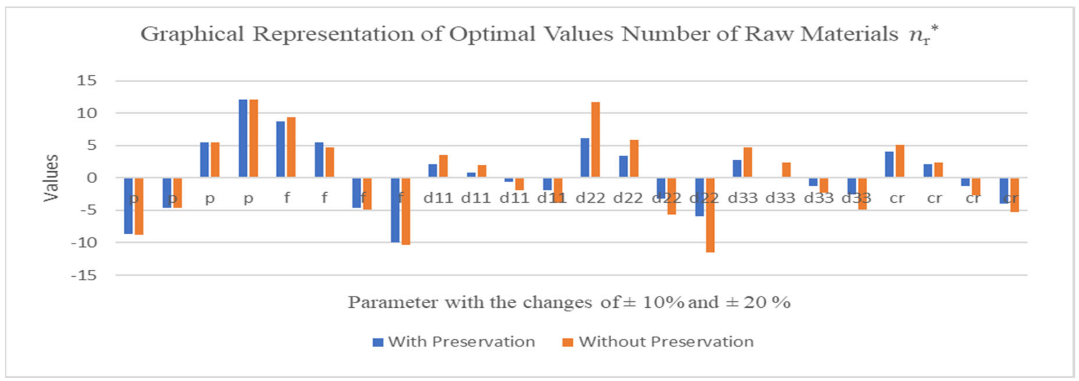
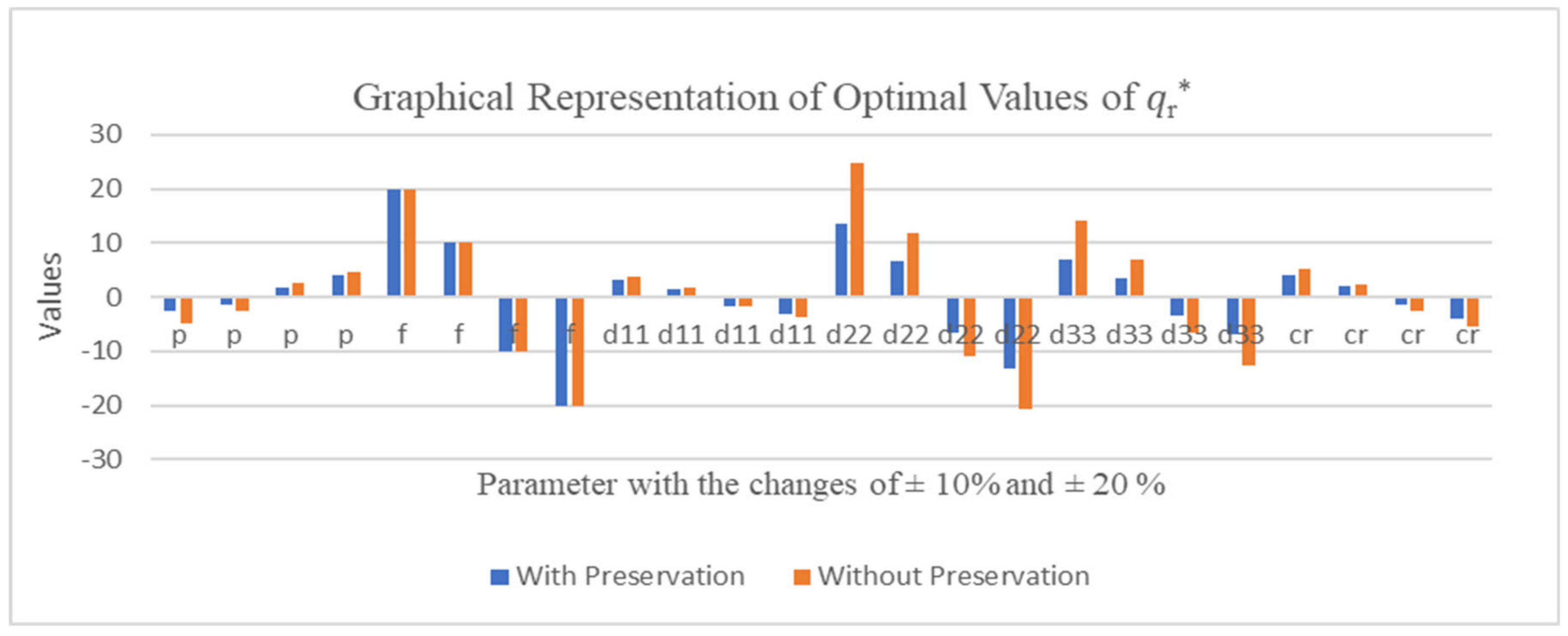
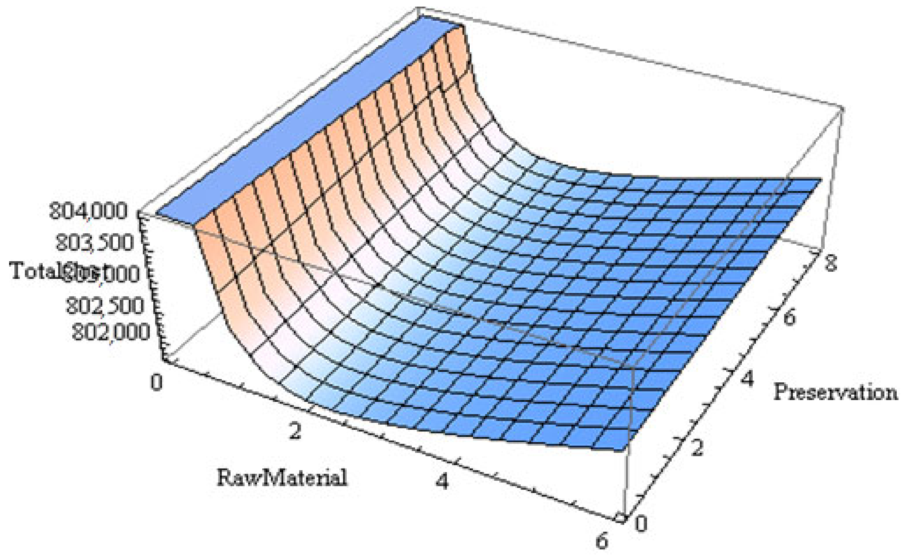
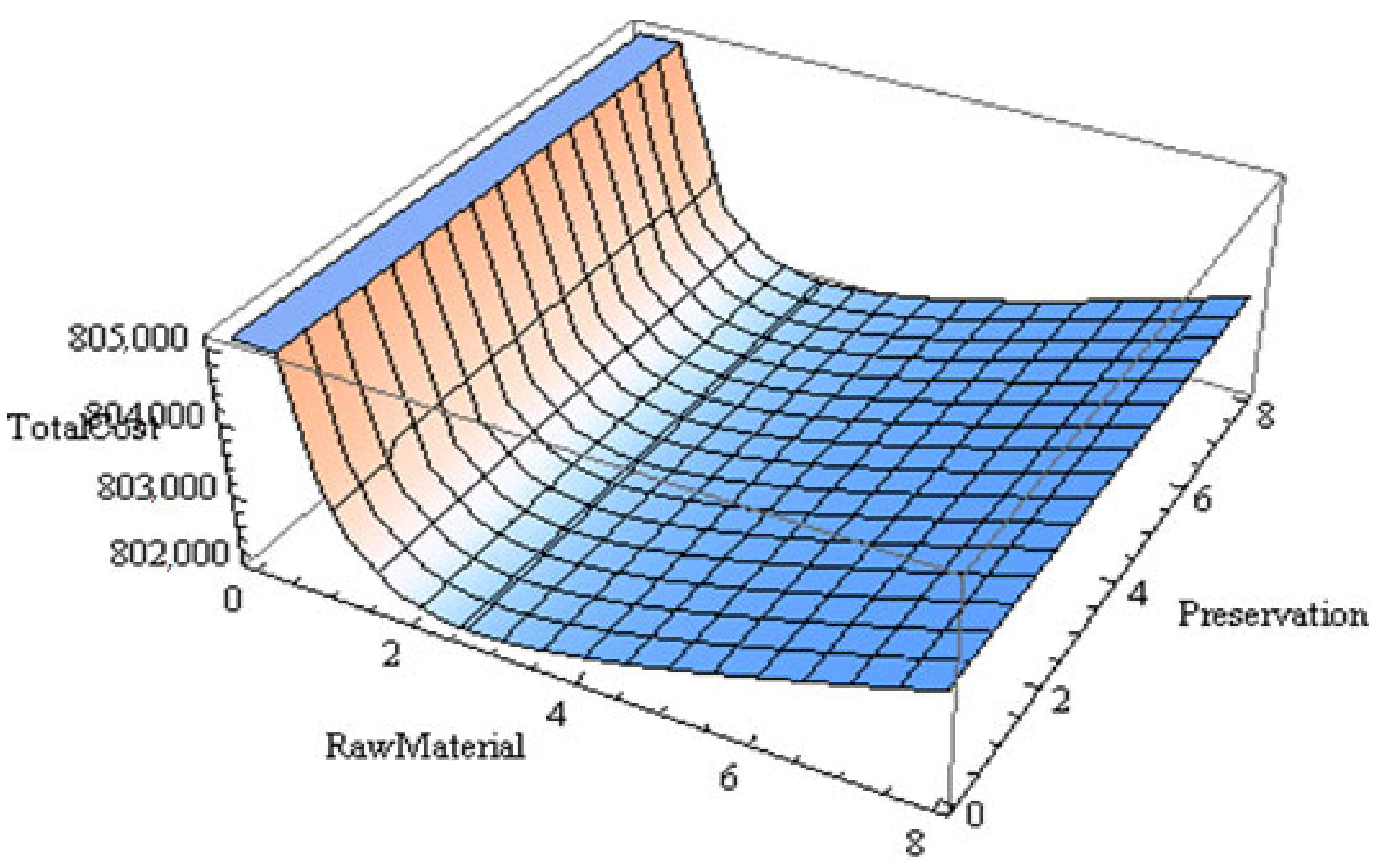
6.2. Graphical Analysis

The graphical illustration of the optimum overall cost with respect to the number of deliveries of raw material with and without preservation technology that is the convexity of the $T{C}^{*}$ with respect to $n_r^{*}$ has been shown in Figure 11 and Figure 12, respectively. Convexity of the optimal cost, preservation technology and raw material 3-dimensional figure has been shown in Figure 13 and Figure 14.

7. Managerial Implication

In business, success in logistics translated to increased efficiencies, lower costs, higher production rates, better inventory control, more innovative use of warehouse space, increased customer and supplier satisfaction and an improved customer experience. These findings are a systematic approach to sourcing, storing and selling inventory—raw materials (components) and finished goods (products). In business, the right stock, at the proper levels, in the right place, at the right time, with the fair cost and price are of paramount values. The proposed model incorporates some realistic features associated with inventories, such as electronic components, fashionable clothes, domestic goods, fruits, fish, etc. Therefore, the managerial implications from the numerical results of our proposed model will be helpful for the retailers doing business on the aforementioned components. In business, success reasonably translated to increased efficiencies, lower costs, higher production rates, better inventory control, more innovative use of warehouse space, increased customer and supplier satisfaction and an improved customer experience.

8. Conclusions

Worldwide markets offer sell openings and posture production the executive’s challenges for makers of deteriorating things. Grasping the advantage of the distinction in planning the selling period of the deteriorating things at various markets offers a unique chance to work on the benefit of a deteriorating producer. This paper investigates the limited recharging stock models of a solitary item with defective production measures. The possibility is higher for the producer to sell the items in various periods and geological areas in various business sectors around the planet with deals season to accomplish higher benefits. It is a one-of-a-kind chance to improve the productivity of breaking down things by abusing the distinction in planning the selling period of the decaying things at various business sectors. The model is proficient for the business in which holding cost relies on time. The sensitivity investigation is checked regarding the different boundaries of the framework. It can be seen that the arrangement of the model is very steady. In this paper, a strategy is recommended for discovering the ideal creation and inventory plan for producers of breaking down things by utilizing conservation innovation first; then, the outcome is examined with and without protection innovation. Here, the producer produces in one area and sells in various business sectors that have distinctive selling seasons. It has been shown that the strategy assists with limited expenses and the most incredible benefits. They obtained results to show the legitimacy and soundness of the model. Finally, this paper considers a multiple market demand which plays an important practical role and is a significant part of inventory control and a powerful tool to improve sales and financial return in an industry. These research findings are a systematic approach to sourcing, storing and selling inventory—raw materials (components) and finished goods (products). In business terms, the right stock, at the right levels, in the right place, at the right time, and fair cost and price are inevitable.

Future analysts can conduct research about multi-thing, retail swelling rate, perishability, or discount markdown. One can also consider a multi-echelon supply chain model with setting up cost reduction. Furthermore, last but not least, one can stretch out the proposed model to various genuine based loose conditions, such as stochastic climate, fuzzy climate, delicate climate, harsh climate, etc. A supply chain model with service level constraints and strategies under uncertainty, involvement of controllable lead time and variable demand for an intelligent manufacturing system under a supply chain management.

References

1. Mishra, V.K.; Sahab, S.L. A deteriorating inventory model for time dependent demand and holding cost with partial backlogging. Int. J. Manag. Sci. Eng. Manag. 2011, 6, 267–271. [Google Scholar] [CrossRef]
2. Khara, B.; Dey, J.K.; Mondal, S.K. An inventory model under development cost-dependent imperfect production and reliability-dependent demand. J. Manag. Anal. 2017, 4, 258–275. [Google Scholar] [CrossRef]
3. Benkherouf, L.; Skouri, K.; Konstantaras, I. Optimal batch production with rework process for products with time-varying demand over finite planning horizon. In Operations Research, Engineering and Cyber Security; Springer: Cham, Switzerland, 2017; Volume 113, pp. 57–68. [Google Scholar]
4. Demirag, O.C.; Kumar, S.; Rao, K.M. A note on inventory policies for products with residual-life-dependent demand. Appl. Math. Model. 2017, 43, 647–658. [Google Scholar] [CrossRef]
5. Bera, A.K.; Jana, D.K. Multi-item imperfect production inventory model in Bi-fuzzy environments. Opsearch 2017, 54, 260–282. [Google Scholar] [CrossRef]
6. Mahata, G.C. A production-inventory model with imperfect production process and partial backlogging under learning considerations in fuzzy random environments. J. Intell. Manuf. 2017, 28, 883–897. [Google Scholar] [CrossRef]
7. Nobil, A.H.; Cárdenas-Barrón, L.E. Some observations to: Lot sizing with non-zero setup times for rework. Int. J. Appl. Comput. Math. 2017, 3, 1511–1517. [Google Scholar] [CrossRef]
8. Dizbin, N.M.; Tan, B. Optimal control of production-inventory systems with correlated demand inter-arrival and processing times. Int. J. Prod. Econ. 2020, 228, 107692. [Google Scholar]
9. Maihami, R.; Kamalabadi, I.N. Joint pricing and inventory control for non- instantaneous deteriorating items with partial backlogging and time and price dependent demand. Int. J. Prod. Econ. 2012, 136, 116–122. [Google Scholar] [CrossRef]
10. Ghoreishi, M.; Weber, G.W.; Mirzazadeh, A. An inventory model for non-instantaneous deteriorating items with partial backlogging, permissible delay in payments, inflation-and selling price-dependent demand and customer returns. Ann. Oper. Res. 2015, 226, 221–238. [Google Scholar] [CrossRef]
11. Yang, C.T.; Ouyang, L.Y.; Wu, K.S.; Yen, H.F. An optimal replenishment policy for deteriorating items with stock-dependent demand and relaxed terminal conditions under limited storage space. Cent. Eur. J. Oper. Res. 2011, 19, 139–153. [Google Scholar] [CrossRef]
12. Banerjee, S.; Agrawal, S. Inventory model for deteriorating items with freshness and price dependent demand, optimal discounting and ordering policies. Appl. Math. Model. 2017, 52, 53–64. [Google Scholar] [CrossRef]
13. Hsu, P.H.; Wee, H.M.; Tang, H.M. Preservation technology investment for deteriorating inventory. Int. J. Prod. Econ. 2010, 124, 388–394. [Google Scholar] [CrossRef]
14. He, Y.; Huang, H.H. Optimizing inventory and pricing policy for deteriorating seasonal products with preservation technology investment. J. Ind. Eng. 2013, 2013, 793568. [Google Scholar]
15. Dye, C.Y. The effect of preservation technology investment on a no instantaneous deteriorating inventory model. Omega 2013, 41, 872–880. [Google Scholar] [CrossRef]
16. Mishra, U.; Crdenas-Barrn, L.E.; Tiwari, S.; Shaikh, A.A.; Trevio-Garza, G. An inventory model under price and stock dependent demand for controllable deterioration rate with shortages and preservation technology investment. Ann. Oper. Res. 2017, 252, 165–190. [Google Scholar]
17. Shen, Y.; Shen, K.; Yang, C. A production inventory model for deteriorating items with collaborative preservation technology investment under carbon tax. Sustainability 2019, 11, 5027. [Google Scholar] [CrossRef] [Green Version]
18. Bardhan, S.; Pal, H.; Giri, B.C. Optimal replenishment policy and preservation technology investment for a non-instantaneous deteriorating item with stock-dependent demand. Oper. Res. 2017, 19, 247–368. [Google Scholar] [CrossRef]
19. Mashud, A.H.M.; Roy, D.; Daryanto, Y.; Chakrabortty, R.K.; Tseng, M.L. A sustainable inventory model with controllable carbon emissions, deterioration and advance payments. J. Clean. Prod. 2021, 296, 126608. [Google Scholar] [CrossRef]
20. Taleizadeh, A.A. A constrained integrated imperfect manufacturing-inventory system with preventive maintenance and partial backordering. Ann. Oper. Res. 2018, 261, 303–337. [Google Scholar] [CrossRef]
21. Sarkar, M.; Lee, Y.H. Optimum pricing strategy for complementary products with reservation price in a supply chain model. J. Ind. Manag. Optim. 2017, 13, 1553. [Google Scholar] [CrossRef] [Green Version]
22. Alfares, H.K.; Ghaithan, A.M. Inventory and pricing model with price-dependent demand, time-varying holding cost, and quantity discounts. Comput. Ind. Eng. 2016, 94, 170–177. [Google Scholar] [CrossRef]
23. Sarkar, B.; Sana, S.S.; Chaudhuri, K. An imperfect production process for time varying demand with inflation and time value of money—an EMQ model. Expert Syst. Appl. 2011, 38, 13543–13548. [Google Scholar] [CrossRef]
24. Pervin, M.; Roy, S.K.; Weber, G.W. An integrated inventory model with variable holding cost under two levels of trade-credit policy. Numer. Algebra Control Optim. 2018, 8, 169. [Google Scholar] [CrossRef] [Green Version]
25. Cárdenas-Barrón, L.E.; Mandal, B.; Sicilia, J.; San-José, L.A.; Abdul-Jalbar, B. Optimizing price, order quantity, and backordering level using a nonlinear holding cost and a power demand pattern. Comput. Oper. Res. 2021, 133, 105339. [Google Scholar] [CrossRef]
26. Palanivel, M.; Suganya, M. Partial backlogging inventory model with price and stock level dependent demand, time varying holding cost and quantity discounts. J. Manag. Anal. 2021, 8, 1–28. [Google Scholar] [CrossRef]
27. Mishra, V.K. An inventory model of instantaneous deteriorating items with controllable deterioration rate for time dependent demand and holding cost. J. Ind. Eng. Manag. 2013, 6, 495–509. [Google Scholar] [CrossRef]
28. Nasr, W.W.; Salameh, M.K.; Moussawi-Haidar, L. Integrating the economic production model with deteriorating raw material over multi production cycles. Int. J. Prod. Res. 2014, 52, 2477–2489. [Google Scholar] [CrossRef]
29. Bhunia, A.; Shaikh, A. A deterministic inventory model for deteriorating items with selling price dependent demand and three-parameter Weibull distributed deterioration. Int. J. Ind. Eng. Comput. 2014, 5, 497–510. [Google Scholar] [CrossRef] [Green Version]
30. Duari, N.K.; Chakraborti, T. An order level EOQ model for deteriorating items in a single warehouse system with price depended demand and shortages. Am. J. Eng. Res. 2014, 3, 11–16. [Google Scholar]
31. Nobil, A.H.; Sedigh, A.H.A.; Cárdenas-Barrón, L.E. A multiproduct single machine economic production quantity (EPQ) inventory model with discrete delivery order, joint production policy and budget constraints. Ann. Oper. Res. 2020, 286, 265–301. [Google Scholar] [CrossRef]
32. AL-Khazraji, H.; Cole, C.; Guo, W. Optimization and simulation of dynamic performance of production–inventory systems with multivariable controls. Mathematics 2021, 9, 568. [Google Scholar] [CrossRef]
33. Uthayakumar, R.; Tharani, S. An economic production model for deteriorating items and time dependent demand with rework and multiple production setups. J. Ind. Eng. Int. 2017, 13, 499–512. [Google Scholar] [CrossRef] [Green Version]
34. He, Y.; Wang, S.Y.; Lai, K.K. An optimal production-inventory model for deteriorating items with multiple-market demand. Eur. J. Oper. Res. 2010, 203, 593–600. [Google Scholar] [CrossRef]
35. Singh, S.R.; Malik, A.K.; Gupta, S.K. Two warehouses inventory model with partial back ordering and multi-variate demand under inflation. Int. J. Oper. Res. Optim. 2011, 2, 371–384. [Google Scholar]
36. Sajadifar, S.M.; Hashempour, M. An optimal production-inventory model for deteriorating items with multiple-market demand under backlogging. In Proceedings of the 2012 International Conference on Industrial Engineering and Operations Management, Istanbul, Turkey, 3–6 July 2012; pp. 1735–1743. [Google Scholar]
37. Malik, A.K.; Shrma, A. An inventory model for deteriorating items with multi-variate demand and partial backlogging under inflation. Int. J. Math. Sci. 2011, 3, 315–321. [Google Scholar]
38. He, Y.; Wang, S. Analysis of production-inventory system for deteriorating items with demand disruption. Int. J. Prod. Res. 2012, 50, 4580–4592. [Google Scholar] [CrossRef]
39. Karimi, M.; Sadjadi, S.J. Optimization of a multi-Item inventory model for deteriorating items with capacity constraint using dynamic programming. J. Ind. Manag. Optim. 2020, 18, 1–16. [Google Scholar] [CrossRef]
40. Singhal, S.; Singh, S.R. Supply chain system for time and quality dependent decaying items with multiple market demand and volume flexibility. Int. J. Oper. Res. 2018, 31, 245–261. [Google Scholar] [CrossRef]
41. Chakraborty, D.; Jana, D.K.; Roy, T.K. Multi-warehouse partial backlogging inventory system with inflation for non-instantaneous deteriorating multi-item under imprecise environment. Soft Comput. 2020, 24, 14471–14490. [Google Scholar] [CrossRef]
42. Pal, B.; Sana, S.S.; Chaudhuri, K. A three-layer multi-item production–inventory model for multiple suppliers and retailers. Econ. Model. 2012, 29, 2704–2710. [Google Scholar] [CrossRef]
43. Khurana, D. Two warehouse inventory model for deteriorating items with time dependent demand under inflation. Int. J. Comput. Appl. 2015, 114, 34–38. [Google Scholar] [CrossRef]
44. Tiwari, S.; Jaggi, C.K.; Bhunia, A.K.; Shaikh, A.A.; Goh, M. Two-warehouse inventory model for non-instantaneous deteriorating items with stock-dependent demand and inflation using particle swarm optimization. Ann. Oper. Res. 2017, 254, 401–423. [Google Scholar] [CrossRef]
45. Jauhari, A.W.; Pujawan, N.I. Joint economic lot size (JELS) model for single-vendor single-buyer with variable production rate and partial backorder. Int. J. Oper. Res. 2014, 20, 91–108. [Google Scholar] [CrossRef]
46. Thinakaran, N.; Jayaprakas, J.; Elanchezhian, C. Survey on inventory model of EOQ & EPQ with partial backorder problems. Mater. Today: Proc. 2019, 16, 629–635. [Google Scholar]
47. Taleizadeh, A.A.; Cárdenas-Barrón, E.L.; Mohammadi, B. A deterministic multi product single machine EPQ model with backordering, scraped products, rework and interruption in manufacturing process. Int. J. Prod. Econ. 2014, 150, 9–21. [Google Scholar] [CrossRef]
48. Singh, D. Production inventory model of deteriorating items with holding cost, stock, and selling price with backlog. Int. J. Math. Oper. Res. 2019, 14, 290–305. [Google Scholar] [CrossRef]
49. Chatterji, D.; Gothi, B.U. EOQ model for deteriorating items under two and three parameter Weibull distribution and constant IHC with partially backlogged shortages. Int. J. Sci. Eng. Technol. Res. (IJSETR) 2015, 4, 3582–3594. [Google Scholar]
50. Palanivel, M.; Uthayakumar, R. An EPQ model for deteriorating items with variable production cost, time dependent holding cost and partial backlogging under inflation. Opsearch 2015, 52, 1–17. [Google Scholar] [CrossRef]
51. Cárdenas-Barrón, E.L. The derivation of EOQ/EPQ inventory models with two backorders costs using analytic geometry and algebra. Appl. Math. Model. 2011, 35, 2394–2407. [Google Scholar] [CrossRef] [Green Version]
52. Taleizadeh, A.; Hazarkhani, B.; Moon, I. Joint pricing and inventory decisions with carbon emission considerations, partial backordering and planned discounts. Ann. Oper. Res. 2020, 290, 95–113. [Google Scholar] [CrossRef]
53. Prasad, K.; Mukherjee, B. Optimal inventory model under stock and time dependent demand for time varying deterioration rate with shortages. Ann. Oper. Res. 2016, 243, 323–334. [Google Scholar] [CrossRef]
54. De, S.K.; Sana, S.S. An EOQ model with backlogging. Int. J. Manag. Sci. Eng. Manag. 2016, 11, 143–154. [Google Scholar]
55. San-José, L.A.; Sicilia, J.; González-De-la-Rosa, M.; Febles-Acosta, J. Optimal inventory policy under power demand pattern and partial backlogging. Appl. Math. Model. 2017, 46, 618–630. [Google Scholar] [CrossRef]
56. Sarkar, T.; Ghosh, S.K.; Chaudhuri, K.S. An optimal inventory replenishment policy for a deteriorating item with time-quadratic demand and time-dependent partial backlogging with shortages in all cycles. Appl. Math. Comput. 2012, 218, 9147–9155. [Google Scholar] [CrossRef]
57. Choudhury, K.D.; Karmakar, B.; Das, M.; Datta, T.K. An inventory model for deteriorating items with stock-dependent demand, time-varying holding cost and shortages. Opsearch 2015, 52, 55–74. [Google Scholar] [CrossRef]
58. Wuu Wu, J.; Chuan Lee, W. An EOQ inventory model for items with Weibull deterioration, shortages and time varying demand. J. Inf. Optim. Sci. 2013, 24, 103–122. [Google Scholar]
59. Sarkar, B.; Majumder, A.; Sarkar, M.; Kim, N.; Ullah, M. Effects of variable production rate on quality of products in a single-vendor multi-buyer supply chain management. Int. J. Adv. Manuf. Technol. 2018, 99, 567–581. [Google Scholar] [CrossRef]
60. Dey, B.K.; Sarkar, B.; Pareek, S. A two-echelon supply chain management with setup time and cost reduction, quality improvement and variable production rate. Mathematics 2019, 7, 328. [Google Scholar] [CrossRef] [Green Version]
61. Sett, B.K.; Dey, B.K.; Sarkar, B. The effect of O2O retail service quality in supply chain management. Mathematics 2020, 8, 1743. [Google Scholar] [CrossRef]
62. Dey, B.K.; Bhuniya, S.; Sarkar, B. Involvement of controllable lead time and variable demand for a smart manufacturing system under a supply chain management. Expert Syst. Appl. 2021, 184, 115464. [Google Scholar] [CrossRef]
Figure 1. Graphical represent of the problem.
Sustainability 13 12601 g001
Figure 2. Graphical representation of the production inventory model without shortages.
Sustainability 13 12601 g002
Figure 3. Graphical representation of raw materials of inventory system.
Sustainability 13 12601 g003
Figure 4. Graphical representation of final production inventory level with shortage under backlogging.
Sustainability 13 12601 g004
Figure 5. Changes the values of the given parameter with respect to   ξ * .
Sustainability 13 12601 g005
Figure 6. Changes the values of the given parameter with respect to   T 1 * .
Sustainability 13 12601 g006
Figure 7. Changes the values of the given parameter with respect to nr*.
Sustainability 13 12601 g007
Figure 8. Changes the values of the given parameter with respect to q r * .
Sustainability 13 12601 g008
Figure 9. Changes the values of the given parameter with respect to T C * (Without shortage).
Sustainability 13 12601 g009
Figure 10. Changes the values of the given parameter with respect to T C * (With shortage).
Sustainability 13 12601 g010
Figure 11. With preservation technology.
Sustainability 13 12601 g011
Figure 12. Without preservation technology.
Sustainability 13 12601 g012
Figure 13. The portrayed are raw material ( n r * ), preservation ( ξ * ) and the total cost ( T C * ), along the x-axis, the y-axis and the z-axis, respectively.
Sustainability 13 12601 g013
Figure 14. Graphical representation to show the convexity of the total cost is described. The portrayed are raw material ( n r * ), preservation ( ξ * ) and the total cost ( T C * ), along the x-axis, the y-axis and the z-axis, respectively.
Sustainability 13 12601 g014