Model of Color Parameters Variation and Correction in Relation to “Time-View” Image Acquisition Effects in Wheat Crop


1
Soil Science and Plant Nutrition, Banat University of Agricultural Sciences and Veterinary Medicine “King Michael I of Romania”, Timisoara 300645, Romania
2
Remote Sensing and GIS, Banat University of Agricultural Sciences and Veterinary Medicine “King Michael I of Romania”, Timisoara 300645, Romania
3
Mathematic and Statistics, Banat University of Agricultural Sciences and Veterinary Medicine “King Michael I of Romania”, Timisoara 300645, Romania
*
Author to whom correspondence should be addressed.
Sustainability 2020, 12(6), 2470; https://doi.org/10.3390/su12062470
Submission received: 5 February 2020
/
Revised: 10 March 2020
/
Accepted: 19 March 2020
/
Published: 21 March 2020
(This article belongs to the Section Environmental Sustainability and Applications)
Abstract
:Many images of agricultural crops are made at different times of the day, images with different spectral information about the same crop in relation to conditions when the picture was taken. A set of 30 digital images of a wheat crop in the BBCH 3-Stem elongation code 32–33 stage was captured between 9 am and 14 (UTC+3), in the 0°–180° variation range of the image acquisition angle on the E-W axis (cardinal directions). A high variation of the spectral data given by the combination of the hour (h) and angle (a) at which the images were captured was found. The interdependence relationship between the analyzed parameters (r, g, and b), and the time (t) and the angle (a) of image acquisition was assessed with the linear correlation coefficient. By calculating the roots of the mathematical expressions of the correlation coefficients dependence on the angles (a) or times of day (t), the optimal angle and time were determined as a combination of the two variables for capturing images and obtaining optimal ro, go, bo values. The correction coefficients of the normalized r, g, and b values obtained out of the optimal field were determined. To this end, the multiplication of the r(a,t), g(a,t), and b(a,t) values with the ρa,t, γa,t, and βa,t correction coefficients was suggested to reach the optimal values for sustainable decisions.
1. Introduction
The imaging-based techniques for earth’s crust, plant cover, and crop investigation have developed and diversified dramatically. As a result, image analysis has come to rely on satellite imagery [1,2,3], aerial images (utility aircraft or drones) [4,5], or terrestrial images taken with commercial cameras or cameras mounted on agricultural machinery and equipment [6,7,8].
To assess agricultural crop vegetation and yield relative to the environmental and technological factors such as fertilizer dosage, irrigation, phytosanitary condition etc., classical methods can be employed, but they are expensive and slow as opposed to imagery techniques [9,10]. As an alternative solution, methods based on imagery analysis have been promoted increasingly in practice and research activities [11,12,13,14].
The new investigation methods bring more precision to agricultural practice, as they provide real-time information for adequate crop management corresponding to the nutritional status, the flowering structure, the phytosanitary condition, the reaction to various stress factors (hydric, thermal etc.,), the yield estimation and even the interventions required to compensate different deficiency in crops [15,16,17,18,19].
Operational environmental factors such as the camera height, the angle to the horizon, and the distance to the target object refer mainly to the image geometry and can be established as being constant, to have a uniform distribution of the absorption and radiation properties of the target area. There are also other environmental factors in the image acquisition area [20,21] such as: a different architecture of wheat plants, the degree of coverage and the green conditions of leaves, the intensity, spectral composition and luminosity of the photographed object. These factors are influenced especially by weather conditions. Consequently, the use of working methods that provide color stability may reduce the degree of uncertainty that characterizes the assessment of the physiological parameters of plants whose study is based on their color.
The purpose of this study was to determine the optimal angle for image capture so that the r, g, and b color indices may not be affected (or be affected in the smallest possible degree) by the moment chosen for taking the photographs. At the same time, the study intended to determine what the best time is to take photos on crops so that the r, g, and b color indices may not be affected by the image capture angle. The determination of these parameters and their simultaneous practical application may lead to a decrease in the variation of the value of the studied color indices. The study proposed a model and correction coefficients of the normalized r, g, and b values obtained for images acquired at other angles or times, then those suggested as optimal in this study.
2. Materials and Methods
2.1. Location and Experimental Conditions
The study was conducted in the Educational and Experimental Station of the Banat University of Agricultural Sciences and Veterinary Medicine “King Michael I of Romania” (BUASVM) from Timisoara, Romania. The experimental field was located in Plot A 363 and had the following geographic coordinates: N 45°28′ and 30.9″, E 21°7′9.8″. The climate characteristics—an average multiannual rainfall of 603.3 mm and an average temperature of 10.9 °C—are specific to the temperate continental climate with Mediterranean influences. In autumn, the field was fertilized with phosphorous, potassium and one-third of the nitrogen dose (mixed granular fertilizer). The remaining nitrogen was applied as urea next spring, before the stem elongation stage, the general fertilization being P100K100N100 (P100 represents 100 kg·ha−1 active substance (a.c.) phosphorus (P), and similarly for kallium (K) and for nitrogen (N). This level was considered optimal for the climatic and agro-chemical conditions of the area, for a 6 t ha−1 yield.
2.2. Biological Material and Crop Status
The biological material was Triticum aestivum L. Alex cultivar, a genotype with great yield potential and very good quality indices that is grown not only in Romania, but also in other countries. The main growth stage 3—Stem elongation scale for cereals was selected for image acquisition. Detailing phenological aspects, converted in crop development codes, according to BBCH-scale [22,23], the wheat plants were in the growth stage 3—Stem elongation, more exactly in 32 (Node 2 at least 2 cm above node 1) and 33 stage (Node 3 at least 2 cm above node 2). This growth stage was chosen because it is considered to be very predictable when fertilized with nitrogen and in relation to the further development of the wheat crop [24,25].
2.3. Taking Photos and Digital Images Analyzation
The digital images were taken in a visible spectrum with a commercial digital camera with proper technical parameters: NIKON D300, 12 MP resolution, DX format. The images were acquired from a uniform wheat crop in a sunny day (24 April 2013), during 9.00 to 14.00 (noted in the article as “t”) and at different camera angles (noted “a”, expressed sexagesimal degrees) on the E-W axis (0°, 45°, 90°, 135°, and 180°) (Figure 1). Throughout this paper, the time format used is hh.mm.ss, according to Time Zone UTC+3.00.
The constant parameters were the following: the camera height (1.5 m), the 45° angle to the horizontal line, the 24-mm lens and the 52.4° lens angle, full frame (Figure 2). Each acquired image covered equal crop areas of about 3 m2, with a mean density of about 1550 wheat plants. The images were recorded hourly from 9.00 to 14.00, from E to W, at 0°, 45°, 90°, 135°, and 180°, resulting in a set of 30 images in jpg format (Figure 3).
The image resolution was 4288 x 2848 pixels, 300 dpi, 24 bits for Adobe RGB. The average image size was 9.54 MB. The images were processed with ImageJ software [26] to obtain the mean values of the R, G, B parameters (R—spectral values in red channel; G—spectral values in green channel; B—spectral values in blue channel). Based on the values R, G, B normalized values have been calculated, noted as r, g, respectively b (r = R/(R + G + B), g = G/(R + G + B), b = B/(R + G + B)).
Based on them, the normalized r,g,b values [27] and the specific indices intensity—INT [28], Equation (1), normalized difference index—NDI [29] Equation (2), and dark green color index—DGCI [30] Equation (3) were calculated. In Equation (3) H—hue; S—saturation; B—brightness in HSB color system, have been used for calculating DGCI according to [30], and for B in HSB system the symbol BHSB has been used in order to avoid confusion with B in RGB system.
2.4. Experimental Data Analysis
The interdependence relationship between the analyzed parameters (r, g, and b) and the hour (t) and angle (a) of image acquisition was assessed with the linear correlation coefficient. A high correlation indicates a great dependence between the parameters and the determination factors, i.e., a high contribution of the two variables to the values of the indices, while a low correlation indicates the independence from the parameters.
The values of the coefficients of correlation between the r, g, and b series and the moments (t) the images were acquired (9 a.m., 10 a.m., 11 a.m., 12 a.m., 1 p.m., 2 p.m.) in relation to the angles at which the photos were taken (0°, 45°, 90°, 135°, 180°) were calculated; the coefficients of correlation between the r, g, and b series and the angles (a) at which the photos were taken at different moments (t) were calculated as well.
A high correlation coefficient (absolute value, namely close to −1 or 1) will show that a slight change of the moment chosen to take the photo in relation to the angle (a) or a change of the angle in relation to time indicates a change in the r, g, and b color indices. At the same time, a correlation coefficient close to zero will indicate that even a significant change of the time chosen to take the photo in relation to the angle, or vice versa, does not imply a change in the r, g, and b color indices. Next the mathematical expressions of the correlation coefficients dependence on angles (a) or times (t) were determined. By calculating the roots of these expressions, we were able to determine the optimal image acquisition angle so that the color indices might not be affected by time, as well as the optimal time in relation to the angle.
The calculation of the correlation coefficients, their graphic representations, the determination of the regression equations for several variable functions and other calculations were done with Microsoft Excel. The polynomial regression equations were determined with PAST 3 [31]. For the graphic representations of the constant level curves and the algebraic calculus the Wolfram Alpha software was used.
3. Results
3.1. Subheadings Image Acquisition
The combination of the two variables against which the images were acquired, namely the time (6 different hours) and the angle (5 angles on the E-W axis), generated a set of 30 digital images of the same plant cover represented by the autumn wheat crop, Alex cultivar. From the image analysis performed with the ImageJ 1.48r software the spectral data specific to the r, g, and b bands were retrieved. Based on these data, the normalized rgb values and the INT (intensity), NDI (normalized difference index), and DGCI (dark green color index) indices used to characterize the plant cover were calculated. The results are given in Table 1.
The r, g, and b values series is highly heterogeneous. The variation coefficients obtained by relating the standard deviation to the value mean were 5.5% for r, 6.4% for g, and 22.9% for b. The same was found for the INT, NDI, and DGCI parameters that also had a high variation coefficient in absolute value (15.4%, 19.4%, and 18.15%). This implies a wide variety of color hues (Figure 4), which recovers the colors of the images acquired in the field based on the r, g, and b value set given in Table 1.
3.2. Normalized r,g,b—Time (t) Correlation at Different Angle (a)
Based on the data in Table 1, the data in Table 2 have been calculated, which provides the coefficients of linear correlation between the r and t series, then g and t series, respectively b and t series, for each shooting angle in part (a) separately.
Based on the data in Table 2, the expressions of Equations (4)–(6) describing the correlation coefficient variation with the angle were obtained, under very high correlation conditions. These were written as and their polynomial expressions were calculated with Past3. The graphical representations of the Equations (4) to (6) are represented on Figure 5.
The roots of Equations (7)–(9) simplified as (determined with Wolfram Alpha) and marked ar, ag, and ab respectively will indicate the angle at which the correlation coefficient is zero, i.e., the optimal angle at which photos can be taken so that the color indices may not be affected by the image acquisition time. From these roots, only that which is close to angle (a) variation range, i.e., from 0° to 90°, will be chosen.
3.3. Normalized r,g,b—Angle (a) Correlation at Different Time (t)
The values of the coefficients of correlation between the series of r, g, and b values and the angle series (0°, 45°, 90°, 135°, 180°) were calculated similarly. In Table 3, the values of the correlation coefficients are given separately, on each row, to correspond to the image acquisition time.
The graphic representations of the equations describing the variation of the correlation coefficients with time marked hr(t), hg(t), hb(t) (Figure 6), have the analytical expressions given in Equations (10)–(12). For all three equations, the value of the correlation coefficient was very high (0.99)
The roots of the equations that are close to the variation range of the studied time range (9–14, UTC+3), determined with the Wolfram Alpha software, will indicate the time when the correlation coefficient is zero, i.e., the optimal time at which the photos can be taken so that the color indices may not be affected by the acquisition angle. The following solutions (16) to Equations (13), (14) and (15) were obtained:
As an observation, the mathematical expressions of the correlation coefficients were third-degree polynomials, and the only roots of interest were those close to the studied variation range both for the time and the angle of image acquisition.
The r(a,t) dependence relationships in Equation (17), g(a,t) in Equation (18) and b(a,t) in Equation (19), between the normalized r, g, and b coefficients, the angle (a) value and the time (t) at which they were calculated were determined:
The regression Equation (17) has a high correlation coefficient value (0.99), and the p values of each separate coefficient of the regression equation reach a maximum of p = 0.0104. For Equation (18), R2 = 0.99, and p is smaller than p = 0.0255, respectively for Equation (19) (0.99) and p is smaller than p = 0.0300. In all situations, this provides statistical certainty at level (the calculations were done with Excel/Data analysis/Regression).
The optimal r value was determined for the optimal angle (a) values in Equations (7)–(9), and for the time (t) values in Equation (16), and the optimal values for the r, g, b in relation to time and angle are presented in Equations (20)–(22):
3.4. Corrections Model
Subsequently, the problem was raised to determine the correction coefficients of the normalized r, g, and b values obtained for images acquired at other angles or times than those suggested as optimal in this study. To this end, the multiplication of the r(a,t), g(a,t) și b(a,t) values with the ρa,t, γa,t, and βa,t correction coefficients was suggested to reach the optimal values, as shown in Equations (23)–(25):
As an observation, are two-dimensional matrices that include the correction coefficients for r, g, and b, and their values were calculated and are given in Table 4, Table 5 and Table 6.
Given that real difficulties may occur in practice when determining the exact angle at which images were acquired—for instance, some trips cannot be planned at previously established hours for time reasons (Figure 7) provides graphic representations of the constant level curves that indicate possible combinations between other angle and time values and may lead to r, g, and b values closer to the optimal values. The graphic representations were done with the Wolfram Alpha software. On these images, the suggested optimal values (relative to the stability of the image acquisition process) are marked with a dot. It is easy to notice that their positioning makes them different from the maximum values of the functions. Additionally, the areas around the optimal values to which r, g, and b tend if the angle or time is changed are colored differently. The spectral data-based characterization of vegetation stages, health status or various physiological parameters of plants in agricultural crops or biomass yield has become a common practice in agricultural technologies. Besides the classical satellite-based approach in crop characterization, a series of agricultural machinery have already been equipped with photo/video cameras or high-resolution sensors that capture real-time images of crops [32].
4. Discussion
The acquisition of crop images has often proved inconsistent and the color data are influenced by certain particularities. Studies dealing with such issues have recommended techniques and working models to improve color stability significantly [33,34]. Reflectance is high due to vegetation uniformity [35] and if the soil is not completely covered in vegetation, reflectance may have a dramatic influence on the RGB parameters and may reduce the quality of the correlation between the indices calculated based on spectral or RGB parameters and the nutritional status [24].
The multiple correlations between the plant color, chlorophyll content, and the health or nutritional status of plants show that imaging methods are adequate for agricultural applications [24,25,36]. Chlorophyll absorbs light and transfers light energy to trigger photochemical reactions. It is one of the photo chemically active compounds in photosynthesis. Chlorophyll quantity and quality are reflected in plant color; therefore sunlight is absorbed or reflected in different degrees. Crop reflectance depends on many environmental factors including incident illumination, the physiological status of the crop, and the calibration of the photographic reaction in fields in accordance with the reactions in the measured areas [16,20,21,37,38], and provides the basis for determining plant nutrition deficiencies. In this study, while the crop was uniform, we discovered a certain variation of the color parameters (r, b, and g) relative to the time and angle of image acquisition, following the change of the solar illumination angle in relation to the studied area. This case may occur in real practice, when images are acquired by agricultural machinery in real time, while wheat or other crops are being tended. Reflectance as influenced by the solar illumination angle in some crops has been dealt with in other studies as well [39,40,41,42]. The spectacular evolution of high-definition image acquisition methods in mobile telephony and the development of new mobile applications for the management of various agricultural aspects have created a new niche with great potential for improving applied agricultural research [14].
The literature of on this topic provides different approaches of image acquisition: spectral techniques and photographic techniques. The former (multispectral, hyper spectral imaging) records images to analyze crops and the plant cover with radio spectrographs especially in the visible and infrared range (400–1000 nm). The spectral indices calculated with the reflectance data have proved to have an indirect connection with the nutritional status and the biomass yield of many crops (maize, wheat, soy, cotton, and broccoli), the quantification of the degree of vegetation coverage, and agricultural efficiency [37,43,44,45,46,47,48,49,50,51]. Such techniques usually acquire images from considerable heights using satellites or aircraft and are especially helpful to monitor and analyze larger areas. This spectacular combination of space and imaging technology requires the involvement of governments or multinationals operating in larger farms.
The current technological progress of cameras combined with data storage, processing, and transmission technologies turn cameras and digital capture systems into valuable tools of sustainable, precise agriculture not only in the present, but also in the future. The technical specifications of photographic cameras, such as the optical and electronic parameters and image processing software quality, have reached a high performance level. Remarkable progress has been made in this field. Inexpensive commercial cameras with superior technical characteristics are now available [52]. The photographic techniques applied in visible or infrared ranges with high-definition cameras use RGB or other derived parameters at minimum cost affordable for small and medium-sized farms [13,24,27,52,53,54,55]. Digital camera captures images as a matrix of individual pixels that record the red (R), green (G), and blue (B) intensities. The RGB channels are subsequently used either to classify images or, if combined in spectral indices, to correlate with the relevant parameters [52,56].
RGB or spectral image analysis has been applied in agriculture not only for nutritional status assessment, but also for other purposes like weed identification [57], crop and weed mapping [58], crop and weed discrimination [59], quantification of turf grass color [30], quantitative analysis of specially variable physiological process across leaf surface [60], quantification of damage caused by various crop pathogens [61], seed color test for identification of qualitative and commercial seed traits [62], and research in the in vitro tissue cultures [56].
In both cases, the real research field is dynamic, the methodologies may overlap (multi-spectral photographic cameras), and as a general feature, all results are published faster than before and become available to agricultural practice and farmers [14].
Although wheat crops, given their economic importance, were among the first to be investigated by remote sensing and image analysis, applied research has employed mostly spectral methods and techniques [15,20,35,63,64,65,66], while the photographic techniques in the visible range are not so commonly used and developed afterwards, with the evolution of the photographic digital cameras [24,25,55].
This study has attempted to add to the known approaches the analysis of the influence of certain operational environmental parameters (time and angle) on the RGB image parameters (normalized r, g and b) resulting from the study of a wheat crop based on digital terrestrial images.
5. Conclusions
Following image acquisition in the field, it has been noticed that the time and the angle at which images were captured are the factors leading to different r, g, and b values. Their series were characterized by high variation coefficients (5, 6, 22% respectively), therefore the hues resulted after acquiring the image of the same subject differed. This could lead to false interpretations in the assessment of the physiological status of plants and crop wheat characterization based on color parameters data. As a result, a correction is required of the variation values of the two factors.
The determined constant level curves can provide important information about the selected angle-time combinations. If it is impossible to fall within ranges close to the optimal values, the optimal r, b, and g values can be estimated based on the multiplication with the calculated correction coefficients.
This study may describe only a particular case from among the numerous concrete situations provided by the combination of crop/directions/angle and solar light, but it can represent a calculation model for other particular cases in agricultural holdings.
Author Contributions
Conceptualization, F.S. and C.A.P.; methodology, F.S.; software, M.V.H.; validation, F.S., C.A.P. and M.V.H.; formal analysis, C.R.; investigation, F.S.; resources, M.V.H.; data curation, C.R.; writing—original draft preparation, F.S.; writing—review and editing, F.S. and C.R.; visualization, M.V.H. and C.A.P. All authors have read and agreed to the published version of the manuscript.
Funding
The research is supported by the project “Ensuring excellence in the activity of RDI within USAMVBT” code 35PFE, submitted in the competition Program 1—Development of the national system of research—evelopment, Subprogram 1.2—Institutional performance, Institutional development projects—Development projects of excellence in RDI.
Acknowledgments
The authors thank the staff of the Didactic and Experimental Station of the Banat University of Agricultural Sciences and Veterinary Medicine “King Michael I of Romania” from Timisoara, Romania to facilitate this research. The authors thank the GEOMATICS RESEARCH LABORATORY, BUASMV “King Michael I of Romania” from Timisoara, for the facility of the software use for this research.
Conflicts of Interest
The authors declare no conflict of interest.
References
- Rogan, J.; Franklin, J.; Roberts, D.A. A comparison of methods for monitoring multitemporal vegetation change using Thematic Mapper imagery. Remote Sens. Environ. 2002, 80, 143–156. [Google Scholar] [CrossRef]
- Xie, Y.; Sha, Z.; Yu, M. Remote sensing imagery in vegetation mapping: A review. J. Plant Ecol. 2008, 1, 9–23. [Google Scholar] [CrossRef]
- Panda, S.S.; Hoogenboom, G.; Paz, J.O. Remote sensing and geospatial technological applications for site-specific management of fruit and nut crops: A review. Remote Sens. 2010, 2, 1973–1997. [Google Scholar] [CrossRef] [Green Version]
- Cousins, S.A.O. Analysis of land-cover transitions based on 17th and 18th century cadastral maps and aerial photographs. Landsc. Ecol. 2001, 16, 41–54. [Google Scholar] [CrossRef]
- Lehmann, J.R.K.; Nieberding, F.; Prinz, T.; Knoth, C. Analysis of unmanned aerial system-based CIR images in forestry—A new perspective to monitor pest infestation levels. Forests 2015, 6, 594–612. [Google Scholar] [CrossRef] [Green Version]
- Torii, T. Research in autonomous agriculture vehicles in Japan. Comput. Electron. Agric. 2000, 25, 133–153. [Google Scholar] [CrossRef]
- Slaughter, D.C.; Giles, D.K.; Downey, D. Autonomous robotic weed control systems: A review. Comput. Electron. Agric. 2008, 61, 63–78. [Google Scholar] [CrossRef]
- Emmi, L.; Gonzales-de-Soto, M.; Pajares, G.; Gonzales-de-Santos, P. New trends in robotics for agriculture: Integration and assessment of a real fleet of robots. Sci. World J. 2014, 2014, 404059. [Google Scholar] [CrossRef] [Green Version]
- Van der Werf, H.M.G.; Petit, J. Evaluation of the environmental impact of agriculture at the farm level: A comparison and analysis of 12 indicator-based methods. Agric. Ecosyst. Environ. 2002, 93, 131–145. [Google Scholar] [CrossRef]
- Muñoz-Huerta, R.F.; Guevara-Gonzalez, R.G.; Contreras-Medina, L.M.; Torres-Pacheco, I.; Prado-Olivarez, J.; Ocampo-Velazquez, R.V. A review of methods for sensing the nitrogen status in plants: Advantages, disadvantages and recent advances. Sensors 2013, 13, 10823–10843. [Google Scholar] [CrossRef]
- Fiella, I.; Serrano, L.; Serra, J.; Penuelas, J. Evaluating wheat nitrogen status with canopy reflectance indices and discriminant analysis. Crop Sci. 1995, 35, 1400–1405. [Google Scholar] [CrossRef]
- Doraiswamy, P.C.; Moulin, S.; Cook, P.W.; Stern, A. Crop yield assessment from remote sensing. Photogramm. Eng. Remote Sens. 2003, 69, 665–674. [Google Scholar] [CrossRef]
- Yuzhu, H.; Xiaomei, W.; Song, S. Nitrogen determination in pepper (Capsicum frutescens L.) plants by color image analysis (RGB). Afr. J. Biotechnol. 2011, 10, 17737–17741. [Google Scholar]
- Delgado, J.A.; Kowalski, K.; Tebbe, C. The first Nitrogen Index app for mobile devices: Using portable technology for smart agricultural management. Comput. Electron. Agric. 2013, 91, 121–123. [Google Scholar] [CrossRef]
- Amundson, R.L.; Koehler, F.E. Utilization of DRIS for diagnosis of nutrient deficiencies in winter wheat. Agron. J. 1987, 79, 472–476. [Google Scholar] [CrossRef]
- Carter, G.A. Responses of leaf spectral reflectance to plant stress. Am. J. Bot. 1993, 80, 239–243. [Google Scholar] [CrossRef]
- Manjunath, K.R.; Potbar, M.B. Large area operational wheat yield model development and validation based on spectral and meteorological data. Int. J. Remote Sens. 2002, 23, 3023–3038. [Google Scholar] [CrossRef]
- Merzlyak, M.N.; Gitelson, A.A.; Chivkunova, O.B.; Solovchenko, A.E.; Pogosyan, S.I. Application of reflectance spectroscopy for analysis of higher plant pigments. Russ. J. Plant Physiol. 2003, 50, 704–710. [Google Scholar] [CrossRef]
- Gitelson, A.A.; Chivkunova, O.B.; Merzlyak, M.N. Nondestructive estimation of anthocyanins and chlorophylls in anthocyanic leaves. Am. J. Bot. 2009, 96, 1861–1868. [Google Scholar] [CrossRef]
- Wright, D.L.; Rasmussen, V.P.; Ramsey, R.D.; Baker, D.J. Canopy reflectance estimation of wheat nitrogen content for grain protein management. GISCI Remote Sens. 2004, 41, 287–300. [Google Scholar] [CrossRef]
- De Souza, E.G.; Scharf, P.C.; Sudduth, K.A. Sun position and cloud effects on reflectance and vegetation indices of corn. Agron. J. 2010, 102, 734–744. [Google Scholar] [CrossRef] [Green Version]
- Witzenberger, A.; Hack, H.; van den Boom, T. Erläuterungen zum BBCH-Dezimal-Code für die Entwicklungsstadien des Getreides—Mit Abbildungen. Gesunde Pflanz. 1989, 41, 384–388. [Google Scholar]
- Lancashire, P.D.; Bleiholder, H.; Langeluddecke, P.; Stauss, R.; van den Boom, T.; Weber, E.; Witzen-Berger, A. A uniform decimal code for growth stages of crops and weeds. Ann. Appl. Biol. 1991, 119, 561–601. [Google Scholar] [CrossRef]
- Jia, L.; Chen, X.; Zhang, F.; Buerkert, A.; Römheld, V. Use of digital camera to assess nitrogen status oe winter wheat in the Northern China Plain. J. Plant Nutr. 2004, 27, 441–450. [Google Scholar] [CrossRef]
- Kakran, A.; Mahajan, R. Monitoring growth of wheat crop using digital image processing. Int. J. Comput. Appl. 2012, 50, 18–22. [Google Scholar] [CrossRef]
- Rasband, W.S. ImageJ; U.S. National Institutes of Health: Bethesda, MD, USA, 1997–2018. [Google Scholar]
- Lee, K.-J.; Lee, B.-W. Estimation of rice growth and nitrogen nutrition status using color digital camera image analysis. Eur. J. Agron. 2013, 48, 57–65. [Google Scholar] [CrossRef]
- Ahmad, I.S.; Reid, J.F. Evaluation of colour representations for maize images. J. Agric. Eng. Res. 1996, 63, 185–196. [Google Scholar] [CrossRef]
- Mao, W.; Wang, Y.; Wang, Y. Real-time detection of between—Row weeds using machine vision. In Proceedings of the 2003 ASAE Annual Meeting. American Society of Agricultural and Biological Engineers, Las Vegas, NV, USA, 27–30 July 2003. [Google Scholar]
- Karcher, D.E.; Richardson, M.D. Quantifying turfgrass color using digital image analysis. Crop Sci. 2003, 43, 943–951. [Google Scholar] [CrossRef]
- Hammer, Ø.; Harper, D.A.T.; Ryan, P.D. PAST: Paleontological statistics software package for education and data analysis. Palaeontol. Electron. 2001, 4, 1–9. [Google Scholar]
- Thessler, S.; Kooistra, L.; Teye, F.; Huitu, H.; Bregt, A.K. Geosensors to support crop production: Current applications and user requirements. Sensors 2011, 11, 6656–6684. [Google Scholar] [CrossRef] [Green Version]
- Tendero, Y.; Landeau, S.; Gilles, J. Non-uniformity correction of infrared images by midway equalization. Image Process. Line 2012, 2, 134–146. [Google Scholar] [CrossRef] [Green Version]
- Li, L.; Zhang, Q.; Huang, D. A review of imaging techniques for plant phenotyping. Sensors 2014, 14, 20078–20111. [Google Scholar] [CrossRef]
- Jackson, R.D.; Pinter, P.J.; Idso, S.B.; Reginato, R.J. Wheat spectral reflectance: Interactions between crop configuration, sun elevation, and azimuth angle. Appl. Opt. 1979, 18, 3730–3733. [Google Scholar] [CrossRef]
- Graeff, S.; Claupein, W. A novel approach revealing information on wheat (Triticum aestivum L.) nitrogen status by leaf reflectance measurements. Pflanzenbauwissenschaften 2006, 10, 66–74. [Google Scholar]
- Colwell, J.E. Vegetation canopy reflectance. Remote Sens. Environ. 1974, 3, 175–183. [Google Scholar] [CrossRef]
- Xiao, X.; He, L.; Salas, W.; Li, C.; Moore, B.; Zhao, R.; Frolking, S.; Boles, S. Quantitative relationships between field-measured leaf area index and vegetation index derived from VEGETATION images for paddy rice fields. Int. J. Remote Sens. 2002, 23, 3595–3604. [Google Scholar] [CrossRef]
- Kollenkark, J.C.; Vanderbilt, V.C.; Daughtry, C.S.T.; Bauer, M.E. Influence of solar illumination angle on soybean canopy reflectance. Appl. Opt. 1982, 21, 1179–1184. [Google Scholar] [CrossRef]
- Ranson, K.J.; Biehl, L.L.; Bauer, M.E. Variation in spectral response of soybeans with respect to illumination, view and canopy geometry. Int. J. Remote Sens. 1985, 6, 1827–1842. [Google Scholar] [CrossRef]
- Ranson, K.J.; Daughtry, C.S.T.; Biehl, L.I.; Bauer, M.E. Sun-view angle effects on reflectance factors of corn canopies. Remote Sens. Environ. 1985, 18, 147–161. [Google Scholar] [CrossRef]
- Ranson, K.J.; Daughtry, C.S.T.; Biehl, L.L. Sun angle, view angle, and background effects on spectral response of simulated balsam fir canopies. Photogramm. Eng. Remote Sens. 1986, 52, 649–658. [Google Scholar]
- Sumner, E.M. Use of the DRIS system in foliar diagnosis of crops at high yield levels. Commun. Soil Sci. Plant Anal. 1977, 8, 251–268. [Google Scholar] [CrossRef]
- Bouman, B.A.M. Crop modeling and remote sensing for yield prediction. Neth. J. Agric. Sci. 1995, 43, 143–161. [Google Scholar]
- Phillips, S.B.; Keahey, D.A.; Warren, J.G.; Mullins, G.L. Estimating winter wheat tiller density using spectral reflectance sensors for early-spring, variable rate nitrogen applications. Agron. J. 2004, 96, 591–600. [Google Scholar] [CrossRef]
- Jørgensen, R.N.; Hansen, P.M.; Bro, R. Exploratory study of winter wheat reflectance during vegetative growth using three-mode component analysis. Int. J. Remote Sens. 2006, 27, 919–937. [Google Scholar] [CrossRef]
- Graeff, S.; Pfenning, J.; Claupein, W.; Liebig, H.P. Evaluation of image analysis to determine the n-fertilizer demand of broccoli plants (Brassica oleracea convar. botrytis var. italica). Adv. Opt. Technol. 2008, 2008, 359760. [Google Scholar] [CrossRef] [Green Version]
- Shanahan, J.F.; Kitchen, N.R.; Raun, W.R.; Schepers, J.S. Responsive in-season nitrogen management for cereals. Comput. Electron. Agric. 2008, 6, 51–62. [Google Scholar] [CrossRef] [Green Version]
- Stellacci, A.M.; Castrignanò, A.; Diacono, M.; Troccoli, A.; Ciccarese, A.; Armenise, E.; Gallo, A.; De Vita, P.; Lonigro, A.; Mastro, M.A.; et al. Combined approach based on principal component analysis and canonical discriminant analysis for investigating hyperspectral plant response. Ital. J. Agron. 2012, 7, 247–253. [Google Scholar] [CrossRef] [Green Version]
- Herbei, M.V.; Sala, F. Use Landsat image to evaluate vegetation stage in sunflower crops. AgroLife Sci. J. 2015, 4, 79–86. [Google Scholar]
- Herbei, M.; Sala, F. Biomass prediction model in maize based on satellite images. AIP Conf. Proc. 2016, 1738, 1–4. [Google Scholar]
- Lebourgeois, V.; Bégué, A.; Labbé, S.; Mallavan, B.; Prévot, L.; Roux, B. Can commercial digital cameras be used as multispectral sensors? A crop monitoring test. Sensors 2008, 8, 7300–7322. [Google Scholar] [CrossRef]
- Kawashima, S.; Nakatani, M. An algorithm for estimating chlorophyll content in leaves using a video camera. Ann. Bot. 1998, 81, 49–54. [Google Scholar] [CrossRef] [Green Version]
- Golzarian, M.R.; Frick, R.A. Classification of images of wheat, ryegrass and brome grass species at early growth stages using principal component analysis. Plant Methods 2011, 7, 28. [Google Scholar] [CrossRef] [Green Version]
- Guendouz, A.; Guessoum, S.; Maamari, K.; Hafsi, M. Predicting the efficiency of using the RGB (Red, Green and Blue) reflectance for estimating leaf chlorophyll content of Durum wheat (Triticum durum Desf.) genotypes under semi arid conditions. Am. Eurasian J. Sustain. Agric. 2012, 6, 102–106. [Google Scholar]
- Yadav, S.P.; Ibaraki, Y.; Gupta, D.S. Estimation of the chlorophyll content of micropropagated potato plants using RGB based image analysis. Plant Cell Tissue Org. Cult. 2010, 100, 183–188. [Google Scholar] [CrossRef]
- Hemming, J.; Rath, T. Computer-vision based weed identification under field condition using controlled lighting. J Agric. Eng. Res. 2000, 78, 233–243. [Google Scholar] [CrossRef] [Green Version]
- Tillet, N.P.; Hague, T.; Miles, S.J. A field assessment of a potential method for weed and crop mapping geometry. Comput. Electron. Agric. 2001, 32, 229–246. [Google Scholar] [CrossRef]
- Aitkenhead, M.J.; Dalgetty, I.A.; Mullins, C.E.; McDonald, A.J.S.; Strachan, N.J.C. Weed and crop discrimination using image analysis and artificial intelligence methods. Comput. Electron. Agric. 2003, 39, 157–171. [Google Scholar] [CrossRef]
- Aldea, M.; Frank, T.D.; DeLucia, E.H. A method for quantitative analysis for spatially variable physiological processes across leaf surfaces. Photosynth. Res. 2006, 90, 161–172. [Google Scholar] [CrossRef]
- Mirik, M.; Michels, G.J., Jr.; Kassymzhanova-Mirik, S.; Elliott, N.C.; Catana, V.; Jones, D.B.; Bowling, R. Using digital image analysis and spectral reflectance data to quantify damage by greenbug (Hemitera: Aphididae) in winter wheat. Comput. Electron. Agric. 2006, 51, 86–98. [Google Scholar] [CrossRef]
- Dana, W.; Ivo, W. Computer image analysis of seed shape and seed color of flax cultivar description. Comput. Electron. Agric. 2008, 61, 126–135. [Google Scholar] [CrossRef]
- Fernandez-Gallego, J.A.; Kefauver, S.C.; Vatter, T.; Gutiérrez, N.A.; Nieto-Taladriz, M.T.; Araus, J.L. Low-cost assessment of grain yield in durum wheat using RGB images. Eur. J. Agronom. 2019, 105, 146–156. [Google Scholar] [CrossRef]
- Pinter, P.J.; Jackson, R.D.; Idso, S.B.; Reginato, R.J. Diurnal patterns of wheat spectral reflectances. IEEE Trans. Geosc. Remote Sens. 1983, GE-21, 156–163. [Google Scholar] [CrossRef]
- Pinter, P.J.; Jackson, R.D.; Ezra, C.E.; Gausman, H.W. Sun-angle and canopy-architecture effects on the spectral reflectance of six wheat cultivars. Int. J. Remote Sens. 1985, 6, 1813–1825. [Google Scholar] [CrossRef]
- Shibayama, M.; Wiegand, C.L. View azimuth and zenith, and solar angle effects on wheat canopy reflectance. Remote Sens. Environ. 1985, 18, 91–103. [Google Scholar] [CrossRef]
Figure 1.
Position of the camera and time and angle parameters for image acquisition in a wheat crop.
Figure 1.
Position of the camera and time and angle parameters for image acquisition in a wheat crop.
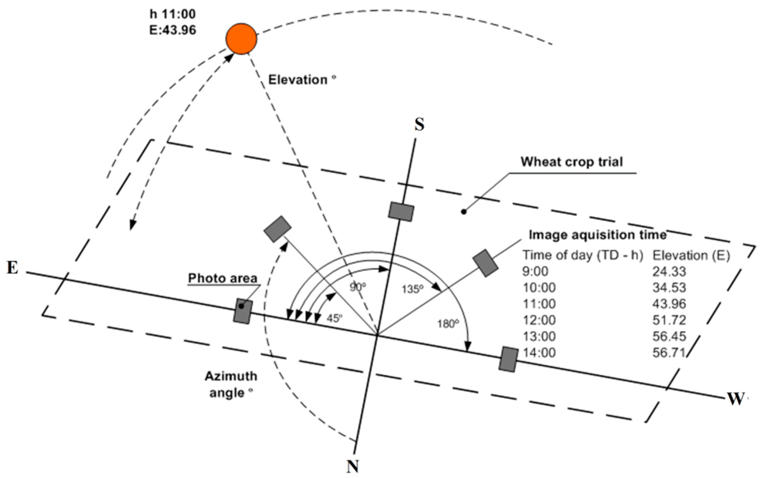
Figure 2.
Photo camera positioning parameters.

Figure 3.
Images of the wheat crop taken at different time and angles.

Figure 4.
Color matrix based on the RGB values in relation to time (t) and angle (a) of image acquisition.
Figure 4.
Color matrix based on the RGB values in relation to time (t) and angle (a) of image acquisition.

Figure 5.
Graphic distribution of the coefficients of correlation between normalized r, g, and b and the image acquisition time (t) at different angles (a).
Figure 5.
Graphic distribution of the coefficients of correlation between normalized r, g, and b and the image acquisition time (t) at different angles (a).

Figure 6.
Graphic distribution of the coefficients of correlation between normalized r, g, and b and the angles (a) of images acquisition at different times of day (t).
Figure 6.
Graphic distribution of the coefficients of correlation between normalized r, g, and b and the angles (a) of images acquisition at different times of day (t).
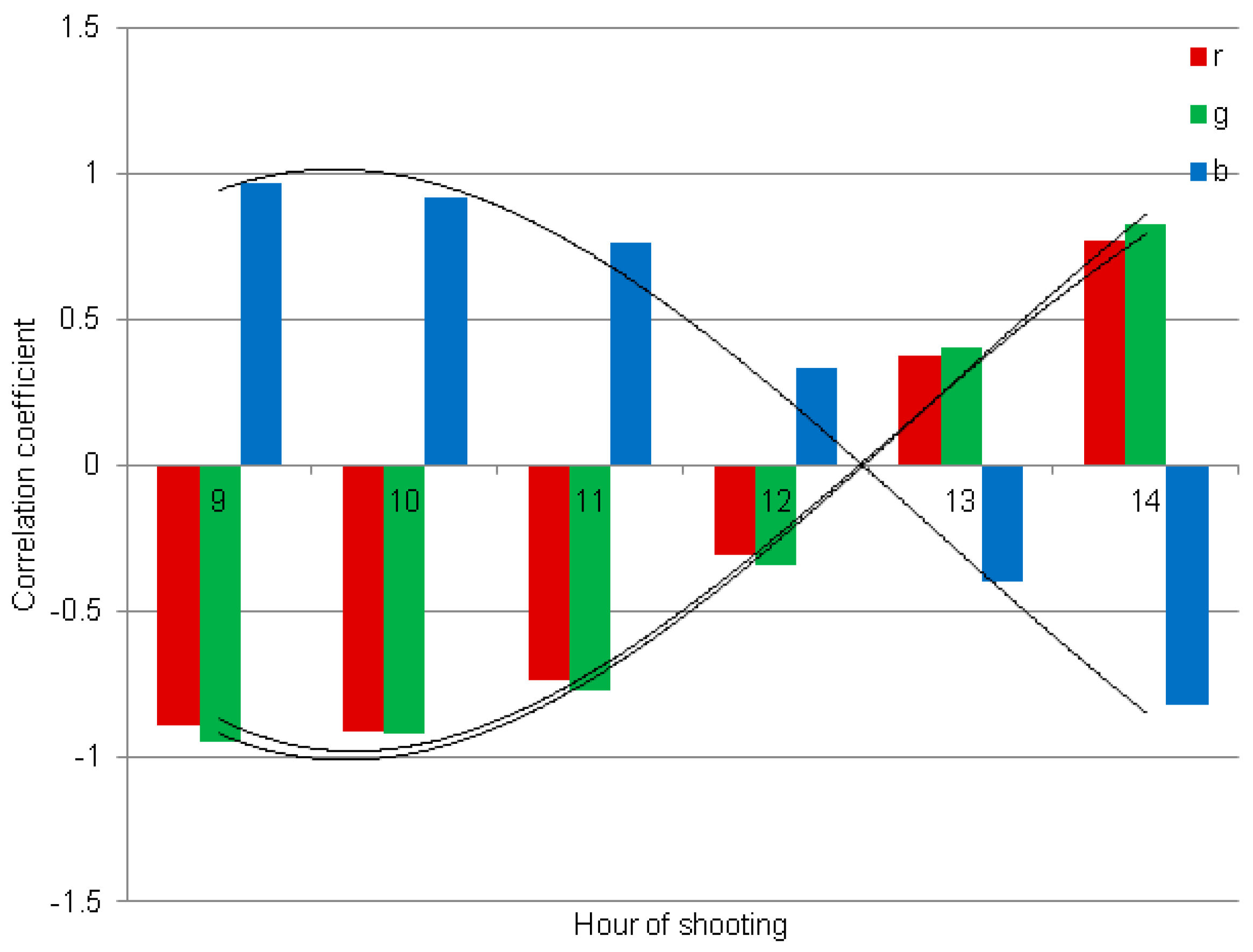
Figure 7.
Graphs of constant level curves of r (a), g (b), and b (c), for the angle and time values (created with Wolfram Alpha).
Figure 7.
Graphs of constant level curves of r (a), g (b), and b (c), for the angle and time values (created with Wolfram Alpha).


Table 1.
Normalized r,g,b and indices values corresponding to the images acquired at different angles and times.
Table 1.
Normalized r,g,b and indices values corresponding to the images acquired at different angles and times.
| Time (GMT+3) (t) | Azimuth | Elevation | Angle (a) | r | g | b | INT | NDI | DGCI |
|---|---|---|---|---|---|---|---|---|---|
| 9 | 96.63 | 24.51 | 0 | 0.330 | 0.530 | 0.139 | 73.570 | −0.229 | 0.439 |
| 45 | 0.341 | 0.517 | 0.143 | 64.567 | −0.203 | 0.452 | |||
| 90 | 0.323 | 0.486 | 0.191 | 72.433 | −0.198 | 0.513 | |||
| 135 | 0.311 | 0.447 | 0.242 | 82.303 | −0.177 | 0.596 | |||
| 180 | 0.293 | 0.455 | 0.253 | 64.137 | −0.214 | 0.676 | |||
| 10 | 108.47 | 34.53 | 0 | 0.369 | 0.486 | 0.146 | 88.147 | −0.136 | 0.383 |
| 45 | 0.378 | 0.499 | 0.123 | 93.887 | −0.136 | 0.339 | |||
| 90 | 0.360 | 0.474 | 0.165 | 102.493 | −0.135 | 0.382 | |||
| 135 | 0.339 | 0.434 | 0.227 | 116.137 | −0.122 | 0.466 | |||
| 180 | 0.331 | 0.410 | 0.259 | 124.887 | −0.105 | 0.521 | |||
| 11 | 122.96 | 43.96 | 0 | 0.350 | 0.471 | 0.179 | 95.430 | −0.146 | 0.422 |
| 45 | 0.369 | 0.498 | 0.132 | 102.140 | −0.147 | 0.340 | |||
| 90 | 0.360 | 0.486 | 0.154 | 103.690 | −0.148 | 0.371 | |||
| 135 | 0.337 | 0.450 | 0.212 | 107.593 | −0.142 | 0.459 | |||
| 180 | 0.325 | 0.415 | 0.259 | 120.507 | −0.120 | 0.536 | |||
| 12 | 141.51 | 51.73 | 0 | 0.341 | 0.452 | 0.208 | 103.833 | −0.138 | 0.459 |
| 45 | 0.358 | 0.487 | 0.155 | 93.317 | −0.152 | 0.391 | |||
| 90 | 0.365 | 0.494 | 0.142 | 100.000 | −0.149 | 0.359 | |||
| 135 | 0.350 | 0.471 | 0.179 | 107.750 | −0.145 | 0.399 | |||
| 180 | 0.332 | 0.432 | 0.237 | 114.517 | −0.130 | 0.490 | |||
| 13 | 165.24 | 56.46 | 0 | 0.329 | 0.429 | 0.243 | 107.740 | −0.130 | 0.521 |
| 45 | 0.344 | 0.465 | 0.191 | 100.110 | −0.149 | 0.437 | |||
| 90 | 0.358 | 0.486 | 0.156 | 102.200 | −0.149 | 0.374 | |||
| 135 | 0.359 | 0.484 | 0.157 | 109.273 | −0.147 | 0.364 | |||
| 180 | 0.337 | 0.450 | 0.213 | 109.933 | −0.142 | 0.452 | |||
| 14 | 191.95 | 56.73 | 0 | 0.333 | 0.415 | 0.252 | 118.900 | −0.109 | 0.510 |
| 45 | 0.340 | 0.447 | 0.213 | 101.363 | −0.134 | 0.472 | |||
| 90 | 0.357 | 0.471 | 0.172 | 101.930 | −0.136 | 0.394 | |||
| 135 | 0.372 | 0.492 | 0.137 | 105.383 | −0.137 | 0.334 | |||
| 180 | 0.354 | 0.469 | 0.176 | 104.350 | −0.138 | 0.391 |
Table 2.
Values of the coefficients of correlation between normalized r, g, and b and time (t) at different angles (a) of image acquisition.
Table 2.
Values of the coefficients of correlation between normalized r, g, and b and time (t) at different angles (a) of image acquisition.
| Angle (a) | r | g | b |
|---|---|---|---|
| 0 | −0.395 | −0.983 | 0.986 |
| 45 | −0.395 | −0.973 | 0.873 |
| 90 | 0.588 | −0.192 | −0.422 |
| 135 | 0.962 | 0.926 | −0.993 |
| 180 | 0.879 | 0.473 | −0.885 |
Table 3.
Values of the coefficients of correlation between normalized r, g, and b and angles (a) of image acquisition at different times of day (t).
Table 3.
Values of the coefficients of correlation between normalized r, g, and b and angles (a) of image acquisition at different times of day (t).
| Time (GMT+2) | r | g | b |
|---|---|---|---|
| 9 | −0.892 | −0.949 | 0.968 |
| 10 | −0.915 | −0.920 | 0.915 |
| 11 | −0.737 | −0.773 | 0.759 |
| 12 | −0.313 | −0.348 | 0.334 |
| 13 | 0.375 | 0.402 | −0.398 |
| 14 | 0.767 | 0.828 | −0.822 |
Table 4.
Matrix of ρ coefficients for r value correction.
| Hour/Angle | 0° | 15° | 30° | 45° | 60° | 75° | 90° |
|---|---|---|---|---|---|---|---|
| 9 | 1.059023 | 1.054631 | 1.053435 | 1.055414 | 1.060604 | 1.069099 | 1.081059 |
| 10 | 1.034768 | 1.026829 | 1.021986 | 1.020152 | 1.021295 | 1.025435 | 1.032645 |
| 11 | 1.028831 | 1.017307 | 1.008937 | 1.003572 | 1.001119 | 1.001534 | 1.004825 |
| 12 | 1.040586 | 1.025066 | 1.012925 | 1.003938 | 0.997946 | 0.994843 | 0.994577 |
| 13 | 1.071283 | 1.050918 | 1.03436 | 1.021286 | 1.011452 | 1.00468 | 1.000851 |
| 14 | 1.124396 | 1.097702 | 1.07554 | 1.057439 | 1.043036 | 1.032052 | 1.024285 |
Table 5.
Matrix of γ coefficients for g value correction.
| Hour/Angle | 0° | 15° | 30° | 45° | 60° | 75° | 90° |
|---|---|---|---|---|---|---|---|
| 9 | 1.005337 | 1.001366 | 1.00109 | 1.004503 | 1.011682 | 1.022789 | 1.038083 |
| 10 | 0.997142 | 0.9887 | 0.98394 | 0.982757 | 0.985126 | 0.991097 | 1.000804 |
| 11 | 1.009517 | 0.996261 | 0.986909 | 0.981253 | 0.979167 | 0.980606 | 0.985601 |
| 12 | 1.044049 | 1.025002 | 1.01037 | 0.999804 | 0.993064 | 0.989997 | 0.990537 |
| 13 | 1.105488 | 1.078756 | 1.057373 | 1.040781 | 1.02857 | 1.020449 | 1.016231 |
| 14 | 1.203548 | 1.165623 | 1.13472 | 1.109916 | 1.09052 | 1.076022 | 1.06606 |
Table 6.
Matrix of β coefficients for b value correction.
| Hour/Angle | 0° | 15° | 30° | 45° | 60° | 75° | 90° |
|---|---|---|---|---|---|---|---|
| 9 | 1.211144 | 1.228411 | 1.219851 | 1.186519 | 1.132312 | 1.06291 | 0.984449 |
| 10 | 1.042227 | 1.083681 | 1.106936 | 1.109476 | 1.091017 | 1.053582 | 1.000974 |
| 11 | 0.907673 | 0.961616 | 1.004588 | 1.032773 | 1.043386 | 1.035318 | 1.009414 |
| 12 | 0.798488 | 0.858024 | 0.912503 | 0.958201 | 0.991399 | 1.009034 | 1.009351 |
| 13 | 0.7085 | 0.769565 | 0.830044 | 0.887002 | 0.936901 | 0.975969 | 1.000788 |
| 14 | 0.633347 | 0.693569 | 0.756407 | 0.819954 | 0.881494 | 0.937547 | 0.984149 |
© 2020 by the authors. Licensee MDPI, Basel, Switzerland. This article is an open access article distributed under the terms and conditions of the Creative Commons Attribution (CC BY) license (http://creativecommons.org/licenses/by/4.0/).
Share and Cite
MDPI and ACS Style
Sala, F.; Popescu, C.A.; Herbei, M.V.; Rujescu, C. Model of Color Parameters Variation and Correction in Relation to “Time-View” Image Acquisition Effects in Wheat Crop. Sustainability 2020, 12, 2470. https://doi.org/10.3390/su12062470
AMA Style
Sala F, Popescu CA, Herbei MV, Rujescu C. Model of Color Parameters Variation and Correction in Relation to “Time-View” Image Acquisition Effects in Wheat Crop. Sustainability. 2020; 12(6):2470. https://doi.org/10.3390/su12062470
Chicago/Turabian StyleSala, Florin, Cosmin Alin Popescu, Mihai Valentin Herbei, and Ciprian Rujescu. 2020. "Model of Color Parameters Variation and Correction in Relation to “Time-View” Image Acquisition Effects in Wheat Crop" Sustainability 12, no. 6: 2470. https://doi.org/10.3390/su12062470
Note that from the first issue of 2016, this journal uses article numbers instead of page numbers. See further details here.