Study on Applicability of Distributed Hydrological Model under Different Terrain Conditions

Abstract
:1. Introduction
2. Materials and Methods
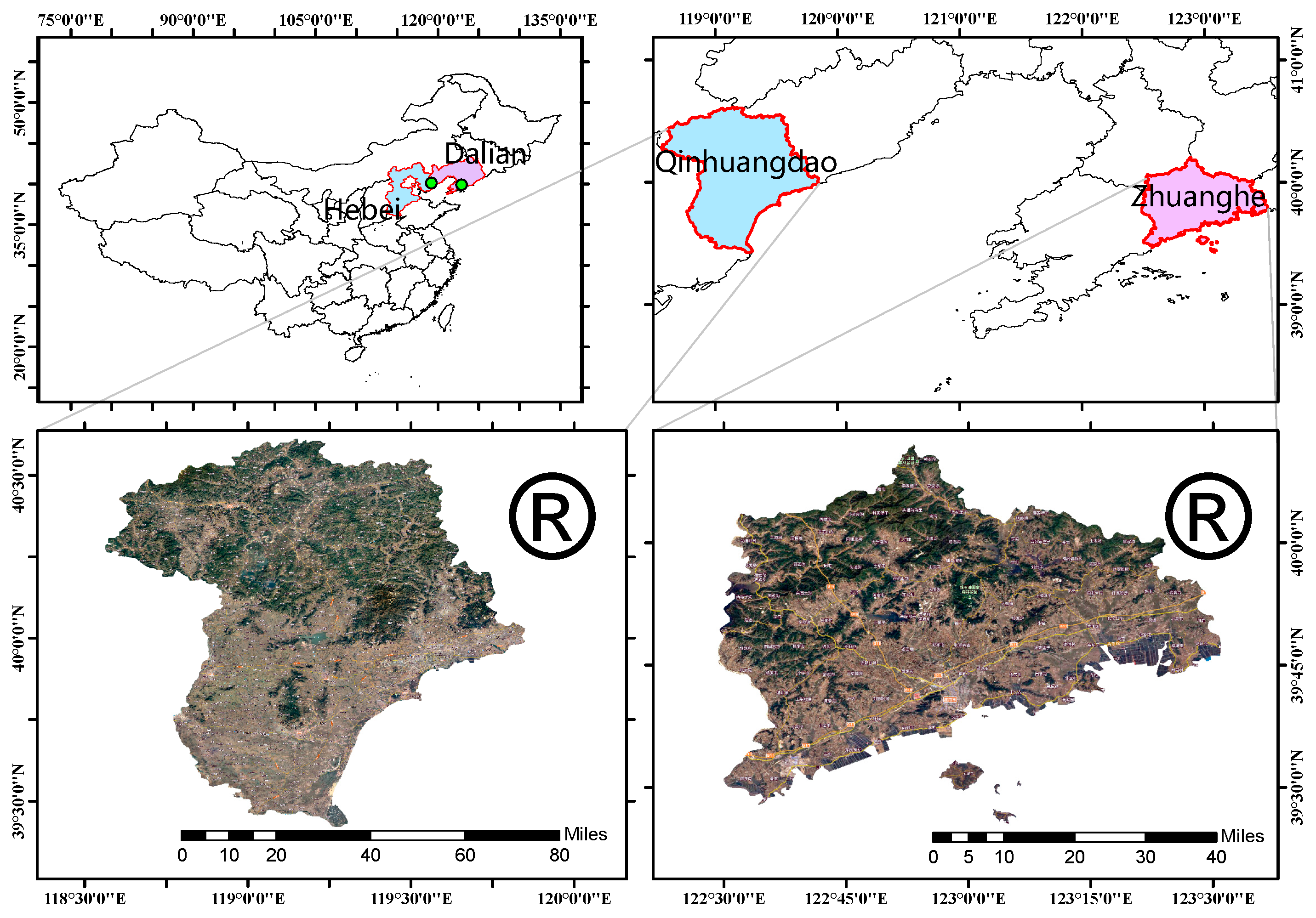
2.1. Study Area
2.2. Database Construction
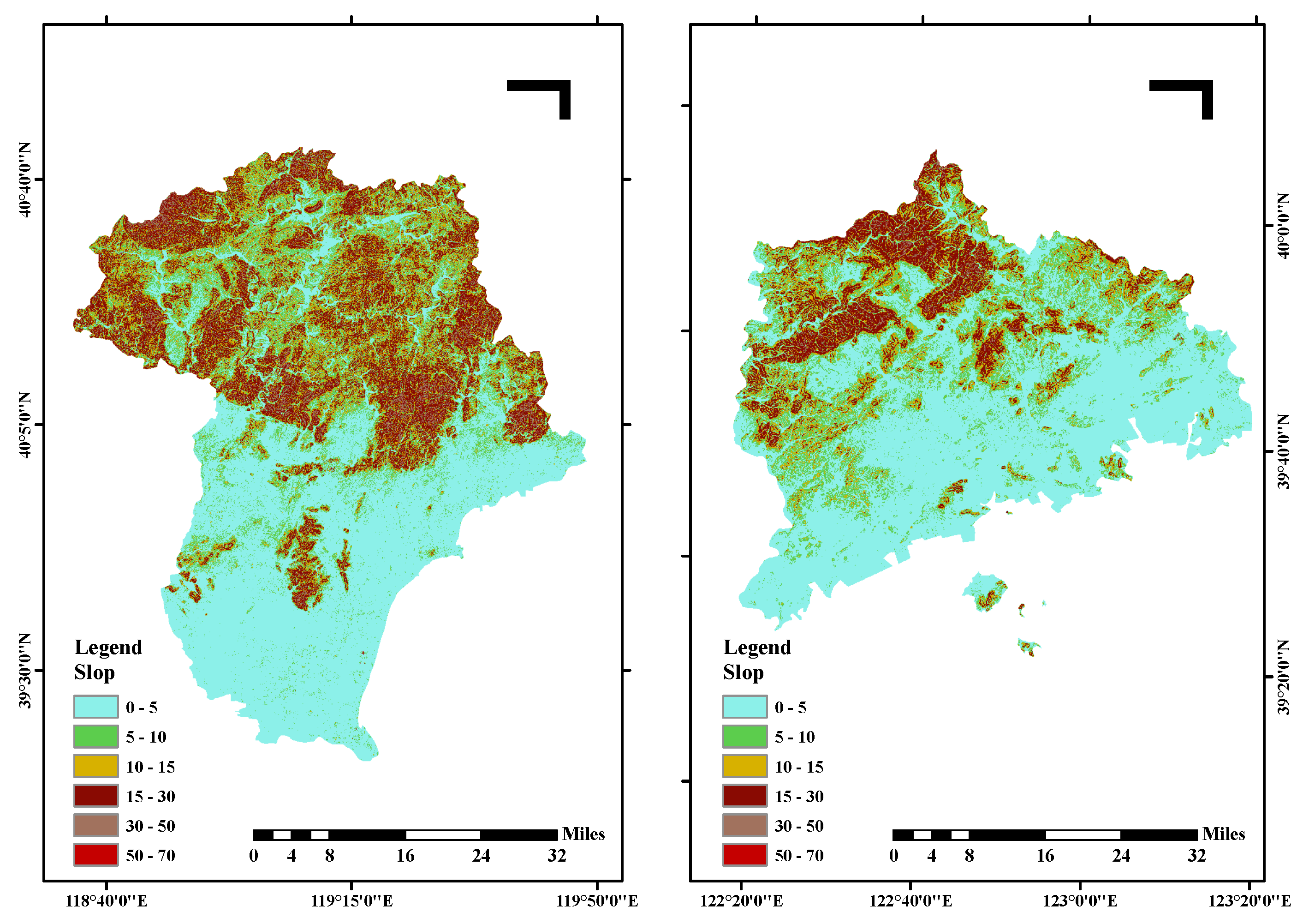
2.2.1. DEM Slope Analysis
2.2.2. Land Use
2.2.3. Soil
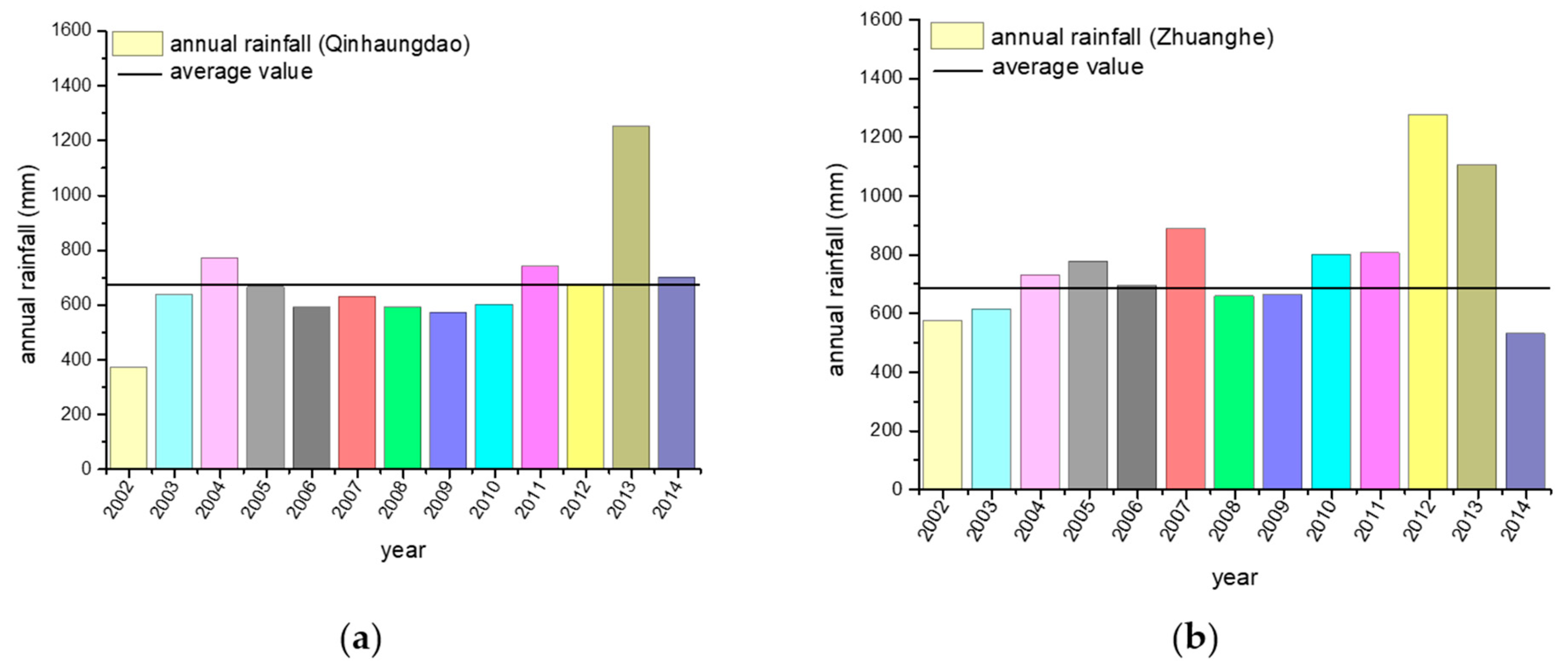
2.2.4. Meteorology
2.3. Modeling Technique Methodology
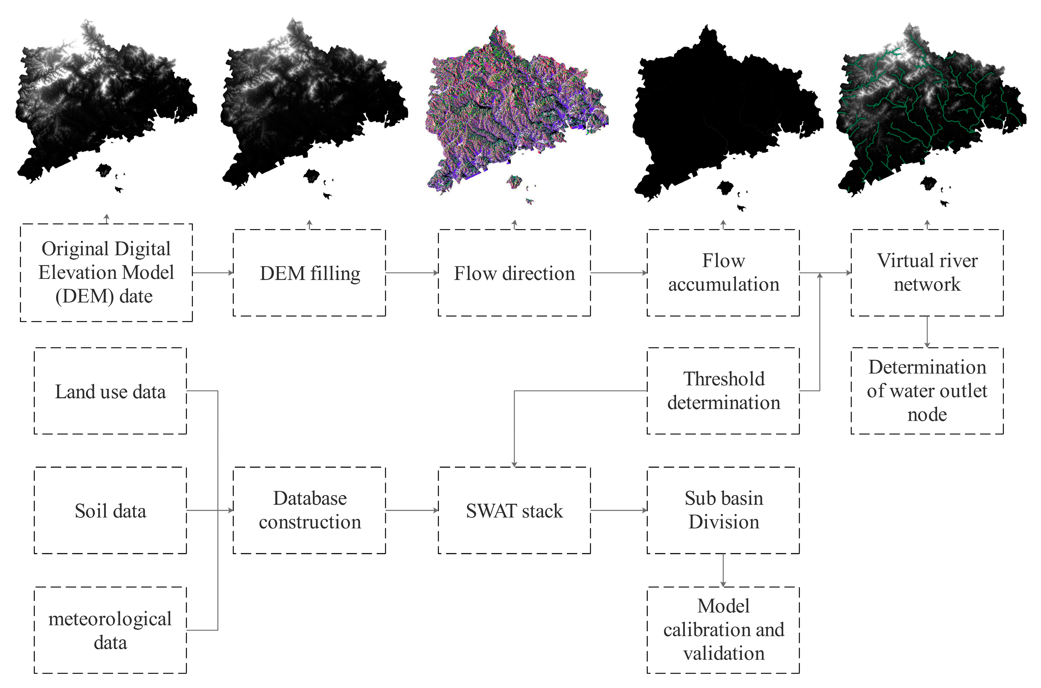
2.3.1. Hydrological Analysis
- Depression-free DEM generation: due to the resolution of the DEM data and the real terrain, there are always some depressions in the image data. To calculate the flow direction correctly, it is necessary to fill the original DEM first to get a non-depression DEM [31]. Extracting water flow direction: this paper used D8 algorithm [32] in GIS to calculate the water flow direction. The algorithm assumed that there are only 8 possible flow directions in a single grid, and the 8 directions are coded with different codes: 1—due east, 2—southeast, 4—due south, 8—southwest, 16—due west, 32—northwest, 64—due north, 128—northeast (Figure 7).The flow direction of a grid cell is defined as the cell with the steepest slope among the 8 grid points adjacent to it. The slope calculation is shown in Equation (1):where is the height of the grid unit, is the height of the adjacent grid unit, and D is the distance between the center points of the two grids. If the two grid cells are adjacent in the horizontal or vertical direction, D is the cell length; if it is in the diagonal direction, D is 2× cell length. According to this principle, the flow direction of all grid points in DEM was calculated one by one to obtain the flow direction raster map.
- 2.
- Cumulative consolidation: assuming that DEM has one unit of water at each grid unit represented by a regular grid, the cumulative amount of confluence at each grid unit can be obtained by calculating the water flow through each grid unit according to the determined flow direction data of the grid unit. Grid units with high confluence accumulation values generally correspond to the rivers, and grid units with cumulative accumulation values of 0 generally correspond to watersheds.
- 3.
- River network extraction: at present, the surface runoff model is mainly used to extract river networks. When the cumulative amount of confluence reaches a certain value, surface runoff will be formed. All the cumulative amount of confluence grid above the critical value will form a potential flow path. A river network is the network composed of these paths. The complex rivers with lines are amended to single rivers, the ring-shaped river networks are amended to dendritic drainage, and the rivers with more complex bends are amended to facilitate subsequent node selection and sub-basin division.
- 4.
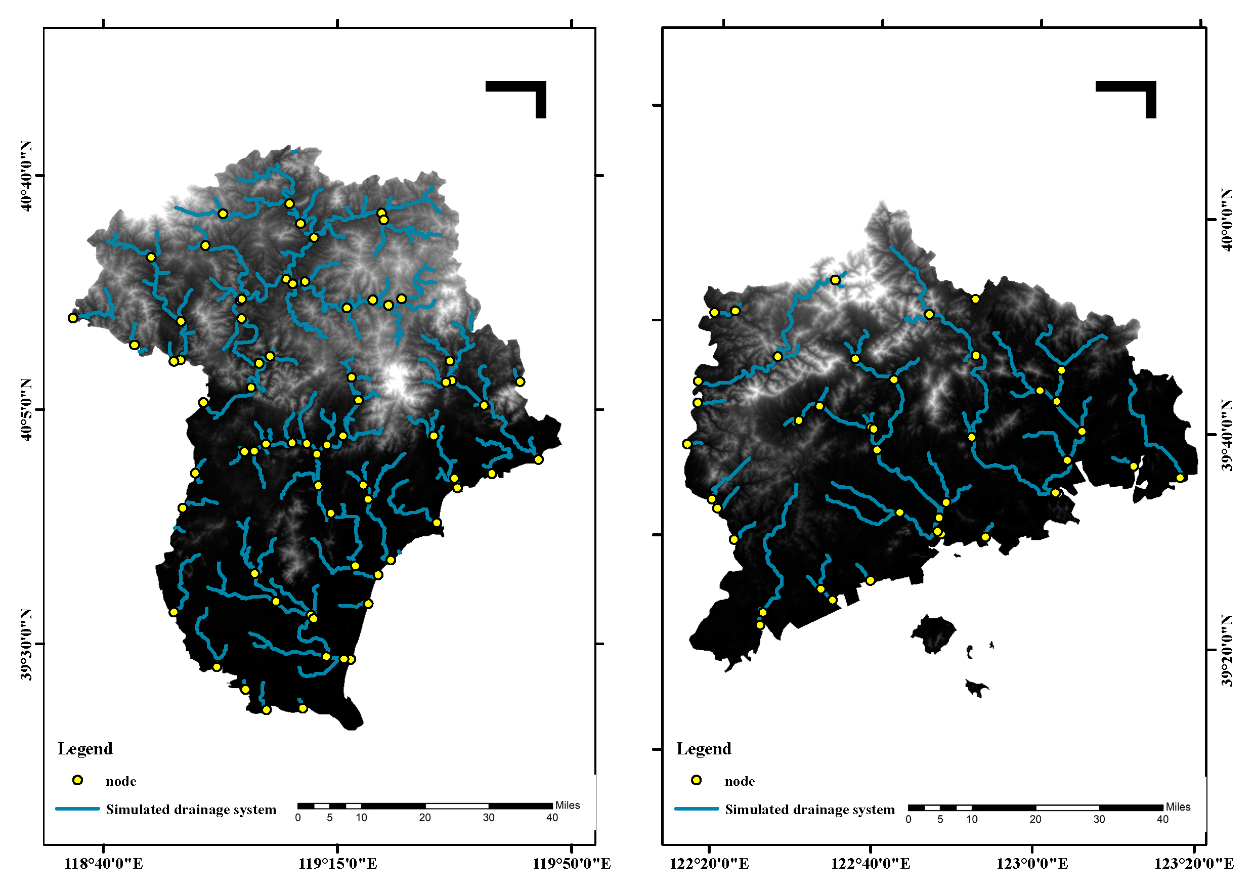
- Node generation: a node is a point where water flows out of an area. This point is usually the lowest point along the boundary of the basin, that is, the point where the accumulated maximum of the internal flow in the catchment area. The river nodes simulated in the model not only reflects the consistency of geographical data, but also provides a guarantee for the subsequent hydrological and geomorphic simulation process analysis. In this paper, the optimal node was selected by combining the distribution of nodes under different thresholds, and eliminating the useless node information, and then the reservoir point information was inputted into the river network node.
2.3.2. Model Calibration and Verification
3. Results and Discussion
3.1. Threshold Determination
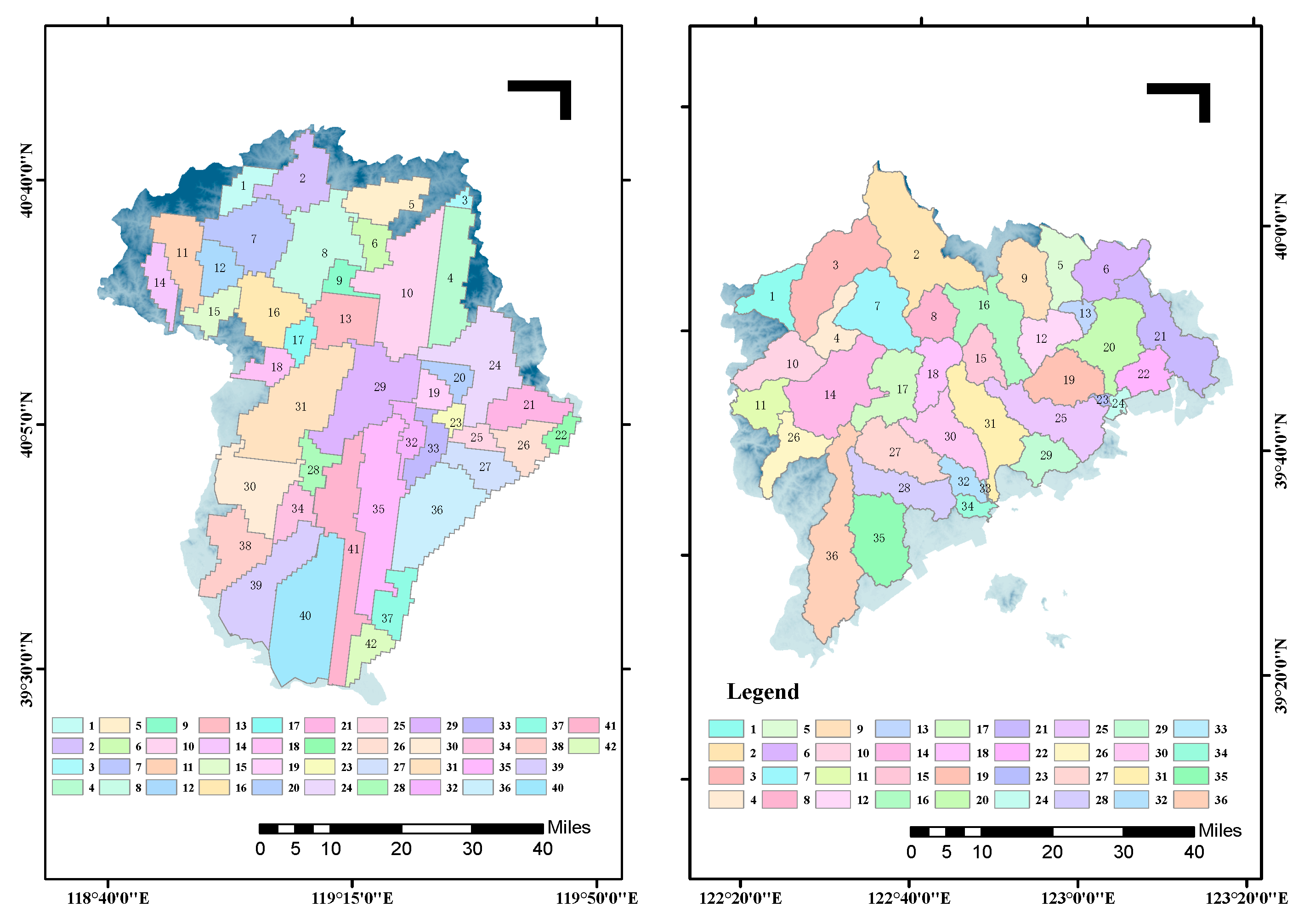
3.2. Sub-Basin Division
3.3. Simulation Calculus
3.3.1. Parameter Sensitivity Analysis and Model Calibration
3.3.2. Analysis and Evaluation of Simulation Results
4. Conclusions
Supplementary Materials
Author Contributions
Funding
Acknowledgments
Conflicts of Interest
References
- Abbott, M.B.; Refsgaard, J.C. Distributed Hydrological Modelling; Kluwer Academic Publishers: Dordrecht, The Netherlands, 1996; pp. 17–39. [Google Scholar]
- Liu, K.; Song, C.; Ke, L.; Jiang, L.; Pan, Y.; Ma, R. Global open-access DEM performances in Earth’s most rugged region High Mountain Asia: A multi-level assessment. Geomorphology 2019, 338, 16–26. [Google Scholar] [CrossRef]
- Zurqani, H.A.; Post, C.J.; Mikhailova, E.A.; Cope, M.P.; Allen, J.S.; Lytle, B.A. Evaluating the integrity of forested riparian buffers over a large area using LiDAR data and Google Earth Engine. Sci. Rep. 2020, 10, 14096. [Google Scholar] [CrossRef] [PubMed]
- Sanzana, P.; Gironas, J.; Braud, I.; Branger, F.; Rodriguez, F.; Vargas, X.; Hitschfeld, N.; Munoz, J.F.; Vicuna, S.; Mejia, A.; et al. A GIS-based Urban and Peri-urban Landscape Representation Toolbox for Hydrological Distributed Modeling. Environ. Model. Softw. 2017, 91, 168–185. [Google Scholar] [CrossRef] [Green Version]
- Freeze, R.A.; Harlan, R.L. Blueprint for a physically–based, digitally–simulated hydrologic response model. J. Hydrol. 1969, 9, 237–258. [Google Scholar] [CrossRef]
- Taye, M.T.; Ntegeka, V.; Ogiramoi, N.P.; Willems, P. Assessment of climate change impact on hydrological extremes in two source regions of the Nile River Basin. Hydrol. Earth Syst. Sci. 2011, 15, 209–222. [Google Scholar] [CrossRef] [Green Version]
- Tian, Y.; Xu, Y.P.; Zhang, X.J. Assessment of Climate Change Impacts on River High Flows through Comparative Use of GR4J, HBV and Xinanjiang Models. Water Resour. Manag. 2013, 27, 367–384. [Google Scholar] [CrossRef]
- Abbott, M.B.; Bathurst, J.C.; Cunge, J.A. An introduction to the System Hydrological European, “SHE”, 1. History and philosophy of a physically–based, distributed modelling system. J. Hydrol. 1986, 87, 45–59. [Google Scholar] [CrossRef]
- Gassman, P.W.; Reyes, M.R.; Green, C.H.; Arnold, J.G. The soil and water assessment tool: Historical development, applications, and future research directions. Trans. Asabe 2007, 50, 1211–1250. [Google Scholar] [CrossRef] [Green Version]
- Xu, L.; Wood, E.F.; Lettenmaier, D.P. Surface soil moisture parameterization of the VIC–2L model: Evaluation and modification. Glob. Planet. Chang. 1996, 13, 195–206. [Google Scholar]
- Wigmosta, M.S.; Vail, L.W.; Lettenmaier, D.P. A distributed hydrology–vegetation model for complex terrain. Water Resour. Res. 1994, 30, 1665–1679. [Google Scholar] [CrossRef]
- Gupta, V.K.; Waymire, E. Multiscaling properties of spatial rainfall and river flow distributions. J. Geophys. Res. Atmos. 1990, 95, 1999–2009. [Google Scholar] [CrossRef]
- Jain, M.K.; Kothyari, U.C.; Raju, K. A GIS based distributed rainfall–runoff model. J. Hydrol. 2004, 299, 107–135. [Google Scholar] [CrossRef]
- Bao, H.; Wang, L.; Li, Z.; Yao, C. A distributed hydrological model based on Holtan runoff generation theory. J. Hohai Univ. Nat. Sci. 2016, 44, 340–346. [Google Scholar]
- Shu, D.; Cheng, G.; Lin, S. Spatial discretization of digital watershed based on DEM for the upper reach of Minjiang River. J. Sichuan Univ. Eng. Sci. Ed. 2004, 36, 6–11. [Google Scholar]
- Fontaine, T.A.; Cruickshank, T.S.; Arnold, J.G.; Hotchkiss, R.H. Development of a snowfall–snowmelt routine for mountainous terrain for the soil water assessment tool (SWAT). J. Hydrol. 2002, 262, 209–223. [Google Scholar] [CrossRef]
- Cambien, N.; Gobeyn, S.; Nolivos, I.; Forio, M.A.E.; Arias–Hidalgo, M.; Dominguez–Granda, L.; Witing, F.; Volk, M.; Goethals, P.L. Using the Soil and Water Assessment Tool to Simulate the Pesticide Dynamics in the Data Scarce Guayas River Basin, Ecuador. Water 2020, 12, 696. [Google Scholar] [CrossRef] [Green Version]
- Senent–Aparicio, J.; Alcalá, F.J.; Liu, S.; Jimeno–Sáez, P. Coupling SWAT Model and CMB Method for Modeling of High–Permeability Bedrock Basins Receiving Interbasin Groundwater Flow. Water 2020, 12, 657. [Google Scholar] [CrossRef] [Green Version]
- Liu, Y.; Cui, G.; Li, H. Optimization and Application of Snow Melting Modules in SWAT Model for the Alpine Regions of Northern China. Water 2020, 12, 636. [Google Scholar] [CrossRef] [Green Version]
- Stone, M.C.; Hotchkiss, R.; Mearns, L.O. Water Yield Responses to High and Low Spatial Resolution Climate Change Scenarios in the Missouri River Basin. Geophys. Res. Lett. 2003, 30, 31–35. [Google Scholar] [CrossRef] [Green Version]
- Wang, Y.; Shao, J.; Su, C.; Cui, Y.; Zhang, Q. The Application of Improved SWAT Model to Hydrological Cycle Study in Karst Area of South China. Sustainability 2019, 11, 5024. [Google Scholar] [CrossRef] [Green Version]
- Li, T.; Guo, S.; An, D.; Nametso, M. Study on water and salt balance of plateau salt marsh wetland based on time–space watershed analysis. Ecol. Eng. 2019, 138, 160–170. [Google Scholar] [CrossRef]
- Huang, J.; Wen, J.; Wang, B.; Hinokidaniet, O. Structural Universality of the Distributed Hydrological Model for Small–and Medium–Scale Basins with Different Topographies. J. Hydrol. Eng. 2018, 23, 04017054. [Google Scholar] [CrossRef]
- Turcotte, R.; Fortin, J.P.; Rousseau, A.N.; Massicotte, S.; Villeneuve, J.P. Determination of the drainage structure of a watershed using a digital elevation model and a digital river and lake network. J. Hydrol. 2001, 240, 225–242. [Google Scholar] [CrossRef]
- Liu, H.; Du, J.; Jia, Y.; Liu, J.; Niu, C.; Gan, Y. Improvement of watershed subdivision method for large scale regional distributed hydrology model. Adv. Eng. Sci. 2019, 51, 36–44. [Google Scholar]
- Li, Y.; Yang, X.; Long, W. Topographic Dependence of Cropland Transformation in China during the First Decade of the 21st Century. Sci. World J. 2013, 2013, 303685. [Google Scholar] [CrossRef]
- Saxton, K.; Willey, P. Watershed Models; CRC Press: Boca Raton, FL, USA, 2006; pp. 400–435. [Google Scholar]
- Meng, X.; Wang, H.; Shi, C.; Wu, Y.; Ji, X. Establishment and Evaluation of the China Meteorological Assimilation Driving Datasets for the SWAT Model (CMADS). Water 2018, 10, 1555. [Google Scholar] [CrossRef] [Green Version]
- Meng, X.Y.; Yu, D.L.; Liu, Z.H. Energy balance–based SWAT model to simulate the mountain snowmelt and runoff–taking the application in Juntanghu watershed (China) as an example. J. Mt. Sci. 2015, 12, 368–381. [Google Scholar] [CrossRef]
- Arabi, M.; Govindaraju, R.S.; Hantush, M.M. A probabilistic approach for analysis of uncertainty in the evaluation of watershed management practices. J. Hydrol. 2007, 333, 459–471. [Google Scholar] [CrossRef]
- Martz, L.W.; Garbrecht, J. An outlet breaching algorithm for the treatment of closed depressions in a raster DEM. Comput. Geosci. 1999, 25, 835–844. [Google Scholar] [CrossRef]
- O’Callaghan, J.F.; Mark, D.M. The extraction of drainage networks from digital elevation data. Comput. Vis. Graph. Image Process. 1984, 27, 323–344. [Google Scholar] [CrossRef]
- Qiu, J.; Shen, Z.; Huang, M.; Zhang, X. Exploring effective best management practices in the Miyun reservoir watershed, China. Ecol. Eng. 2018, 123, 30–42. [Google Scholar] [CrossRef]
- Nash, J.E.; Sutcliffe, J.V. River flow forecasting through conceptual models part I–A discussion of principles. J. Hydrol. 1970, 10, 282–290. [Google Scholar] [CrossRef]
- Giannoni, F.; Roth, G.; Rudari, R. A procedure for drainage network identification from geomorphology and its application to the hydrologic response. Adv. Water Resour. 2005, 28, 567–581. [Google Scholar] [CrossRef]
- Zhang, J.; Tang, L.; Xie, T.; Peng, Q. Determination of catchment area threshold for extraction of digital river–network. Water Resour. Hydropower Eng. 2016, 47, 1–4. [Google Scholar]
- Lin, W.T.; Chou, W.C.; Lin, C.Y.; Huang, P.H.; Tsai, J.S. Automated suitable drainage network extraction from digital elevation models in Taiwan’s upstream watersheds. Hydrol. Process. 2006, 20, 289–306. [Google Scholar] [CrossRef]
- Oudin, L.; Andréassian, V.; Mathevet, T.; Perrin, C.; Michel, C. Dynamic averaging of rainfall–runoff model simulations from complementary model parameterizations. Water Resour. Res. 2006, 42, 887–896. [Google Scholar] [CrossRef]
- Meng, F.; Sa, C.; Liu, T.; Luo, M.; Liu, J.; Tian, L. Improved Model Parameter Transferability Method for Hydrological Simulation with SWAT in Ungauged Mountainous Catchments. Sustainability 2020, 12, 3551. [Google Scholar] [CrossRef]


| Study Area | Precision | Latitude | Climate |
|---|---|---|---|
| Qinhuangdao | 118°33′ E–119°51′ E | 39°24′ N–40°37′ N | Temperate continental monsoon climate |
| Zhuanghe | 122°29′ E–123°31′ E | 39°25′ N–40°12′ N | Temperate monsoon climate |
| Study Area | Grade Classification (Unit/Degree) | Maximum Slope | Standard Deviation of Slope | Average Slope | Maximum Elevation | Average Elevation | |||||
|---|---|---|---|---|---|---|---|---|---|---|---|
| ≤5 | 5–10 | 10–15 | 15–30 | 30–50 | 50–70 | ||||||
| Qinhuangdao | 30.63% | 12.94% | 14.57% | 39.45% | 2.40% | 0.02% | 68.14 | 8.50 | 12.01 | 1823.00 | 228.49 |
| Zhuanghe | 55.55% | 19.80% | 11.15% | 12.62% | 0.88% | 0.00% | 54.43 | 6.96 | 6.55 | 1090.00 | 101.83 |
| Study Area | Cultivated Land | Forest | Water | Urban | Pasture | Other Land |
|---|---|---|---|---|---|---|
| Qinhuangdao | 40.92% | 38.90% | 6.30% | 10.23% | 2.32% | 1.33% |
| Zhuanghe | 49.47% | 30.55% | 7.18% | 9.39% | 1.45% | 1.96% |
| Soil Grouping | Soil and Water Assessment Tool (SWAT) Code | Harmonized World Soil Database (HWSD) Name | Qinhuangdao | Zhuanghe | ||
|---|---|---|---|---|---|---|
| Percentage | Hydrological Group (HYDGRP) | Percentage | HYDGRP | |||
| ARENOSOLS | ARh | Haplic Arenosols | 0.59% | A | – | – |
| ANTHROSOLS | ATc | Cumulic Anthrosols | 0.35% | C | 8.56% | C |
| CAMBISOLS | CMc | Calcaric Cambisols | 13.63% | B | – | – |
| CMe | Eutric Cambisols | 18.98% | B | 4.70% | B | |
| FLUVISOLS | FLc | Calcaric Fluvisols | 16.25% | A | – | – |
| FLs | Salic Fluviosls | 0.31% | B | – | – | |
| LEPTOSOLS | LPe | Eutric Leptosols | 0.89% | B | – | – |
| GLEYSOLS | GLe | Eutric Gleysols | – | – | 3.40% | B |
| LUVISOLS | LVa | Albic Luvsiols | – | – | 0.21% | B |
| LVg | Gleyic Luvisols | 14.60% | B | 9.44% | B | |
| LVh | Haplic Luvisols | 13.90% | B | 50.01% | B | |
| LVk | Calcic Luvisols | 4.65% | A | – | – | |
| REGOSOLS | RGc | Calcaric Regosols | 3.43% | B | – | – |
| RGe | Eutric Regosols | 11.49% | B | – | – | |
| SOLONCHAKS | SCh | Haplic Solonchaks | 0.94% | A | 2.39% | C |
| PHAEOZEMS | PHg | Gleyic Phaeozems | – | – | 0.09% | D |
| PHh | Haplic Phaeozems | – | – | 21.22% | B | |
| Threshold (ha) | River Length (km) | Basin Area (km2) | Drainage Density (km–1) | |||
|---|---|---|---|---|---|---|
| Qinhuangdao | Zhuanghe | Qinhuangdao | Zhuanghe | Qinhuangdao | Zhuanghe | |
| 1000 | 4870.120 | 2822.881 | 6602.230 | 3400.167 | 0.738 | 0.830 |
| 2000 | 3019.130 | 1961.631 | 6501.520 | 3340.123 | 0.464 | 0.587 |
| 3000 | 2214.230 | 1581.13 | 6450.430 | 3300.224 | 0.343 | 0.479 |
| 4000 | 1742.280 | 1352.879 | 6400.770 | 3240.332 | 0.272 | 0.418 |
| 5000 | 1485.767 | 1204.609 | 6301.510 | 3200.123 | 0.236 | 0.376 |
| 6000 | 1255.360 | 1117.759 | 6254.630 | 3157.800 | 0.201 | 0.354 |
| 7000 | 1098.979 | 1001.717 | 6200.450 | 3075.760 | 0.177 | 0.326 |
| 8000 | 1018.597 | 939.218 | 6214.550 | 3065.770 | 0.164 | 0.306 |
| 9000 | 947.251 | 890.957 | 6200.340 | 3055.130 | 0.153 | 0.292 |
| 10,000 | 876.235 | 837.242 | 6189.320 | 3045.440 | 0.142 | 0.275 |
| Parameters | Physical Meaning of Parameters [39] | t–Stat | p–Value | Sensitivity Priority | Revised Scheme | Range | Optimum Value | |||||
|---|---|---|---|---|---|---|---|---|---|---|---|---|
| Q | Z | Q | Z | Q | Z | Q | Z | – | Q | Z | ||
| CN2 | Initial SCS runoff curve number for moisture condition II | 12.58 | 14.72 | 0 | 0 | 1 | 1 | R | R | −0.2–0.2 | 0.35 | 0.35 |
| GW_REVAP | Groundwater “revap” coefficient | −1.76 | 1.79 | 0.08 | 0.08 | 5 | 4 | V | R | 0.02–0.2 | 0.16 | 0.09 |
| GW_DELAY | Groundwater delay time (days) | −2.38 | −2.05 | 0.03 | 0.04 | 3 | 3 | V | V | 30.0–450.0 | 243 | 75.1 |
| GWQMN | Threshold depth of water in the shallow aquifer required for return flow to occur (mm H2O) | 2.04 | −1.83 | 0.07 | 0.1 | 4 | 5 | V | V | 0.0–5000.0 | 2671 | 696.24 |
| ALPHA_BF | Baseflow alpha factor (1/days) | −3.53 | 0.028 | 0.01 | 0.97 | 2 | 14 | V | V | 0.0–1.0 | 0.56 | 0.58 |
| ESCO | Soil evaporation compensation factor | −1.33 | −0.72 | 0.22 | 0.46 | 6 | 10 | V | V | 0.01–1.0 | 0.51 | 0.64 |
| EPCO | Plant uptake compensation factor | −0.87 | 0.78 | 0.37 | 0.5 | 7 | 9 | V | R | 0.01–1.0 | 0.53 | 0.97 |
| CH_N2 | Manning’s “n” value for the main channel | −0.85 | −0.91 | 0.39 | 0.42 | 8 | 8 | V | R | 0.0–0.3 | 0.18 | 0.18 |
| CH_K2 | Effective hydraulic conductivity in main channel alluvium (mm/h) | 0.84 | −1.30 | 0.4 | 0.23 | 9 | 6 | V | R | 5.0–130.0 | 124 | 77.19 |
| SOL_AWC | Available water capacity of the soil layer (mm H2O/mm soil) | −0.7 | −2.79 | 0.49 | 0.02 | 10 | 2 | R | R | −0.5–0.5 | 0.2 | −0.16 |
| SOL_K | Saturated hydraulic conductivity (mm/hr) | −0.52 | −0.47 | 0.64 | 0.65 | 11 | 11 | R | R | −0.8–0.8 | 0.28 | −0.38 |
| REVAPMN | Threshold depth of water in the shallow aquifer for “revap” or percolation to the deep aquifer to occur (mm H2O) | 0.31 | −0.85 | 0.55 | 0.43 | 12 | 7 | V | R | 0.0–500.0 | 258 | 22.08 |
| Study Area | Rate Regular | Validation Period | ||||
|---|---|---|---|---|---|---|
| NSE | R2 | Re | NSE | R2 | Re | |
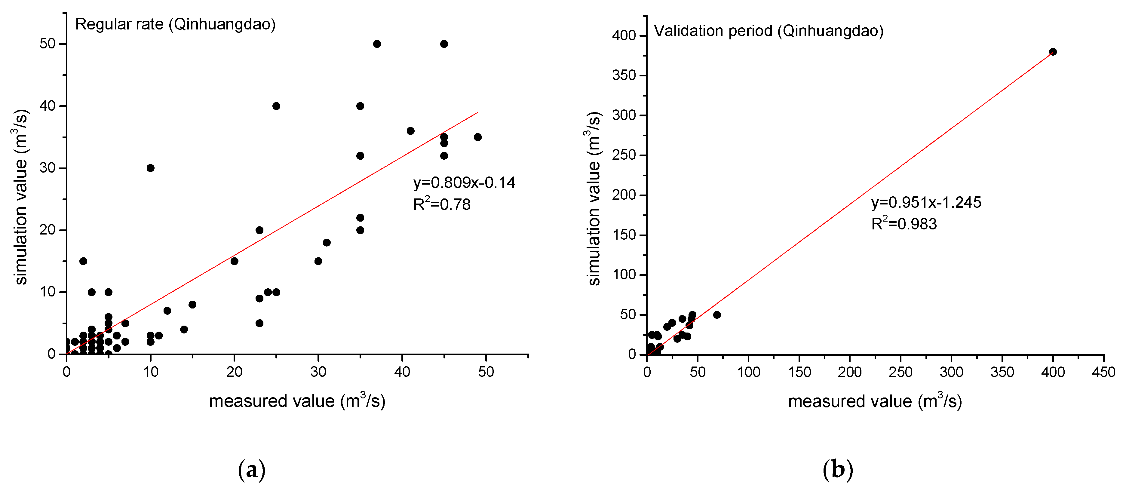
| Qinhuangdao | 0.78 | 0.78 | 4.89% | 0.90 | 0.980 | 3.99% |
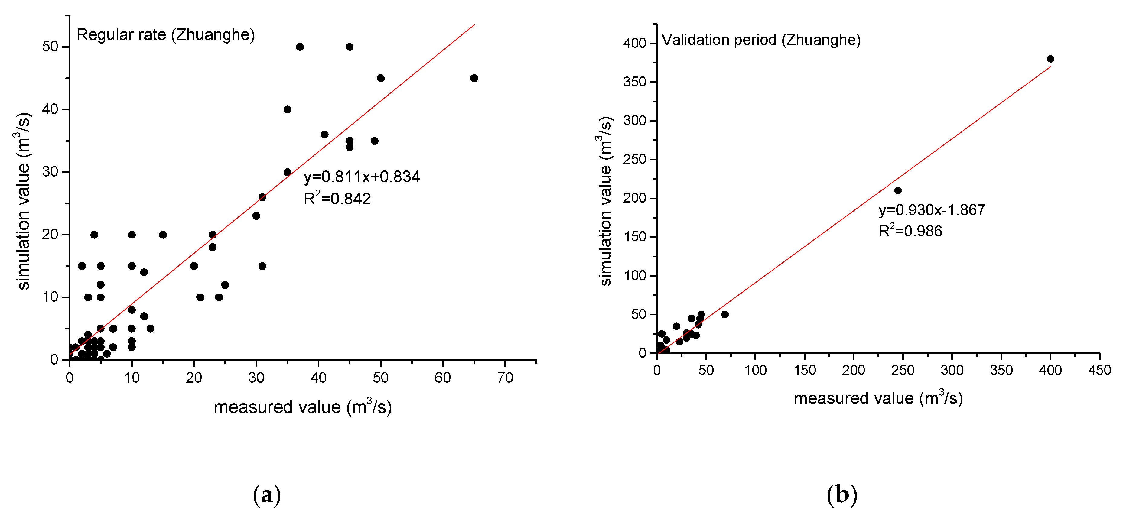
| Zhuanghe | 0.88 | 0.84 | 3.80% | 0.91 | 0.984 | 1.30% |
Publisher’s Note: MDPI stays neutral with regard to jurisdictional claims in published maps and institutional affiliations. |
© 2020 by the authors. Licensee MDPI, Basel, Switzerland. This article is an open access article distributed under the terms and conditions of the Creative Commons Attribution (CC BY) license (http://creativecommons.org/licenses/by/4.0/).
Share and Cite
Li, T.; Duan, Y.; Guo, S.; Meng, L.; Nametso, M. Study on Applicability of Distributed Hydrological Model under Different Terrain Conditions. Sustainability 2020, 12, 9684. https://doi.org/10.3390/su12229684
Li T, Duan Y, Guo S, Meng L, Nametso M. Study on Applicability of Distributed Hydrological Model under Different Terrain Conditions. Sustainability. 2020; 12(22):9684. https://doi.org/10.3390/su12229684
Chicago/Turabian StyleLi, Tianxin, Yuxin Duan, Shanbo Guo, Linglong Meng, and Matomela Nametso. 2020. "Study on Applicability of Distributed Hydrological Model under Different Terrain Conditions" Sustainability 12, no. 22: 9684. https://doi.org/10.3390/su12229684