An Assessment of Environmental Impacts on the Ecosystem Services: Study on the Bagmati Basin of Nepal

1
Department of Advanced Science and Technology Convergence, Kyungpook National University, 2559, Gyeongsangdaero, Sangju 37224, Korea
2
School of Agricultural Civil & Bio-Industrial Engineering, Kyungpook National University, 80 Daehak-ro, Buk-gu, Daegu 41566, Korea
*
Author to whom correspondence should be addressed.
Sustainability 2020, 12(19), 8186; https://doi.org/10.3390/su12198186
Submission received: 10 August 2020
/
Revised: 27 September 2020
/
Accepted: 28 September 2020
/
Published: 4 October 2020
(This article belongs to the Special Issue Hydrological Responses by Climate Change and Human Activities)
Abstract
:The upsurges in population, internal migration, and various development works have caused significant land use and land cover (LULC) changes in the Bagmati Basin of Nepal. The effects of climate change such as increased precipitation and temperature are affecting the provision of ecosystem services (ES). In this regard, this study particularly treated water yield (WY), soil loss, nitrogen export, and carbon fluctuation in the basin. Integrated Valuation of Ecosystem Services and Tradeoffs (InVEST) tools were used to carry out a comparative analysis of ES based on LULC data for 2000 and 2010 and corresponding climate data. To analyze the future period (2010–2099), we have used climate data from the multi-model ensemble (MME) of statistically downscaled and bias-corrected 12 best global climate models (GCMs). A raw GCM analysis (based on historical observational data) from 29 GCMs was done first. The results shows with a subsequent degradation of ES providers like forests and an increment in agricultural and urban areas, ES are on a verge of degradation. Furthermore, a projection of future climate patterns depicts increased precipitation and temperature. Thus, urgent measures are required for the sustainable provision of ES. Outcomes of the study are expected to help in the incorporation of ES in development policies promoting low-impact development along with maintaining ecological and economic goals. The study closes by presenting a recommendation for model application and future study needs.
1. Introduction
Ecosystem services (ES) are defined as services provided by nature that directly and indirectly benefit the well-being of humans. The concept of ES has been developed in the scientific literature since the end of the 1970s [1], and the Millennium Ecosystem Assessment (MEA) report 2005 [2] is considered the milestone in the field of mapping ES. The MEA report evaluated the impacts on human beings as the consequences of changes in the ecosystem. The core finding of the MEA report is that human activities are depleting the Earth’s natural resources, which is inducing stress on the self-sustaining capability of the natural environment. This phenomenon urges immediate measures for checking and prevention in order to enhance the sustainability of ecosystems for future generations.
To meet the requirements of a globally increasing population for food, shelter, timber, etc., land use changes are occurring but at the expense of a degraded environment and ecosystems. Land use and land cover (LULC) change is considered the major factor for the degradation of ES and loss in biodiversity [3,4]. Climate change is another factor impacting natural systems, and ultimately affects the flow of ES [5]. With the increasingly evident effects of climate change, which is especially impacting developing countries [6,7,8], the challenge to attain sustainable economic development goals while preserving the natural resources and ES is getting more difficult [9]. ES have significance in both developed and developing nations. However, as the livelihood of people in developing nations is highly dependent on them, the risk of ES losses is high in developing nations. In addition, developing nations are more prone to the impacts of climate change. In this scenario, identifying where ES originate and to whom the benefits flow under current and future climate conditions is critical information [9].
Land cover refers to the biophysical attributes of Earth’s surface such as water, soil, vegetation, etc. It refers to human purposes or intents applied to these attributes such as building construction, forestry, etc. [10]. Changes in LULC is a substantial phenomenon and is occurring globally since time immemorial [11]. Urbanization is necessary for regional economic growth [12] and is one of the most important drivers of change worldwide [13]. The recent decade has seen a major increase in the rate of worldwide urbanization. As per the 2011 census of the Central Bureau of Statistics of Nepal, the urban population has increased to 17% in 2011 from 2.9% in 1952/1954 [14]. Recorded among the fastest urbanizing countries of the world [15], Nepal has faced notable LULC changes especially in urban and semi-urban areas. The Bagmati Basin, incorporating the capital city Kathmandu, has significant socio-economic importance because of centralized job opportunities, education, health facilities, etc. Issues such as decreased availability of freshwater resources, urban floods, degraded water quality, solid waste management, etc. are major problems in the basin especially in urban and semi-urban areas in the upper part of the basin [16]. The basin has been facing many flood events in its lower belt [16] and urban floods have become a re-occurring phenomenon every monsoon season in major city cores like in Kathmandu and Bhaktapur. Water availability and accessibility are also issues and due to the lack of effective plans for waste management by households, industries, and agricultural areas, water quality is on the constant verge of degradation [17]. Likewise, unchecked LULC changes for activities such as agriculture and road expansion are increasing soil loss rates. Industrialization and urbanization mainly in the upper part of the basin are impacting the overall ES of the basin. The optimum provision of ES under changing LULC and climatic conditions would be questionable if proper mitigation and preservation plans are not formulated in time.
Several studies on ES have been carried out in Nepal to inform biodiversity conservation and to promote local and national decision making [18,19]. Some examples are LULC dynamics and ES valuation in the Gandaki Basin of Nepal [20] and effects of LULC change on ES in the Koshi Basin, which focused on food production, carbon storage, habitat quality, etc. [21]. Several international organizations such as the International Union for Conservation of Nature (IUCN), the International Centre for Integrated Mountain Development (ICIMOD), the World Bank, and the Asian Development Bank are currently working toward the assessment of ES and the implementation of Payments for Ecosystem Services (PES) in Nepal [19,22]. The implementation of PES schemes in sectors such as drinking water, irrigation, and tourism already exists in Nepal, but these payments are being made only for mandatory requirements, not for the sustained supply of services [19]. Many studies have independently assessed freshwater availability [23], water pollution issues [24], and soil loss cases [25] in the Bagmati Basin of Nepal. However, to the extent of our knowledge, a collective effort to access in terms of ES, LULC impacts on them, and projections based on climate data are not yet available. Thus, to overcome this gap, the concept of this study was devised. Climate change and LULC are major drivers of changes in ES and ES are itself interrelated [26]. This study aims to analyze the impacts on ES owing to changes in LULC and to provide an overview of the provision of ES in the context of a changing climate. This study thus treats four regulating ES, namely, water yield (WY) for a freshwater provision and flood control, soil loss indicating soil degradation and impacts on interrelated services, nitrogen export for surface water quality, and carbon storage for climate regulation. Integrated Valuation of Ecosystem Services and Tradeoffs (InVEST) [27] ES tools and the Revised Universal Soil Loss Equation (RUSLE) [28] method along with ArcGIS were used to map ES of the basin, and APCC Integrated Modelling Solution (AIMS) software developed by the Asia Pacific Economic Cooperation Climate Centre (APCC) was used for statistical downscaling of bias-corrected global climate model (GCM) data.
2. Materials and Methods
2.1. Study Area
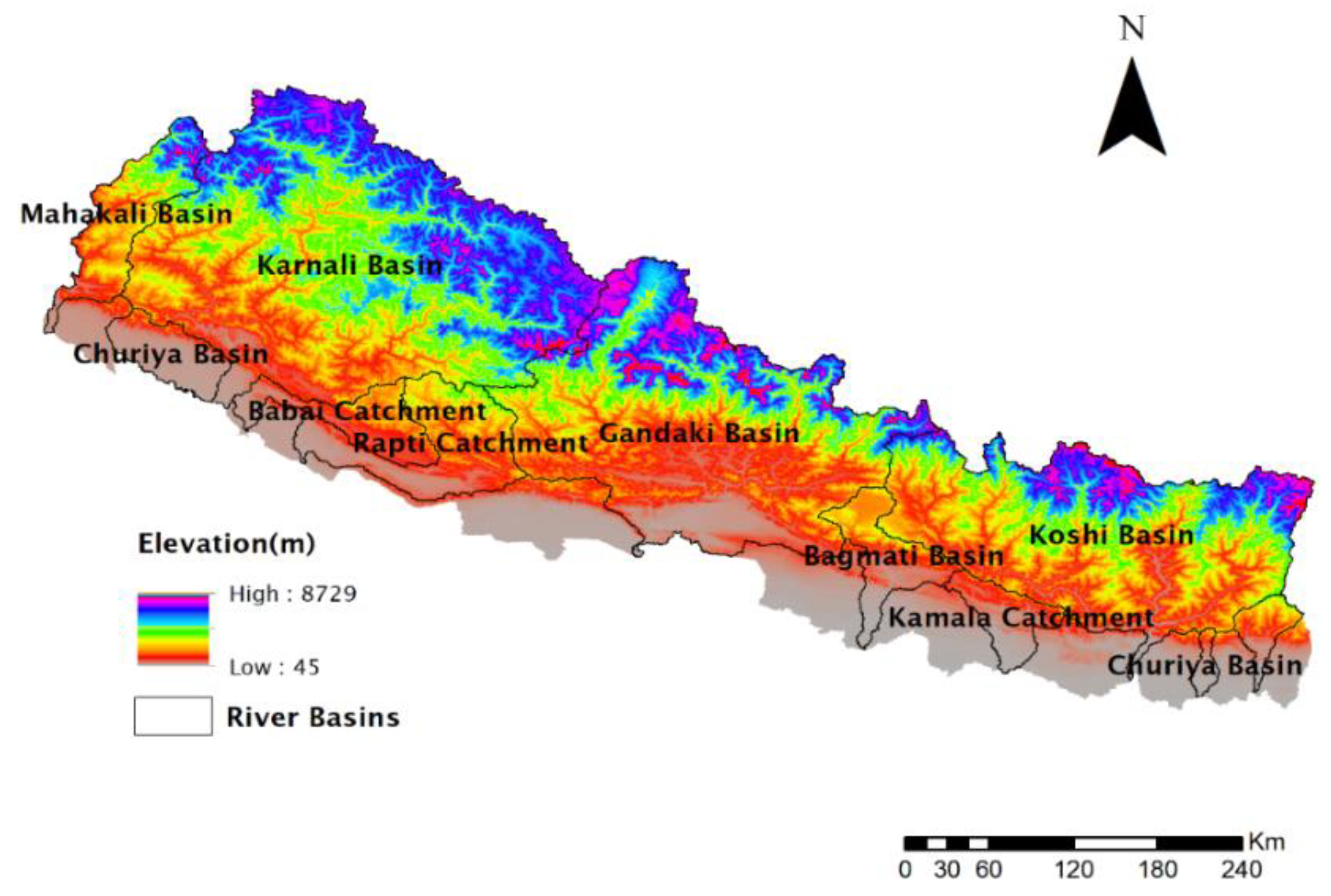
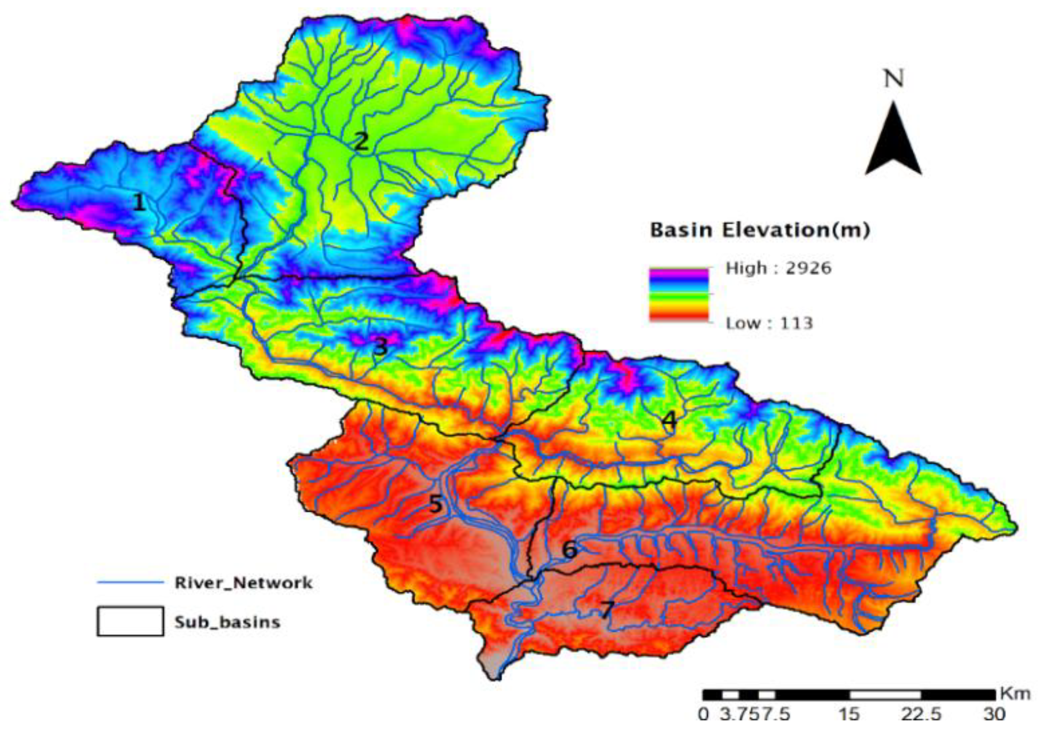
The Bagmati Basin lies in the middle mountain region of Nepal (Figure 1) at latitude 26°42′ to 27°50′ N and longitude 85°2′ to 85°58′ E. The Bagmati River is the principal river of the basin and it originates from the north of the capital city, Kathmandu, at Shivpuri (Bagdwar) at an altitude of 2690 m. The river flows through Kathmandu and provides most of the city’s drinking water in the upper part of the basin, supports hydropower generation in the middle basin and in the lower part of the basin, and supports large-scale irrigation for agriculture [29]. The climate of the basin varies with elevation; higher mountains have a cold temperate climate, mid-elevation levels have a warm temperate climate, and the southern lowlands have a subtropical climate [30]. The basin has a mean annual temperature of 20–30 °C and the mean annual precipitation is about 1800 mm [30]. The Bagmati River is a spring and monsoon rain-fed river and consists of many tributaries such as the Hanumante, Manohara, Dhobi Khola, etc. The total area of the basin is 375,000 ha and, owing to the good data availability for this study, a 276,897 ha area was selected. This represents the area above the Pandredhovan gauge station (Figure 2). We chose the Bagmati Basin as our study area as it is facing huge anthropogenic pressures associated mostly with centralized facilities, urban expansion, and increased agricultural activity.
2.2. Model Description and Data
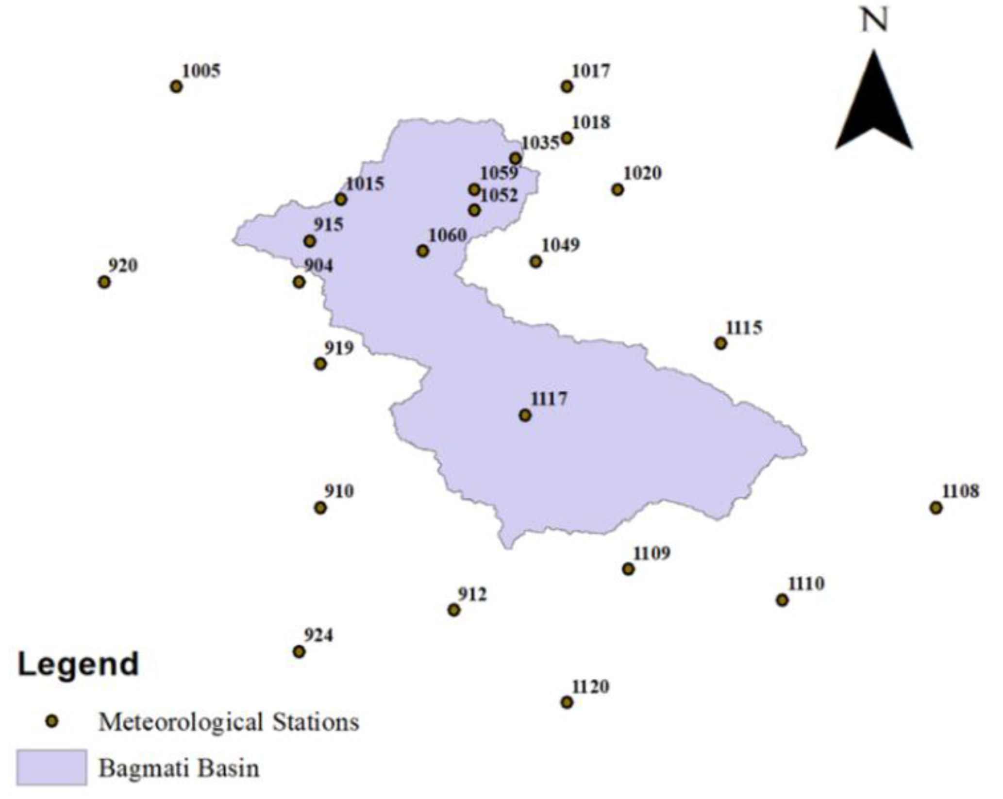
For the assessment of ES provision in the basin, four ES, namely, WY, soil loss, nitrogen export, and carbon storage, were evaluated on the sub-basin scale in the Bagmati Basin of Nepal. We have done a comparative study of ES for the years 2000 and 2010 based on the LULCs of 2000 and 2010 and corresponding climate data and for a future period, ES were mapped based on the LULC map of 2010 and projected climate data. The LULC map was obtained from the ICIMOD Nepal Geospatial Portal (http://rds.icimod.org/) which is prepared using public domain Landsat Thematic mapper(TM) data. Uddin et al. [31] have discussed the detailed description of the data including LULC classification, accuracy assessment, and limitations, hence we have used the LULC data from the ICIMOD portal referring to the findings from Uddin et al. [31]. Likewise, the rainfall and temperature data for the period of 1987–2016 from 25 stations from all over Nepal (Table S1, Supplementary Materials) have been used to downscale GCM data for Nepal. The missing data were extracted from MERRA2 grid data [32] after doing quality control (checking daily correlation coefficient) using R package. GCM data from 10 stations (stations in bold in Table S1, Supplementary Materials) have been used for a future period (2010–2099) ES evaluation of the Bagmati Basin. As well, for the analysis of the Bagmati Basin for the period 2000 and 2010, a precipitation raster is prepared using data from 23 rain stations (Figure 3) and, for preparation of an evapotranspiration raster, precipitation and temperature data from 9 stations (stations in bold in Table S1, Supplementary Materials) have been used. The data period for the comparative study of 2000 and 2010 is 1996–2015 which is divided into two time periods of 1996–2005 and 2006–2015 to coincide with available LULC data of 2000 and 2010 periods, respectively. All the rainfall and temperature data were acquired from the Department of Hydrology and Meteorology (DHM) Nepal.
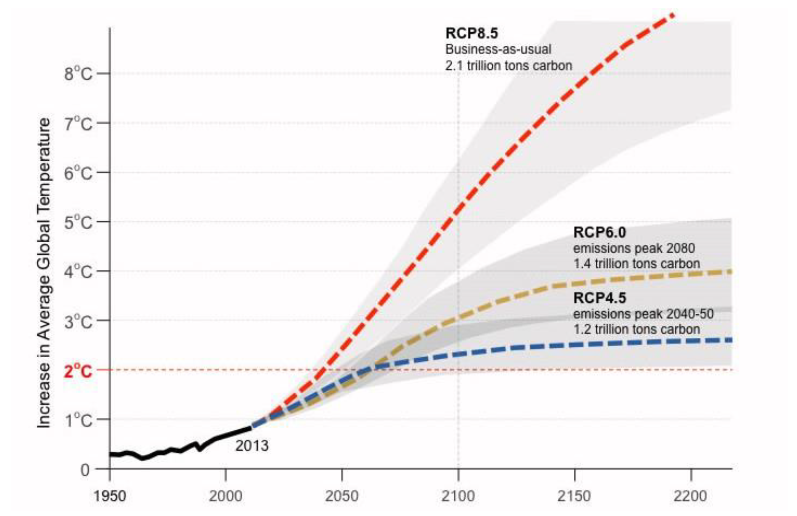
For the downscaling of GCMs for future climate data, we have used APCC’s AIMS software. We have used the multi-model ensemble (MME) of 12 best GCMs of Coupled Model Intercomparison Project 5 (CMIP5) under two Representative Concentration Pathways (RCP) scenarios namely RCP 4.5 and RCP 8.5 to study the projection of ES in the future. The descriptions of RCP 4.5 and RCP 8.5 are given in Figure 4. InVEST tools were used to map WY, nitrogen export, and carbon storage, and a RUSLE method was used to map soil loss. As carbon storage computation by the InVEST carbon model is independent of the climate data, carbon storage was evaluated with only LULC change and the corresponding climate scenario whereas WY, soil loss, and nitrogen export were evaluated for both scenarios of LULC change and future climate change scenarios. We choose the InVEST model in our study due to its capability to give a quick overview of ES, especially in regions with low data availability [33] in developing nations like Nepal. InVEST is a suite of a free and open source software models. Its modular design provides an effective tool for evaluating the possible outcomes of alternative management and climate scenarios and it helps in the selection of the best decision scenarios [27].
2.2.1. Water Yield Estimation
The InVEST water yield model was used for the WY estimation and this model is based on the water balance principle and Budyko curve. It determines the amount of water running off each pixel as the precipitation minus the fraction of the water that undergoes evapotranspiration. The input data included precipitation, evapotranspiration, LULC, soil properties, basin boundary, and biophysical attributes (Table 1). The spatial resolution of LULC, soil depth, and plant-available water content used in the study was 30 m.
The annual WY Y(x) on each pixel of the landscape (x) is determined as follows:
- AET(x) = Annual actual evapotranspiration for pixel x
- P(x) = Annual precipitation on pixel x.
is the evapotranspiration portion of the water balance for vegetated LULC types. This is computed based on an expression of the Budyko curve proposed by Fu [34] and Zhang et al. [35]:
where PET(x) = potential evapotranspiration calculated using Equation (3); ω(x) = non-physical parameter (characterizes the natural climatic-soil properties). Calculation of PET is as follows:
where = reference evapotranspiration from pixel x.
= plant evapotranspiration coefficient, which is associated with the LULC on pixel x.
ω(x) is an empirical parameter. It is determined as the expression given by Donohue et al. [36]:
where ω(x) is based on plant-available water content (PAWC), precipitation, and the Z constant.
The Z constant defines the local precipitation pattern and additional hydrogeological characteristic of the basin [27].
The temperature-based Hargreaves equation was used for the computation of reference evapotranspiration, given that this method generates superior results to the Pennman–Montieth method in the case when long-term data is limited [37]. An average soil depth and PAWC raster map was prepared using the Soil and Terrain (SOTER) database of Nepal and ArcGIS. The biophysical information on the LULC code and its descriptive names, the maximum root depth for vegetated land use classes in mm, and the plant evapotranspiration coefficient for each LULC class was required (Table 2). In this study, the root depth of main vegetation types was obtained following Chen et al. [38] and the evapotranspiration coefficient of each LULC type used on the model was based on Allen et al. [39] and the InVEST user manual [27].
2.2.2. Soil Loss Estimation
The RUSLE model coupled with ArcGIS was used for the computation of soil loss in the basin. Due to data simplicity and the provision of scenario analysis and taking measures against erosion, RUSLE is widely used at large scales for soil loss assessment [40]. It computes soil erosion as the product of six factors representing rainfall erosivity, soil erodibility, slope length, slope steepness, cover and management practices, and supporting conservation practices:
where
- A = average annual soil loss amount in (t/ha/yr)
- R = rainfall–runoff erosivity factor (MJ mm/h/ha/yr)
- K = soil erodibility factor
- L = slope length factor
- S = slope steepness factor
- C = land cover management factor
- P = support practice factor
Among several equations available for the rainfall–runoff erosivity factor (R), we have used the equation by Singh et al. [41] as it is the one recommended for the Himalayan region:
where
- R = rainfall erosivity factor (MJ mm ha−1 h−1 yr−1)
- P = mean annual precipitation (mm).
The K factor is determined as per the Food and Agriculture Organization (FAO) database adapted to Nepal by World Soil Information (ISRIC). The soil unit map was extracted from the SOTER database of Nepal and the K factor was computed based on different published literature on mountainous areas [42,43] and other countries [44]. The K factor of the study area varied from 0.19 to 0.49.
The slope formula based on slope length was used for computation of slope length factor (L) based on references [45,46] which is given as:
where λ indicates a field slope length and 22.13 is the slope length of a unit runoff plot (m).
m = slope length exponent.
The slope steepness factor (S) represents the effect of slope steepness on the intensity of soil erosion. The factor is calculated using Equation (8) as described by Wischmeier and Smith [45]:
where s = slope in percent, which is determined from a digital elevation model (DEM).
Likewise, the cover management factor (C) and the support practice factor (P) were obtained from various published reports [25,47] in a similar area. Separate raster layers for each factor were prepared in GIS and the average annual soil erosion rate was determined by multiplying the respective factors in the ArcGIS environment.
2.2.3. Nitrogen Export Estimation
The nutrient delivery ratio (NDR) model was used to map nitrogen export in the basin. The model uses a simple mass balance approach and describes the movement of nutrient mass through space and aims to quantify nutrient (nitrogen and phosphorous) export. The model maps the flow of nutrients from various sources to the stream network. Sources of nutrients are determined based on a LULC map and associated loading rates. The nutrient loads are divided into sediment-bound and dissolved parts, which will be carried by surface and subsurface flow respectively and stops when they reach a stream. Next, the delivery factors were computed for each pixel, based on the properties of pixels belonging to the same flow path (their slope and retention efficiency of each land use) [27]. All pixel-level contributions were summed at the basin/sub-basin outlet to compute the nutrient export:
where
- = total export amount of nutrients in the basin (kg. yr−1)
- = export amount of nutrients from each grid
- = surface nutrient load (kg. ha−1. yr−1)
- = subsurface nutrient load (kg. ha−1. yr−1)
- = surface nutrient transfer rate.
- = subsurface nutrient transfer rate.
The raster layers required as an input for running the model are raster maps of the DEM, LULC, and precipitation. The model requires the biophysical table having a coefficient for nitrogen loading for each LULC category (Table 2). These values were obtained following Sharp et al. [27] and Line et al. [48].
2.2.4. Carbon Storage Estimation
The InVEST carbon model used in this study maps carbon storage densities to the LULC raster by aggregating the amount of carbon stored on four major carbon pools. The carbon pools considered were aboveground biomass, belowground biomass, soil, and dead organic matter to produce the total amount of carbon storage.
The carbon storage for a given grid cell (i, j) with land use type m can be calculated as:
where A = actual area of each grid cell (ha); Cam,I,j, Cbm,I,j, Csm,I,j, Cdm,I,j are the aboveground, belowground, soil organic, and dead organic matter carbon density in MgC/ha for grid cell (i, j) with land use type m (Table 2). The carbon pool data were obtained from published literature [49,50] and InVEST user guidelines.
2.3. GCM Downscaling and Future Climate Scenarios
For this study, 29 GCMs of CMIP5 were statistically downscaled and bias-corrected using the simple quantile mapping (SQM) [51] method. We adopted RCP 4.5 and RCP 8.5 concentration pathways (Table 3, adapted from reference [52]) for this study. The future projections of daily precipitation and temperature were performed at 25 meteorological stations of Nepal. Statistical downscaling makes it possible to perform a quantitative comparison with observational data through bias correction using the observations and it is easy to convert them into high-resolution data. The multi-model ensemble was prepared for the study basin using 12 best GCMs after doing raw GCM analysis of the downscaled GCMs. For the downscaling, we used the AIMS developed by the APCC. The AIMS module is a free and open source module available online from www.aims.apcc21.org [53].
3. Results
3.1. Evaluation of Land Use and Land Cover Change (LULC)
A total of 37,487.32 ha (13.54% of the study area) of land cover has faced conversion from one land use type to another in the period between 2000 and 2010. Among all the conversions from one type to another, conversion to agriculture and built-up areas is highest on the basin (Table 4 and Table 5). The highest overall increment is in the agricultural area (increased by 9232 ha), followed by the built-up area (increased by 4087.28 ha). Similarly, the highest reduction is on grassland which decreased by 6012.12 ha. The built-up area in 2010 had increased by 4087.28 ha compared to 2000 and in this conversion, 82.71% (3380.96 ha) came from the agricultural area only. This decrement in agricultural area is mostly concentrated around major cities of the Kathmandu valley, changing the major traditional agricultural pattern in the valley. Likewise, 9362.92 ha of forest land and 7555.8 ha of grassland were converted to agricultural areas from 2000 to 2010. However, as the conversion from agricultural to other land use types like built-up and forest areas is notable, the net gain on agricultural areas was 9232.00 ha in 2010. The grassland land use faced the highest decrement contributing to other land use types mostly for the agriculture land use (7555.8 ha) and barren land has also faced similar conversion with the highest (3194.24 ha) conversion to agricultural land use types. The upper part of the basin has faced significant expansion on urban and agricultural areas and this transition has resulted due to several factors like internal migration of people from other parts of the country, increased agricultural practices, ongoing infrastructural activities, and economic movements in the basin.
3.2. Climate Data Analysis
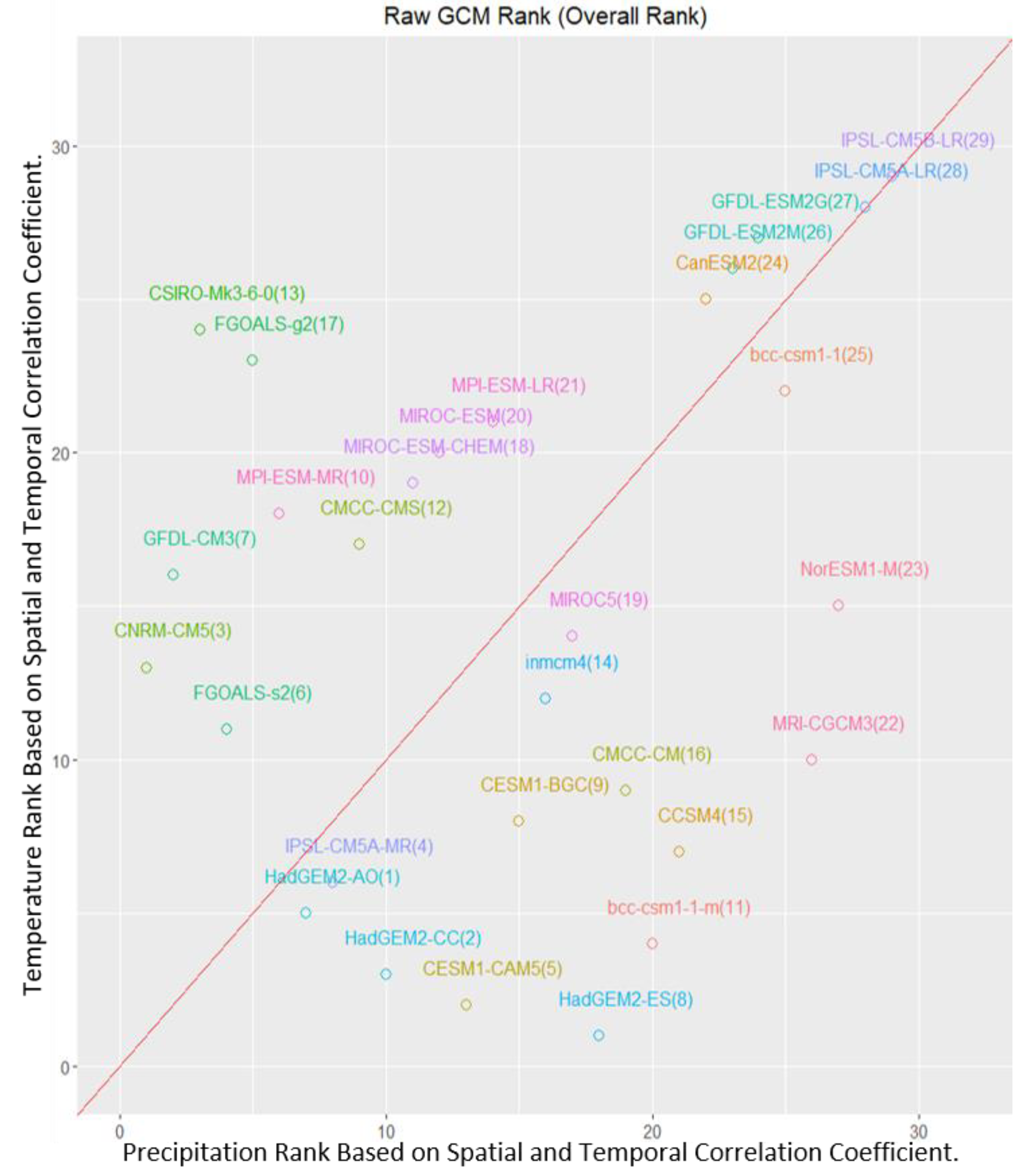
Twelve GCMs (Table 6) were selected for the study basin after raw GCM analysis (Figure 5) compared to the historical observation data (data period 1987–2016). With reference to the findings from several studies, multi-model ensemble (MME) accounted for the uncertainty of the single model [51,54], MME was prepared with an ensemble average of 12 best GCMs for the study area. The data were analyzed based on six scenarios, three each for RCP 4.5 and RCP 8.5 (Table 7).
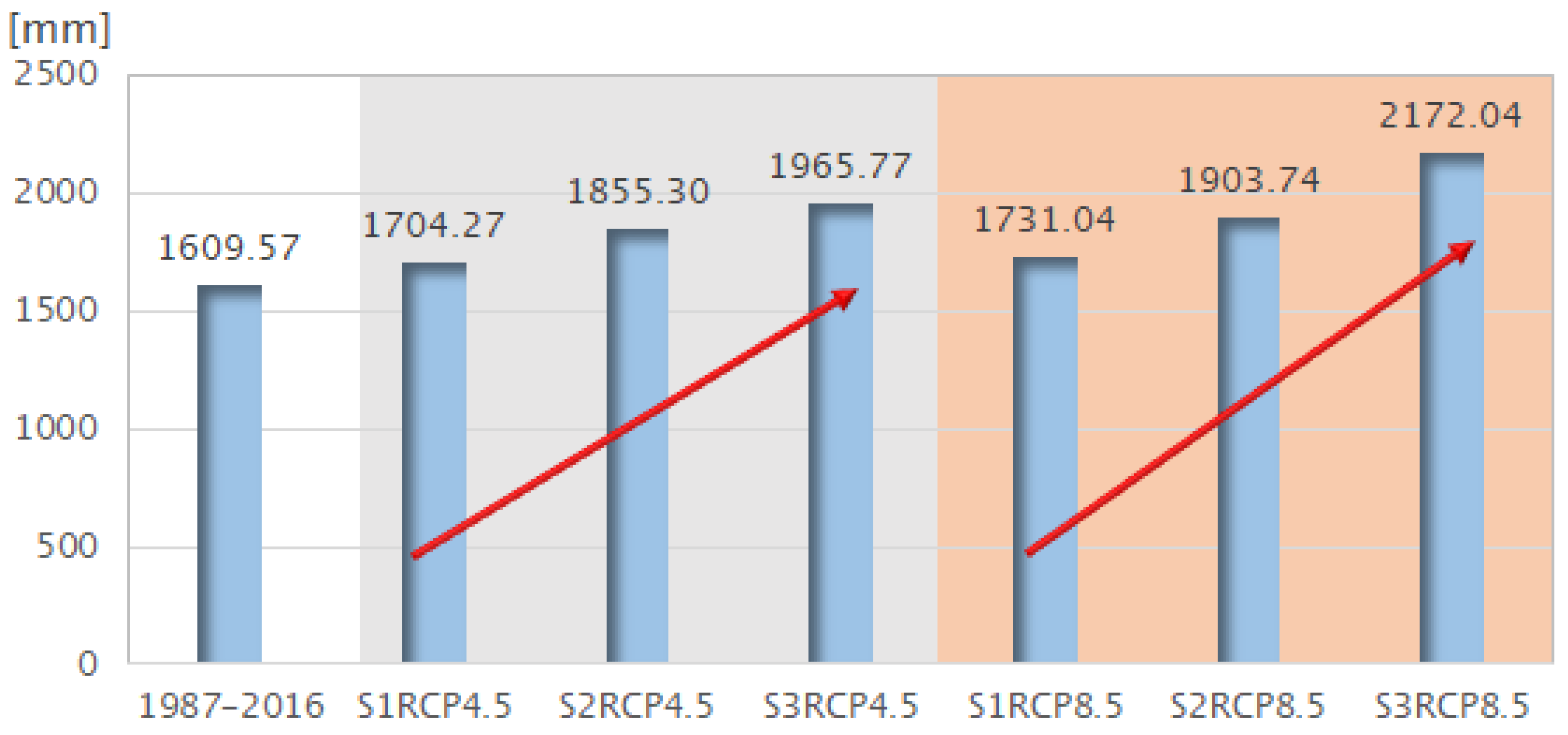
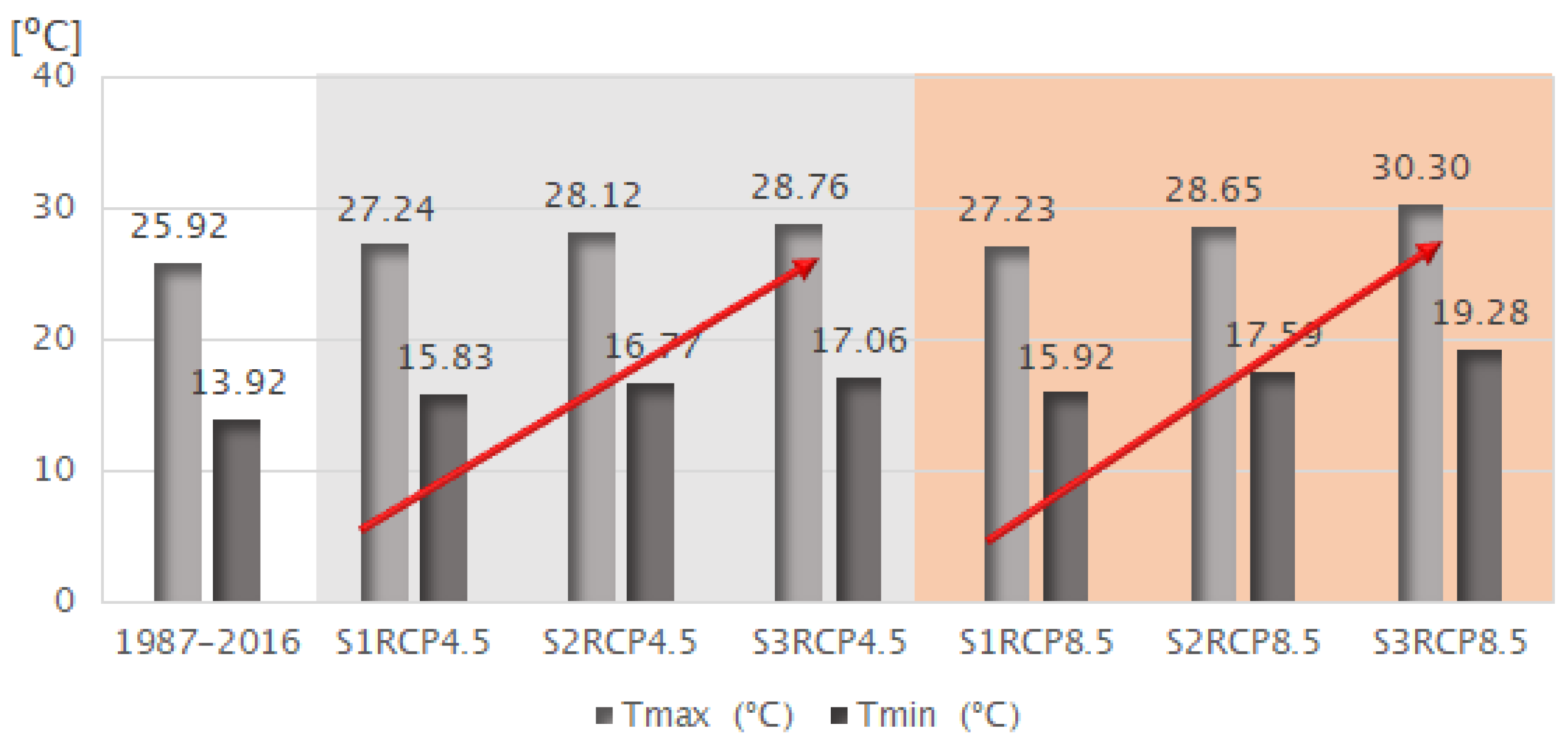
The patterns of two climate parameters (temperature and precipitation) were observed for the period 2010–2099 compared with the baseline historical period of 1987–2016 (Table 7). The average annual precipitation for the historical period was 1609.57 mm. It was observed that the average annual precipitation is expected to increase by 94.70 mm, 245.73 mm, and 356.20 mm in RCP 4.5 and 121.47 mm, 294.17 mm, and 562.47 mm under RCP 8.5 by the ends of 2030, 2060, and 2090, respectively (Figure 6). Likewise, the annual average maximum and minimum temperature for the baseline period (1987–2016) was 25.92 °C and 13.92 °C, respectively. Compared to the baseline period, the average maximum temperature (Tmax) is projected to increase by 1.32 °C, 2.20 °C, and 2.84 °C under RCP 4.5 and 1.31 °C, 2.73 °C, and 4.38 °C under RCP 8.5 by the ends of 2030, 2060, and 2090, respectively (Figure 7). The increment in the average minimum temperature (Tmin) is high for all scenarios compared to the maximum temperature. The average minimum temperature is projected to increase by 1.91 °C, 2.85 °C, and 3.14 °C under RCP 4.5 and 2.00 °C, 3.67 °C, and 5.36 °C under RCP 8.5 by the ends of 2030, 2060, and 2090, respectively, compared to the baseline period.
3.3. Impacts on Ecosystem Services (ES)
3.3.1. Water Yield
The average annual precipitation was 1879.53 mm and 1766.59 mm for the periods of 2000 and 2010, respectively. Comparing the two periods, the WY is observed to decrease by 106.592 MCM (million cubic meters) from 2000 to 2010. Figure 8 shows a raster map for the difference of WY between 2000 and 2010. In 2000, the total average annual WY was observed to be 3278.609 MCM and in 2010, WY was 3172.017 MCM. Performing a sub-basin-scale evaluation, WY was observed to have decreased in 2010 in all sub-basins except in sub-basin 2 (Table 8). As the computation of WY is a factor of evapotranspiration along with precipitation and LULC change, increment in the water yield in sub-basin 2 is attributable to an increase in the built-up area, which comes up with several other consequences like increased nitrogen load and reduced carbon storage.
The assessment of WY on climate scenarios based on the baseline land use of 2010 and the corresponding climate data obtained from MME of GCMs shows increased WY with an increased projection of precipitation in future scenarios (Table 9). Compared to 2010, the total WY of the basin is observed to decrease in S1Rcp4.5 and S1Rcp8.5. However, even with the baseline LULC of 2010, the total WY was observed to increase from period S1 to S2 to S3 under both RCP 4.5 and RCP 8.5 scenarios. The WY per ha is highest on sub-basin 5 and lowest on sub-basin 1 in 2010 but, in future scenarios, sub-basin 6 will have the highest WY and sub-basin 2 will have the lowest water yield per ha of land (Table 9). This provides a general estimate and trend of WY but as WY is a function of evapotranspiration, highly affected by LULC, projections based on future LULC scenarios can give a better estimate.
3.3.2. Soil Loss
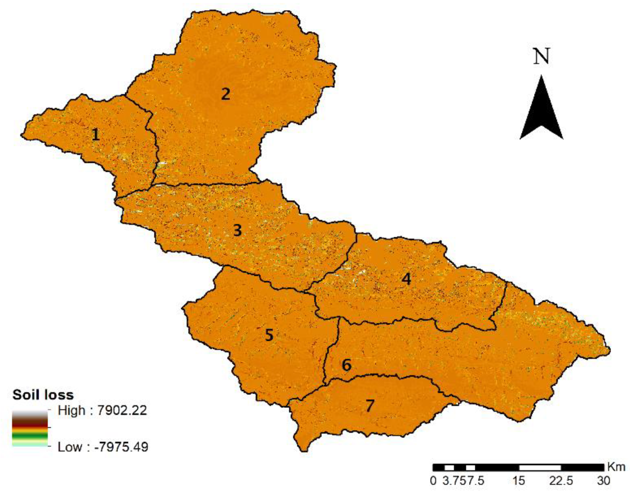
The annual average soil loss is reduced in 2010 (20.46 Mt/yr) compared to 2000 (21.38 Mt/yr) and is attributable to decreased annual average precipitation. Figure 9 shows a raster map for the difference of soil loss between 2000 and 2010. In 2000, agriculture accounted for the highest average rate of soil loss (198.40 t/yr/ha) whereas, in 2010, barren land was responsible for the highest soil loss (225.62 t/yr/ha) (Table 10). In both periods, the highest average rate of soil loss was as a result of agricultural land use causing 56.07% and 56.06% of total soil loss in 2000 and 2010, respectively.
The assessment of soil loss on future periods under RCP 4.5 and RCP 8.5 was computed with the baseline LULC map of 2010 and projected MME of climate data. The increment in precipitation will result in increased rainfall erosivity and, hence, soil loss is projected to increase in all consequent future scenarios. Soil loss increased by 1.53, 1.74, and 3.1 Mt/yr in S1, S2, and S3 periods, respectively, under the RCP 4.5 scenario. Likewise, under RCP 8.5, soil loss was projected to increase by 3.63, 4.23, and 6.59 Mt/yr in S1, S2, and S3 periods, respectively (Table 11).
3.3.3. Nitrogen Export
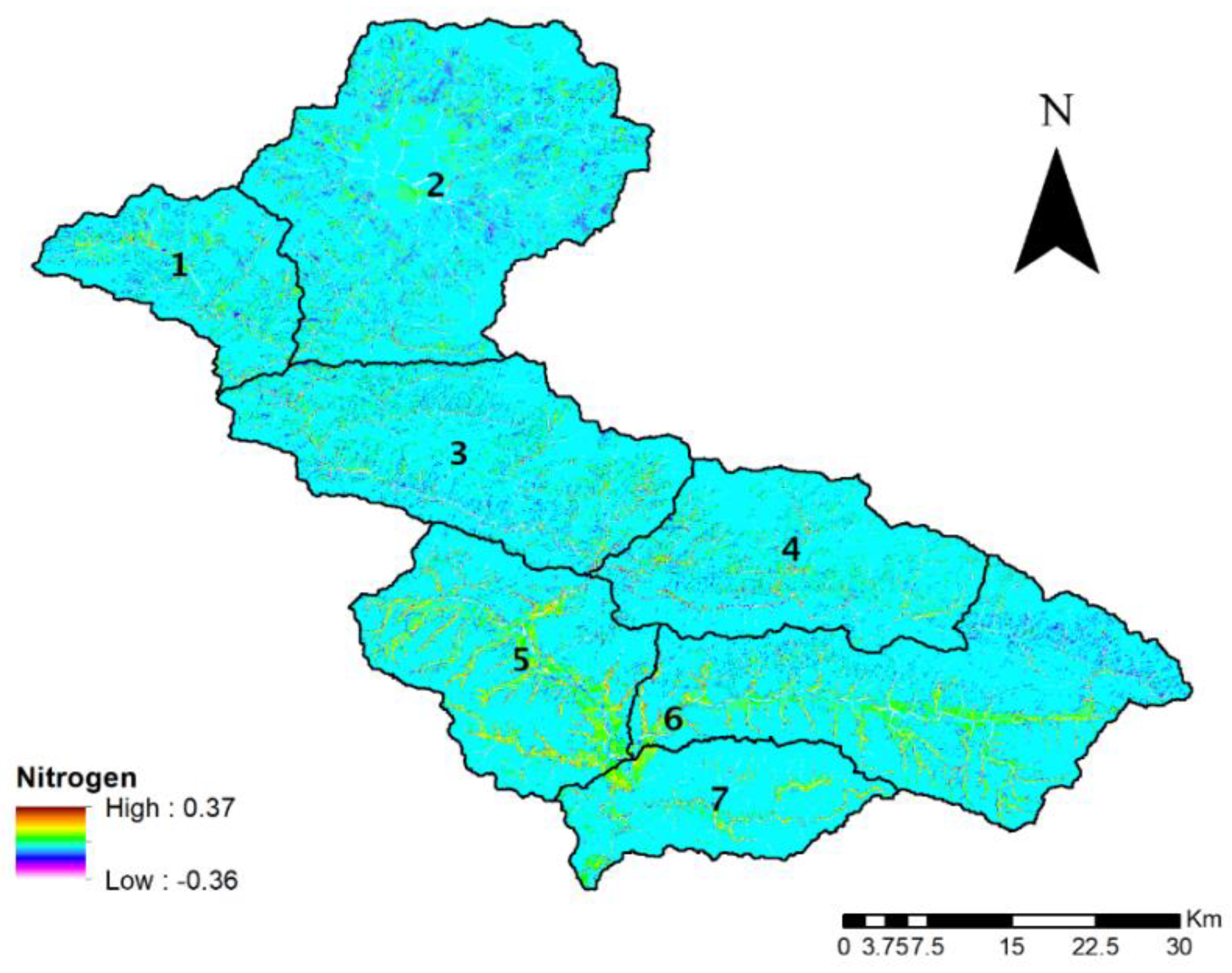
Nitrogen export from the various LULC types directly affects the watershed health, humans, and aquatic life processes. The comparative study (Table 12) of nitrogen export between LULC of 2000 and 2010 (Figure 10) showed that the total nitrogen export of the basin increased by 34,490.90 kg in 2010 compared to 2000. The sub-basin-scale evaluation shows that nitrogen export was the highest from sub-basin 2 in both periods. The assessment of nitrogen export on future scenarios with projected MME of climate data and the baseline LULC of 2010 did not show a precise pattern like other ES. The nitrogen export was determined based on LULC and associated loading rates. As the study was conducted on baseline land use of 2010, the comparative value of nitrogen export on climate scenarios was observed to be less than that of the 2010 case. The estimation with future land use scenarios can enhance the accuracy of estimation. However, in all cases (Table 13), nitrogen export was highest in sub-basin 2 and lowest in sub-basin 7 like in the baseline period of 2010.
3.3.4. Carbon Storage
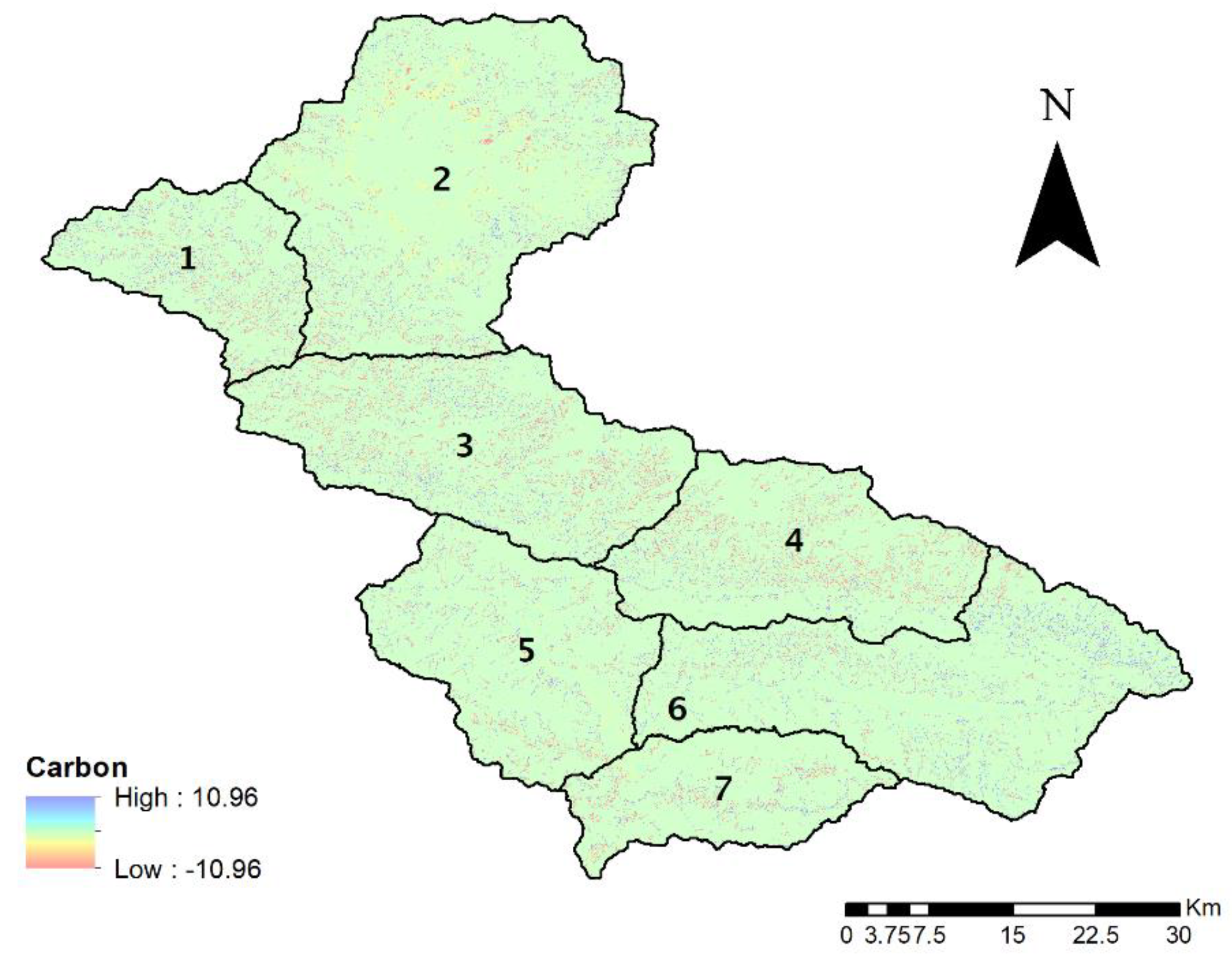
The total modeled carbon was reduced by 969,923.33 Mg from 2000 to 2010. The reduction in forest cover, shrubland, and grassland caused the overall reduction of carbon storage on the basin. Likewise, a sub-basin-scale evaluation of carbon storage shows that, in both periods, carbon storage per ha was the highest in sub-basin 7 and lowest in sub-basin 2 (Table 14). Figure 11 shows a raster file for the difference in carbon storage between 2000 and 2010. There were increased anthropogenic activities in sub-basin 2 which is mostly comprised of residential/built-up areas and agricultural areas of the basin. This represents the area with the lowest storage despite having the highest area. Likewise, comparing total carbon storage in 2000 and 2010, sub-basin 2 marks the highest loss with a 315,381.00 Mg reduction and sub-basin 6 has increased storage by 168,886.91 Mg.
4. Discussion
The global concern for the conservation and promotion of ES is rising along with an awareness that projected extreme events as a result of climate change will hamper the provision of services. Normally, ES are renewable if they can be managed sustainably but can be depleted or degraded if mismanaged. The future climate will continue to deliver ES; in some cases, ES are increased and, in some cases, decreased—mostly decreased compared to historical supply. Along with climate change, another important factor is LULC transformation, which alters the provision of ES. Thus, mapping and evaluation of ES are crucial for future land use plans and for strengthening the capability of various services and facilities, directly or indirectly associated with ES.
Provisioning services are often readily appreciated by the public as they have direct market values. However, other ES (regulating services, supporting services, and cultural services) are often not prioritized in decision making as these services do not hold immediate monetary value. To emphasize the significance of regulating services in the production and sustainability of other ES, we focused on four major regulating ES, namely, WY, soil loss, nitrogen export, and carbon storage. The provision of these services was compared on sub-basin scales and compared based on LULC data of two time periods, namely, 2000 and 2010. We also computed the ES provision on future climate scenarios with the baseline LULC data of 2010 and downscaled climate data for 2010–2099.
The LULC change analysis between the periods 2000 and 2010 shows that the conversion to built-up and agriculture areas from other LULC is significantly high on the Bagmati Basin. This is because of increased anthropogenic activities for food sustainability and economic upliftment. These conversions come at the huge cost of increased WY, soil loss, loss of carbon sink, and increased nitrogen export to water resources. Meantime, the concept of a Payments for Ecosystem Services (PES) scheme is being promoted in the basin with the realization of the need for ecosystem conservation [55]. This scheme has increased protected areas and community forests in the basin and has a twin objective of promoting ecosystem conservation and development earnings [55]. Likewise, climate projection shows increased precipitation and temperatures for the future period. The mean annual average precipitation in the case of 2010 was lower than that of 2000 and as WY and soil loss are highly affected by precipitation amount, its magnitude was decreased in 2010 compared to 2000. Though the overall WY was decreased in 2010 compared to 2000, the WY on sub-basin 2 increased. Sub-basin 2 faced a higher increment of built-up areas and, consequently, evaporative loss and water retention were reduced, causing an overall increase of WY. This phenomenon was also observed by another study [56] when computing the impacts of LULC on WY provision. The prediction of WY on future climate scenarios shows an overall increase in all sub-basins in consecutive periods S1 to S3 under both RCP 4.5 and RCP 8.5 scenarios (Table 9). Although precipitation determines the amount of water provided by nature, LULC plays a significant role in determining the amount of water that flows as runoff or is retained as storage [57]. Owing to this phenomenon, urbanization has induced frequent urban floods in Nepal and the lack of sufficient water retention structures has increased flood peaks and flood volumes.
In terms of ES, changes in WY caused by LULC changes have two major effects, namely, contribution to the water available for consumption and/or increased flood risks during storms [58]. Infrastructural capability for water collection, delivery, and treatment may work temporarily to counter increased WY. In the long term, however, management should consider human–nature interactions to avoid unintended environmental and socio-economic consequences which are caused as a result of rapid and large-scale development [58]. Several studies have recommended ecosystem-based “green” infrastructures such as wetlands, well-structured soils, and forest patches to enhance water storage and flood regulation [59]. The mapping of WY and its tendencies in future climate scenarios can hence provide an outline for such sustainable land use plans to mitigate flood risks and water scarcity problems.
Although soil loss due to erosion and sedimentation are natural processes in a healthy ecosystem, excess loss mainly due to changes in LULC is a threat to the security of water, food, and energy [60]. Soil loss is observed to be highest from agricultural land use in the study basin. Agriculture is the major activity sustaining the economy of Nepal. Thus, the traditional agricultural system demands improved methods to sustain topsoil-containing organic matter and essential plant nutrients that are otherwise removed from the soil during erosion. Likewise, the predicted increment of soil loss in the future climate scenarios also indicates the necessity for improved farm management practices that incorporate the management of increased WY. In addition to the stress on food production, soil erosion also reduces water and nutrient retention, biodiversity, and water resources/downstream power generation [61]. Therefore, for sustainable management of soils and related services, spatial mapping of soil erosion on different land use and future scenarios can provide guidelines and mark areas for immediate actions to mitigate the loss.
The loss of carbon storage is another significant phenomenon observed in the study basin with a reduction in forest areas and increases in agricultural and built-up areas. Terrestrial-based carbon storage and sequestration are directly affected by LULC. The concentrated anthropogenic activities on the upper part of the basin, especially in sub-basin 2, contribute to the lowest carbon storage and highest nitrogen export per ha of land in this sub-basin. Most developing nations have serious problems with the degradation of forests and soils which have crucial implications for changing the global C pools [62]. The information on carbon storage and fluctuations can help land managers to choose among sites for protection, harvest, or development. Furthermore, these maps can support multiple decisions by governments, NGOs, and stakeholders to offer incentives to landowners in exchange for forest conservation. Sub-classification of land use and consideration of altitudinal variation in various carbon pools produces more accurate results. Poudel et al. [63] have found higher carbon stocks at the higher altitudinal gradient in the study conducted in the Panchase Conservation Area in Nepal. The study indicated that due to human disturbance, carbon stocks were low at low altitude. Temperature and precipitation also have significant effects on the carbon pool of various biomass [64]. Thus, a detailed study with climate and elevation variation helps to produce an accurate estimate of carbon value.
Similarly, with increased agricultural activities, and reduced vegetation covers, nutrient retention diminishes and, hence, the amount of nitrogen entering the river network/water resources increases. This severely increases water contamination, thereby affecting human and aquatic health. Additionally, because of increased WY in future climate scenarios, nitrogen export is expected to increase in all sub-basins. In this scenario, spatial information on nutrient export and areas with the highest filtration can help land use planners to integrate the contribution of ecosystems in order to mitigate water pollution.
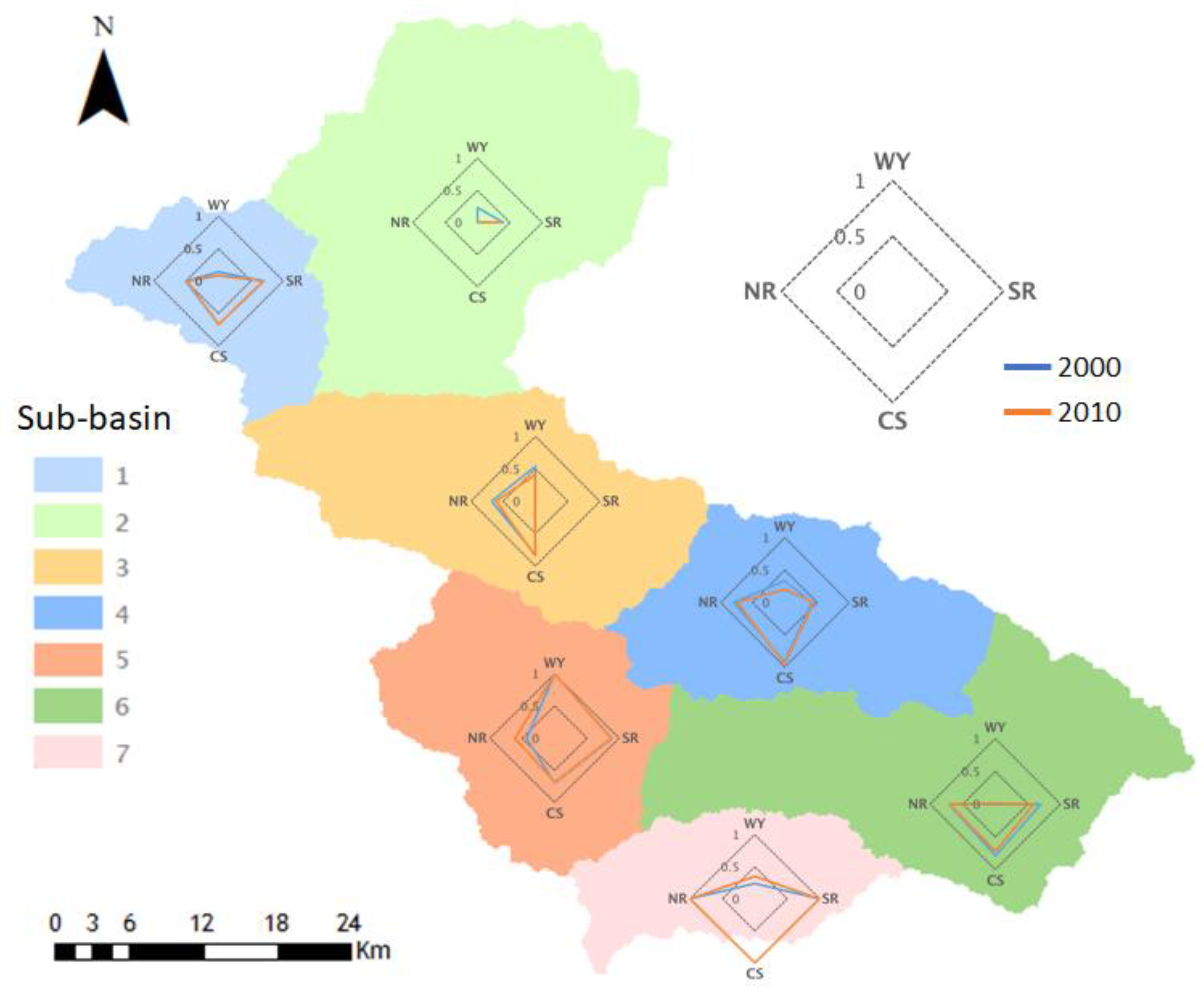
To understand the temporal change of ecosystem services in 2000 and 2010, the minimum value was set to 0 and the maximum value was set to 1 for each ecosystem service in two periods. This shows a comparative provision of ES in all sub-basins in the 2000 and 2010 periods which depicted that sub-basin 2 had the lowest combined ES provision in both 2000 and 2010 (Figure 12). Thus, this indicates the need for urgent policies in order to restore the services and to promote its sustainability. Likewise, the computation of ES with the projection of climate data in the 2010–2099 period shows increased WY, soil loss, and nitrogen export from the study area. The case of sub-basin 2, especially of the Kathmandu Valley area, can be referenced for the planning of other emerging cities. As Nepal is prioritizing decentralization and focusing on the development of many other smart cities on the outskirts of the Kathmandu Valley and other parts of the country, studies like this can present risk analyses and help decision making that prioritizes the conservation of ES for the optimum utilization and preservation of natural capital.
5. Limitations of the Study
The InVEST tools used for the evaluation of ES have their own modeling limitations. The InVEST WY Model is based on annual averages and neglects the extremes and the spatial distribution of LULC. The InVEST Carbon Storage Model assumes that each LULC is at the fixed carbon storage level and the fluctuation on carbon storage is only due to a change in LULC from one type to another. Due to data unavailability in the study area, tabular values were obtained from the InVEST manual. The study used reference data for various LULC types from InVEST user guidelines and the variation in the amount of carbon storage in different carbon pools due to elevation have not been acknowledged in the study at this stage. In addition, for climate data, uncertainties remain from climate change data itself and from the selected methods of downscaling and bias correction. Nevertheless, careful attention was given to the preparation of data and modeling. Despite the model and data limitations, the results from the study provide an overview of a general tendency of the provision of ES, including fluctuations with a change in climate and LULC. It is, thus, expected to help in decision making and scenario analysis. The results of this study could be improved if ground observation data are available for the accurate analysis of InVEST models.
6. Conclusions
This study attempted to evaluate ES and their fluctuations with LULC and climate change on the Bagmati Basin of Nepal. The study first assessed ES based on the 2000 and 2010 LULC map and then with the baseline LULC map of 2010 and projected climate data from the MME of 12 GCMs, ES provision on the future period was estimated. The overall provision of combined ES on sub-basin 2 was lowest in 2000, 2010, and on all future climate scenarios. In addition, the provision of ES was observed to be decreasing in all other sub-basins. Outcomes like increased WY, reduced carbon storage, increased nitrogen export, and soil loss suggest that immediate actions are required from policy makers for the sustainable management of natural capital. The ES are interrelated and the absence of adequate designs to sustain one can hamper other provisions as well. The availability of spatially explicit information on ecosystems and their interrelated services serves for the prioritization of ES into policy and decision making. The maps produced as an outcome of this study can help land use planners, government organizations, and concerned stakeholders to recognize areas where the ecosystems are produced and help in the decision making for low impact development maintaining ecological balance and economic goals. Further studies on national scale future LULC scenarios could estimate accurate ES provisions integrating national priorities.
Supplementary Materials
The following are available online at https://www.mdpi.com/2071-1050/12/19/8186/s1, Table S1: list of stations with rainfall and temperature data along with their location and data period. The data has been duly collected from Department of Hydrology and Meteorology (DHM) Nepal.
Author Contributions
Conceptualization, Y.J. and S.B.; methodology, S.B. and S.L.; formal analysis, S.B. and S.L.; writing—original draft preparation, S.B.; writing—review and editing, Y.S. and Y.J.; project administration, Y.J.; funding acquisition, Y.S. All authors have read and agreed to the published version of the manuscript.
Funding
This subject is supported by the Korea Ministry of Environment as “The SS (Surface Soil conservation and management) projects; 2019002820002”.
Acknowledgments
The authors send special thanks to the Korean Environment Institute (KEI) for their data collection efforts.
Conflicts of Interest
The authors declare no conflict of interest.
References
- Vihervaara, P.; Rönkä, M.; Walls, M. Trends in ecosystem service research: Early steps and current drivers. AMBIO 2010, 39, 314–324. [Google Scholar] [CrossRef] [PubMed]
- Millennium Ecosystem Assessment. Ecosystems and Human Well-Being: Biodiversity Synthesis; Island Press: Washington, DC, USA, 2005. [Google Scholar]
- Cardinale, B.J.; Duffy, J.E.; Gonzalez, A.; Hooper, D.U.; Perrings, C.; Venail, P.; Narwani, A.; Mace, G.M.; Tilman, D.; Wardle, D.A.; et al. Biodiversity loss and its impact on humanity. Nature 2012, 486, 59–67. [Google Scholar] [CrossRef] [PubMed]
- Foley, J.A.; DeFries, R.; Asner, G.P.; Barford, C.; Bonan, G.; Carpenter, S.R.; Chapin, F.S.; Coe, M.T.; Daily, G.C.; Gibbs, H.K.; et al. Global consequences of land use. Science 2005, 309, 570–574. [Google Scholar] [CrossRef] [Green Version]
- Marx, A.; Erhard, M.; Thober, S.; Kumar, R.; Schafer, D.; Samaniego, L.; Zink, M. Climate Change as Driver for Ecosystem Services Risk and Opportunities. In Atlas of Ecosystem Services; Springer: Cham, Switzerland, 2019; pp. 173–178. [Google Scholar]
- IPCC (Intergovernmental Panel on Climate Change). Climate Change 2013: The Physical Science Basis. Contribution of Working Group I to the Fifth Assessment Report of the Intergovernmental Panel on Climate Change; Stocker, T.F., Qin, D., Plattner, G.K., Tignor, M., Allen, S.K., Boschung, J., Nauels, A., Xia, Y., Bex, V., Midgley, P.M., Eds.; Cambridge University Press: Cambridge, UK; New York, NY, USA, 2013. [Google Scholar]
- IPCC (Intergovernmental Panel on Climate Change). Climate Change 2014: Impacts, Adaptation, and Vulnerability. Part A: Global and Sectoral Aspects. Contribution of Working Group II to the Fifth Assessment Report of the Intergovernmental Panel on Climate Change; Field, C.B., Barros, V.R., Dokken, D.J., Mach, K.J., Mastrandrea, M.D., Bilir, T.E., Chatterjee, M., Ebi, K.L., Estrada, Y.O., Genova, R.C., et al., Eds.; Cambridge University Press: Cambridge, UK; New York, NY, USA, 2014. [Google Scholar]
- Srinivasan, U.T. Economics of climate change: Risk and responsibility by world region. Clim. Policy 2010, 10, 298–316. [Google Scholar] [CrossRef]
- Mandle, L.; Wolny, S.; Bhagabati, N.; Helsingen, H.; Hamel, P.; Bartlett, R.; Dixon, A.; Horton, R.; Lesk, C.; Manley, D.; et al. Assessing ecosystem service provision under climate change to support conservation and development planning in Myanmar. PLoS ONE 2017, 12, e0184951. [Google Scholar] [CrossRef] [Green Version]
- Lambin, E.F.; Geist, H.J.; Ellis, E. Causes of Land-Use and Land-Cover Change. In Environmental Information Coalition, National Council for Science and the Environment; Cleveland, C.J., Ed.; Encyclopedia of Earth: Washington, DC, USA, 2007. [Google Scholar]
- Ramankutty, N.; Graumlich, L.; Achard, F.; Alves, D.; Chhabra, A.; DeFries, R.S.; Foley, J.; Geist, H.; Houghton, R.A.; Goldewijk, K.K.; et al. Land-Use and Land-Cover Change: Local Processes with Global Impacts; Springer: Berlin/Heidelberg, Germany, 2006; pp. 1–8. [Google Scholar]
- Yuan, F.; Sawaya, K.; Loeffelholz, B.; Bauer, M. Land cover classification and change analysis of the Twin cities (Minnesota). Metropolitan Area by multitemporal Landsat Remote Sensing. Remote Sens. Environ. 2005, 98, 317–328. [Google Scholar] [CrossRef]
- Juanita, A.D.; Ignacio, P.; Jorgelina, G.A.; Cecilia, A.S.; Carlos, M.; Francisco, N. Assessing the effects of past and future land cover changes in ecosystem services, disservices and biodiversity: A case study in Barranquilla Metropolitan Area (BMA), Colombia. Ecosyst. Serv. 2019, 37, 100915. [Google Scholar] [CrossRef]
- Central Bureau of statistics (CBS). Nepal, National Population and Housing Census 2011; Government of Nepal, National planning Commission Secretariat: Kathmandu, Nepal, 2012.
- UNDESA (United Nations, Department of Economic and Social Affairs). World Urbanization Prospects. The 2014 Revision; UNDESA: New York, NY, USA, 2015. [Google Scholar]
- Paudel, A. Environmental management of the Bagmati River Basin. In UNEP EIA Training Resource Manual, Case Studies from Developing Countries; McCabe, M., Sadler, B., Eds.; UNEP: Nairobi, Kenya, 2002; pp. 269–279. Available online: https://www.iaia.org/pdf/case-studies/BasmatiRiverBasin.pdf (accessed on 10 December 2019).
- Asian Development Bank. Concept Paper, Nepal: Bagmati River Basin Improvement Project. Project Number: 43448. January 2012. Available online: https://www.adb.org/sites/default/files/project-document/74141/43448-013-nep-cp.pdf (accessed on 25 November 2019).
- Thapa, I.; Butchart, H.M.S.; Gurung, H.; Statterfield, A.J.; Thomas, D.H.L.; Birch, J.C. Using information on ecosystem services in Nepal to inform biodiversity conservation and local to national decision-making. Oryx 2016, 50, 147–155. [Google Scholar] [CrossRef] [Green Version]
- IUCN. Payment for Ecosystem Services in Nepal. Prospect, Practice and Process; IUCN Nepal: Kupondole, Nepal, 2013. [Google Scholar]
- Rai, R.; Zhang, Y.; Paudel, B.; Acharya, B.; Basnet, L. Land Use and Land Cover Dynamics and Assessing the Ecosystem Service Values in the Trans-Boundary Gandaki River Basin, Central Himalayas. Sustainability 2018, 10, 3052. [Google Scholar] [CrossRef] [Green Version]
- Rimal, B.; Sharma, R.; Kunwar, R.; Keshtkar, H.; Stork, N.E.; Rijal, S.; Rahman, S.A.; Baral, H. Effects of land use and land cover change on ecosystem services in the Koshi River Basin, Eastern Nepal. Ecosyst. Serv. 2019, 38, 100963. [Google Scholar] [CrossRef]
- Chettri, N.; Aryal, K.; Kandel, P.; Karki, S.; Uddin, K. Ecosystem Services Assessment: A Framework for Himalica; International Centre for Integrated Mountain Development: Kathmandu, Nepal, 2014. [Google Scholar]
- Thakur, J.K.; Neupane, M.; Mohanan, A.A. Water Poverty in Upper Bagmati River Basin in Nepal. Water Sci. 2017, 31, 93–108. [Google Scholar] [CrossRef] [Green Version]
- Khanal, P.R.; Lee, S.; Khanel, S.R.; Khan, S.P.; Lee, Y.S. Spatial–temporal variation and comparative assessment of water qualities of urban river system: A case study of the river Bagmati (Nepal). Environ. Monit. Assess. 2007, 129, 433–459. [Google Scholar]
- Bhattarai, R. Sediment transport modelling using GIS in Bagmati basin, Nepal. Sedim. Transp. Process. Model. Appl. 2013, 13, 77. [Google Scholar] [CrossRef]
- Schirpke, U.; Candiago, S.; Egarter Vigl, L.; Jäger, H.; Labadini, A.; Marsoner, T.; Meisch, C.; Tasser, E.; Tappeiner, U. Integrating supply, flow and demand to enhance the understanding of interactions among multiple ecosystem services. Sci. Total Environ. 2019, 651, 928–941. [Google Scholar] [CrossRef]
- Sharp, R.; Tallis, H.T.; Ricketts, T.; Guerry, A.D.; Wood, S.A.; Chaplin-Kramer, R.; Nelson, E.; Ennaanay, D.; Wolny, S.; Olwero, N.; et al. InVEST 3.6.0 User’s Guide; The Natural Capital Project, Stanford University: Stanford, CA, USA, 2018. [Google Scholar]
- Renard, K.G.; Foster, G.R.; Weesies, G.A.; McCool, D.K.; Yoder, D.C. Predicting Soil Erosion by Water: A Guide to Conservation Planning with the Revised Universal Soil Loss Equation (RUSLE); US Government Printing Office: Washington, DC, USA, 1997.
- Bagmati Basin River Improvement Project (BRBIP). Available online: Brbip.gov.np (accessed on 18 November 2019).
- Mishra, B.; Herath, S. Assessment of Future Floods in the Bagmati River Basin of Nepal Using Bias-Corrected Daily GCM Precipitation Data. J. Hydrol. Eng. 2015, 20, 05014027. [Google Scholar] [CrossRef]
- Uddin, K.; Shrestha, H.L.; Murthy, M.S.R.; Bajracharya, B.; Shrestha, B.; Gilani, H.; Pradhan, S.; Dangol, B. Development of 2010 national land cover database for the Nepal. J. Environ. Manag. 2014, 148, 82–90. [Google Scholar] [CrossRef] [PubMed]
- Earth Data GES DISC. Atmospheric Composition, Water and Energy Cycles and Climate Variability. Available online: https://disc.gsfc.nasa.gov/datasets?keywords=%22MERRA2%22&page=1&source=Models%2FAnalyses%20MERRA-2 (accessed on 24 March 2019).
- Cong, W.; Sun, X.; Guo, H.; Shan, R. Comparison of the SWAT and InVEST models to determine hydrological ecosystem service spatial patterns, priorities and trade-offs in a complex basin. Ecol. Indic. 2020, 112, 106089. [Google Scholar] [CrossRef]
- Fu, B.P. On the calculation of the evaporation from land surface. Chin. J. Atmos. Sci. 1981, 5, 23–31. [Google Scholar]
- Zhang, L.; Hickel, K.; Dawes, W.R.; Chiew, F.H.S.; Western, A.W.; Briggs, P.R. A rational function approach for estimating mean annual evapotranspiration. Water Resour. Res. 2004. [Google Scholar] [CrossRef]
- Donohue, R.J.; Roderick, M.L.; McVicar, T.R. Roots, storms and soil pores: Incorporating key ecohydrological processes into Budyko’s hydrological model. J. Hydrol. 2012, 436, 35–50. [Google Scholar] [CrossRef]
- Hargreaves, G.H.; Samani, Z.A. Reference Crop Evapotranspiration from Temperature. Appl. Eng. Agric. 1985, 1, 96–99. [Google Scholar] [CrossRef]
- Chen, S.X.; Xie, L.; Zhang, J.C. Root system distribution characteristics of main vegetation types in Anji County of Zhejiang Provence. Subtrop. Soil Water Conserv. 2008, 20, 1–4. [Google Scholar]
- Allen, R.G.; Pereira, L.S.; Raes, D.; Smith, M. Crop Evapotranspiration. Guidelines for Computing Crop Water Requirements; FAO Irrigation and Drainage Paper 56; Food and Agriculture Organization of the United Nations: Rome, Italy, 1998. [Google Scholar]
- Lu, H.; Prosser, I.; Moran, C.; Gallant, J.; Priestley, G.; Stevenson, J.G. Predicting sheetwash and rill erosion over the Australian continent. Aust. J. Soil Res. 2003, 41, 1037–1062. [Google Scholar] [CrossRef]
- Singh, G.; Chandra, S.; Babu, R. Soil Loss and Prediction Research in India. Bulletin No. T-12/D9; Central Soil and Water Conservation Research Training Institute: Dehra Dun, India, 1981.
- Gardner, R.A.M.; Gerrard, A.J. Runoff and soil erosion on cultivated rain fed terraces in the Middle Hills of Nepal. Appl. Geogr. 2003, 23, 23–45. [Google Scholar] [CrossRef]
- Jain, S.K.; Kumar, S.; Varghese, J. Estimation of Soil Erosion for a Himalayan Watershed Using GIS Technique. Water Resour. Manag. 2001, 15, 41–54. [Google Scholar] [CrossRef]
- Vopravil, J.; Janeček, M.; Tippl, M. Revised soil erodibility K-factor for soils in the Czech Republic. Soil Water Res. 2007, 2, 1–9. [Google Scholar] [CrossRef] [Green Version]
- Wischmeier, W.H.; Smith, D.D. Predicting Rainfall Erosion Losses: A Guide to Conservation Planting. United States Department of Agriculture; Agriculture Handbook: No.537; United States Department of Agriculture: Washington, DC, USA, 1978.
- McCool, D.K.; Brown, L.C.; Foster, G.R.; Mutchler, C.K.; Meyer, L.D. Revised slope length factor for the universal soil loss equation. T. ASAE 1989, 30, 1387–1396. [Google Scholar] [CrossRef]
- Jha, R. Potential erosion map for Bagmati basin using GRASS GIS. In Proceedings of the Open Source GIS-GRASS Users’ Conference, Trento, Italy, 11–13 September 2002. [Google Scholar]
- Line, D.E.; White, N.M.; Osmond, D.L.; Jennings, G.D.; Mojonnier, C.B. Pollutant export from various land uses in the upper Neuse river basin. Water Environ. Res. 2002, 74, 100–108. [Google Scholar] [CrossRef]
- Qiu, J.; Turner, M.G. Spatial interactions among ecosystem services in an urbanizing agricultural watershed. Proc. Natl. Acad. Sci. USA 2013, 110, 12149–12154. [Google Scholar] [CrossRef] [Green Version]
- Gurung, K.; Yang, J.; Fang, L. Assessing Ecosystem Services from the Forestry-Based Reclamation of Surface Mined Areas in the North Fork of the Kentucky River Watershed. Forests 2018, 9, 652. [Google Scholar] [CrossRef] [Green Version]
- Cho, J.; Ko, G.; Kim, K.; Oh, C. Climate Change Impacts on Agricultural Drought with Consideration of Uncertainty in CMIP5 Scenarios. Irrig. Drain. 2016, 65, 7–15. [Google Scholar] [CrossRef]
- Van Vuuren, D.P.; Edmonds, J.; Kainuma, M.; Riahi, K.; Thomson, A.; Hibbard, K.; Hurtt, G.; Kram, T.; Krey, V.; Lamarque, J.F.; et al. The representative concentration pathways: An overview. Clim. Chang. 2011, 109, 5–31. [Google Scholar] [CrossRef]
- APCC Integrated Modelling Solution. Available online: aims.apcc21.org (accessed on 15 October 2018).
- Harding, R.; Reynard, N.; Kay, A.L. Current understanding of climate change impacts on extreme events. Hydrometeorological Hazards. Interfacing Sci. Policy 2014. [Google Scholar] [CrossRef]
- PES Policies. ICIMOD. In Proceedings of the National Workshop on Payment for Ecosystem Services: Opportunities and Challenges in Nepal, Kathmandu, Nepal, 18–19 September 2014. [Google Scholar]
- Li, S.; Yang, H.; Lacayo, M.; Liu, J.; Guangchun, L. Impacts of Land-Use and Land-Cover Changes on Water Yield: A Case Study in Jing-Jin-Ji, China. Sustainability 2018, 1, 960. [Google Scholar] [CrossRef] [Green Version]
- Brauman, K.A.; Daily, G.C.; Duarte, T.K.E.; Mooney, H.A. The nature and value of ecosystem services: An overview highlighting hydrologic services. Annu. Rev. Environ. Resour. 2007, 32, 67–98. [Google Scholar] [CrossRef]
- Liu, J.; Yang, W. Water sustainability for China and beyond. Science 2012, 337, 649–650. [Google Scholar] [CrossRef]
- Palmer, M.A.; Liu, J.; Matthews, J.H.; Mumba, M.; D’odorico, P. Manage water in a green way. Science 2015, 349, 584–585. [Google Scholar] [CrossRef] [Green Version]
- Blum, W.E.H. Soil and land resources for agricultural production: General trends and future scenarios: A worldwide perspective. Int. Soil Water Conserv. Res. 2013, 1, 1–14. [Google Scholar] [CrossRef] [Green Version]
- Pimentel, D.; Burgess, M. Soil erosion threatens food production. Agriculture 2013, 3, 443–463. [Google Scholar] [CrossRef] [Green Version]
- Lal, H.S.; Bajracharya, R.M.; Sitaula, B.K. Forest and Soil Carbon Stocks, Pools and Dynamics and Potential Climate Change Mitigation in Nepal. J. Environ. Sci. Eng. 2012, 1, 800–811. [Google Scholar]
- Poudel, A.; Sasaki, N.; Abe, I. Assessment of carbon stocks in oak forests along the altitudinal gradient: A case study in the Panchase Conservation Area in Nepal. Glob. Ecol. Conserv. 2020, 23, e01171. [Google Scholar] [CrossRef]
- Wang, G.; Ran, F.; Chang, R.; Yang, Y.; Luo, J.; Fan, J. Variations in the live biomass and carbon pools of Abies georgei along an elevation gradient on the Tibetan Plateau, China. Forest Ecol. Manag. 2014, 329, 255–263. [Google Scholar] [CrossRef]
Figure 1.
River basin and elevation map of Nepal.

Figure 2.
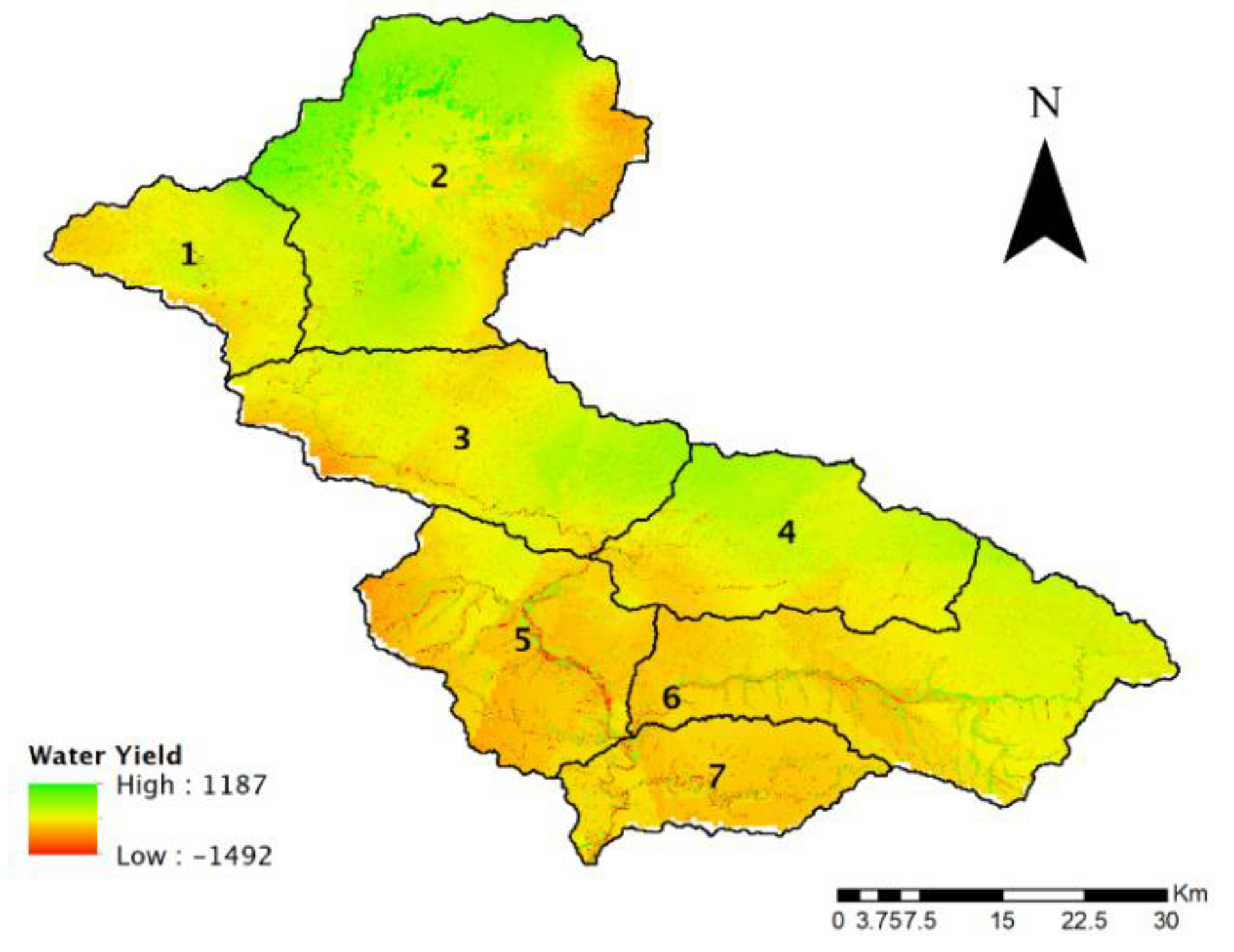
Sub-basins of the Bagmati Basin.

Figure 3.
Location of meteorological stations (rainfall data) with data from 1996–2015.

Figure 4.
Global temperature projections for various RCP scenarios Adapted from Intergovernmental Panel on Climate Change (IPCC) Fifth Assessment Report, 2013.
Figure 4.
Global temperature projections for various RCP scenarios Adapted from Intergovernmental Panel on Climate Change (IPCC) Fifth Assessment Report, 2013.

Figure 5.
Overall rank of used Coupled Model Intercomparison Project 5 (CMIP5) global climate model (GCM) for Nepal.
Figure 5.
Overall rank of used Coupled Model Intercomparison Project 5 (CMIP5) global climate model (GCM) for Nepal.

Figure 6.
Precipitation projection for future climate scenarios.

Figure 7.
Temperature projection for future climate scenarios.

Figure 8.
2000 and 2010 water yield (mm) difference map.

Figure 9.
2000 and 2010 soil loss (t/ha/yr) difference map.

Figure 10.
2000 and 2010 nitrogen export difference map (kg/pixel).

Figure 11.
2000 and 2010 carbon storage difference map (Mg/Pixel).

Figure 12.
Relative comparison of ES in 2000 and 2010.


Table 1.
Data description for InVEST Water Yield Model.
| SN | Data | Format | Data Source |
|---|---|---|---|
| 1 | Annual mean precipitation | Raster map | DHM * |
| 2 | Annual reference evapotranspiration | Raster map | Temperature data from DHM |
| 3 | Land use and land cover (LULC) | Raster map | ICIMOD ** Nepal |
| 4 | Soil depth | Raster map | SOTER *** database |
| 5 | Plant-available water content (PAWC) | Raster map | SOTER database |
| 6 | Basin and sub-basin | Shapefiles | ArcGIS |
| 7 | Biophysical table | Excel CSV table | Published literature |
SN—Serial Number. * DHM, Department of Hydrology and Meteorology. ** ICIMOD, International Centre for Integrated Mountain Development. *** SOTER, Soil and Terrain Database.
Table 2.
Biophysical attributes used for InVEST model.
| LULC | ||||||||
|---|---|---|---|---|---|---|---|---|
| Biophysical Attribute | Forest | Shrubland | Grassland | Agriculture Land | Barren Area | Water Body | Built-Up Area | Related Model |
| Land use code | 1 | 2 | 3 | 4 | 5 | 6 | 8 | Water Yield |
| Kc | 1 | 0.398 | 0.65 | 0.65 | 0.5 | 1 | 0.3 | |
| Root_depth | 7000 | 2000 | 2000 | 1500 | 500 | 0 | 0 | |
| LULC_veg | 1 | 1 | 1 | 1 | 0.001 | 0.001 | 0.001 | |
| Aboveground biomass | 90 | 8 | 6 | 3 | 0 | 0 | 0 | Carbon Storage |
| Belowground biomass | 60 | 8 | 6 | 2 | 0 | 0 | 0 | |
| Soil organic matter | 95 | 25 | 20 | 8 | 0 | 0 | 0 | |
| Dead organic matter | 29 | 3 | 2 | 1 | 0 | 0 | 0 | |
| Load_n | 1.8 | 2 | 4 | 11 | 4 | 0.001 | 7.25 | Nutrient Delivery |
| Eff_n | 0.8 | 0.4 | 0.5 | 0.25 | 0.05 | 0.05 | 0.05 | |
Kc = plant evapotranspiration coefficient. Root_depth = maximum root depth measured for vegetated LULC (mm). Load_n = nutrient loading for each land use measured in kg/ha/year. Eff_n = nutrient retention efficiency for each LULC class (floating point value, 0–1).
Table 3.
Overview of representative concentration pathways in IPCC AR5.
| Name | Radiative Forcing | CO2 Concentration (ppm) | Pathways |
|---|---|---|---|
| RCP 2.6 | Peak in radiative forcing at ~3 W/m2 before 2100 and decline | Peak at 490 before 2100 and then decline | Peak and decline |
| RCP 4.5 | 4.5 W/m2 at stabilization after 2100 | ~650 (at stabilization after 2100) | Stabilization without overshoot |
| RCP 6 | 6 W/m2 at stabilization after 2100 | ~850 (at stabilization after 2100) | Stabilization without overshoot |
| RCP 8.5 | >8.5 W/m2 in 2100 | >1370 CO2 equivalent in 2100 | Rising |
Source: Van Vuuren et al. [52].
Table 4.
Change in LULC between 2000 and 2010.
| LULC CLASS | LULC 2000 (ha) | LULC 2010 (ha) | Change | Percent Change (%) |
|---|---|---|---|---|
| Forest | 181,246.64 | 177,803.92 | −3442.72 | −1.90 |
| Shrubland | 2025.96 | 662.92 | −1363.04 | −67.28 |
| Grassland | 11,414.60 | 5402.48 | −6012.12 | −52.67 |
| Agriculture area | 60,545.56 | 69,777.56 | 9232.00 | 15.25 |
| Barren area | 7655.64 | 5003.60 | −2652.04 | −34.64 |
| Water body | 884.20 | 1034.84 | 150.64 | 17.04 |
| Built-up area | 13,124.52 | 17,211.80 | 4087.28 | 31.14 |
| Total | 276,897.12 | 276,897.12 |
Table 5.
Conversion of LULC in 2000 and 2010 (in ha).
| 2000 LULC | |||||||||
|---|---|---|---|---|---|---|---|---|---|
| 2010 LULC | LULC | Forest | Shrubland | Grassland | Agriculture | Barren | Water | Built-up | Total |
| Forest | 171,000.16 | 106.48 | 283.76 | 9362.92 | 95.24 | 89.2 | 308.88 | 181,246.64 | |
| Shrubland | 551 | 473.92 | 241.2 | 674.52 | 42.16 | 34.56 | 8.6 | 2025.96 | |
| Grassland | 886.04 | 47.84 | 1963.28 | 7555.8 | 543.72 | 156.12 | 261.8 | 11,414.6 | |
| Agriculture | 5202.24 | 14.88 | 2653.44 | 48,755.88 | 391.12 | 147.04 | 3380.96 | 60,545.56 | |
| Barren | 133 | 12.08 | 213.08 | 3194.24 | 3737.16 | 253.04 | 113.04 | 7655.64 | |
| Water | 31.48 | 7.72 | 47.72 | 234.2 | 194.2 | 354.88 | 14 | 884.2 | |
| Built-up | 0 | 0 | 0 | 0 | 0 | 0 | 13,124.52 | 13,124.52 | |
| 276,897.12 | |||||||||
Table 6.
Twelve GCMs of CMIP5 used in the study.
| SN | GCM Name | Resolution | Institution |
|---|---|---|---|
| 1 | HadGEM2-AO | 1.875 × 1.250 | Met Office Hadley Centre |
| 2 | HadGEM2-CC | 1.875 × 1.250 | Met Office Hadley Centre |
| 3 | CNRM-CM5 | 1.406 × 1.401 | Centre National de Recherches Meteorologiques |
| 4 | IPSL-CM5A-MR | 1.875 × 1.865 | Institut Pierre-Simon Laplace |
| 5 | CESM1-CAM5 | 1.250 × 0.942 | National Centre for Atmospheric Research |
| 6 | FGOALS-s2 | 2.813 × 1.659 | LASG, Institute of Atmospheric Physics, Chinese Academy of Sciences |
| 7 | GFDL-CM3 | 2.500 × 2.00 | Geophysical Fluid Dynamics Laboratory, NOAA |
| 8 | HadGEM2-ES | 1.875 × 1.250 | Met Office Hadley Centre |
| 9 | CESM1-BGC | 1.250 × 0.942 | National Centre for Atmospheric Research |
| 10 | MPI-ESM-MR | 1.875 × 1.865 | Max Planck Institute for Meteorology (MPI-M) |
| 11 | BCC-CSM1-1-M | 1.125 × 1.122 | Beijing Climate Centre, China Meteorological Administration |
| 12 | CMCC-CMS | 1.875 × 1.865 | Centro Euro-Mediterraneo sui Cambiamenti Climatici (Euro-Mediterranean Centre on Climate Change) |
Table 7.
Precipitation and temperature in various climate scenarios.
| Climate Scenario | RCP | Period | Precipitation (mm) | Tmax (°C) | Tmin (°C) |
|---|---|---|---|---|---|
| Observed Period | 1987–2016 | 1609.57 | 25.92 | 13.92 | |
| S1Rcp4.5 | RCP 4.5 | 2010–2039 | 1704.27 | 27.239 | 15.833 |
| S2Rcp4.5 | RCP 4.5 | 2040–2069 | 1855.30 | 28.123 | 16.767 |
| S3Rcp4.5 | RCP 4.5 | 2070–2099 | 1965.76 | 28.764 | 17.064 |
| S1Rcp8.5 | RCP 8.5 | 2010–2039 | 1731.04 | 27.228 | 15.92 |
| S2Rcp8.5 | RCP 8.5 | 2040–2069 | 1903.74 | 28.65 | 17.593 |
| S3Rcp8.5 | RCP 8.5 | 2070–2099 | 2172.03 | 30.298 | 19.284 |
Table 8.
Water yield comparison for 2000 and 2010.
| 2000 | 2010 | ||||
|---|---|---|---|---|---|
| Sub-Basin | Area (ha) | Precipitation (mm) | WY_per ha (m3/ha) | Precipitation (mm) | WY_per ha (m3/ha) |
| 1 | 21,393.24 | 1775.44 | 11,037.84 | 1672.57 | 10,651.14 |
| 2 | 66,396.00 | 1695.71 | 10,659.63 | 1671.58 | 11,013.60 |
| 3 | 43,520.56 | 1945.75 | 12,539.44 | 1850.32 | 12,231.78 |
| 4 | 35,195.92 | 1837.08 | 11,594.40 | 1758.57 | 11,425.20 |
| 5 | 36,103.44 | 2223.06 | 15,275.12 | 2045.25 | 14,087.72 |
| 6 | 52,777.16 | 1738.20 | 10,711.38 | 1612.74 | 10,085.51 |
| 7 | 21,510.80 | 1941.49 | 12,278.39 | 1755.11 | 11,042.91 |
| Average | 1879.53 | 12,013.74 | 1766.59 | 11,505.41 | |
Table 9.
Water yield per ha computation for period S1-S3 under RCP 4.5 and RCP8.5 (m3/ha).
| Sub-Basin | 2010 | S1_Rcp4.5 | S2_Rcp4.5 | S3_Rcp4.5 | S1_Rcp8.5 | S2_Rcp8.5 | S3_Rcp8.5 |
|---|---|---|---|---|---|---|---|
| 1 | 10,651.14 | 10,006.49 | 11,396.52 | 12,368.50 | 10,302.09 | 11,854.92 | 14,171.04 |
| 2 | 11,013.60 | 9949.46 | 11,106.20 | 12,040.53 | 10,225.30 | 11,420.34 | 13,454.66 |
| 3 | 12,231.78 | 10,990.14 | 12,347.25 | 13,368.02 | 11,278.17 | 12,779.34 | 15,100.02 |
| 4 | 11,425.20 | 11,420.95 | 12,782.41 | 13,792.02 | 11,689.52 | 13,202.42 | 15,614.55 |
| 5 | 14,087.72 | 11,694.02 | 13,173.62 | 14,185.08 | 11,966.76 | 13,668.95 | 16,210.80 |
| 6 | 10,085.51 | 11,869.07 | 13,279.60 | 14,299.19 | 12,109.70 | 13,725.27 | 16,340.63 |
| 7 | 11,042.91 | 11,526.35 | 12,989.38 | 13,993.72 | 11,772.17 | 13,475.75 | 16,133.65 |
Table 10.
Soil loss comparison for various land use types.
| 2010 | 2000 | |||
|---|---|---|---|---|
| Land Use | Average Rate (t/yr/ha) | Soil Loss (Mt/yr) | Average Rate (t/yr/ha) | Soil Loss (Mt/yr) |
| Shrubland | 199.93 | 0.14 | 110.65 | 0.23 |
| Water | 65.83 | 0.07 | 51.36 | 0.05 |
| Barren | 225.62 | 1.12 | 121.23 | 0.92 |
| Grass | 108.05 | 0.59 | 75.09 | 0.86 |
| Built | 9.98 | 0.17 | 9.22 | 0.12 |
| Forest | 35.66 | 6.30 | 40.13 | 7.22 |
| Agriculture | 173.58 | 12.09 | 198.40 | 11.99 |
| Total | 20.46 | 21.38 | ||
Table 11.
Soil loss computation for period S1-S3 under RCP 4.5 and RCP 8.5 (Mt/yr).
| Sub-basin | Sl_2010 | S1_Rcp4.5 | S2_Rcp4.5 | S3_Rcp4.5 | S1_Rcp8.5 | S2_Rcp8.5 | S3_Rcp8.5 |
|---|---|---|---|---|---|---|---|
| 1 | 2.20 | 2.21 | 2.34 | 2.49 | 2.20 | 2.40 | 2.70 |
| 2 | 4.09 | 4.23 | 4.56 | 4.77 | 4.32 | 4.65 | 5.19 |
| 3 | 6.61 | 7.21 | 7.74 | 8.13 | 7.30 | 7.92 | 8.87 |
| 4 | 4.00 | 4.40 | 4.67 | 4.95 | 4.40 | 4.78 | 5.37 |
| 5 | 1.03 | 1.12 | 1.22 | 1.25 | 1.14 | 1.25 | 1.41 |
| 6 | 2.22 | 2.47 | 2.67 | 2.73 | 2.50 | 2.73 | 3.09 |
| 7 | 0.31 | 0.35 | 0.37 | 0.39 | 0.35 | 0.38 | 0.43 |
| Sum | 20.47 | 22.00 | 22.21 | 23.57 | 24.10 | 24.70 | 27.06 |
Table 12.
Nitrogen export comparison for 2000 and 2010.
| 2000 | 2010 | ||
|---|---|---|---|
| Sub-Basin | Area (ha) | Nitrogen Export per ha (kg/ha) | Nitrogen Export per ha (kg/ha) |
| 1 | 21,393.24 | 0.817 | 0.915 |
| 2 | 66,396 | 1.352 | 1.402 |
| 3 | 43,520.56 | 0.676 | 0.755 |
| 4 | 35,195.92 | 0.545 | 0.640 |
| 5 | 36,103.44 | 0.680 | 0.987 |
| 6 | 52,777.16 | 0.581 | 0.717 |
| 7 | 21,510.8 | 0.251 | 0.442 |
Table 13.
Nitrogen export for period S1-S3 under RCP 4.5 and RCP 8.5.
| S1RCP4.5 | S2RCP4.5 | S3Rcp4.5 | S1Rc8.5 | S2Rcp8.5 | S2Rcp8.5 | ||
|---|---|---|---|---|---|---|---|
| Sub-Basin | Area (ha) | N/ha (kg/ha) | N/ha (kg/ha) | N/ha (kg/ha) | N/ha (kg/ha) | N/ha (kg/ha) | N/ha (kg/ha) |
| 1 | 21,393.24 | 0.941 | 0.947 | 0.947 | 0.943 | 0.949 | 0.949 |
| 2 | 66,396.00 | 1.344 | 1.336 | 1.337 | 1.346 | 1.331 | 1.322 |
| 3 | 43,520.56 | 0.72 | 0.719 | 0.72 | 0.721 | 0.72 | 0.716 |
| 4 | 35,195.92 | 0.658 | 0.657 | 0.657 | 0.658 | 0.657 | 0.656 |
| 5 | 36,103.44 | 0.875 | 0.879 | 0.879 | 0.875 | 0.882 | 0.885 |
| 6 | 52,777.16 | 0.806 | 0.807 | 0.807 | 0.804 | 0.807 | 0.813 |
| 7 | 21,510.80 | 0.455 | 0.457 | 0.457 | 0.454 | 0.458 | 0.462 |
| 247,744.57 | 247,536.45 | 247,605.62 | 247,844.51 | 247,393.51 | 247,095.67 |
Table 14.
Carbon storage comparison for 2000 and 2010 LULC map.
| Sub-Basin | Area (ha) | Carbon Storage 2000 (Mg) | Carbon Storage 2010 (Mg) | Carbon Storage 2000 (Mg/ha) | Carbon Storage 2010 (Mg/ha) |
|---|---|---|---|---|---|
| 1 | 21,393.24 | 4,192,540.21 | 4,099,479.62 | 195.98 | 191.62 |
| 2 | 66,396.00 | 7,789,910.70 | 7,474,529.70 | 117.33 | 112.57 |
| 3 | 43,520.56 | 9,43,3081.38 | 9,151,285.75 | 216.75 | 210.27 |
| 4 | 35,195.92 | 8,087,142.52 | 7,809,974.65 | 229.78 | 221.90 |
| 5 | 36,103.44 | 7,134,039.74 | 7,051,904.42 | 197.60 | 195.32 |
| 6 | 52,777.16 | 10,687,374.90 | 10,856,261.81 | 202.50 | 205.70 |
| 7 | 21,510.80 | 5,060,953.47 | 4,971,683.65 | 235.28 | 231.12 |
| Total | 276,897.12 | 52,385,042.92 | 51,415,119.60 |
© 2020 by the authors. Licensee MDPI, Basel, Switzerland. This article is an open access article distributed under the terms and conditions of the Creative Commons Attribution (CC BY) license (http://creativecommons.org/licenses/by/4.0/).
Share and Cite
MDPI and ACS Style
Bastola, S.; Lee, S.; Shin, Y.; Jung, Y. An Assessment of Environmental Impacts on the Ecosystem Services: Study on the Bagmati Basin of Nepal. Sustainability 2020, 12, 8186. https://doi.org/10.3390/su12198186
AMA Style
Bastola S, Lee S, Shin Y, Jung Y. An Assessment of Environmental Impacts on the Ecosystem Services: Study on the Bagmati Basin of Nepal. Sustainability. 2020; 12(19):8186. https://doi.org/10.3390/su12198186
Chicago/Turabian StyleBastola, Shiksha, Sanghyup Lee, Yongchul Shin, and Younghun Jung. 2020. "An Assessment of Environmental Impacts on the Ecosystem Services: Study on the Bagmati Basin of Nepal" Sustainability 12, no. 19: 8186. https://doi.org/10.3390/su12198186
Note that from the first issue of 2016, this journal uses article numbers instead of page numbers. See further details here.