Sustainability through the Use of Modern Simulation Methods—Applied Artificial Intelligence

Abstract

As the transformative power of AI crosses all economic and social sectors, the use of it as a modern technique for the simulation and/or forecast of various indicators must be viewed as a tool for sustainable development. The present paper reveals the results of research on modeling and simulating the influences of four economic indicators (the production in industry, the intramural research and development expenditure, the turnover and volume of sales and employment) on the evolution of European Economic Sentiment using artificial intelligence. The main goal of the research was to build, train and validate an artificial neural network that is able to forecast the following year’s value of economic sentiment using the present values of the other indicators. Research on predicting European Economic Sentiment Indicator (ESI) using artificial neural networks is a starting point, with work on this subject almost inexistent, the reason being mainly that ESI is a composite of five sectoral confidence indicators and is not thought to be an emotional response to the interaction of the entrepreneurial population with different economic indicators. The authors investigated, without involving a direct mathematical interaction among the indicators involved, predicting ESI based on a cognitive response. Considering the aim of the research, the method used was simulation with an artificial neural network and a feedforward network (structure 4-9-6-1) and a backward propagation instruction algorithm was built. The data used are euro area values (for 19 countries only—EA19) recorded between 1999 and 2016, with Eurostat as the European Commission’s statistical data website. To validate the results, the authors imposed the following targets: the result of the neural network training error is less than 5% and the prediction verification error is less than 10%. The research outcomes resulted in a training error (after 30,878 iterations) of less than 0.099% and a predictive check error of 2.02%, which resulted in the conclusion of accurate training and an efficient prediction. AI and artificial neural networks, are modeling and simulation methods that can yield results of nonlinear problems that cover, for example, human decisions based on human cognitive processes as a result of previous experiences. ANN copies the structure and functioning of the biological brain, having the advantage through learning and coaching processes (biological cognitive), to copy/predict the results of the thinking process and, thus, the process of choice by the biological brain. The importance of the present paper and its results stems from the authors’ desire to use and popularize modern methods of predicting the different macroeconomic indices that influence the behavior of entrepreneurs and therefore the decisions of these entrepreneurs based on cognitive response more than considering linear mathematical functions that cannot correctly understand and anticipate financial crises or economic convulsions. Using methods such as AI, we can anticipate micro- and macroeconomic developments, and therefore react in the direction of diminishing their negative effects for companies as well as the national economy or European economy.

1. Introduction

The present paper reveals the results obtained from simulating the annual economic sentiment indicator evolution under the influence of the production in industry, the intramural research and development expenditure, the turnover and volume of sales and employment.

Gerlach (2016, p. 981) [1] stipulated that, for achieving a more sustainable development, economic indicators are an important and extensively used instrument to assess growth. A report considering detailed interviews with 50 sustainability leaders inside companies and opinion leaders outside companies, conducted during 2017 by Business for Social Responsibility (a global nonprofit organization) pointed out that “When reviewing sustainability performance with the CEO and senior executives on a quarterly basis, the moment of transformation was when we started to use KPIs to forecast the future, not scrutinize the past. This led to big changes, such as redesigning processes and goals in anticipation of new product launches” [2].

The importance of indicators, and therefore the forecast of their value, is also found in the EU Sustainable Development Goals, by measuring progress as a Eurostat’s task to deliver reports based on the EU set of sustainable development indicators [3].

Moraru (2014, p. 700) [4] considered that building market orientation or, more specifically, customer orientation as a strategic approach has been a widely debated topic raising many directions of research: how to define the concept, what the components of such a strategic orientation are, how to measure market/customer orientation and how to determine the existence and the nature of the relationship of these concepts to business performance. However, market orientation should also consider the customer reaction to sentiment indicator. The confidence in the economy’s strength defines how much customers spend and on what kind of products, starting from their view on the economy’s ability to deliver quality products at a reasonable price.

In one of the UNESCO’s mobile learning week programs, the implication of artificial intelligence in “achieving Sustainable Development” started from the premise that “AI has the potential to accelerate the process” as “It promises to reduce barriers to access education, automate management processes, analyse learning patterns and optimise learning processes with a view to improving learning outcomes” [5].

The effectiveness and the achievement of positive results regarding the use of ANN in solving different types of problems arises from previous research carried out in different fields. Rivas (2018) [6] said that, currently, artificial intelligence and information analysis are the main areas of research in the field of computing. In image processing, they presented an article that shows the effective results obtained through employing an artificial intelligence technique in the analysis of information captured by drones. In their research, a camera installed on drone captured images that were analyzed by a convolutional neural network that identified objects from the images. The convolutional neural network was trained to detect cattle. However, the same could be used to develop a convolutional neural network for the detection of any other object. Using computational intelligence methods, such as probabilistic neural network, radial basis function network and multi-layer perceptron, Rzecki (2017, p. 71) [7] designed and built a data acquisition system to collect surveys resulting from the execution of single finger gestures on a mobile device screen, to propose a data pre-processing procedure and to indicate the best classification method for person recognition based on these surveys. They acquired and analyzed gestures from fifty persons, each performing nine gestures for ten repetitions (4500 surveys).

In health, considering how it affects activity, Ribeiro Pimenta et al. (2015) [8] used ANN to develop a non-invasive system for the continuous classification of mental fatigue that can support effective and efficient fatigue management initiatives, especially in the context of desk jobs. Using observation of individual interaction with the computer, they used interaction changes with the onset of fatigue as data for ANN’s training. The field of hazardous materials is representative by the example of Plawiak (2015, p. 1771) [9], who reported research results on the approximation of five concentration levels of phenol. They used systems based on ANN, fuzzy system and hybrid systems (evolutionary-neural, neuro-fuzzy and evolutionary fuzzy). Similar to ANNs, Yildirim (2018, p. 411) [10] used a new, non-complex 1D convolutional neural networks (which has widespread application in classifying time series data) for efficiently and quickly classifying cardiac arrhythmias.

Using collection of data from wireless sensor network from an office building and the computation of an ANN (with case-based reasoning system), González Briones (2018, p. 865) [11] taught a multi-agent architecture the social behavior of office inhabitants and obtained an average energy savings of 41% in the experimental group offices.

In the technical field, where data are generally linearly determined, Rzecki (2018) [12] proposed the use of various computational intelligence methods (e.g., support vector machine, probabilistic neural network, multi-layer perceptron, and generalized regression neural network) to develop a reliable and fast classification of non-destructively acquired laser induced breakdown spectroscopy spectra into a set of predefined classes.

Considering the large number of areas where ANN is used, some of which are outlined above, the main goal of this research was to train an artificial neural network that is capable of forecasting the value of the next year’s sentiment indicator considering the present values of the above-mentioned four indicators. The choice of one year delay of sentiment indicator was necessary to overcome the consistent time delay that usually exists between the change in their sentiment/perceptions and the change in their investment decisions, as presented by Badea et al. (2018, p. 80) [13]. The sentiment indicator can be motivational for creating new services (Moraru, 2011, p. 128) [14] or industries having confidence in the regional or EU economy.

The main part of the present paper is dedicated to presenting the design, building and training of an Artificial Neural Network (ANN) to model and simulate the influence of some major economic indicators over the Economic sentiment indicator. The authors considered the economic sentiment indicator as one of the most important reliable indicators that can reveal the assurance that Europeans (whether they are implicated in investment or are stakeholders in the economy) trust the European economy as a whole. Considering the heterogeneity of the data, the fact that the authors did not use, in this phase of the research, any function that determines the influence among the indicators, and bearing in mind that the objective was forecasting, the best technique to be used was thought to be the ANN.

Research of this type was also done by Ilie et al. (2017, p. 403 and 2012, p. 5) [15,16,17] and represents new attempts to use artificial intelligence for the determination of influences and forecasting the economic and managerial processes and systems, in order to be able to prepare for the probable future convulsion of the financial, economic or social sectors and for better decision making.

The present study included the indicator economic sentiment among predictable indicators so that decisions can be developed to counter the negative developments of the economy. The new elements introduced by the authors are: the construction and training of a feedforward ANN ready to predict ESI and the use of a new test set that was not included in the training set outside the testing/validation process. The motivation of the present research was mainly due to the authors’ desire to demonstrate the possibility of applying AI (ANN) methods in various fields as well as the effectiveness of their use. In the current state of the field development and data analysis methods development, such as big data, data modeling and simulation using ANN have a defining and expanded place. Based on previous research and experiences, the authors noticed the need to predict human behavior in decision-making, to be prepared as an organization, decision-making structure, etc. to offset the negative effects on economic activities, social phenomena, etc. The authors believe that these will be the future premises for research. Thus, the research results on the possibility to forecast the evolution of the economic sentiment indicator under the influence of various indicators, so that micro- and macroeconomic decisions can be defined to correspond to the economic and social needs, are are important.

2. Materials and Methods

Considering data analysis performed by other researchers, e.g., Siegmund (2014, p. 2) [18], the outcome of an experiment is not uniquely determined but is also subject to chance, i.e., a random variable. This random variable is also found in the simulation process when we consider the economic or financial indicators because of the volatility of these fields in timeline. This is why the authors chose the artificial neural network which has the following features: generalization, i.e., within the considered issues, data with different values (but of the same type) as those used in the training process can be efficiently processed; plasticity, i.e., ANN adapt to new information values due to redundantly distributed structure; and synthesis capacity, i.e., it can make decisions even when confronted with incomplete information or noise-dependent data (Waszczyszyn, 2000, p. 7) [19].

ANN has a long history of use, from more than 70 years ago, and is implemented in most human activities, from sports to NASA flights or chemical formulas and medical testing (Ilie, 2015, p. 1051). The ANN method determines links between inputs and outputs; similar logical links are established by the human brain between different causal facts, situations, successive activities, etc. It does not require mathematical functions defining influence between inputs and outputs, but it self organizes in learning and structure characteristics of situations, experiments and previous experiences.

As shown by Udrescu (2009, p. 1081) [20], for the last few years, ANN is mostly used in pattern recognition and forecasting, especially in the fields of economics (financial) and medicine, but also in other fields. A better presentation of ANN usage follows:

• pattern recognition and identification: oil extraction, imaging, identification of fingerprints and car numbers;
• classification and appreciation: medical diagnostics, credit risks, fruits classification, nondestructive testing, product price sensitivity analysis, and quality control for stocks exchange;
• monitoring and control: medical instruments, dynamic processes, chemical manufacturing, and bioprocesses control;
• forecast and prevision: stock exchange dynamics, prevision of holiday preferences, and forecast of future business requests; and
• sensors and visual analysis: automatic industrial inspection, postal envelope sorting, and visual inspection of railway or bridge structure.

Currently, ANN demonstrates more and more superiority of its use over the classic methods and techniques used for forecasting and simulation of economic activities. ANN is also characterized by the huge amount of data that can be processed and the synthesis quality, which offer the possibility that ANN trains itself, even in the presence of incomplete data or in the presence of noise. This is the reason it is recommended for big data use. In the economic field, ANN is present in activities such as [20]:

• tendencies of the market;
• market exchange dynamics;
• decision making based on the forecast of clients’ demand or the market tendencies;
• price evolution for certain products;
• the risks regarding the offer of credits and loans;
• financial forecast; and
• other economic activities with major impact over the company’s activities.

ANN learns from the real data fed in the first and second phases, comprehending the inputs (here, the four indicators) influence on the output data (i.e., economic sentiment indicator), training itself throughout several iterations (until the desired error is achieved) for achieving the smallest difference (error) between the real output data and data simulated after training. The phases for the final use of the artificial neural network are:

• The data analysis: defining and explaining each type of data and setting the structure of data for the use in the next phases;
• Pre-processing of data: the transformations of data so that it is easier to train the ANN and to improve data quality;
• Artificial neural network (ANN) design and structure: calculating and determining the best design of the ANN structure;
• Training: a supervised training which attempts to minimize the current errors of all processing elements;
• Testing and validating: an analysis of the performance of the trained network; and
• Query: testing data that were never fed to the artificial neural network as the forecasting process.

The software used for processing all the above phases was Alyuda NeuroIntelligence (http://www.alyuda.com/). Alyuda NeuroIntelligence is a software used more and more for the implementation and use of specific ANN, giving few possibilities of modification or change of the ANN, being more focused on specific problems. The specification of the computer on which the calculations were carried out were: LENOVO, 80EW, Intel® Core™, i5-5200 @ 2.20 Ghz, 2 Cores, 4 Logical processors, Installed physical memory (RAM) 4.00 GB, Microsoft Windows 10 Home.

2.1. Data Analysis

The present paper simulates, using the ANN technique, the influence of volume index of production, intramural R&D expenditure, index of deflated turnover and employment and activity over the evolution of the economic sentiment indicator. The simulated parameters used are presented below.

Volume index of production—hereinafter referred to as sts_inpr_a (Mining and quarrying; manufacturing; and electricity, gas, steam and air conditioning supply), calendar adjusted data, not seasonally adjusted data (Index, 2015 = 100). The industrial production index (IPI, sometimes also called industrial output index or industrial volume index) defined by Eurostat (*) [21] is a business cycle indicator that measures monthly changes in the price-adjusted output of industry. The index of industrial production measures the evolution of the volume of production for industry, excluding construction, based on data adjusted for calendar and seasonal effects. Seasonally adjusted euro area and EU series are calculated by aggregating the seasonally adjusted national data. Eurostat carries out the seasonal adjustment of the data for those countries that do not adjust their data for seasonal effects (Industrial production, 2018, p. 2) [22,23].

Intramural R&D expenditure—hereinafter referred to as rd_e_gerdtot, by sectors of performance, all sectors [Euro per inhabitant]. As defined by Frascati Manual (2002, p. 208) [24], the intramural expenditures are all expenditures for R&D performed within a statistical unit or sector of the economy during a specific period, whatever the source of funds.

Index of deflated turnover—hereinafter referred to as sts_trtu_a, wholesale and retail trade and repair of motor vehicles and motorcycles, calendar adjusted data, not seasonally adjusted data [Index, 2010 = 100]. It is the objective of the turnover index to show the development of the market for goods and services. The turnover is a “preferred method”, which deflates gross turnover by relevant price indicators (Benoit and Eun-Pyo H, 2006, p. 4) [25].

Employment and activity by sex and age—hereinafter referred to as lfsi_emp_a, annual data, from 15 to 64 years [thousand persons, total]. Employment by industry is broken down by agriculture, construction, industry, including construction, manufacturing and services activities. This indicator is seasonally adjusted and it is measured in thousands of people (OECD, 2018) [26]. The active population, also called labour force, is the population employed or unemployed (Eurostat, ***) [27].

Economic sentiment indicator—hereinafter referred to as ei_bssi_m_r2, seasonally adjusted data, not calendar adjusted data. The economic sentiment indicator, abbreviated as ESI, is a composite indicator made up of five sectoral confidence indicators with different weights: industrial confidence indicator (40%); construction confidence indicator (5%); services confidence indicator (30%); consumer confidence indicator (20%); and retail trade confidence indicator (5%) (Eurostat ****) [28].

As shown above, the authors used the Eurostat code for each of the indicators for an easier tracking and authentication of the values. The authors considered the data from the euro area (EA19), which includes Belgium, Germany, Estonia, Ireland, Greece, Spain, France, Italy, Cyprus, Latvia, Lithuania, Luxembourg, Malta, the Netherlands, Austria, Portugal, Slovenia, Slovakia and Finland. The reason for this choice was that the EA19 are the most influential countries for the European economy in terms of industry, construction, retail and services and because the data are more reliable and easier to find and verify than the ones from younger European Union countries. The values cover the period between 1999 and 2016 and the main source of data was Eurostat (http://ec.europa.eu/eurostat)—the statistical office of the European Union. Thus, the data were considered reliable by the authors.

One of the possibilities of data analysis, using Alyuda NeuroIntelligence, is “feature selection” which detects if inputs are useful and significantly contribute to the performance of the neural network. After an analysis using different types of methods (e.g., genetic algorithm), the user can decide if it is necessary to keep simulating with all the columns that were initially defined or to remove the ones that are less significant to the ANN processing. Even though the use of feature selection revealed the inefficiency of some columns (ANN considers each indicator as a column), for example the index of deflated turnover, the authors decided to keep all the data initially fed to the ANN. The reasons for this decision were: the diminishing of data columns would make the objective of the research less reachable and reliable and the authors wanted to determine the hierarchy of indicators as one of the objectives of the research.

Considering the data grouping of values for each indicator, it must be explained that the value for the column of output data (economic sentiment indicator) was delayed by one year. Thus, the ANN trained itself under the influence of the four input indicators of one year over the output for the following year. This was a result of the authors’ decision to determine the influence of this year over the following year’s value of the economic sentiment indicator, bearing in mind that, to find the level of confidence in the economy this year, one must first know the economic results of last year.

Data used were recorded between 1999 and 2016, and are shown in

Table 1. Input and output data intervals of values. $Source$: Authors’ data representation using Alyuda and Microsoft Office.

Features	sts_inpr_a	rd_e_ gerdtot	sts_trtu_a	lfsi_emp_a	ei_bssi_m_r2_ real
Min. values	89.8	372.3	94.8	127,756.00	78.866667
Max. values	107.3	674.8	116.3	144,645.00	115.983333
Farthest year	1999	1999	1999	1997	1999
Nearest year	2017	2016	2016	2016	2017

. The table also contains the farthest year and the nearest year in which each value was recorded and used by the authors at the beginning of 2018 when the research was conducted.

The number of sets of records (17) was determined by the number of available records for all the data used for the research. In the case of intramural R&D expenditure (rd_e_gerdtot), the only values recorded were within 1999–2017, therefore the number of sets (18, where 17 sets for ANN training and 1 for query) corresponded to these years. The authors also wanted to see how the ANN’s training would respond to a small number of datasets, assuming the possibility of failure. Another argument in choosing the number of sets of data was to train ANN with data that included inconsistent developments, such as those caused by the financial crisis of 2009–2012.

2.2. Pre-Processing

Pre-processing represents the changing of data values before they are fed into a neural network. It converts data to harmonize them with to the neural network (for example, scaling and numeric value encoding) and improve data quality (e.g., filtering disproportionate values and approximating missing values). Depending on the software used, one can control scaled numeric, encoded categorical and date/time columns as well as statistical details about each column.

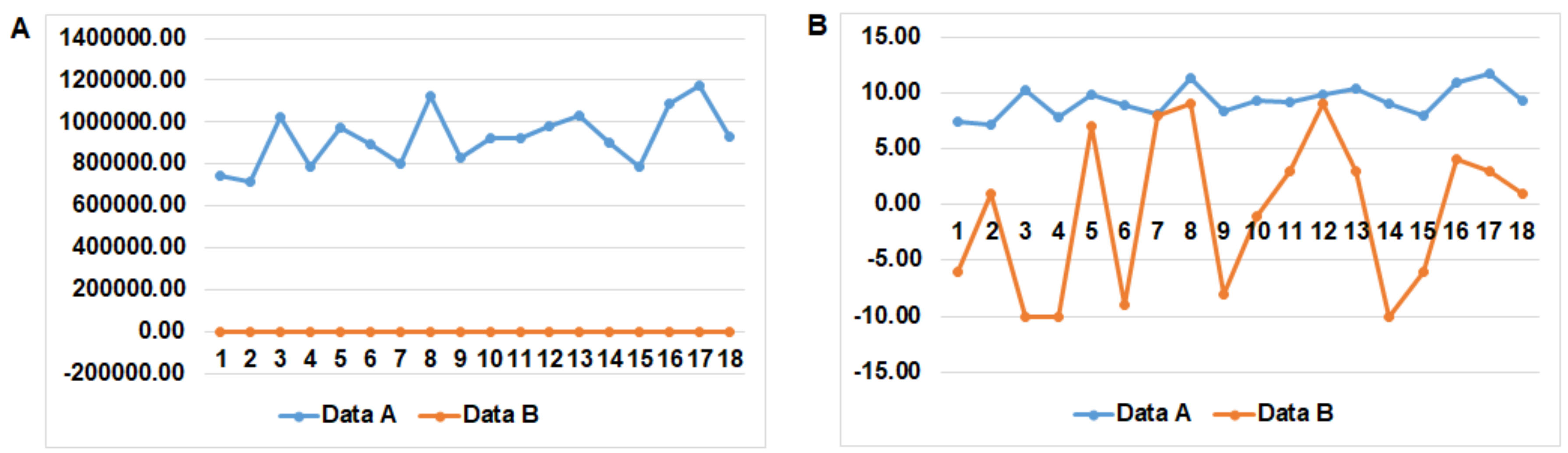
One of the reasons for the use of pre-processing is the need to make data values easier to use by the ANN in the training process. For example, one can think about graphic representation where it would be difficult to represent at the same time two datasets, one with values within [−10; 10] and the other with values within [700,000; 1,200,000]. The first data evolution would be almost impossible to see, read, analyze and process, even though one could use logarithmic representation. For better representation we can simply divide the values of the second dataset by 100,000, thus the new interval that the values belong to would be [7; 12]. Now, it would be much easier to read and examine the evolutions of the two datasets. This example can be considered similar to the need for pre-processing with ANN, as shown in Figure 1.

The Alyuda NeuroIntelligence software offers few algorithms of pre-processing of categorical columns that can be automatically encoded during data pre-processing usage (Alyuda NeuroIntelligence User Manual, 2002, p. 36) [29]:

• One-of-N encoding: Method of encoding categorical columns into numeric ones. Each new numeric column will represent one category from the categorical column data. For example, categorical column Capacity that has High, Medium and Low as its values will be encoded into 3 numeric columns and value High will be represented as {1, 0, 0}, Medium as {0, 1, 0} and Low as {0, 0, 1}.
• Binary encoding means that a column with N distinct categories (values) is encoded into a set of M binary columns, where M is equal to the length of a binary number needed to represent N distinct values. For example, the Color column with values “Red”, “Yellow”, “Green”, “Blue” and “White” will be encoded into 3 binary columns and Red will be represented as {0,0,0}, Yellow as {0,0,1}, Green as {0,1,0}, Blue as {0,1,1}, and White as {1,0,0}.
• Numeric encoding means that a column with N distinct categories (values) is encoded into one numeric column, with one integer value assigned for each category. For example, for the Capacity column with values “Low”, “Medium” and “High”, “Low” will be represented as {1}, Medium as {2}, and High as {3}.

The formula for scaling was provided by Basheer (2001, p. 19) [30]:

$$y_i=z_a+(z_b-z_a)(x_i-x_{max})/(x_{max}-x_{min})$$

(1)

where $y_i$ is the normalized value of $x_i$; $x_{max}$ and $x_{min}$ are the maximum and minimum values of $x_i$; and $z_b$ and $z_a$ are the in interval [$z_b$; $z_a$] corresponding to the range of the transfer function, in our case [−1; 1].

2.3. ANN Design and Structure

ANN has the structure of an organization of neurons in the form of layers. Initial and final layers correspond, respectively, to input data and output data, while the layers between them are hidden layers. The hidden layers are network elements that act as a black box, in the sense that their structure is organized by ANN without being revealed to the user until the end, after its completion and without being altered by the user during processing.

Network interconnections are created so that each neuron in each layer is linked to each neuron in the adjacent layer. Each connection is associated with a weight that is adjusted during the training phase.

Numerous experiences have shown that this type of two-layer ANN has the ability to approximate any nonlinear continuous functions with a certain degree of accuracy determined by a sufficient number of neurons in the hidden layer. The problem in determining network parameters (weights) is a nonlinear optimization task.

The number of hidden artificial neurons determines how ANN works. An increased number of hidden neurons implies an increased potential for determining a solution that is very close to training sets. However, too many hidden neurons can lead, even if within the training set, to a dramatic deviation from the trend of the set in intermediate points or an overly drastic interpretation of the data training. In addition, too many artificial neurons can slow down the processing of training or usage.

A small number of neurons cannot produce the expected necessary correct answers solutions to the problem. It is customary to try multiple configurations to determine the best one. The effectiveness of different configurations can be automatically evaluated by training systems. There are no generally applicable rules for determining these configurations. There are computational algorithms to make it easier to get the number of hidden artificial neurons from configurations structure.

Examples of hidden artificial neurons calculation are:

• Rogers formula: The number of neurons in the hidden layer is obtained by equations involving the number of neurons within the network Borrego (2004, p. 552) [31]:

  $$h=(p-1)m/(n+m+1)$$

  (2)

  where h is the number of neurons in the hidden layer, p is number of training pairs, n is the number of input variables, and m is number of output variables. If the calculation is fulfilled, then the network is correctly determined.
• Hecht–Kolmogorov theory, Hecht (1987, p. 12) [32]:

  $$N_{i+1}=2N_i+1$$

  (3)

  where $N_{i+1}$ is the number of hidden neurons, and $N_i$ is the number of neurons in the previous layer.
• Radial Gaussian system improved by Flood, where the neurons are added in a sequential way, and each neuron is trained starting with the error of its predecessors. The criterion that will stop adding new neurons is the level of accuracy reached by the neurons during the current training session.
• The software dedicated to ANN can also calculate the number of hidden neurons. For example, Alyuda NeuroIntelligence uses two search methods: Heuristic Search makes heuristic search inside a specified search range, which works only for three-layer (one hidden layer) networks; and Exhaustive Search makes exhaustive search among all topologies of the search range you specified, which works for up to five hidden layer networks.

In this case, to improve the results of two above-mentioned search methods:

• We changed fitness criterion.
• We increased search range.
• We reduced search step or accuracy.
• We increased number of retrains per configuration.
• We increased number of iterations per configuration.
• We changed other network training parameters.

The authors, based on their experience working with ANN and Alyuda NeuroInteligence, established a Heuristic Search as the best structure with search accuracy of one unit. The evaluation for the best architecture was a fitness criterion based on training error (the smaller was the error on the training set, the better was the network). After several automatic ANN design calculations, the results of the architecture search (e.g., 4-17-1 structure) were not in line with the initial desire to get a small training error. Therefore, the authors, based on previous research experiences, increased the number of hidden layers from 1 to 2 and reached the final figure of ANN: 4-9-6-1. This change led to an increase in the number of weights from 103 (for the 4-17-1 architecture) to 112. This increase led to a higher structural stability of the initial training and thus a training error within the limits previously imposed. The automatic design search took an average of 4 s for each search and 66 architectures were checked, thus the approximate duration was 4.4 min. However, the time taken to verify the structures sought also must be considered. An average for their time was 20 s for each training and 3 s for each test and validation process (automatic, performed by the software), thus a total of 25.3 min. The time passed for training process was 18 s for all 30,878 iterations (at a speed of 1642.45 iteration/s). For the ANN optimization, the authors used Architecture Search method in the Alyuda NeuroIntelligence software.

Considering the type of data, the objective established and the authors’ experience, the feedforward ANN was chosen for the present research. The detailed information about the ANN’s structure are presented in

Table 2. ANN detailed information. $Source$: Authors’ data representation using Alyuda and Microsoft Office.

ANN Type:	Feedforward	Typology:	Multilayer
Number of input layers:	1	Number of input neurons:	4
Number hidden layers:	2	Number hidden neurons:	15 (9 + 6)
Number of output layers:	1	Number of output neurons:	1
Number of weights:	36-54-6	Number of biases:	9-6-1
Total elements of links between neurons:	36 + 54 + 6 + 9 + 6 + 1 = 112
Hidden layers activation function:	Hyperbolic tangent	Output Activation function:	Logistic
Error function:	Sum-of-squares

.

The values and/or features of ANN’s parameters were selected based only on authors’ research experiences. The feedforward ANN performs nonlinear transformation of input data to approximate data output. The number of input and output neurons is determined by the nature of the problem to be modeled, the type of input data and the form required for network outputs. The number of hidden layers is determined by considering the complexity of the model system and/or the type of problem that must be solved.

2.4. Training

The backpropagation algorithm, which is a descendant gradient technique, is the most popular algorithm training for the feedforward ANN.

Although it was developed by Werbos in 1971 and was rediscovered by Parker in 1982 (Cihocki and Unbehanen, 1993, p. 54) [33], its widespread use is due to Rumellant and his team, who popularized it in the scientific community. Originally made for the feedforward type multi-layer ANN, the algorithm was adapted for ANN feedback type. Backpropagation algorithm can be considered a problem of unconditional optimization for convenient error functions (cost features for example).

Implementing this algorithm requires the exact setting of the activation function and its derivatives. Synaptic weights are usually incrementally modified and the neuron converges to a set of weights that resolve the specific problem. The training samples are cyclically run until the synaptic weights are stabilized, the error for the whole set is acceptably small and the network converges.

Based on the previous experience and the facilities offered by the Alyuda software, the authors preferred the Quick propagation algorithm for the training of the feedforward ANN. Quick propagation algorithm is a heuristic change of Scott Fahlman’s [34] backpropagation algorithm. This training algorithm treats weights as quasi-independent and attempts to use a quadratic simple model to approximate the error area. Even thoguh the algorithm does not have a theoretical foundation, it has proven to be much quicker than the standard backpropagation algorithm for numerous types of problems. However, sometimes the quick propagation algorithm may be unsteady and inclined to lock into local minima.

For the training process, the authors established the following options (cf.

Table 3. Training information. $Source$: Authors’ data representation using Alyuda and Microsoft Office.

Training Algorithm:	Quick Propagation	Modified Method of Weights:	Randomization between ±0.3
Target error value:	0.1	Number of retrains:	1
Learning rate:	0.1	Quick propagation coefficient:	0.75

):

• The maximum error achieved in training process—as absolute error: 0.1.
• Quick propagation coefficient: 0.75. The quick propagation coefficient is a supplementary training parameter. This parameter is used to control (in some situations) the amount of weight growth.
• Learning rate: 0.1 (established for the training process). This is a control parameter that affects the weight change. Higher learning rates result in higher weight changes during each iteration.

The small value of the quick propagation coefficient and the Learning rate were considered due to the need to avoid blocking into local minima and to achieve a smooth training process for better future use of the trained ANN.

2.5. Input Importance

In the training process, the ANN determines the contribution of the input column to the neural network performance. This parameter is called input importance and is calculated using sensitivity analysis techniques. The input importance is shown in Figure 2 and detailed in

Table 4. Input importance. $Source$: Authors’ data representation using Alyuda and Microsoft Office.

Input Column Name	Importance, %
sts_inpr_a	14.60583
rd_e_gerdtot	18.848676
sts_trtu_a	14.005347
lfsi_emp_a	52.540147

.

This input importance will be used in another research and will be a subject for another paper, being analyzed to determine a hierarchy of indicators based on their influence over the economic sentiment indicator. In their future research, the authors will verify this hierarchy developed by the ANN and other hypotheses will be suggested to explain the hierarchy.

2.6. Testing and Validating

The results of training are analyzed with the help of the testing and validation phase. Testing and validation is a process of approximating the quality of the trained neural network. Throughout this process, some data are not fed to the ANN during training process. This set of data is presented to the trained network case by case. Then, the estimating error is measured on each case and used as the approximation of network quality.

2.7. Query

Query presents the possibility of loading new data in the already trained ANN. The loaded data can be the records from the input dataset, thus already fed into the ANN and used for the ANN training, or new data never fed to the ANN, trained or not. The new data must have the same column structure as the training set, being similar to the training dataset, but without the target column or cell for the output data. This must be filled by the simulation of the trained ANN as the result of training.

This process was used by the authors to forecast the value of economic sentiment indicator for 2004, using data for the four other indicators from 2003. The reason for the forecast of 2004 data (and not 2017, for example) or a more appropriate year was that the authors decided to add another difficulty action for the ANN training. Instead of feeding the data to ANN in its initial yearly sequence (from 1999 to 2016), the data were fed in random sequence, not giving to ANN the possibility to learn the trends from the real time sequence, making it more difficult for ANN to understand the influences. Thus, the data never fed to ANN covered 2003 for input data and 2004 for output data. This was one of the objectives of the research.

The value from the 2004 real data for economic sentiment indicator was 95.99, while the simulated data by the ANN was 97.93. Thus, the absolute difference was −1.94 and the relative difference was 2.02%. Bearing in mind that the initial objective was a relative error smaller than 5%, and also considering the testing process with errors smaller than 0.1%, the authors can strongly say that the result of the forecast was a success.

3. Results

3.1. Data Analysis Results

A simple presentation of data analysis made by ANN is presented below as data analysis results:

• 6 columns and 17 rows were analyzed;
• 5 columns and 17 rows were accepted for neural network training;
• 5 numeric columns were sts_inpr_a, rd_e_gerdtot, sts_trtu_a, lfsi_emp_a, and ei_bssi_m_r2;
• Output column was ei_bssi_m_r2;
• Data partition method was random; and
• Data partition results were 13 records to training set (76.47%), 2 records to validation set (11.76%), and 2 records to testing set (11.76%).

3.2. Pre-Processing Results

For the present research, the data were only numerical and the results of their pre-process were as follows:

• Columns before pre-processing: 5;
• Columns after pre-processing: 5;
• Input columns scaling range: [−1..1];
• Output column(s) scaling range: [0..1]; and
• Numeric columns scaling parameters: sts_inpr_a: 0.114286, rd_e_gerdtot: 0.006612, sts_trtu_a: 0.093023, lfsi_emp_a: 0.000118, and ei_bssi_m_r2: 0.026942.

The extended result of the pre-processing process is shown in

Table 5. Result of pre-processing. $Source$: Authors’ data representation using Alyuda and Microsoft Office.

Features	sts_inpr_a	rd_e_ gerdtot	sts_trtu_a	lfsi_emp_a	ei_bssi_m_r2
Parameter	Value	Value	Value	Value	Value
Format	numerical	numerical	numerical	numerical	numerical
Scaling range	[−1; 1]	[−1; 1]	[−1; 1]	[−1; 1]	[0; 1]
Encoded into	1 column	1 column]	1 column	1 column	1 column
Min.	89.8	372.3	94.8	127756	78,866667
Max.	107.3	674.8	116.3	144645	115.983333
Mean	98.105882	528.476471	103.6	138,057.823529	100.498039
Std. deviation	4.50718	96.18759	5.118134	4538.426654	8.432465
Scaling factor	0.114286	0.006612	0093023	0.000118	0.026924

.

3.3. ANN Design and Structure Results

The result of Alyuda Heuristic search gave the best structure of 4-17-1. That corresponds to the structure of an ANN with three layers and four neurons in the input layer (the number of input indicators), seventeen neurons in the hidden layer and one neuron in the output layer (the neuron for the ei_bssi_m_r2). Using this ANN structure in the next phases (training and testing) produced training errors higher than 9%, which was in contradiction with the initial objectives of maximum of 5%.

The authors decided to add and/or remove neurons from the existing single hidden layer and compare the results acquired from the training and testing. After more than 60 attempts, the desired training error was not achieved, thus the authors decided to enlarge the number of hidden layers. In this case, it was not necessary to change the number of hidden neurons, but the way they were organized. The adding of another layer of neurons changed the training process due to the transfer of information through ANN weights. Considering this choice, the authors found the best structure was 4-9-6-1, with five layers with four neurons in the input layer (the number of input indicators), fifteen neurons in two hidden layers (first with nine neurons, and second with six) and one neuron in the output layer (the neuron for the ei_bssi_m_r2). Again, the best structure was determined by tracking the results of training and testing that had to be in concordance with the objectives of the research. The result of the ANN architecture search report was:

• Architecture selected manually;
• 4-9-6-1 architecture selected for training, as presented in Figure 3;
• Hidden layers activation function: Hyperbolic tangent;
• Output parameters: ei_bssi_m_r2;
• Error function: Sum-of-squares; and
• Activation function: Logistic.

3.4. Training Results

The result of the Network training report is presented below:

• Network architecture: [4-9-6-1];
• Training algorithm: Quick Propagation;
• Number of iterations: 30,878;
• Time required: 18 s;
• Training stop reason: Desired error achieved; and
• The best network was tracked and restored.

The training details are shown in

Table 6. Training details. $Source$: Authors’ data representation using Alyuda and Microsoft Office.

Retrains	Iterations	Train Error	Validation Error	Network Error	Test Error
1	30878	0.099	3.035102	0.000028	9.9675
AIC	Correlation	R-Squared	Stop Reason	Error Improvement	Training Speed [iter/s]
160.72	0.999857	0.9994	Desired error achieved	1.49 × 10${}^{-9}$	1642.45

.

AIC (Akaike Information Criterion) is used to compare different networks with different weights (hidden units). With AIC used as fitness criteria during architecture search, simple models are preferred to complex networks if the increased cost of the additional weights (hidden units) in the complex networks does not decrease the network error. It determines the optimal number of weights in the neural network.

Correlation (r) is a statistical measure of strength of the relationship between the actual values and network outputs. The r coefficient can range from −1 to +1. The closer r is to 1, the stronger is the positive linear relationship, and the closer r is to −1, the stronger is the negative linear relationship. When r is near 0, there is no linear relationship.

R-Squared is a statistical ratio that compares model forecasting accuracy with accuracy of the simplest model that just uses the average of all target values as the forecast for all records. The closer this ratio is to 1, the better the model is. Small positive values near zero indicate a poor model. Negative values indicate models that are worse than the simple mean-based model. Do not confuse R-squared with r-squared, which is only a squared correlation.

3.5. Testing and Validating Results

In Figure 4, the evolution of dataset error for both the training (in blue) and the validation sets (in green), recorded in the training phase, is revealed. Obviously, the smaller the errors are, the better is the training result.

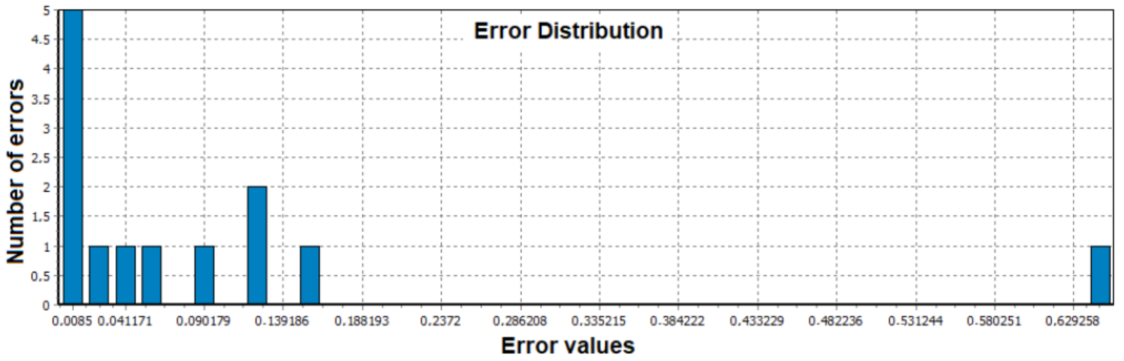
Another representation that shows the evolution of error, in this case the network error, is presented in Figure 5. This figure also can present clues about the suitability of the learning rate option. If the learning rate would have been bigger, the graphic would have been more chaotic with sudden growth and declines that could determine blocking into local minima and the failure of the training.

In Figure 6, the authors display the values distribution of error after 30,878 iterations from the training process (e.g., five data values with absolute error almost 0.0085 and just one data value with absolute error about 0.7).

The errors were calculated as the difference between the real data value and the simulated one during the training process. The results of the testing are presented in

Table 7. Testing results. $Source$: Authors’ data representation using Alyuda and Microsoft Office.

	Target	Output	AE	ARE
Mean:	100.498039	100.238356	1.606193	0.0157
Std Dev:	8.432465	7.297378	3.258939	0.031168
Min:	78.866667	79.520428	0.000332	0.000004
Max:	115.983333	110.293716	10.918265	0.097182
R-squared:	0.752111
Correlation:	0.903756

.

AE is an error value that specifies the “quality” of a neural network training, considered by subtracting the current output values with the target output values of the neural network. The lower the network error is, the better the network had been trained.

ARE (Absolute Relative Error) is an error value that specifies the “quality” of the neural network training. This indicator is calculated by dividing the difference between real and simulated output values by the module of the chosen output value.

In Figure 7, the comparison between real and simulated output values is indicated, after the training process.

Figure 7 displays a line graph of the real and network simulated output values, where the horizontal axis displays the row number of the input dataset and the vertical axis displays the range of the output values. One can choose the representation of one of four input columns against the network simulated output values.

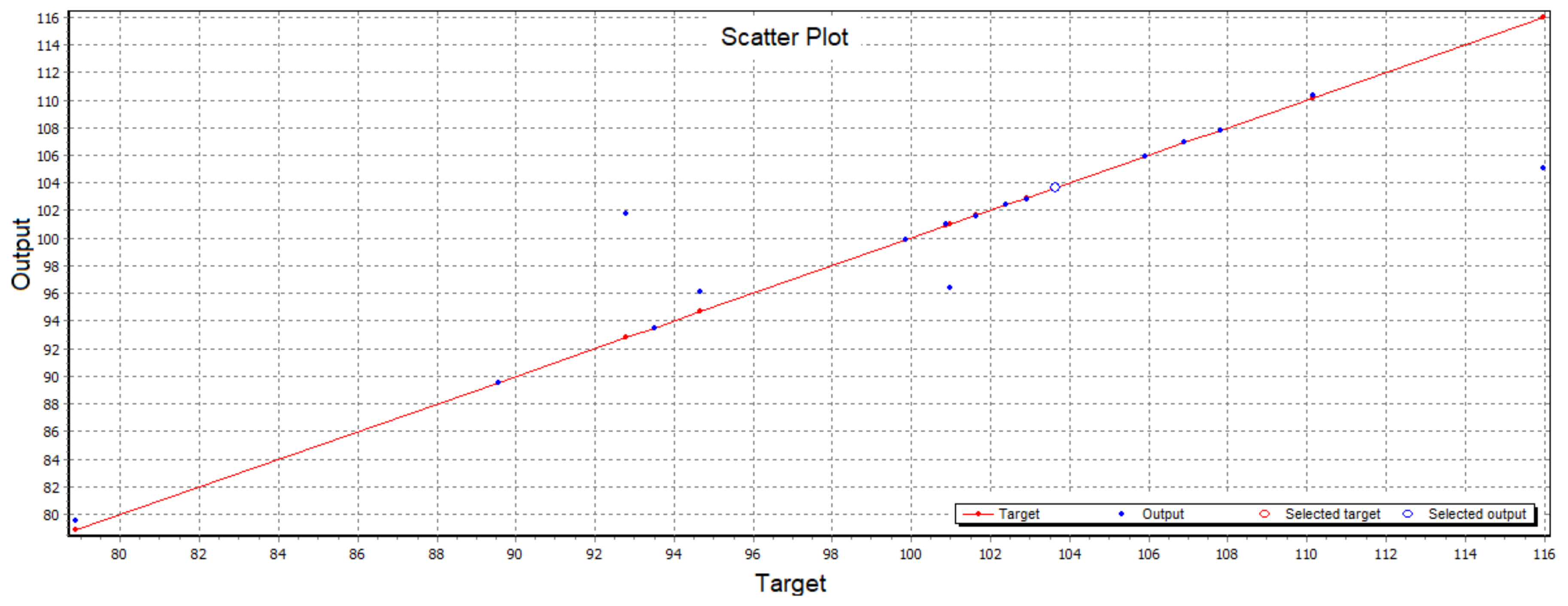
Figure 8 indicates a scatter plot of the actual and forecasted target values, where the horizontal axis displays the actual values and the vertical axis displays the forecasted values. The result of this forecast is presented in

Table 8. Forecast result using a new set of data. $Source$: Authors’ data representation using Alyuda and Microsoft Office.

sts_inpr_a	rd_e_ gerdtot	sts_trtu_a	lfsi_emp_a	ei_bssi_m_r2_ real	ei_bssi_m_r2_ sim
95.7	435.3	102.2	134839.00	95.99	97.93
Absolute Difference:	−1.94
Δ Difference, %:	2.02

.

4. Discussion

Taking into account all of the above results and analyzing all the objectives defined in the beginning of the paper, we can say that all the objectives were achieved. The results of the training, test and query were more than satisfactory.

Considering the results of the present research as well as the previous research on the subject of forecasting the economic sentiment, for future research, we propose that ANN be implemented for the forecast of the indicator for all the EU member countries of the entire euro area. Studies should also be prolonged over a longer period and also on a larger database, including a larger number of influential indicators. This can create a better artificial neural network and therefore a more precise and more important result for training and prognosis.

Finally, a dynamic artificial neural network can be created to train automatically and to determine continuous predictions based on the evolution of the selected influence indicators.

5. Conclusions

The main goal of the research was achieved with high accuracy throughout the training of artificial neural network, which could forecast the value of 2004 sentiment indicator considering the values of the four indicators: volume index of production, intramural R&D expenditure, index of deflated turnover and employment from the year 2003. To validate the results, the following targets were imposed: the result of the neural network training error must be less than 5% and the prediction verification error less than 10%. Considering the transformative power of AI crosses all economic and social sectors, its use as a modern technique for the simulation and/or forecasting of various indicators must be viewed as a tool for sustainable development.

The results of the research presented in this paper are as follows:

• Seventeen records were used (13 records in the training set (76.47%), two records in the validation set (11.76%) and two records in the test set (11.76%)). The data were from Eurostat and include: volume index of production, intramural R&D expenditure, index of deflated turnover and employment and activity influence over the evolution of economic sentiment indicator, from 1999 to 2016.
• Forecasts of the evolution of economic sentiment under the influence of economic indicators of the previous year were sought.
• An artificial neural network was built with the following specifications: 4-9-6-1, i.e., five layers with four neurons in the input layer (the number of input indicators), fifteen neurons in two hidden layers (first layer with nine neurons, and the second layer with six) and one neuron in the output layer (the neuron for the economic sentiment indicator).
• ANN was a feedforward, and the training algorithm was Fahlman’s rapid propagation (backpropagation), with the modification of activation functions such as the hyperbolic tangential function for hiding hidden layers and the logistic function for the exit layer.
• The outcome of the training was more than satisfactory with regard to the defined purpose of the research: training error = 0.099; validation error = 3.035102; and testing error = 9.9675.
• In addition, a quiz test was conducted on the forecast of the economic sentiment indicator for 2004, taking into account the other four indicators in 2003. The test showed an absolute difference of −1.94 and a relative difference of 2.02%.

Some of the advantages of the proposed solution are:

• The ability to predict the results of the influences of the different indices on human decisions, based on artificial intelligence, which copies the biological one and thus is more accurate than decisions made by abstract mathematical methods
• Short simulation, testing and validation time
• The characteristics of the method
• The applicability for different domains

The disadvantages of the proposed solution are:

• ANN’s black box characterization
• Sometimes ANN modeling may take longer
• Need of a minimum number of training-based datasets

For this work, the authors proposed to try to demonstrate the possibility to train and use an ANN to predict the European ESI. Considered as a study to lay the foundations for more in-depth research, the results of this study do not take into account deeper influences among the data used, the values of the training errors, the error of the test/validation, or the artificial neural network type. The authors also did not find similar research in which to predict ESI predictions with the help of ANN, thus they did not compare their method with methods proposed by other researchers.