Comparison of Carbon Emission Reduction Modes: Impacts of Capital Constraint and Risk Aversion

Abstract

The need for low-carbon development has become a social consensus. Increasing numbers of enterprises implement carbon emission reduction by using carbon cap-and-trade mechanisms to cater to consumers and practice social responsibility. From the manufacturer’s perspective, they can implement carbon emission reduction investment by themselves or outsource it to the retailer or energy service company (referred as ESCO). To explore the best carbon emission reduction mode selection strategy, we built and compared three carbon emission reduction modes—manufacturer emission reduction, retailer emission reduction, and ESCO emission reduction—by using Stackelberg game models. The joint decisions of operation, finance, and environment were obtained by using the backward induction approach. The impacts of key parameters were analyzed, such as the retailer’s initial capital amount and the decision-makers’ risk aversion degree on the low carbon supply chain operation. Our results show that the optimal carbon emission reduction mode for the manufacturer is changed as the retailer’s initial capital amount changes. Carbon emission reduction by the ESCO (retailer) becomes the dominant strategy for both the economy and environment when the cost advantage (cash investment ratio) of the ESCO (retailer) carbon emission reduction mode is sufficiently high (low). Overall, decision-makers’ risk aversion is detrimental to both the economic and environmental developments of the supply chain. We also designed contracts to realize the coordination of risk-neutral, risk-averse, capital-adequate, and capital-constrained low-carbon supply chains. These results give guidance for decision-makers to better manage the low-carbon supply chain in the context of fully considering the influential factors of risk aversion and capital constraint.

1. Introduction

Responding to the challenge of environmental pollution and global warming, most countries and economists regard carbon emission reduction as an important strategy. For instance, the European Union’s goal is to reduce carbon emissions by 40% in 2030 compared to the levels from 1990. China has set a target of reducing carbon emissions by 18% in 2020 compared to the levels from 2015. Cap-and-trade regulations have been proven to be an effective mechanism to achieve carbon emission reduction goals [1]. The surplus and lack quotas can be sold and bought by firms on the carbon trading market, respectively.

Another reason to promote implementation of carbon emission reduction for enterprises is the increasing trend in consumers’ environmental awareness and the competitive business environment. Research has shown that 83% of Europeans are attuned to environmental effects, especially carbon footprints, when buying products [2]. More than 27% of consumers in Organization for Economic Cooperation and Development (OECD) countries can be recognized as “green consumers” [3]. To address this trend, most mainstream companies, such as IBM and Wal-Mart, have implemented carbon emission reductions, using the “low-carbon” label for production and sales processes [4].

In general, carbon emission reduction is implemented by carbon-emitting enterprises [5]. In addition, the upstream and downstream enterprises also cooperate to implement carbon emission reduction in joint response to the competitive business environment [6,7]. Third-party energy service companies (ESCOs) are also expected to play an important role in promoting carbon emission reduction efficiency. Research results have estimated that the remaining investment potential in the United States ESCO industry ranges from $71 to $133 billion [8]. The average annual growth rate in the number of ESCOs in China from 2005 to 2013 was 45.42% [9]. Researchers have carried out many studies to make the low-carbon supply chain operation management more efficient and scientific [1,2,3,4,5,6,7,8,9,10,11,12,13,14,15,16,17,18,19,20,21,22,23]. Most of them paid attention to the manufacturer carbon emission reduction mode, but few analyzed retailer and ESCO carbon emission reduction modes. None of them compared these three emission modes. In addition, most of the studies on low-carbon supply chains have assumed that operation enterprises are capital adequate [1,2,3,4,5,6,7,8,9,10,11,12,13,14,15,16,17,18,19,20,21]. These studies ignore the impacts of capital constraint and risk aversion on low-carbon supply chain operation. These are important research gaps in the literature.

The present situation that we cannot neglect is that most of these enterprises are small- and medium-sized enterprises (referred as SMEs). Considering China as an example, the proportion of SMEs is as high as 90%. Most of these enterprises face capital constraint challenges in operations. Trade credit financing has become a common way of managing this challenge [24]. According to the statistics of the National Bureau of Statistics of China, as of 2017, the amount of accounts receivable industrial enterprises above the designated size in China is as high as US $2.15 trillion. For China, this figure corresponds to 16% of gross domestic product (GDP) in 2017. In addition, unpredictable disasters, such as fire, economic crisis, and trade war, have disrupted supply chain operations and brought great losses to enterprises, demonstrating that enterprises need to be more risk averse in their operations [25]. Hence, the assumption of risk neutrality appears to be inadequate for contemporary supply chain management. Empirical findings have provided support for the importance of considering risk preferences in business practices. A research report conducted by McKinsey pointed out that decision makers demonstrate extreme levels of risk aversion regardless of the size of investment by surveying 1500 executives from 90 countries [26]. All participants (the buyer and the seller) must bear some investment risk due to the demand uncertainty in the sales market and the SMEs’ default risk on trade credit transaction forms. The impact of their risk attitudes must be examined. Researchers did lots of research to help managers deal with the impacts of enterprise budget constraints [22,23,24,27,28,29,30,31,32,33,34,35,36,37,38,39,40,41] and risk aversion [25,26,42,43,44,45,46,47,48,49,50,51,52,53] to improve the supply chain operational efficiency. Nevertheless, most of them did not carry out research in combination with a carbon emission reduction strategy.

In this study, we aim to build an operational decision model consisting of one manufacturer, one retailer and one ESCO. The retailer is capital constrained, and the transaction is developed using a trade credit form. Carbon emission reductions can be implemented by the manufacturer (M mode), the retailer (R mode), or the ESCO (E mode). We explore the following research questions.

(1)

How should enterprises make joint decisions about operation, finance, and the environment against the trade credit transaction background? What are the impacts of retailer capital constraints and decision makers’ risk attitudes on low-carbon supply chain operation management?

(2)

Which kind of carbon emission reduction mode (M mode, R mode, or T mode) should be adopted by manufacturers to realize carbon emission reduction?

(3)

How can the trade credit low-carbon supply chain be coordinated?

This research study is expected to guide the development and operation of the interface field of sustainable supply chains and supply chain finance. The remainder of the research study is organized as follows. Section 2 reviews the related literature. Section 3 discusses the assumptions and notations and builds the model. Section 4 analyzes the equilibrium decisions and compares the different carbon emission reduction modes. Section 5 explores the supply chain coordination contract design. Section 6 provides numerical examples examining the propositions. Finally, Section 7 concludes the study and outlines directions for future research. All evidence is provided in the Appendix A.

2. Literature Review

In the next section, we review the literature from three perspectives: carbon emission reduction; integrated management of operation and finance; and the impact of risk attitudes.

2.1. Carbon Emission Reduction

Carbon emission reduction can dramatically impact business operations. Some researchers have addressed this problem from the operation management perspective. From the viewpoint of pricing, inventory, and production decisions, Xu et al. [10] and Xu et al. [11] explored the joint production and pricing problems of the supply chain with cap-and-trade regulation. Hua et al. [12] and Benjaafar et al. [13] investigated the impacts of carbon footprints and strict emission caps on inventory management under carbon-trading regulations, respectively. Research shows that consumer perception is also an important factor affecting the development of enterprise low carbon operation [14,15,16]. Scholars have also extended the research on supply chain structures. Wang et al. [17], He et al. [18], and Yang et al. [19] focused on the reduction in carbon emissions driven by cap-and-trade mechanisms in the dual-channel supply chain, O2O retail supply chain, competing supply chains, and make-to-order supply chain, respectively.

As we can see, most of the literature has assumed that carbon emissions are adopted by carbon-emitting enterprises. Supply chain cooperative emission reduction and ESCO emission reduction are also mainstream emission reduction methods in practice. Zhou et al. [20] analyzed the impacts of cost sharing and co-op advertising on the optimal decisions and coordination of the low-carbon supply chain. Ji et al. [5] found that joint emission reduction by the manufacturer and the retailer is more profitable than the independent emission reduction strategy for all of the supply chain members. Zu et al. [7] found that a cost-sharing contract can motivate the supplier to exert greater emission reduction efforts. Stuart et al. [8], Roshchanka et al. [21], Nolden et al. [2], and Deng et al. [9] analyzed the development status and trends of the United States, Russia, the United Kingdom, and China, respectively.

Conclusively, for the above studies, three shortcomings exist. First, almost all of the above research assumed that enterprises are capital adequate. Second, the studies failed to consider the impact of enterprise risk aversion on carbon emission reduction decisions. Third, the three kinds of carbon emission reduction modes have not been compared in the current research.

2.2. Integrated Management of Operation and Finance

Considering the importance of capital flow to operational decisions, scholars have conducted many research studies on the integrated field of operations and finance. Buzacott et al. [27] explored the inventory decision-making problem under asset financing. Chao et al. [28] and Protopappa-Sieke et al. [29] analyzed the impacts of firms’ capital constraints on the stochastic inventory control problem. Yang et al. [30] found three effects, namely retailer bankruptcy predation, bailouts, and abetment effects. Feng et al. [31] and Yan et al. [32] analyzed the newsboy ordering problem under capital-constraint and information update conditions. Wang et al. [22] found that the capital constraints of manufacturers can encourage them to produce much higher quality re-manufactured products. Sarkar et al. [33] designed a mathematical and analytical approach to better manage the defective items in a multi-stage production system along with budget constraint. In summary, the capital constraints of enterprises have a profound impact on the traditional operation decision making.

Further, scholars have extended the research to the supply chain level. Considering trade credit transaction form, Gupta et al. [24] analyzed the impacts of trade credit periods on the optimal inventory decisions of the supply chain. Luo et al. [34] further extended the research of trade credit finance to the information asymmetry situation. They found that information asymmetry makes the supply chain uncoordinated. Research by Chen et al. [35] found that trade credit finance plays an active role in supply chain coordination. In addition, scholars have designed new contracts to achieve coordination of the trade credit supply chain. For example, Zhang et al. [36] designed a quantity discount contract to coordinate the trade credit supply chain. Wu et al. [37] extended the research to the one supplier, two retailers structure mode and analyzed the impact of retail market competition on trade credit financing. In addition, financing mode comparison is another hot topic of concern to researchers. Current research compared trade credit finance and bank finance. For example, Jing et al. [38], Cai et al. [39], and Kouvelis et al. [40] found that firms’ financing mode selection decisions are determined by factors such as production costs, the capital market competition degree, and enterprise credit ratings, respectively. However, the above research did not consider the impact of capital constraint in green operations of the supply chain. The research that is most related to our study is that of Cao et al. [23]. They analyzed the optimal operation decision and coordination strategy of the emission-dependent supply chain. The authors designed quantity discount contracts, revenue sharing contracts, and buyback contracts to coordinate this kind of supply chain. However, they did not consider the consumer’s perception of the green operation. Nevertheless, the joint decisions and coordination of orders and carbon emission reduction efforts will be more complicated than for single-variable situations; thus, a research gap remains. Previous research has also not considered the impacts of risk aversion on the operations and coordination of low-carbon supply chains. Moreover, the different emission modes have not been compared.

2.3. The Impact of Risk Attitude

Rabe et al. [42] proposed that it was necessary to set the criteria and objectives of measurement before making decisions in the energy sector to avoid risk. The most widely used risk measure criteria in the operational management field are mean-variance (MV), value at risk (VaR), and conditional value at risk (CVaR). In particular, CVaR has advantages in its ability to reflect excess losses, applicability to non-normal distributions, and equivalence to convex programming, which has been widely applied to model risk aversion in economics, finance, and insurance [43]. Gotoh et al. [44] and Chen et al. [45] applied CVaR earlier in the operation management field and used it to describe the impact of newsvendors’ risk aversion on optimal inventory decision making. In follow-up studies, scholars have considered the impact of supply uncertainty [46], sales market competition [47], partial demand information [48], and financial hedging strategy [49] on risk-averse buyers’ optimal decisions. Supply chain coordination and sales discount strategies in risk-averse settings were analyzed by Yang et al. [50] and Ozgun et al. [51]. Furthermore, researchers have made innovations, mainly in the supply chain structure, such as the three-tier [25] and dual-channel supply chains [52]. In addition, Chen et al. [53] designed contracts to realize coordination of the supply chain with risk-aversion manufacturers and risk-aversion retailers. Nevertheless, although existing research has included the impact of decision makers’ risk preferences on operational decisions with the CVaR criterion, few have considered the impacts of a firm’s risk attitude on the operation of green supply chains.

As shown in

Table 1. Comparison between contributions of different literature.

Literature	Carbon Emission Reduction	Integrated Management of Operation and Finance	Risk Attitude	Comparison of Different Carbon Emission Reduction Modes
[1,2,3,4,5,6,7,8,9,10,11,12,13,14,15,16,17,18,19,20,21]	√	×	×	×
[24,27,28,29,30,31,32,33,34,35,36,37,38,39,40,41]	×	√	×	×
[25,26,42,43,44,45,46,47,48,49,50,51,52,53]	×	×	√	×
[22,23]	√	√	×	×
This paper	√	√	√	√

Note: √ and × indicate that the contribution is “Available” or “Not Available” for that research, respectively.

, authors have performed abundant research on the topics of carbon emission reduction [1,2,3,4,5,6,7,8,9,10,11,12,13,14,15,16,17,18,19,20,21], integrated management of operation and finance [24,27,28,29,30,31,32,33,34,35,36,37,38,39,40,41], and risk attitude [25,26,42,43,44,45,46,47,48,49,50,51,52,53], respectively. Nevertheless, few researchers have explored the impacts of capital constraint and risk aversion on the enterprise carbon emission reduction operation. None of them have compared the three different carbon emission reduction modes. The research articles closest to our study are Wang et al. [22] and Cao et al. [23]. They paid attention to the impact of capital constraint on the decision and coordination of the low-carbon supply chain. However, they failed to consider the impact of risk attitude on the enterprise carbon emission reduction operation. They also did not compare the different carbon emission reduction modes. Enterprises do not know how to make an optimal carbon emission reduction effort decision or carbon emission mode selection decision when there are risk-averse members and constrained capital in the supply chain. In this research, we provide the form of an optimal carbon emission reduction effort decision and the condition for enterprises to choose the optimal carbon emission reduction mode by using a mathematical modeling theory and Stackelberg game theory. It fills in the blanks of current theoretical research.

In summary, our research addresses the limitations in current studies by investigating the impacts of capital-constraint and risk-aversion on the low carbon supply chain members’ optimal carbon emission reduction decision, optimal supply chain coordination mechanism, and optimal carbon emission reduction mode selection strategies. Our contributions can be concluded as follows: (1) We are one of the first to compare three kinds of carbon emission modes. (2) We explore the impacts of capital constraint and risk aversion on the operation, decision, coordination, and mode selection of the low-carbon supply chain. (3) We design contracts to coordinate the risk-averse and capital-constrained low-carbon supply chain. The contracts that we designed can also coordinate the joint decisions of the order and carbon emission reduction effort.

3. Model Setup

The basic modeling process is similar to the traditional supply chain research, as performed Ji et al. [7], Cao et al. [23] and Jing et al. [38], among others. The manufacturer $M$ manufactures products with production cost $c$ and sells them to retailer $R$ at wholesale price $w$ (decision variable). The retailer’s order quantity is $q$ (decision variable). He or she sells the products to the consumer market with retail price $p$, and the salvage value of unsold products is $s$.

Similar to Ji et al. [5], Xu et al. [10], Xu et al. [11], Du et al. [14], Xia et al. [16], Wang et al. [17], Wang et al. [22], and Cao et al. [23], the cap-and-trade regulation is used to limit carbon emissions. The manufacturer has initial carbon quotas $e_g$ according to its historical emission data, buys carbon quotas from the carbon trading market when its carbon emissions exceed the “cap”, and sells carbon quotas to the trading market if it has a surplus. The carbon trading price is $t$. The carbon emissions per unit product is $e_0$. To reduce carbon emissions, the manufacturer invests a fixed R&D cost $g_M=0.5k_M{e}_{}^2$ [5,10,16,17] and unit cost per product $c_M$ to employ low-carbon technologies (Mode $M$). Among these costs, the R&D cost $g_M$ consists of cash investment and effort investment [41], and the cash investment proportional of $g_M$ is $\beta$. The carbon emission reduction per unit product is $e$. However, the manufacturer can also outsource the carbon emission reduction directly to ESCO $E$ (Mode E) or retailer $R$ (Mode R) [6,7,8]. The investment costs in Modes E and R are $0.5k_E{e}_{}^2+c_{E}eq$ and $0.5k_R{e}_{}^2+c_{R}eq$, respectively. The carbon trading price among the manufacturer, the retailer, and ESCO is $b$. In addition, since the ESCO is more professional than the manufacturer and the retailer in carbon emission reduction R&D, the emission reduction cost in mode E is the lowest. That is, $k_R\ge k_M\ge k_E$ and $t>b>c_R\ge c_M\ge c_E$ are established.

Some consumers are low-carbon consumers; their low-carbon perception degree is $a$. These consumers’ amount is $ae$ [5,10,16,17]. The remaining consumers’ amount $X$ is uncertain, obeying probability distribution with CDF $\mathrm{F}(\mathrm{X})$, PDF $f(X)$, and IFR $H(X)=\frac{f(X)}{\overline{F}(X)}$. The linear demand functions, which are used by Ji et al. [5], Xia et al. [16], and Wang et al. [17], are inherited in this paper. That is, the total amount of market demand $D=ae+X$.

We adopt a similar method to those used in Chen et al. [35], Wu et al. [37], Jing et al. [38], and Kouvelis et al. [40] to characterize the retailer’s financial situation. The retailer owns initial capital $\eta$. The order will cost the retailer $wq$. In Mode R, the carbon emission reduction will further cost the retailer $0.5\beta k_R{e}_{}^2+c_{R}eq$. That is, if $\eta >wq+(0.5\beta k_R{e}_{}^2+c_{R}eq){|}_{\mathrm{Mode}\begin{array}{c}\end{array}R}$, the retailer is capital adequate, and he or she can execute orders using the initial capital $\eta$ (Mode $A$). However, when $\eta <wq+(0.5\beta k_R{e}_{}^2+c_{R}eq){|}_{\mathrm{Mode}\begin{array}{c}\end{array}\mathrm{R}}$, the retailer is budget constrained to realize orders, and trade credit is used to solve the retailer’s financial problem (Mode $T$). At this time, the manufacturer provides credit line $wq-[\eta -(0.5\beta k_R{e}_{}^2+c_{R}eq){|}_{\mathrm{Mode}\begin{array}{c}\end{array}\mathrm{R}}]$ to the retailer to support the retailer in completing orders and sales. Then, the retailer repays the credit loan using his or her sales revenue.

Thus, it is clear to see that the manufacturer must bear the retailer’s default risk. The retailer’s repayment ability depends on the sales status. If the market demand is less than a critical point $\theta$, the retailer will not be able to fully repay the loan. The sales proceeds will be used to pay off part of the debt [35,37,38,40]. We use ${\alpha }_M$ and ${\alpha }_R$ to depict the manufacturer’s and retailer’s risk attitudes, respectively [43,44,45,46,47,48,49,50,51,52,53]. Let superscripts $T$ and $A$ denote the trade credit and capital-adequate situations and superscripts $E$, $M$, and $R$ denote ESCO carbon emission reduction, manufacturer emission reduction, and retailer emission reduction situations, respectively. Thus, there exists six combinatorial cases: Mode TE, Mode TM, Mode TR, Mode AE, Mode AM, and Mode AR. Let $i$ and $j$ denote the different decision makers and different modes, that is, $i=M,R,E$, $j=TE,TM,TR,AE,AM,AR$.

After analysis, the retailer’s loan amount and sales revenue are $w^{TE,TM}{q}^{TE,TM}-\eta$ and $p\min \{q^{TE,TM},D\}+s{(q^{TE,TM}-D)}^{+}$, respectively. That is, the retailer’s default threshold

$${\theta }^{TE,TM}=\frac{(w^{TE,TM}{q}^{TE,TM}-\eta )-s{q}^{TE,TM}-(p-s)a{e}^{TE,TM}}{p-s}.$$

(1)

The retailer’s loan amount and sales revenue are $w^{TR}{q}^{TR}-\eta +\frac{1}{2}\beta k_R{(e^{TR})}_{}^2+c_R{e}^{TR}{q}^{TR}$ and $p\min \{q^{TR},D\}+s{(q^{TR}-D)}^{+}+e^{TR}{q}^{TR}b$, respectively. The retailer’s default threshold

$${\theta }^{TR}=\frac{(w^{TR}{q}^{TR}-\eta )-s{q}^{TR}-e^{TR}{q}^{TR}(b-c_R)+\frac{1}{2}\beta k_R{(e^{TR})}^2-(p-s)a{e}^{TR}}{p-s}.$$

(2)

The Stackelberg game model is used to depict the relationships of different participants—the manufacturer as the leader, the ESCO, and the retailer as the follower. In the next section, we analyze the optimal operation decisions of different modes.

4. Equilibrium Analysis

4.1. Mode TE

In Mode TE, the ECSO invests cost $c_E{e}^{TE}{q}^{TE}+\frac{1}{2}{k}_E{(e^{TE})}^2$ to obtain $e^{TE}{q}^{TE}$ units of carbon emission permits. The manufacturer pays $c{q}^{TE}$ to manufacture $q^{TE}$ unit production. They buy $e^{TE}{q}^{TE}$ units of carbon from ECSO by using $b{e}^{TE}{q}^{TE}$, and buy $(e_0-e^{TE})q^{TE}-e_g$ units of carbon (sells $e_g-(e_0-e^{TE})q^{TE}$ units of carbon) through the carbon trading market with trading price $t$. The manufacturer receives the retailer’s initial capital $\eta$ at the beginning of the transaction. Then, if the stochastic market demand $X$ is below the retailer’s default threshold ${\theta }^{TE}$, the retailer is bankrupt. Their sales revenue $pX+s(q^T-X)-c{q}^{TE}$ is used to repay the manufacturer’s credit loan. If $X$ is higher than ${\theta }^{TE}$, the retailer is able to fulfil their repayment obligations. The manufacturer obtains $w^{TE}{q}^{TE}-\eta$. If $X$ is higher than $<q^{TE}-a{e}^{TE}$, the retailer pays ordering cost $w^{TE}{q}^{TE}$ and obtains sales revenue $p{q}^{TE}$. To summarize the above analysis, the manufacturer, the retailer, and the ESCO’s profits can be depicted by

$${\pi }_M^{TE}=\{\begin{array}{l}\eta +pX+s(q^T-X)-c{q}^{TE}-b{e}^{TE}{q}^{TE}-t((e_0-e^{TE})q^{TE}-e_g),X<{\theta }^{TE},\\ (w^{TE}-c)q^{TE}-b{e}^{TE}{q}^{TE}-t((e_0-e^{TE})q^{TE}-e_g),X\ge {\theta }^{TE},\end{array}$$

(3)

$${\pi }_R^{TE}=\{\begin{array}{l}-\eta ,X<{\theta }^{TE},\\ -\eta +p(a{e}^{TE}+X)+s(q^{TE}-X-a{e}^{TE})-(w^{TE}{q}^{TE}-\eta ),{\theta }^{TE}\le X<q^{TE}-a{e}^{TE},\\ (p-w^{TE}{q}^{TE})q^{TE},X\ge q^{TE}-a{e}^{TE},\end{array}$$

(4)

$${\mathsf{\Pi }}_E^{TE}=(b-c_E)e^{TE}{q}^{TE}-\frac{1}{2}{k}_E{(e^{TE})}^2.$$

(5)

In the decentralized supply chain, the manufacturer decides the optimal wholesale price first. Then, the retailer and ESCO decide the optimal order quantity and carbon emission reduction effort level, respectively. The optimal equilibrium operation decisions can be obtained by applying the backward induction method. Referring to the literature [43,44,45,46,47,48,49,50,51,52,53], we use the CVaR criterion to characterize the decision-makers’ risk attitudes. Let $\tilde{F}(\cdot )={\alpha }_R-F(\cdot )$, ${\tau }_i=1/{\alpha }_i$. The retailer and ESCO’s optimal decisions satisfy the following proposition.

Proposition 1. 

The retailer’s optimal order quantity$q^{TE\ast }$and the ESCO’s global optimal carbon emission reduction effort$e^{TE\ast }$in TE mode under CVaR criterion satisfy

$$(p-s)(1-\frac{a(b-c_E)}{k_E})\tilde{F}((1-\frac{a(b-c_E)}{k_E})q^{TE\ast })=(w^{TE}-s-\frac{a(p-s)(b-c_E)}{k_E})\tilde{F}({\theta }^{TE}(q^{TE\ast }))=0,$$

(6)

$$e^{TE\ast }=(b-c_E)q^{TE\ast }/k_E.$$

(7)

Corollary 1. 

The$q^{TE\ast }$is increasing in$e^{TE\ast }$. The$q^{TE\ast }$and$e^{TE\ast }$are increasing in${\alpha }_R$and decreasing in$\eta$and$w^{TE}$.

Corollary 1 indicates that the retailer’s order quantity is increasing in his or her risk aversion factor and decreasing in his or her initial capital amount because the risk faced by the retailer is the product’s unmarketable risk. The risk-averse retailer will choose to decrease the order quantity to avoid over-order risk. The lower that the retailer’s initial capital is, the more that the retailer will be inclined to use trade credit finance, which is equivalent to the manufacturer sharing more market risk with the retailer. The retailer tends to order more product. At this time, the manufacturer needs more carbon quotas to complete production. To reduce the carbon emission cost, the manufacturer will buy more carbon from the ESCO, which will encourage the ESCO to improve the carbon emission reduction effort.

Similar to Proposition 1, the manufacturer’s utility function in Mode TE under CVaR criteria can be obtained as follows:

$${\mathsf{\Pi }}_M^{TE}=(w^{TE}-c)q^{TE}-{\tau }_M(p-s){\displaystyle {\int }_0^{{\theta }^{TE}}F(x)dx}-b{e}^{TE}{q}^{TE}-t((e_0-e^{TE})q^{TE}-e_g).$$

(8)

The optimal wholesale price decision $w^{TE\ast }$ can be determined further.

Proposition 2. 

When$H(X)$is convex increasing in$X$, there exists threshold${\widehat{t}}_1$, such that when$t<{\widehat{t}}_1$,${\mathsf{\Pi }}_M^{TE}$is concave in$w^{TE}$. The global optimal wholesale price$w^{TE\ast }$satisfies

$$\begin{array}{l}\frac{(p-s)A_2(w^{TE\ast })\overline{F}({\theta }^{TE})(1-A_3{q}^{TE\ast }H(A_3{q}^{TE\ast }(w^{TE\ast })))}{(p-s)-A_2(w^{TE\ast })q^{T\ast }(w^{TE\ast })H({\theta }^{TE}(w^{TE\ast }))}\\ \begin{array}{cccc}& & & \end{array}=((c-s)-\frac{a(p-s)(b-c_E)}{k_E}-\frac{2(t-b)(b-c_E)}{k_E}{q}^{TE\ast }(w^{TE\ast })).\end{array}$$

(9)

4.2. Mode TM

In Mode TM, the manufacturer implements carbon emission reduction by themselves. The manufacturer decides the optimal wholesale price and carbon emission reduction effort decisions first; then, the retailer makes the optimal order decision. Similar to the cost analysis in Section 4.1, the manufacturer and the retailer’s profit functions can be depicted by

$${\pi }_M^{TM}=\{\begin{array}{l}\eta +pX+s(q^{TM}-X)-c{q}^{TM}-c_M{e}^{TM}{q}^{TM}-t((e_0-e^{TM})q^{TM}-e_g)-\frac{1}{2}{k}_M{(e^{TM})}^2,X<{\theta }^{TM},\\ (w^{TM}-c)q^{TM}-c_M{e}^{TM}{q}^{TM}-t((e_0-e^{TM})q^{TM}-e_g)-\frac{1}{2}{k}_M{(e^{TM})}^2,X\ge {\theta }^{TM},\end{array}$$

(10)

$${\pi }_R^{TM}=\{\begin{array}{l}-\eta ,X<{\theta }^{TM},\\ -\eta +p(a{e}^{TM}+X)+s(q^{TM}-X-a{e}^{TM})-(w^{TM}{q}^{TM}-\eta ),{\theta }^{TM}\le X<q^{TM}-a{e}^{TM},\\ -\eta +p{q}^{TM}-(w^{TM}{q}^{TM}-\eta ),X\ge q^{TM}-a{e}^{TM}.\end{array}$$

(11)

Similar to Proposition 1, the manufacturer and retailer’s conditional values at risk can be obtained as follows,

$${\mathsf{\Pi }}_R^{TM}=-\eta +(p-s)(q^{TM}-a{e}^{TM}-{\theta }^{TM})-{\tau }_R(p-s){\displaystyle {\int }_{{\theta }^{TM}}^{q^{TM}-a{e}^{TM}}F(x)dx},$$

(12)

$${\mathsf{\Pi }}_M^{TM}=(w^{TM}-c)q^{TM}-{\tau }_M(p-s){\displaystyle {\int }_0^{{\theta }^{TM}}F(x)dx}-c_M{e}^{TM}{q}^{TM}-t((e_0-e^{TM})q^{TM}-e_g)-\frac{1}{2}{k}_M{(e^{TM})}^2.$$

(13)

After analysis, the optimal decisions in the equilibrium state satisfy the following proposition.

Proposition 3. 

If$H(x)$is increasing convex function in$x$, there exists threshold${\widehat{t}}_2$, such that when$t<{\widehat{t}}_2$, the global optimal order, wholesale price, and carbon emission reduction effort decisions$(q^{TM\ast },w^{TM\ast },e^{TM\ast })$satisfy

$$(p-s)\tilde{F}(q^{TM\ast }-a{e}^{TM\ast })=(w^{TM\ast }-s)\tilde{F}({\theta }^{TM}),$$

(14)

$$\begin{array}{l}((t-c_M)e^{TM\ast }-(w^{TM\ast }-s)F({\theta }^{TM}))((p-s)-q^{TM\ast }H({\theta }^{TM}))+\\ q^{TM\ast }\tilde{F}({\theta }^{TM})(A_2((w^{TM\ast }-s)H({\theta }^{TM})-(p-s)H(A_3{q}^{TM\ast })))=0,\end{array}$$

(15)

$$\begin{array}{l}(t-c_M)e^{TM\ast }(a(p-s)H({\theta }^{TM}))+(a(p-s)F({\theta }^{TM})+\\ (t-c_M)q^{TM\ast }-k_M{e}^{TM\ast })((w^{TM\ast }-s)H({\theta }^{TM})-(p-s)H(A_3{q}^{TM\ast }))=0.\end{array}$$

(16)

Corollary  2. 

The$q^{TM\ast }$increases in$e^{TM}$and${\alpha }_R$, and decreases in$\eta$and$w^{TM}$.

4.3. Mode TR

In Mode TR, carbon emission reduction is implemented by the retailer. In this mode, the manufacturer decides the optimal wholesale price first, and the retailer then makes joint decisions about the order and carbon emission reduction effort. The manufacturer and the retailer’s profit functions can be obtained as follows:

$${\pi }_R^{TR}=\{\begin{array}{l}-\eta -\frac{1}{2}(1-\beta )k_R{(e_{}^{TR})}^2,X<{\theta }^{TR},\\ -\frac{1}{2}{k}_R{(e_{}^{TR})}^2+p(a{e}_{}^{TR}+X)+s(q^{TR}-X-a{e}^{TR})+e_{}^{TR}{q}_{}^{TR}(b-c_R)-w^{TR}{q}^{TR},{\theta }^{TR}\le X<q^{TR}-a{e}^{TR},\\ (p-w^{TR})q^{TR}-e_{}^{TR}{q}_{}^{TR}(b-c_R)-\frac{1}{2}{k}_R{(e_{}^{TR})}^2,X\ge q^{TR}-a{e}^{TR},\end{array}$$

(17)

$${\pi }_M^{TR}=\{\begin{array}{l}\eta -\frac{1}{2}\beta k_R{(e^{TR})}^2+p(a{e}^{TR}+X)+s(q^{TR}-a{e}^{TR}-X)-c{q}^{TR}-b{e}^{TR}{q}^{TR}-t((e_0-e^{TR})q^{TR}-e_g),X<{\theta }^{TR},\\ (w^{TR}-c)q^{TR}-b{e}^{TR}{q}^{TR}-t((e_0-e^{TR})q^{TR}-e_g),X\ge {\theta }^{TR}.\end{array}$$

(18)

Their CVaR utility functions can be determined by

$${\mathsf{\Pi }}_R^{TR}=-\eta +(p-s)(q^{TR}-a{e}^{TR}-{\theta }^{TR})-{\tau }_R(p-s){\displaystyle {\int }_{{\theta }^{TR}}^{q^{TR}-a{e}^{TR}}F(x)dx}-\frac{1}{2}(1-\beta )k_R{(e^{TR})}^2,$$

(19)

$${\mathsf{\Pi }}_M^{TR}=(w^{TR}-c)q^{TR}-{\tau }_M(p-s){\displaystyle {\int }_0^{{\theta }^{TR}}F(x)dx}-b{e}^{TR}{q}^{TR}-t((e_0-e^{TR})q^{TR}-e_g).$$

(20)

Proposition 4. 

(i) There exists threshold${\widehat{b}}_1$, such that when$b<{\widehat{b}}_1$, the retailer’s global optimal order decision and carbon emission reduction decision$q^{TR\ast }$and$e^{TR\ast }$satisfy

$$\{\begin{array}{l}{\tau }_R((q^{TR\ast }(b-c_R)-k_R\beta e^{TR\ast }+(p-s)a)\tilde{F}({\theta }^{TR}(q^{TR\ast },e^{R\ast }))-a(p-s)\tilde{F}(q^{TR\ast }-a{e}^{TR\ast }))-k_R(1-\beta )e^{TR\ast }=0,\\ (p-s)\tilde{F}(q^{TR\ast }-a{e}^{R\ast })-((w^{TR}-s)-e^{TR\ast }(b-c_R))\tilde{F}({\theta }^{TR}(q^{TR\ast },e^{R\ast }))=0.\end{array}$$

(21)

(ii) Threshold${\widehat{t}}_3$exists such that when$t<{\widehat{t}}_3$, the manufacturer’sglobal optimal wholesale price$w^{TR\ast }$satisfies

$$\begin{array}{l}{\tau }_M(p-s)q^{TR\ast }({\alpha }_M-F({\theta }^{TR}))+((p-s)(w^{TR\ast }-c)-{\tau }_M(p-s)F({\theta }^{TR})((w^{TR\ast }-s)-e^{TR\ast }(b-c_R))+\\ (t-b)e^{TR\ast }(p-s))\frac{d{q}^{TR\ast }}{d{w}^{TR}}+((p-s)(t-b)q^{TR\ast }-{\tau }_M(p-s)F({\theta }^{TR})(\beta k_R{e}^{TR\ast }-q^{TR\ast }(b-c_R)))\frac{d{e}^{TR\ast }}{d{w}^{TR}}=0,\end{array}$$

(22)

where$\frac{d{q}^{TR\ast }}{d{w}^{TR}}$and$\frac{d{e}^{TR\ast }}{d{w}^{TR}}$are the solutions to the following equations:

$$\{\begin{array}{l}{\tau }_R((\frac{d{q}^{TR\ast }}{d{w}^{TR}}(b-c_R)-k_R\beta \frac{d{e}^{TR\ast }}{d{w}^{TR}})\tilde{F}({\theta }^{TR})-\frac{(q(b-c_R)-k_R\beta e^{TR\ast }+(p-s)a)f({\theta }^{TR})}{p-s}\frac{d{\theta }^{TR}}{d{w}^{TR}}+\\ a(p-s)(\frac{d{q}^{TR\ast }}{d{w}^{TR}}-a\frac{d{e}^{TR\ast }}{d{w}^{TR}}))-k_R(1-\beta )\frac{d{e}^{TR\ast }}{d{w}^{TR}}=0,\\ ((w^{TR}-s)-e^{TR\ast }(b-c_R))f({\theta }^{TR})\frac{d{\theta }^{TR}}{d{w}^{TR}}-(p-s)f(q^{TR\ast }-a{e}^{TR\ast })(\frac{d{q}^{TR\ast }}{d{w}^{TR}}-a\frac{d{e}^{TR\ast }}{d{w}^{TR}})-\\ (1-(b-c_R)\frac{d{e}^{TR\ast }}{d{w}^{TR}})\tilde{F}({\theta }^{TR})=0,\\ \frac{d{\theta }^{TR}}{d{w}^{TR}}=\frac{q^{TR\ast }+((w^{TR\ast }-s)-e^{TR\ast }(b-c_R))\frac{d{q}^{TR\ast }}{d{w}^{TR}}+(\beta k_R{e}^{TR\ast }-q^{TR\ast }(b-c_R))\frac{d{e}^{TR\ast }}{d{w}^{TR}}}{p-s}.\end{array}$$

Actually, Cao et al. [23], Wu et al. [37], Jing et al. [38], and Kouvelis et al. [40] have given joint optimal decisions of wholesale price and order quantity when the retailer is capital constrained. Through the above analysis, we give the joint optimal decisions of wholesale price, order quantity, and carbon emission reduction effort when the retailer is capital constrained. Our results are more general than those in the previous studies, which are simultaneously applicable to risk-neutral and risk-averse situations. In addition, the optimal decision formed under three different carbon emission modes are given in turn, which is also an innovation compared to the current research. In the next section, we provide a supplementary analysis to the capital-adequate situation.

4.4. Mode A

In Mode A, the manufacturer and retailer’s CVaR utility functions in the EA, MA, and RA modes are

$${\mathsf{\Pi }}_R^{EA}=(p-w^{EA})q^{EA}-{\tau }_R(p-s){\displaystyle {\int }_0^{q^{EA}-a{e}^{EA}}F(x)}dx,$$

(23)

$${\mathsf{\Pi }}_M^{EA}=(w^{EA}-c)q^{EA}-b{e}^{EA}{q}^{EA}-t((e_0-e^{EA})q^{EA}-e_g),$$

(24)

$${\mathsf{\Pi }}_E^{EA}=(b-c_E)e^{EA}{q}^{EA}-\frac{1}{2}{k}_E{(e^{EA})}^2,$$

(25)

$${\mathsf{\Pi }}_R^{MA}=(p-w^{MA})q^{MA}-{\tau }_R(p-s){\displaystyle {\int }_0^{q^{MA}-a{e}^{MA}}F(x)}dx,$$

(26)

$${\mathsf{\Pi }}_M^{MA}=(w^{MA}-c)q^{MA}-c_M{e}^{MA}{q}^{MA}-t((e_0-e^{MA})q^{MA}-e_g)-\frac{1}{2}{k}_M{(e^{MA})}^2,$$

(27)

$${\mathsf{\Pi }}_R^{RA}=(p-w^{RA})q^{RA}-{\tau }_R(p-s){\displaystyle {\int }_0^{q^{RA}-a{e}^{RA}}F(x)}dx+(b-c_R)e^{RA}{q}^{RA}-\frac{1}{2}{k}_R{(e^{RA})}^2,$$

(28)

$${\mathsf{\Pi }}_M^{RA}=(w^{RA}-c)q^{RA}-b{e}^{RA}{q}^{RA}-t((e_0-e^{RA})q^{RA}-e_g).$$

(29)

Let $A_4=1-a(b-c_E)/k_E$. Brief backward induction can be used to determine the equilibrium decisions in Mode A, satisfying Proposition 5.

Proposition 5. 

(i) There exists threshold${\widehat{t}}_4$, such that when$t<{\widehat{t}}_4$, the ESCO, the retailer, and the manufacturer’s global optimal carbon emission reduction effort, order quantity, and wholesale price decisions in Mode AE satisfy

$$q^{AE\ast }=\frac{1}{A_4}{F}^{-1}(\frac{p-w^{AE\ast }}{A_4{\tau }_R(p-s)}),$$

(30)

$$e^{AE\ast }=(b-c_E)q^{AE\ast }/k_E,$$

(31)

$$w^{AE\ast }=c+A_4{\tau }_R(p-s)q^{AE\ast }f(A_4{q}^{AE\ast })+2(b+t)A_4{q}^{AE\ast }-t{e}_0.$$

(32)

(ii) There exists threshold${\widehat{t}}_5$, such that when$t<{\widehat{t}}_5$, the retailer and the manufacturer’s global optimal order quantity and wholesale price and carbon emission reduction effort decisions in Mode AM satisfy

$$(p-w^{AE\ast })-{\tau }_R(p-s)F(q^{AE\ast }-a{e}^{AE\ast })=0,$$

(33)

$$(w^{AE\ast }-c-c_M{e}^{AE\ast }-t(e_0-e^{AE\ast }))-{\tau }_R(p-s)q^{AE\ast }f(q^{AE\ast }-a{e}^{AE\ast })=0,$$

(34)

$$(w^{AE\ast }-c-c_M{e}^{AE\ast }-t(e_0-e^{AE\ast }))a+(t-c_M)q^{AE\ast }-k_E{e}^{AE\ast }=0.$$

(35)

(iii) There exist thresholds${\widehat{b}}_2$,${\widehat{t}}_6$, such that when$b<{\widehat{b}}_2$,$t<{\widehat{t}}_6$, the retailer and the manufacturer’s global optimal order quantity, carbon emission reduction efforts, and wholesale price decisions in Mode AR satisfy

$$(p-w^{AR\ast })-{\tau }_R(p-s)F(q^{AR\ast }-a{e}^{AR\ast })=0,$$

(36)

$$a{\tau }_R(p-s)F(q^{AE\ast }-a{e}^{AE\ast })+(b-c_R)q^{AE\ast }-k_R{e}^{AE\ast }=0,$$

(37)

$$q^{AR\ast }+((w^{AR\ast }-c)-b{e}^{AR\ast }-t(e_0-e^{AR\ast }))\frac{d{q}^{AR\ast }}{d{w}^{AR}}+(t-b)q^{AR\ast }\frac{d{e}^{AR\ast }}{d{w}^{AR}},$$

(38)

where$\frac{d{q}^{AR\ast }}{d{w}^{AR}}$and$\frac{d{e}^{AR\ast }}{d{w}^{AR}}$satisfy

$$\{\begin{array}{l}-1-{\tau }_R(p-s)f(q^{AR\ast }-a{e}^{AR\ast })\frac{d{q}^{AR\ast }}{d{w}^{AR}}+(a{\tau }_R(p-s)f(q^{AR\ast }-a{e}^{AR\ast })+(b-c_R))\frac{d{e}^{AR\ast }}{d{w}^{AR}}=0,\\ (a{\tau }_R(p-s)f(q^{AR\ast }-a{e}^{AR\ast })+(b-c_R))\frac{d{q}^{AR\ast }}{d{w}^{AR}}-(a^2{\tau }_R(p-s)f(q^{AR\ast }-a{e}^{AR\ast })+k)\frac{d{e}^{AR\ast }}{d{w}^{AR}}=0.\end{array}$$

4.5. Centralized Supply Chain

A centralized supply chain can be easily defined as the expected total utility of the supply chain when all of the agents are risk neutral. Nevertheless, this definition might not carry over to cases in which the agents are risk averse. The concept of Pareto optimality defined by Chen et al. [53] is used to describe the objective function of the centralized supply chain with risk averse agents. Under CVaR objectives, Pareto optimality is equivalent to maximizing the sum of the objectives of all agents. Let $k=E,M,R$, we have ${\mathsf{\Pi }}_{}^{Cl}={\mathsf{\Pi }}_M^l+{\mathsf{\Pi }}_R^l+{\mathsf{\Pi }}_E^l{|}_{\mathrm{Mode} \mathrm{E}}$. It is easy to verify that $\frac{d{\mathsf{\Pi }}_{}^{Cl}}{d{\alpha }_i}>0,\frac{d{\mathsf{\Pi }}_{}^{Cl}}{d{\alpha }_i}>0,\frac{d{\mathsf{\Pi }}_{}^{Cl}}{d{\alpha }_i}>0$ are established according to the Envelope theorem.

Define ${\alpha }_C^{}=\max \{{\alpha }_M,{\alpha }_R\}$; the utility function of the centralized supply chain can be defined as

$$\begin{array}{l}{\mathsf{\Pi }}_{}^{Cl}={\mathsf{\Pi }}_M^l+{\mathsf{\Pi }}_R^l+{\mathsf{\Pi }}_E^l\\ =(p-c)q^{Cl}-{\tau }_l(p-s){\displaystyle {\int }_0^{q^{Cl}-a{e}^{Cl}}F(x)dx}-c_l{e}^{Cl}{q}^{Cl}-t((e_0-e^{Cl})q^{Cl}-e_g)-\frac{1}{2}{k}_l{(e^{Cl})}^2.\end{array}$$

(39)

The optimal operational decisions in the centralized supply chain can be determined as follows.

Proposition 6. 

There exists threshold${\widehat{t}}_7$, such that when$t<{\widehat{t}}_7$, the global optimal order decision$q^{Cl\ast }$and carbon emission reduction effort decision$e^{Cl\ast }$satisfy

$$(p-c)-{\tau }_k(p-s)F(q^{Ck\ast }-a{e}^{Ck\ast })-c_k{e}^{Ck\ast }-t(e_0-e^{Ck\ast })=0,$$

(40)

$$e^{Ck\ast }=\frac{k_l-a(t-c_l)}{a((p-c)-t{e}_0)+(t-c_l)q^{Cl\ast }}.$$

(41)

4.6. Sensitivity Analysis

To analyze the impacts of capital constraints and risk attitudes and to compare the different carbon emission reduction modes, we perform sensitivity analysis in the next section. First, we analyze the parameters of the retailer’s initial capital amount.

Proposition 7. 

(i) 

If${\alpha }_M\ge {\alpha }_R$,$\eta \to 0$, then$w^{TM\ast }\to p$,$q^{TM\ast }\to q^{CM\ast }$,$e^{TM\ast }\to e^{CM\ast }$,${\mathsf{\Pi }}_M^{TM\ast }\to {\mathsf{\Pi }}_M^{CM\ast }$,${\mathsf{\Pi }}_R^{TM\ast }\to 0$are established.

(ii) 

If${\alpha }_M\ge {\alpha }_R$,$\eta \to 0$, then$w^{TE\ast }\to p$,$q^{TE\ast }<q^{CE\ast }$,$e^{TE\ast }<e^{CE\ast }$,${\mathsf{\Pi }}_M^{TE\ast }<{\mathsf{\Pi }}_M^{CE\ast }$,${\mathsf{\Pi }}_R^{TE\ast }\to 0$are established.

(iii) 

If${\alpha }_M\ge {\alpha }_R$,$\eta \to 0$,$\beta \to 0$,$c_R\to 0$, then$w^{TR\ast }\to p$,$q^{TR\ast }\to q^{CR\ast }$,$e^{TR\ast }\to e^{CR\ast }$,${\mathsf{\Pi }}_M^{TR\ast }\to {\mathsf{\Pi }}_M^{CR\ast }$,${\mathsf{\Pi }}_R^{TR\ast }\to 0$are established.

(iv) 

If${\alpha }_M<{\alpha }_R$,$\eta \to 0$, then inequalities${\mathsf{\Pi }}_M^{TM\ast }<{\mathsf{\Pi }}_M^{CM\ast },{\mathsf{\Pi }}_M^{TE\ast }<{\mathsf{\Pi }}_M^{CE\ast }$are established.

(v) 

If${\alpha }_M<{\alpha }_R$,$\eta \to 0$,$\beta \to 0$,$c_R\to 0$, then inequality${\mathsf{\Pi }}_M^{TR\ast }<{\mathsf{\Pi }}_M^{CR\ast }$is established.

We analyzed an extreme case in which $\eta \to 0$ in Proposition 7. Wu et al. [37] have proven that the wholesale price is increasing compared to the retail price level when the retailer’s initial capital amount is closing to zero by using numerical analysis method. We found some new insights through deduction. First, the order quantity decision and the carbon emission reduction effort level will increase to a very high level, e.g., the centralized supply chain decision level, when $\eta \to 0$. At this time, the manufacturer’s CVaR utility also similarly increases to the centralized supply chain utility level. In contrast, the retailer’s utility is decreased to 0 because when the retailer’s initial capital amount is low, he or she is more inclined to default on the loan, indicating that the manufacturer shares more market risk with the retailer at this time, encouraging the retailer to order more products. The manufacturer will increase the wholesale price to cover the increase in the retailer’s default risk. When the yield quantity increases, the carbon emissions are increased accordingly. Carbon emission reduction becomes profitable for the manufacturer. Then, the carbon emission reduction effort level also increases. Finally, the increases in the wholesale price, order quantity, and carbon emission reduction level cause the manufacturer’s profit to increase and the retailer’s profit to decrease. The above analysis indicates that no matter which kind of carbon emission mode is used, the carbon emission reduction investor should pay more for carbon emission reduction efforts when the retailer has a low initial capital.

Second, in the risk-averse setting, the trade credit contract cannot realize the coordination of the supply chain. Most of the studies, such as Chen et al. [35] and Zhang et al. [36], have indicated that the supply chain is coordinated by the trade credit contract when $\eta \to 0$. Their research was based on the condition that the participants are risk neutral. In Proposition 7(iv) and (v), we find that the trade credit contract’s coordinative role is invalid when the supplier is more risk averse than the retailer (${\alpha }_M<{\alpha }_R$).

Proposition 8. 

When${\alpha }_M\ge {\alpha }_R$, there exists a threshold$\widehat{\eta }$, such that the following applies:

(i) 

If$\eta <\widehat{\eta }$, then inequalities$e_{}^{TM\ast }>e_{}^{AM\ast }$,$e_{}^{TE\ast }>e_{}^{AE\ast }$,${\mathsf{\Pi }}_M^{TM\ast }>{\mathsf{\Pi }}_M^{AM\ast }$,${\mathsf{\Pi }}_M^{TE\ast }>{\mathsf{\Pi }}_M^{AE\ast }$,${\mathsf{\Pi }}_R^{AM\ast }>{\mathsf{\Pi }}_R^{TM\ast }$,${\mathsf{\Pi }}_R^{AE\ast }>{\mathsf{\Pi }}_R^{TE\ast }$are established.

(ii) 

If$\beta \to 0$,$c_R\to 0$,$\eta <\widehat{\eta }$,then inequalities$e_{}^{TR\ast }>e_{}^{AR\ast }$,${\mathsf{\Pi }}_M^{TR\ast }>{\mathsf{\Pi }}_M^{AR\ast }$,${\mathsf{\Pi }}_R^{AR\ast }>{\mathsf{\Pi }}_R^{TR\ast }$are established.

(iii) 

If$k_M=k_E,c_M=c_E$,$\eta <\widehat{\eta }$,then inequalities$e_{}^{TM\ast }>e_{}^{TE\ast }$,${\mathsf{\Pi }}_M^{TM\ast }>{\mathsf{\Pi }}_M^{TE\ast }$are established.

(iv) 

If$k_R=k_E,c_R=c_E$,$\beta \to 0$,$c_R\to 0$,$\eta <\widehat{\eta }$, then inequalities$e_{}^{TR\ast }>e_{}^{TE\ast }$,${\mathsf{\Pi }}_M^{TR\ast }>{\mathsf{\Pi }}_M^{TE\ast }$are established.

Comparing the different carbon emission reduction modes, we find the following results. First, when the retailer’s initial capital amount is sufficiently low, Mode TM is the best for the manufacturer, and the second is Mode TE. Mode TR is not suitable for carbon emission reduction because the retailer does not have sufficient money for carbon emission reduction investments. Second, as ${\mathsf{\Pi }}_M^{TM\ast }>{\mathsf{\Pi }}_M^{AM\ast }$, ${\mathsf{\Pi }}_M^{TE\ast }>{\mathsf{\Pi }}_M^{AE\ast }$, ${\mathsf{\Pi }}_M^{TR\ast }>{\mathsf{\Pi }}_M^{AR\ast }$ and ${\mathsf{\Pi }}_R^{AM\ast }>{\mathsf{\Pi }}_R^{TM\ast }$, ${\mathsf{\Pi }}_R^{AE\ast }>{\mathsf{\Pi }}_R^{TE\ast }$, ${\mathsf{\Pi }}_R^{AR\ast }>{\mathsf{\Pi }}_R^{TR\ast }$ are established when $\eta$ is low, we can see that, regardless of the type of carbon emission reduction mode, trade credit finance can create great value for the manufacturer and the whole supply chain but cause damage to the retailer. In addition, we find that $e_{}^{TM\ast }>e_{}^{TE\ast }$, $e_{}^{TR\ast }>e_{}^{TE\ast }$, $e_{}^{TM\ast }>e_{}^{AM\ast }$, $e_{}^{TE\ast }>e_{}^{AE\ast }$, $e_{}^{TR\ast }>e_{}^{AR\ast }$ are established when $\eta$ is low. That is, standing in the environmental angle, Mode TM and Mode TR are better than Mode TE, and trade credit finance can also create great value for environmental benefits. None of the current studies have compared the three different carbon emission modes. We filled this gap through the above analysis. The results show that the carbon emission reduction investor should make a greater carbon emission effort in Mode TM and TR than in Mode TE, and make a greater carbon emission effort in Mode T than in Mode A, when the retailer’s initial capital amount is low enough. The manufacturer should choose Mode TM over other carbon emission modes when the retailer’s initial capital amount is low enough.

Proposition 9. 

The${\mathsf{\Pi }}_M^{TE\ast }$,${\mathsf{\Pi }}_M^{TM\ast }$,${\mathsf{\Pi }}_M^{TR\ast }$are decreasing in${\alpha }_M$.

Proposition 9 indicates that manufacturer risk aversion is adverse to the manufacturer. The reason is that the main risk that the manufacturer bears is the retailer’s default risk. This risk is caused by the retailer’s over-order behavior (when the products are unsellable, the retailer will be unable to repay the trade credit). Then, the risk-averse manufacturer will tend to make a conservative decision, improving the wholesale price to restrict the retailer’s over-ordering behavior. The decrease in order quantity will also cause interest loss for the manufacturer.

5. Coordination

The double marginalization in decentralized supply chains reduces the efficiency of the supply chain system. Supply chain coordination is essential for improving supply chain efficiency. In traditional risk-neutral, single-variable, and capital-adequate supply chains, a single two-part tariff contract, buy-back contract, or revenue sharing contract can realize coordination. Nevertheless, when the order decision and carbon emission reduction efforts must be coordinated at the same time, a new combination contract must be designed to realize coordination. In addition, when the participants are capital-constrained and risk-averse, the contract will become more complex. Zhang et al. [36] and Chen et al. [53] have designed mechanisms to realize the coordination of the single-variable capital-constrained and risk-averse supply chain, respectively. In the next section, we explore the coordination strategy of the multi-variable capital-constrained low-carbon supply chain. We discuss Mode T and Mode A in turn. We use $\widehat{r}$ to denote the manufacturer’s buy-back price for the unsold products and ${\widehat{T}}_{mn}^{TE}$($m,n=M,R,E$) to denote the transfer payments from $m$ to $n$. The following contracts can coordinate the risk-neutral trade credit low-carbon supply chain.

Proposition 10. 

(i) The following contract parameters can realize the coordination of the risk-neutral supply chain of Mode TE:

$${\widehat{w}}^{TE}=(1-{\varphi }_R)p+{\varphi }_{R}c,$$

(42)

$${\widehat{b}}^{TE}={\varphi }_{E}t+(1-{\varphi }_E)c_E,$$

(43)

$${\widehat{r}}^{TE}=(1-{\varphi }_R)p+{\varphi }_{R}s,$$

(44)

$${\widehat{T}}_{RM}^{TE}={\varphi }_R((p-s){\displaystyle {\int }_0^{{\theta }^{TE}}F(x)dx}+c_E{e}^{TE}{q}^{TE}+t((e_0-e^{TE})q^{TE}-e_g)+0.5k_E{(e^{TE})}^2),$$

(45)

$${\widehat{T}}_{ME}^{TE}={\varphi }_E((p-c)q^{TE}-(p-s){\displaystyle {\int }_0^{q^{TE}-a{e}^{TE}}F(x)dx}-t(e_0{q}^{TE}-e_g))+0.5(1-{\varphi }_E)k_E{(e^{TE})}^2.$$

(46)

(ii) The following contract parameters can realize the coordination of the risk-neutral supply chain of Mode TM:

$${\widehat{w}}^{TM}=(1-{\varphi }_R)p+{\varphi }_{R}c,$$

(47)

$${\widehat{r}}^{TM}=(1-{\varphi }_R)p+{\varphi }_{R}s,$$

(48)

$${\widehat{T}}_{RM}^{TM}={\varphi }_R((p-s){\displaystyle {\int }_0^{{\theta }^{TM}}F(x)dx}+c_M{e}^{TM}{q}^{TM}+t((e_0-e^{TM})q^{TM}-e_g)+0.5k_M{(e^{TM})}^2).$$

(49)

(iii) The following contract parameters can realize the coordination of the risk-neutral supply chain of Mode TR:

$${\widehat{w}}^{TR}=(1-{\varphi }_R)p+{\varphi }_{R}c,$$

(50)

$${\widehat{r}}^{TR}=(1-{\varphi }_R)p+{\varphi }_{R}s,$$

(51)

$${\widehat{b}}^{TR}=(1+{\varphi }_R)c_R,$$

(52)

$${\widehat{T}}_{RM}^{TR}={\varphi }_R((p-s){\displaystyle {\int }_0^{{\theta }^{TR}}F(x)dx}+c_R{e}^{TR}{q}^{TR}+t((e_0-e^{TR})q^{TR}-e_g))-0.5(1-{\varphi }_R)k_R{(e^{TR})}^2.$$

(53)

Proposition 10 expands Zhang et al.’s [36] research to the multi-variable situation. The order decision and the carbon emission reduction effort decision can be coordinated synchronously by using the contracts designed in Proposition 10. In the coordination state of the risk-averse trade credit supply chain, the utility of decentralized supply chains should reach the Pareto optimality state [53]. Obviously, the contract proposed in Proposition 8 cannot achieve this objective. We design a new kind of contract to realize the coordination of the risk-averse trade credit supply chain.

Proposition 11. 

When${\alpha }_M>{\alpha }_R$,

(i) The following contract parameters can realize the coordination of the risk-averse supply chain of Mode TE:

$${\widehat{w}}^{TE}=p+\frac{\eta }{q^{TE}},$$

(54)

$${\widehat{T}}_{ME}^{TE}={\varphi }_E{\widehat{\mathsf{\Pi }}}_M^{TE}-(b-c_E)e^{TE}{q}^{TE}+0.5k_{TE}{(e^{TE})}^2,$$

(55)

$${\widehat{T}}_{MR}^{TE}={\varphi }_R{\widehat{\mathsf{\Pi }}}_M^{TE}-(p-{\widehat{w}}^{TE})q^{TE}.$$

(56)

(ii) The following contract parameters can realize the coordination of the risk-averse supply chain of Mode TM:

$${\widehat{w}}^{TM}=p+\frac{\eta }{q^{TM}},$$

(57)

$${\widehat{T}}_{MR}^{TM}={\varphi }_R{\widehat{\mathsf{\Pi }}}_M^{TM}-(p-{\widehat{w}}^{TM})q^{TM}.$$

(58)

(iii) The following contract parameters can realize the coordination of the risk-averse supply chain of Mode TR:

$${\widehat{w}}^{TR}=\frac{p{q}^{TR}+e^{TR}{q}^{TR}(b-c_R)-0.5\beta k_R{(e^{TR})}^2+\eta }{q^{TR}},$$

(59)

$${\widehat{T}}_{MR}^{TR}={\varphi }_R{\widehat{\mathsf{\Pi }}}_M^{TR}-(p-{\widehat{w}}^{TR})q^{TR}-(b-c_R)e^{TR}{q}^{TR}+0.5k_R{(e^{TR})}^2.$$

(60)

when${\alpha }_R>{\alpha }_M$,

(i) The following contract parameters can realize the coordination of the risk-averse supply chain of Mode TE:

$${\widehat{w}}^{TE}=\frac{(p-s)a{e}^{TE}+s{q}^{TE}+\eta }{q^{TE}},$$

(61)

$${\widehat{T}}_{RM}^{TE}=(1-{\varphi }_R-{\varphi }_E){\widehat{\mathsf{\Pi }}}_R^{TE}-(({\widehat{w}}^{TE}-c)q^{TE}-t((e_0-e^{TE})q^{TE}-e_g)-c_E{e}^{TE}{q}^{TE}-0.5k_E{(e^{TE})}^2),$$

(62)

$${\widehat{T}}_{ME}^{TE}={\varphi }_E{\widehat{\mathsf{\Pi }}}_R^{TE}-((b-c_E)e^{TE}{q}^{TE}-0.5k_E{(e^{TE})}^2).$$

(63)

(ii) The following contract parameters can realize the coordination of the risk-averse supply chain of Mode TM:

$${\widehat{w}}^{TM}=\frac{(p-s)a{e}^{TM}+s{q}^{TM}+\eta }{q^{TM}},$$

(64)

$$T_{RM}^{TM}=(1-{\varphi }_R){\widehat{\mathsf{\Pi }}}_R^{TM}-(({\widehat{w}}^{TM}-c)q^{TM}-c_M{e}^{TT}{q}^{TT}-t((e_0-e^{TM})q^{TM}-e_g)-0.5k_M{(e^{TM})}^2).$$

(65)

(iii) The following contract parameters can realize the coordination of the risk-averse supply chain of Mode TR:

$${\widehat{w}}^{TR}=\frac{(p-s)a{e}^{TR}+s{q}^{TR}+e{q}^{TR}(b-c_R)-0.5\beta k_R{(e^{TR})}^2+\eta }{q^{TR}},$$

(66)

$$T_{MR}^{TR}=(w^{TR}-c)q^{TR}-b{e}^{TR}{q}^{TR}-t((e_0-e^{TR})q^{TR}-e_g).$$

(67)

Proposition 11 expands Chen et al.’s [53] research to the capital constrained and multi-variable situation. The contracts designed in Proposition 11 can be used to coordinate the capital constrained risk-averse low-carbon supply chain. In the next section, we supplement and analyze the coordination strategies of the capital-adequate low-carbon supply chain. A brief proof shows that the following contracts can realize the coordination.

Proposition 12. 

(i) The following contract parameters can realize the coordination of the risk-averse supply chain of Mode AE:

$${\widehat{w}}^{AE}=(1-{\varphi }_R)p+{\varphi }_{R}c,$$

(68)

$${\widehat{r}}^{AE}=(1-{\varphi }_R)p+{\varphi }_{R}s,$$

(69)

$${\widehat{T}}_{RM}^{AE}={\varphi }_R(c_E{e}^{TE}{q}^{TE}+t((e_0-e^{AE})q^{AE}-e_g)+\frac{1}{2}{k}_E{(e^{AE})}^2),$$

(70)

$${\widehat{b}}^{TE}={\varphi }_{E}t+(1-{\varphi }_E)c_E,$$

(71)

$${\widehat{T}}_{ME}^{TE}={\varphi }_E((p-c)q^{TE}-{\tau }_R(p-s){\displaystyle {\int }_0^{q^{TE}-a{e}^{TE}}F(x)dx}-t(e_0{q}^{TE}-e_g))+\frac{1}{2}(1-{\varphi }_E)k_E{(e^{TE})}^2.$$

(72)

(ii) The following contract parameters can realize the coordination of the risk-averse supply chain of Mode AM:

$${\widehat{w}}^{TM}=(1-{\varphi }_R)p+{\varphi }_{R}c,$$

(73)

$${\widehat{r}}^{TM}=(1-{\varphi }_R)p+{\varphi }_{R}s,$$

(74)

$${\widehat{T}}_{RM}^{TM}={\varphi }_R(c_M{e}^{TM}{q}^{TM}+t((e_0-e^{TM})q^{TM}-e_g)+\frac{1}{2}{k}_M{(e^{TM})}^2).$$

(75)

(iii) The following contract parameters can realize the coordination of the risk-averse supply chain of Mode AR:

$${\widehat{w}}^{TR}=(1-{\varphi }_R)p+{\varphi }_{R}c,$$

(76)

$${\widehat{r}}^{TR}=(1-{\varphi }_R)p+{\varphi }_{R}s,$$

(77)

$${\widehat{b}}^{TR}=(1+{\varphi }_R)c_R,$$

(78)

$${\widehat{T}}_{RM}^{TR}={\varphi }_R(c_R{e}^{TR}{q}^{TR}+t((e_0-e^{TR})q^{TR}-e_g))-\frac{1}{2}(1-{\varphi }_R)k_R{(e^{TR})}^2.$$

(79)

In the above section, we analyzed the coordination strategy of the low-carbon supply chain. We fully considered the impacts of retailer capital constraints and participants’ risk aversion. The use of these contracts can achieve the synchronous improvement of economic and environmental benefits. Managers should implement the contracts to improve the operational efficiency of the supply chain system.

6. Numerical Study

In Section 4.6, we performed a simple comparison of different carbon emission reduction modes. Considering the complexity of the algebraic expressions, it is difficult to further analyze and compare the firms’ decisions, economic profits, and environmental benefits in different modes theoretically. Numerical experiments are conducted in this section to help readers better understand the theoretical conclusions and to gain greater managerial insight.

Like most of the related studies [18,37,42], we use the artificial data to set the exogenous parameters. The values of these parameters are set based on the assumptions presented in Section 3 and the previous most-relevant literature in this area. As in Wang et al. [22] and Li et al. [52], it is assumed that the demand satisfies uniform distribution and that $X\sim U[0,500]$. The remaining data are taken from Wang et al. [22], who obtained them by investigating enterprises in China and the actual situation in practice, which is set by

$$\begin{array}{l}p=30,c=5,s=2,e_g=1000,e_0=8,t=2,\\ b=1,c_E=c_M=c_R=0.5,k_M=k_R=100.\end{array}$$

We perform sensitivity analysis of the parameters $\eta ,k_E,\beta ,{\alpha }_M,{\alpha }_R$ in turn. The computations were performed using Matlab R2018a in Windows 7 on a desktop computer (with 3.5GHz Intel Core i5-4690 Processor 4GB Ram).

6.1. Impacts of $\eta$

Wang et al. [22] have analyzed the effects of capital and carbon emission constraints on the production decision and profit of the enterprises. They indicated that the production quantities and the manufacturer’s utility are increasing in the manufacturer’s initial capital amount. However, their research set the wholesale price and carbon emission reduction effort as exogenous parameters. In the next section, we analyze the impacts of retailer’s initial capital on the operational decision, carbon emission reduction effort decision, and decision-makers’ utility in cases where the wholesale price and carbon emission reduction effort are endogenous variables.

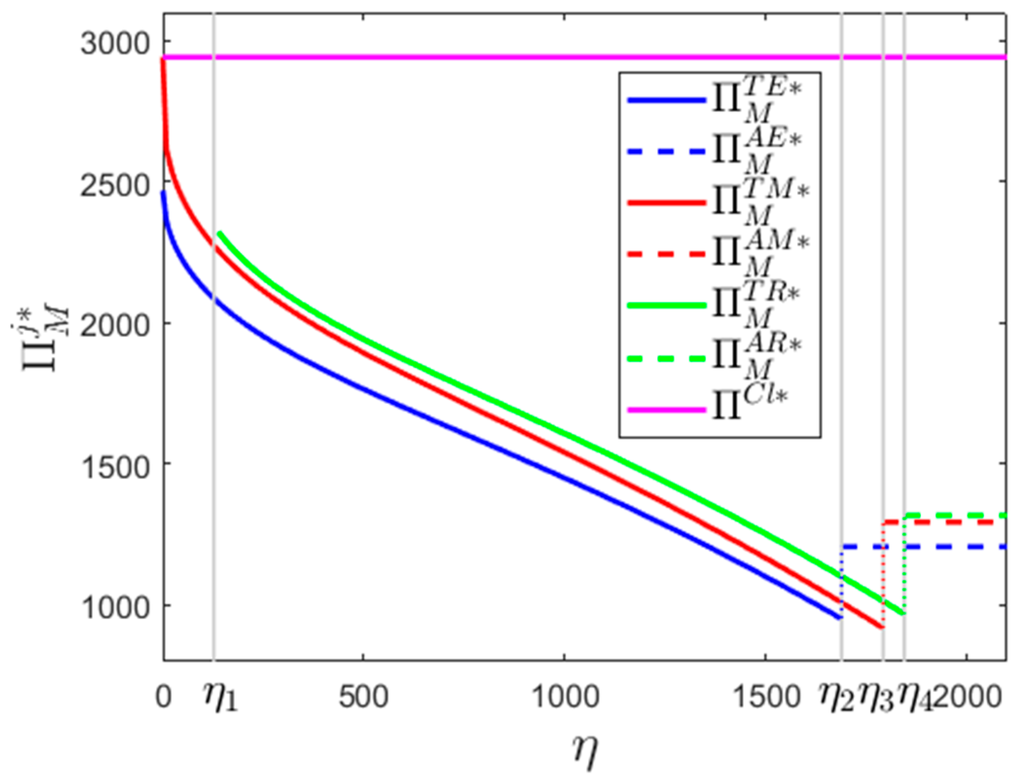
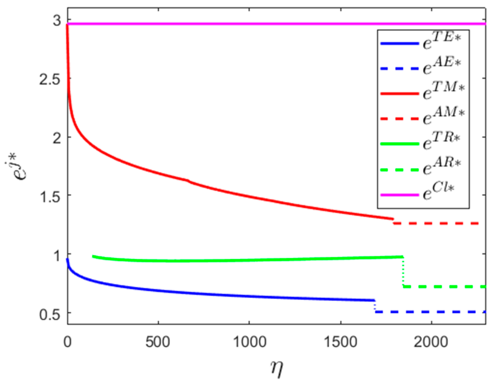
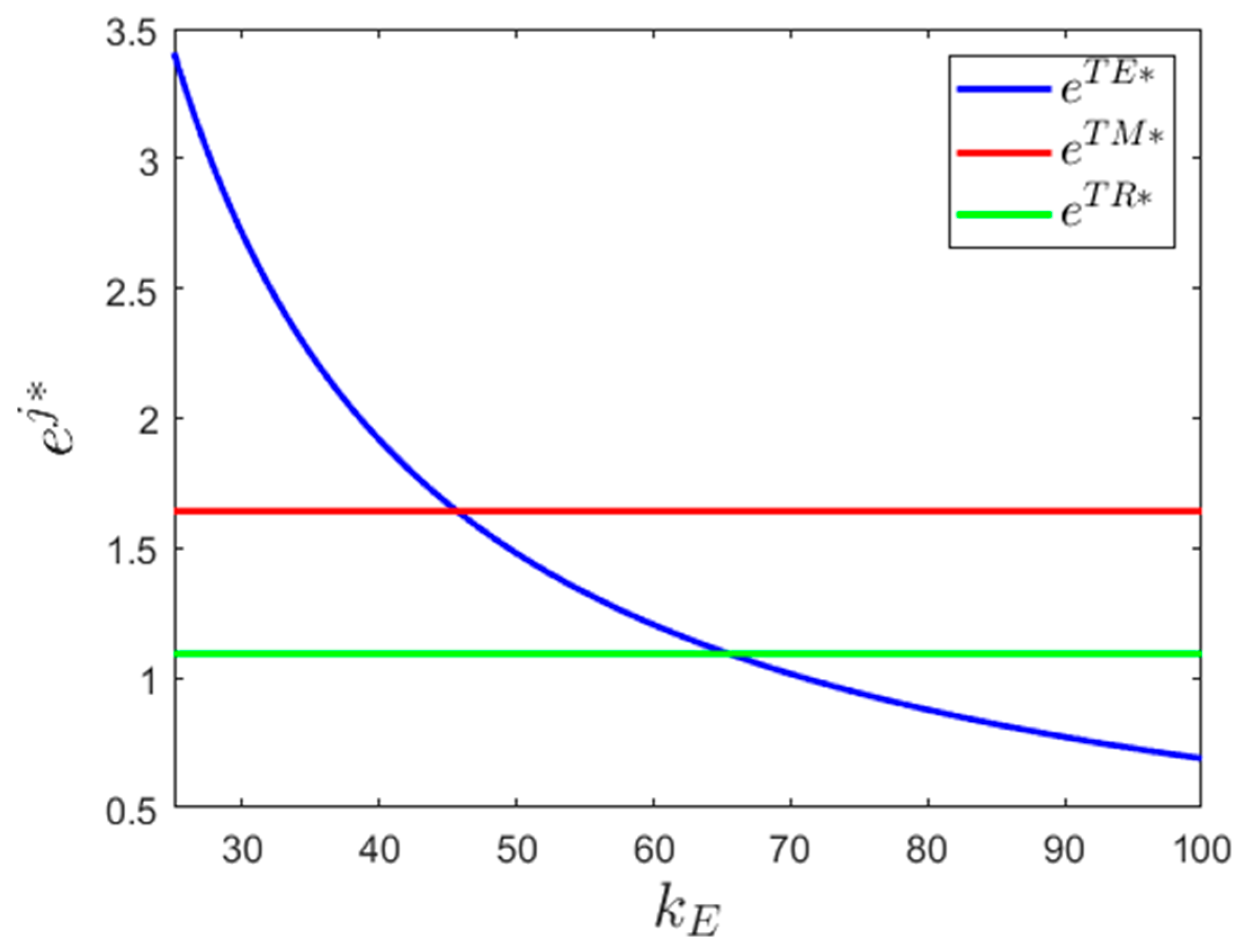
Given $k_E=100,\beta =0.8,{\alpha }_M=0.8,{\alpha }_R=0.8$, we first analyze the impacts of $\eta$ on the operation of the low-carbon supply chain system. Our main findings are as follows. First, trade credit finance brings economic and environmental benefits to the supply chain at the same time. In Figure 1 and Figure 2 the manufacturer’s CVaR utilities and the carbon emission reduction efforts in different modes increase with the decrease in the retailer’s initial capital amount. As we can see, ${\mathsf{\Pi }}_M^{Tl\ast }+{\mathsf{\Pi }}_R^{Tl\ast }+{\mathsf{\Pi }}_E^{Tl\ast }{|}_{l=E}>{\mathsf{\Pi }}_M^{Al\ast }+{\mathsf{\Pi }}_R^{Al\ast }+{\mathsf{\Pi }}_E^{Al\ast }{|}_{l=E}$ and $e_{}^{TM\ast }>e_{}^{AM\ast }$ are established when $\eta$ is sufficiently low. In particular, when $\eta$ decreases to 0, ${\mathsf{\Pi }}_M^{TM\ast }$ and $e_{}^{TM\ast }$ increase to ${\mathsf{\Pi }}_M^{CM\ast }$ and $e_{}^{CM\ast }$, respectively. These results are different to those in Wang et al. [22], reflecting the impact of an increase in decision variables on low-carbon supply chain operation.

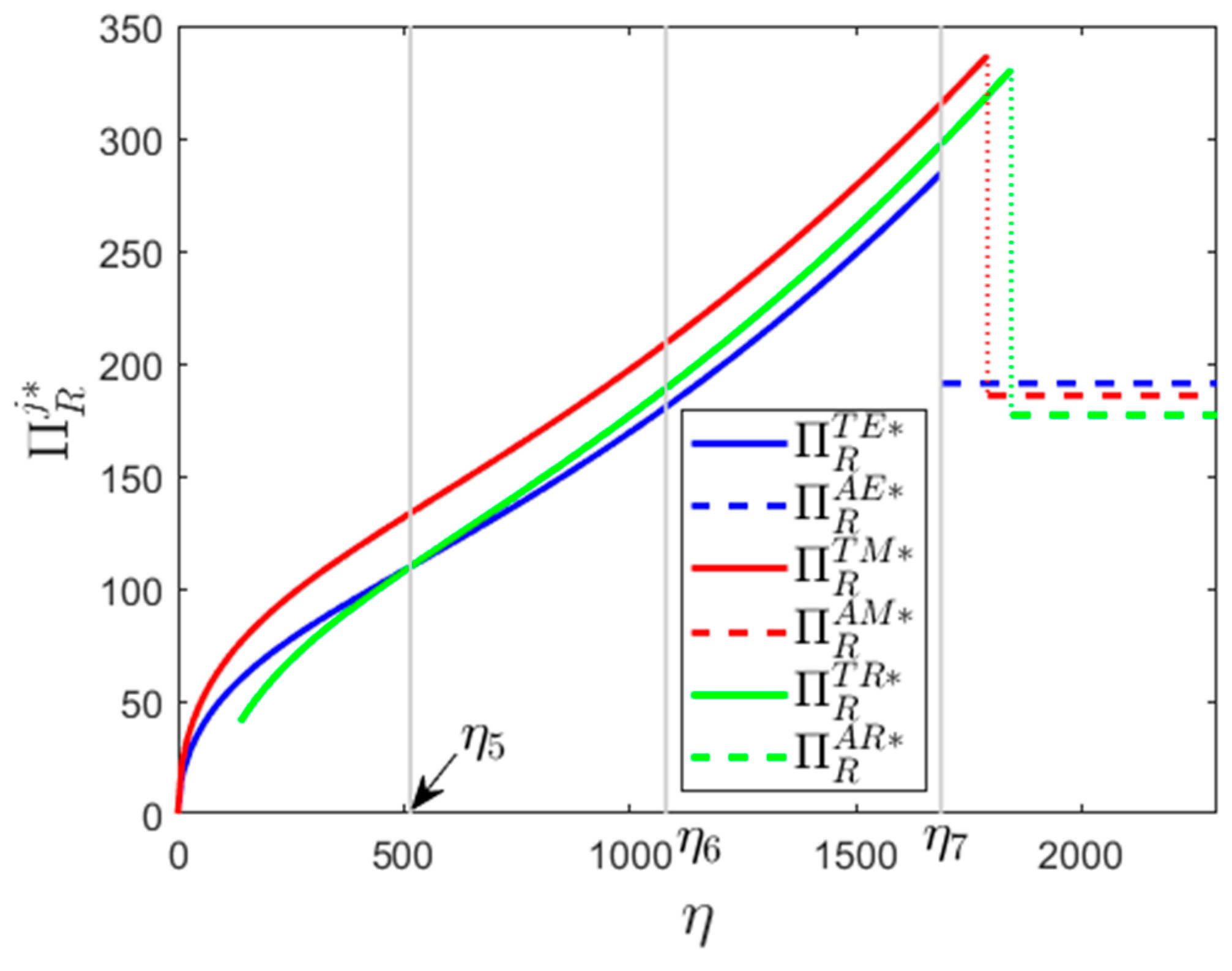
Second, as seen Figure 3 for the retailer’s perspective, trade credit finance can create value for the retailer when $\eta$ is in the middle position, e.g., when $\eta$ is in the $[{\eta }_6,{\eta }_7]$ interval in Mode E (${\mathsf{\Pi }}_R^{TE\ast }>{\mathsf{\Pi }}_R^{AE\ast }$ is established at this time). Nevertheless, excessive reliance on trade credit is detrimental to the retailer. As we can see, ${\mathsf{\Pi }}_R^{TM\ast }$, ${\mathsf{\Pi }}_R^{TE\ast }$, ${\mathsf{\Pi }}_R^{TR\ast }$ decrease with respect to the decrease of $\eta$. In particular, ${\mathsf{\Pi }}_R^{TM\ast }$ and ${\mathsf{\Pi }}_R^{TE\ast }$ both decrease to 0 when $\eta$ is reduced to 0. The retailer should use capital properly to maintain a higher income level.

Third, comparing the different carbon emission reduction modes, we can see that the optimal modes for the manufacturer are Mode TM, Mode TR, Mode AE, Mode AM, and Mode AR when $\eta$ is in $[0,{\eta }_1]$, $[{\eta }_1,{\eta }_2]$, $[{\eta }_2,{\eta }_3]$, $[{\eta }_3,{\eta }_4]$, and $[{\eta }_4,+\infty ]$, respectively. From the environmental perspective, it is always optimal for the manufacturer to conduct carbon emission reduction since $e_{}^{TM\ast }>e_{}^{TR\ast }>e_{}^{TE\ast }$ and $e_{}^{AM\ast }>e_{}^{AR\ast }>e_{}^{AE\ast }$ are always established. In the retailer’s perspective, the optimal carbon emission reduction modes are Mode TM, Mode TR, and Mode AE when $\eta$ is in $[0,{\eta }_3],[{\eta }_3,{\eta }_4],[{\eta }_4,+\infty ]$, respectively. Comparing Mode TR and Mode TE, we can see that Mode TE and Mode TR are dominant strategies for the retailer when $\eta \in [0,{\eta }_5]$ and $\eta \in [{\eta }_5,{\eta }_4]$, respectively. To sum up the above analysis, the retailer’s capital situation impacts the optimal decision of the carbon emission reduction mode selection.

The above analysis provides some managerial insights to allow managers to better manage the low-carbon supply chain. First, the carbon emission investor should increase the carbon emission reduction effort with respect to the decrease in the retailer’s initial capital amount. Second, trade credit contract should be adopted by the manufacturer to improve the economic and environmental benefits of the supply chain. Third, the retailer should use more initial capital when they participate in the trade credit contract. They should also appropriately reduce the amount of capital used when their initial capital amount is high enough, e.g., when $\eta$ is in the $[{\eta }_7,+\infty ]$. Fourth, the manufacturer should reasonably choose the carbon emission reduction mode according to the retailer’s initial capital amount. For example, they should implement carbon emission reduction by themselves when the retailer’s initial capital amount is low enough, e.g., $\eta \in [0,{\eta }_1]$. They should outsource the carbon emission reduction to the retailer when the retailer’s initial capital amount is in the middle position, e.g., $\eta \in [{\eta }_1,{\eta }_2]$. When the capital amount is in a higher position, e.g., $\eta \in [{\eta }_2,{\eta }_3]$, the manufacturer should outsource the carbon emission reduction to the ESCO.

6.2. Impacts of $k_E$

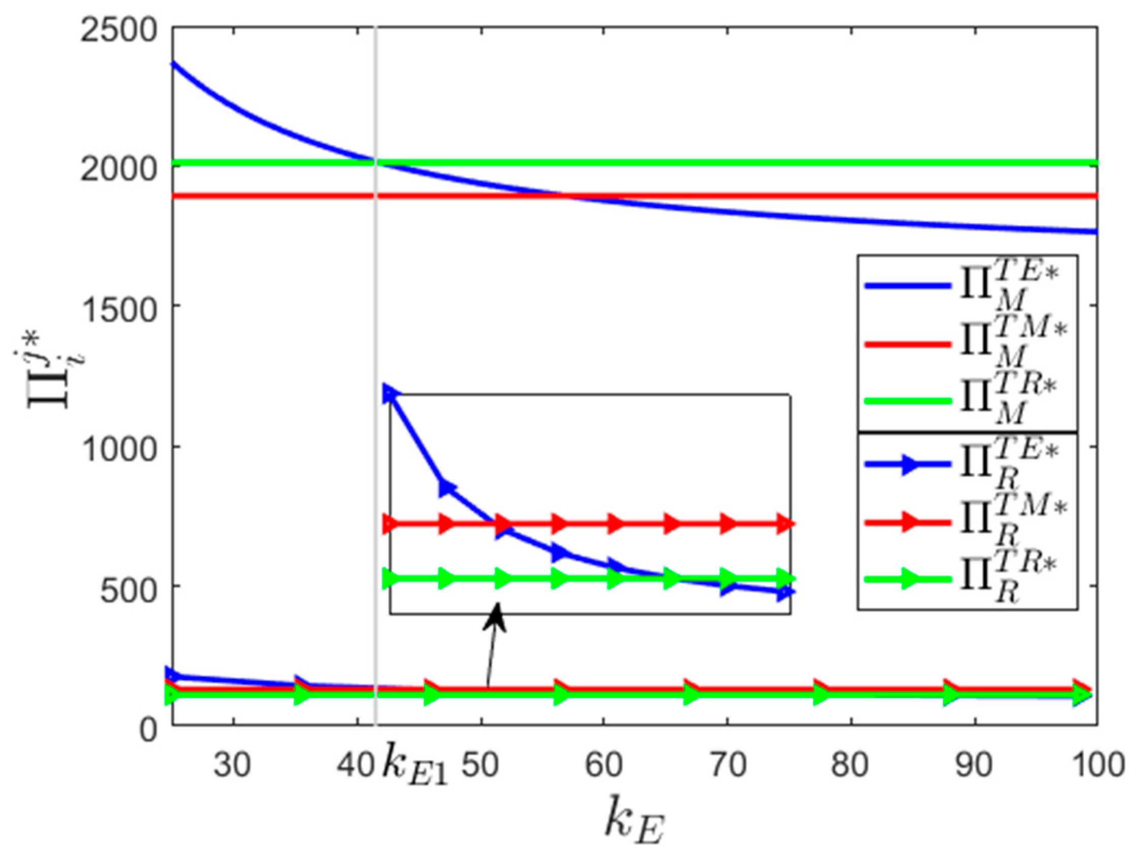
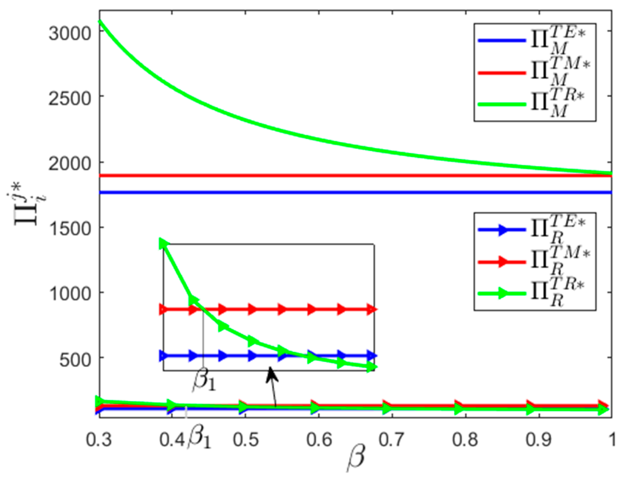
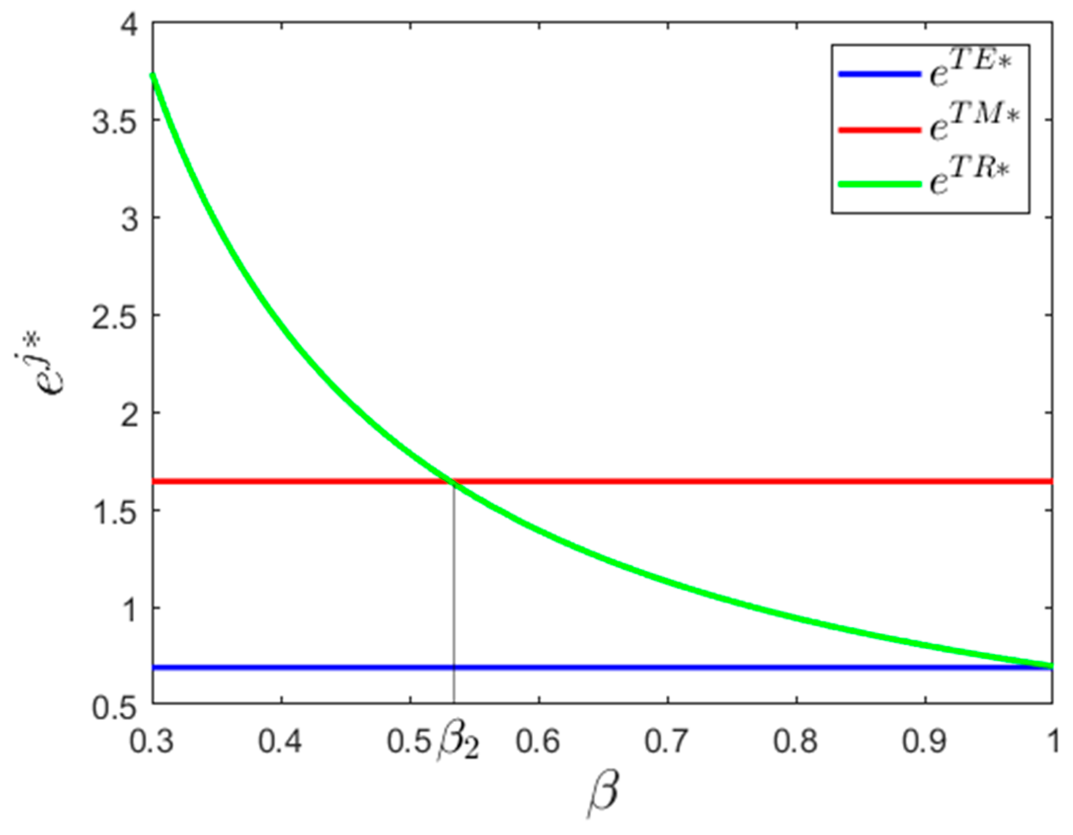
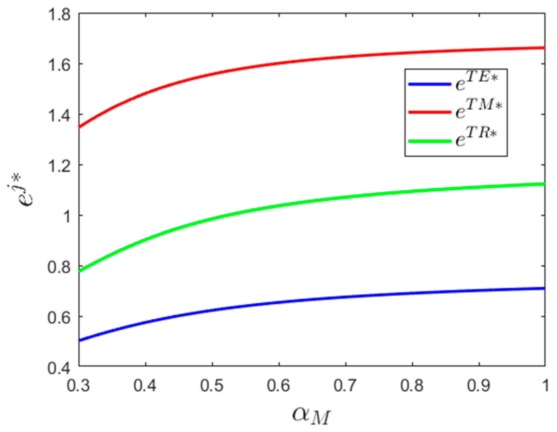
We assumed that the R&D investment cost scale economy coefficients $k_E,k_M,k_R$ are the same as in Section 6.1. In reality, the ESCO usually has a more professional level of carbon emission reduction than the manufacturer and the retailer. Therefore, the carbon emission reduction cost in Mode E is also lower than in Mode M and Mode R. That is, $k_E<\min \{k_M,k_R\}$. In the next section, we analyze the impacts of $k_E$ on the supply chain. We fixed $\beta =0.8,{\alpha }_M=0.8,{\alpha }_R=0.8,\eta =600$, and we perform a sensitivity analysis for $k_E$. In Figure 4 and Figure 5, we can see that ${\mathsf{\Pi }}_M^{TE\ast }$, ${\mathsf{\Pi }}_R^{TE\ast }$, and $e_{}^{TE\ast }$ are decreasing in $k_E$, and ${\mathsf{\Pi }}_M^{TE\ast }>\max \{{\mathsf{\Pi }}_M^{TM\ast },{\mathsf{\Pi }}_M^{TR\ast }\}$, ${\mathsf{\Pi }}_R^{TE\ast }>\max \{{\mathsf{\Pi }}_R^{TM\ast },{\mathsf{\Pi }}_R^{TR\ast }\}$, $e_{}^{TE\ast }>\max \{e_{}^{TM\ast },e_{}^{TR\ast }\}$ are synchronously established when $k_E<k_{E1}$, showing that ESCO carbon emission reduction can create both economic and environmental benefits for the supply chain and can create a win-win situation between the manufacturer and the retailer when $k_E$ is less than a critical threshold. The manufacturer should adopt Mode E when the ESCO’s carbon emission reduction cost is sufficiently low compared with that of other modes. However, ${\mathsf{\Pi }}_M^{TE\ast }<\min \{{\mathsf{\Pi }}_M^{TM\ast },{\mathsf{\Pi }}_M^{TR\ast }\}$, ${\mathsf{\Pi }}_R^{TE\ast }<\max \{{\mathsf{\Pi }}_R^{TM\ast },{\mathsf{\Pi }}_R^{TR\ast }\}$, $e_{}^{TE\ast }<\max \{e_{}^{TM\ast },e_{}^{TR\ast }\}$ are synchronously established when $k_E$ is high enough, e.g., $k_E=k_M=k_R$. The cost advantage of Mode E no longer exists.

6.3. Impacts of $\beta$

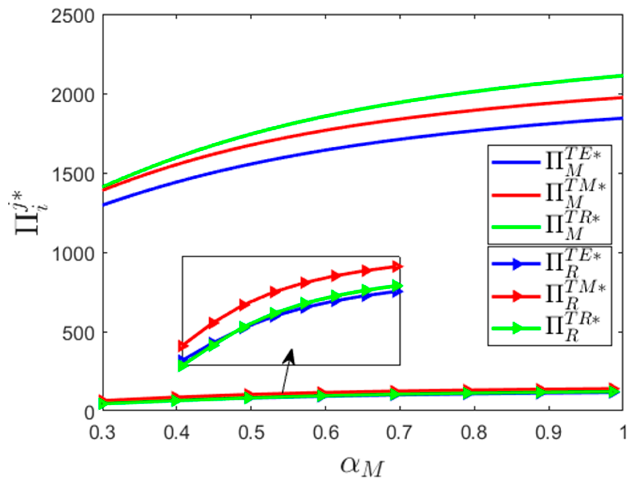
Let $k_E=100,{\alpha }_M=0.8,{\alpha }_R=0.8,\eta =600$; we further analyze the impacts of the cash investment ratio of carbon emission reduction R&D $\beta$. Figure 6 and Figure 7 show that the manufacturer and the retailer’s CVaR utilities in Mode TR—${\mathsf{\Pi }}_M^{TR\ast }$, ${\mathsf{\Pi }}_R^{TR\ast }$, and the carbon emission reduction effort $e_{}^{TR\ast }$ increases with decreasing $\beta$. In particular, when $\beta <{\beta }_1$, ${\mathsf{\Pi }}_M^{TR\ast }>\max \{{\mathsf{\Pi }}_M^{TM\ast },{\mathsf{\Pi }}_M^{TE\ast }\}$, ${\mathsf{\Pi }}_R^{TR\ast }>\max \{{\mathsf{\Pi }}_R^{TM\ast },{\mathsf{\Pi }}_R^{TE\ast }\}$, $e_{}^{TR\ast }>\max \{e_{}^{TM\ast },e_{}^{TE\ast }\}$ are synchronously established. That is, Pareto improvement of the economic and environmental benefits is realized with the decrease in $\beta$. Mode TR becomes the optimal carbon emission reduction mode for the manufacturer and the retailer at the same time when $\beta \in [0,{\beta }_1]$. Thus, it is clear to see that the capital-constrained retailer that undertakes the carbon emission reduction commitment can create great value for the supply chain. The manufacturer should outsource the carbon emission to the retailer when the cash investment ratio of carbon emission reduction R&D $\beta$ is low enough. However, ${\mathsf{\Pi }}_R^{TR\ast }<\min \{{\mathsf{\Pi }}_R^{TM\ast },{\mathsf{\Pi }}_R^{TE\ast }\}$ is established when $\beta$ is high enough. At this time, undertaking the carbon emission reduction task is detrimental to the retailer self.

6.4. Impacts of ${\alpha }_M,{\alpha }_R$

Most of the studies related to risk attitude, such as Wu et al. [47] and Ozgun et al. [51], have indicated that the retailer’s order decision and their expected utility is increasing in ${\alpha }_R$. However, they do not know how to make a carbon emission reduction decision according to the decision-makers’ risk attitude. We then analyze the impacts of the decision maker’s risk attitude on the low carbon supply chain operation. Fixing $k_E=100,\beta =0.8,{\alpha }_R=0.8,\eta =600$, we first perform sensitivity analysis on ${\alpha }_M$. In Figure 8 and Figure 9, regardless of the type of carbon emission mode, the manufacturer and the retailer’s CVaR utilities and the carbon emission reduction effort all decrease with respect to the decrease in ${\alpha }_M$ because the more risk-averse manufacturer is more likely to make a conservative decision, improving the wholesale price, which leads to the increase in double marginalization and the efficiency loss of the supply chain. Thus, the manufacturer’s risk-averse behavior is detrimental to the supply chain.

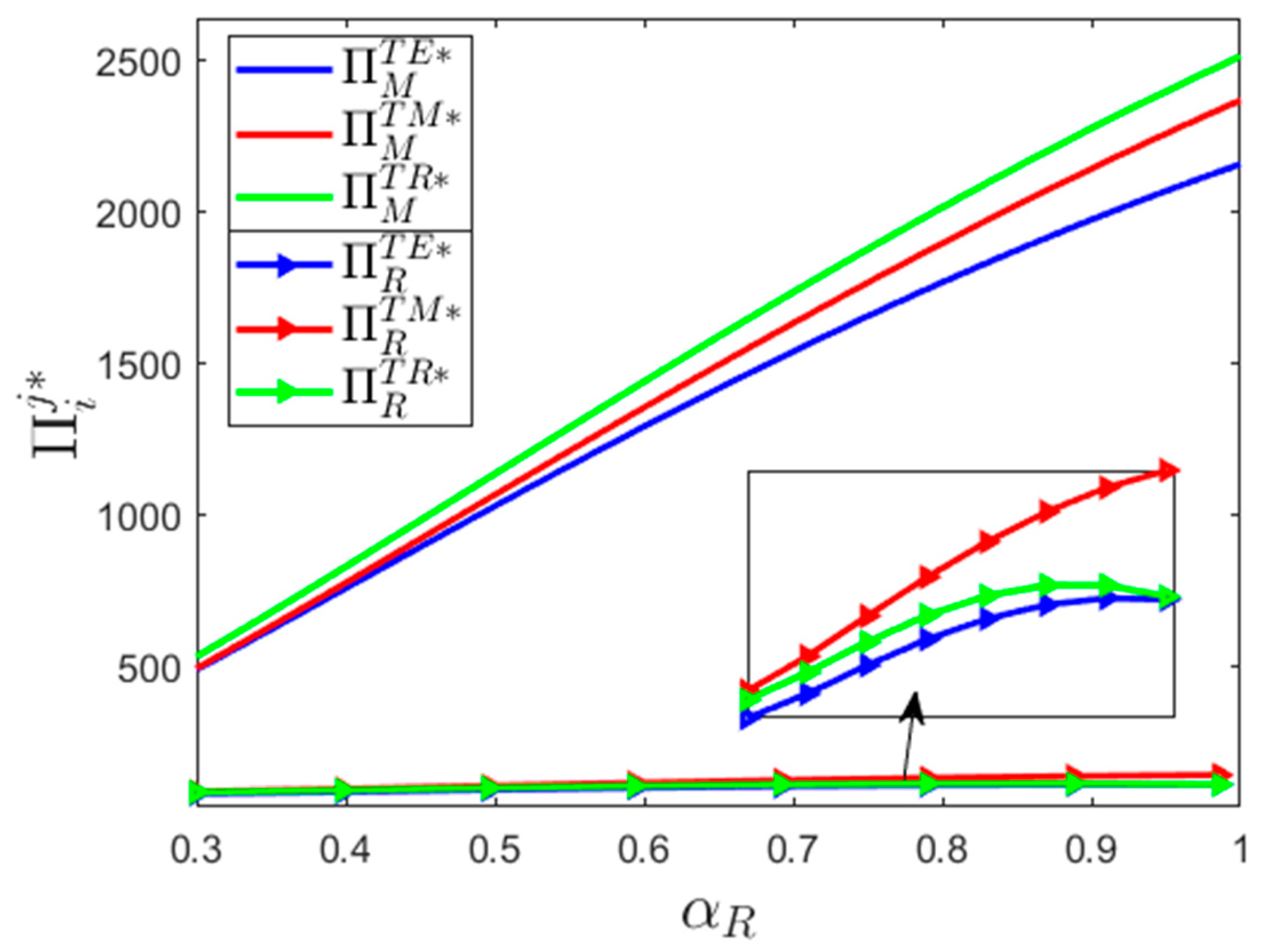
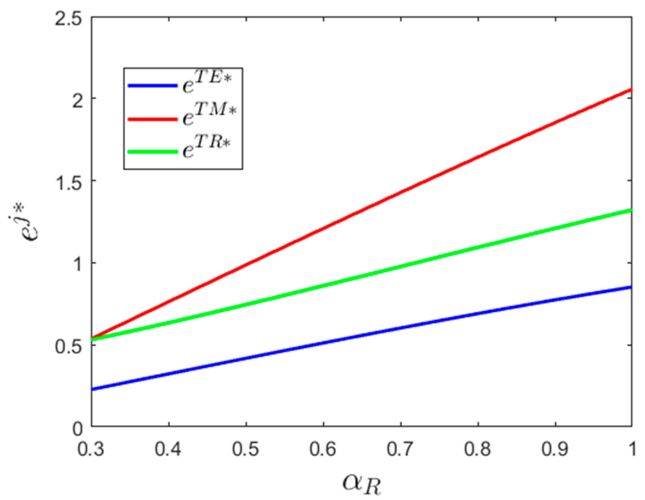
Fixing $k_E=100,\beta =0.8,{\alpha }_M=0.8,\eta =600$, we further analyze the retailer’s risk attitude. As we can see in Figure 10 and Figure 11, influenced by the risk-averse retailer’s conservative order decision behavior, ${\mathsf{\Pi }}_M^{Tl\ast }$, ${\mathsf{\Pi }}_R^{Tl\ast }{|}_{l\ne R}$, and $e_{}^{Tl\ast }$ are all decreasing with respect to the decrease in ${\alpha }_R$. The ${\mathsf{\Pi }}_R^{TR\ast }$ is first increasing and then decreasing in ${\alpha }_R$ because with the decrease in ${\alpha }_R$, the manufacturer chooses to decrease the wholesale price to prevent the adverse effect caused by the risk-averse retailer’s negative ordering behavior, which can have positive effects for the retailer. However, the manufacturer and retailer’s risk-averse behavior is not conducive to the development of carbon emission reduction.

The above analysis indicates that the decision-makers’ risk-aversion behavior is detrimental to both economics and the environment. The carbon emission reduction investor should decrease the carbon emission reduction effort with respect to the increase of the decision-makers’ risk aversion degree.

7. Conclusions

The need for low-carbon development has become a social consensus. Increasing numbers of enterprises implement carbon emission reduction strategies to meet the needs of the consumer market and to practice social responsibility. Manufacturer-led, retailer-led, and ESCO-led mechanisms are three mainstream strategies for realizing carbon emission reduction of the supply chain. We explore the optimal carbon emission reduction strategy by comparing these three reduction mechanisms. The impacts of capital constraint and risk aversion on the operation, decision-making, mode selection, and coordination of the low carbon supply chain are also analyzed.

We developed Stackelberg game models to describe and compare three different carbon emission reduction modes. We discussed the impacts of capital constraint and risk aversion on the operation of the low-carbon supply chain by analyzing the parameters’ sensitivity. The major findings can be summarized as follows. First, the total utility and carbon emission effort level are higher in Mode T than that in the traditional Mode A. That is, trade credit can create great benefits for both the economy and the environment. Second, the dominant carbon emission reduction mechanism of the manufacturer changes as the retailer’s initial capital amount changes. That is, capital constraint greatly impacts the carbon emission reduction mode selection. Third, the manufacturer’s expected utility in Mode E (Mode R) is higher than that in other modes when the ESCO’s carbon emission reduction operation cost advantage (the retailer’s initial capital amount, carbon emission reduction investment cost ratio) is (are) sufficiently high (low). Fourth, overall, decision-makers’ risk aversion is detrimental to both the economic and environmental development of the supply chain. Fifth, supply chain coordination can realize the Pareto improvement of the low-carbon supply chain.

Reasonable carbon emission reduction decisions, low-carbon supply chain coordination, and carbon emission reduction mode selection can increase the operational efficiency of the low-carbon supply chain. This research provides a theoretical basis for decision-makers to implement low-carbon supply chain management from the perspective of the interface between operation and finance. The results have positive driving significance for the development of a sustainable supply chain. We summarize main managerial insights and answer the four research questions proposed in Section 1 as follows. First, trade credit contracts should be promoted for use in commercial transactions to improve the operational efficiency of the low-carbon supply chain. Second, Proposition 1 to Proposition 6 provide decision references for decision-makers to make joint operation, finance, and environment decisions optimally. In addition, the capital amount and risk-aversion degree are two key factors affecting the carbon emission reduction decision. Carbon emission reduction investors should increase (decrease) the carbon emission reduction effort with respect to the decrease (increase) of the retailer’s initial capital amount (decision-makers’ risk-aversion degree). This is also the answer to question (1) in Section 1. Third, decision-makers should make appropriate adjustments to the carbon emission reduction mode selection decision according to the changes of key parameters. When the ESCO’s carbon emission reduction operation cost advantage (retailer’s initial capital amount, carbon emission reduction investment cost ratio) is (are) sufficiently high (low), it is optimal for the manufacturer to outsource the carbon emission directly to the ESCO (retailer). These results answer question (2) in the Introduction. Fourth, managers should coordinate the supply chain through proper use of contracts to realize the Pareto improvement of the supply chain members. The contracts designed in this paper (Proposition 10–Proposition 12) can realize the coordination of the risk-neutral, risk-averse, capital-adequate, and capital-constrained low-carbon supply chains. This is the answer to question (3).

There are also some limitations and valuable research directions that leave room for future research. First, the information is assumed as shared knowledge for enterprises in this paper. The information asymmetry scenario can be further explored. Second, the sales market and carbon emission reduction market are all monopolies in our setting. The exploration of the impacts of market competition on the comparison of different carbon emission reduction modes is the direction of the ongoing work for future research. Third, only trade credit finance is considered in this paper. We can further discuss the other financing modes, such as equity finance, internet finance, and logistics finance, and continue to perform more expansibility research in the future.

References

- Wang, Z.; Wang, C. How carbon offsetting scheme impacts the duopoly output in production and abatement: Analysis in the context of carbon cap-and trade. J. Clean. Prod. 2015, 103, 715–723. [Google Scholar] [CrossRef]
- Nouira, M.; Hammami, R.; Frein, Y.; Temponi, C. Design of forward supply chains: Impact of a carbon emissions-sensitive demand. Int. J. Prod. Econ. 2016, 173, 80–98. [Google Scholar] [CrossRef]
- Zhang, L.; Wang, J.; You, J. Consumer environmental awareness and channel coordination with two substitutable products. Eur. J. Oper. Res. 2015, 241, 63–73. [Google Scholar] [CrossRef]
- Cohen, M.; Vandenbergh, M. The potential role of carbon labeling in a green economy. Energy Econ. 2012, 34, 53–63. [Google Scholar] [CrossRef]
- Ji, J.; Zhang, Z.; Yang, L. Comparisons of initial carbon allowance allocation rules in an O2O retail supply chain with the cap-and-trade regulation. Int. J. Prod. Econ. 2017, 187, 68–84. [Google Scholar] [CrossRef]
- Panda, S.; Modak, N.; Cardenas-Barron, L. Coordinating a socially responsible closed-loop supply chain with product recycling. Int. J. Prod. Econ. 2017, 188, 11–21. [Google Scholar] [CrossRef]
- Zu, Y.; Chen, L.; Fan, Y. Research on low-carbon strategies in supply chain with environmental regulations based on differential game. J. Clean. Prod. 2018, 177, 527–546. [Google Scholar] [CrossRef]
- Stuart, E.; Larsen, P.; Goldman, C.; Gilligan, D. A method to estimate the size and remaining market potential of the U.S. ESCO (energy service company) industry. Energy 2014, 77, 362–371. [Google Scholar] [CrossRef]
- Deng, X.; Zheng, S.; Xu, P.; Zhang, X. Study on dissipative structure of China’s building energy service industry system based on brusselator model. J. Clean. Prod. 2017, 150, 112–122. [Google Scholar] [CrossRef]
- Xu, J.; Chen, Y.; Bai, Q. A two-echelon sustainable supply chain coordination under cap-and-trade regulation. J. Clean. Prod. 2016, 135, 42–56. [Google Scholar] [CrossRef]
- Xu, X.; He, P.; Xu, H.; Zhang, Q. Supply chain coordination with green technology under cap-and-trade regulation. Int. J. Prod. Econ. 2017, 183, 433–442. [Google Scholar] [CrossRef]
- Hua, G.; Cheng, T.; Wang, S. Managing carbon footprints in inventory management. Int. J. Prod. Econ. 2011, 132, 178–185. [Google Scholar] [CrossRef]
- Benjaafar, S.; Li, Y.; Daskin, M. Carbon footprint and the management of supply chains: Insights from simple models. IEEE Trans. Autom. Sci. Eng. 2013, 10, 99–116. [Google Scholar] [CrossRef]
- Du, S.; Hu, L.; Song, M. Production optimization considering environmental performance and preference in the cap-and-trade system. J. Clean. Prod. 2016, 112, 1600–1607. [Google Scholar] [CrossRef]
- Du, S.; Zhu, J.; Jiao, H.; Ye, W. Game-theoretical analysis for supply chain with consumer preference to low carbon. Int. J. Prod. Res. 2015, 53, 3753–3768. [Google Scholar] [CrossRef]
- Xia, L.; Guo, T.; Qin, J.; Yue, X.; Zhu, N. Carbon emission reduction and pricing policies of a supply chain considering reciprocal preferences in cap-and-trade system. Ann. Oper. Res. 2018, 268, 149–175. [Google Scholar] [CrossRef]
- Wang, X.; Xue, M.; Xing, L. Analysis of carbon emission reduction in a dual-channel supply chain with cap-and-trade regulation and low-carbon preference. Sustainability 2018, 10, 580. [Google Scholar]
- He, R.; Xiong, Y.; Lin, Z. Carbon emissions in a dual channel closed loop supply chain: The impact of consumer free riding behavior. J. Clean. Prod. 2016, 134, 384–394. [Google Scholar] [CrossRef]
- Yang, L.; Zhang, Q.; Ji, J. Pricing and carbon emission reduction decisions in supply chains with vertical and horizontal cooperation. Int. J. Prod. Econ. 2017, 191, 286–297. [Google Scholar] [CrossRef]
- Zhou, Y.; Bao, M.; Chen, X.; Xu, X. Co-op advertising and emission reduction cost sharing contracts and coordination in low-carbon supply chain based on fairness concerns. J. Clean. Prod. 2016, 133, 402–413. [Google Scholar] [CrossRef]
- Roshchank, V.; Evans, M. Scaling up the energy service company business: Market status and company feedback in the Russian federation. J. Clean. Prod. 2016, 112, 3905–3914. [Google Scholar] [CrossRef]
- Wang, W.; Chen, W.; Liu, B. Manufacturing/remanufacturing decisions for a capital-constrained manufacturer considering carbon emission cap and trade. J. Clean. Prod. 2017, 140, 1118–1128. [Google Scholar] [CrossRef]
- Cao, E.; Yu, M. Trade credit financing and coordination for an emission-dependent supply chain. Comput. Ind. Eng. 2018, 119, 50–62. [Google Scholar] [CrossRef]
- Gupta, D.; Wang, L. A stochastic inventory model with trade credit. Manuf. Serv. Oper. Manag. 2009, 11, 4–18. [Google Scholar] [CrossRef]
- Xu, X.; Meng, Z.; Shen, R. A tri-level programming model based on conditional value-at-risk for three-stage supply chain management. Comput. Ind. Eng. 2013, 6, 470–475. [Google Scholar] [CrossRef]
- Koller, T.; Lovallo, D.; Williams, Z. Overcoming a bias against risk. Tech. Rep. 2012, 4, 15–17. Available online: https://www.mendeley.com/research-papers/overcoming-bias-against-risk/ (accessed on 1 August 2012).
- Buzacott, J.; Zhang, R. Inventory management with asset-based financing. Manag. Sci. 2014, 50, 1274–1292. [Google Scholar] [CrossRef]
- Chao, X.; Chen, J.; Wang, S. Dynamic inventory management with financial. Nav. Res. Logist. 2008, 55, 758–765. [Google Scholar] [CrossRef]
- Protopappa-Sieke, M.; Seifert, R. Interrelating operational and financial performance measurements in inventory control. Eur. J. Oper. Res. 2010, 204, 439–448. [Google Scholar] [CrossRef]
- Yang, A.; Birge, J.; Parker, R. The supply chain effects of bankruptcy. Manag. Sci. 2015, 61, 2320–2338. [Google Scholar] [CrossRef]
- Feng, Y.; Mu, Y.; Hu, B.; Kumar, A. Commodity options purchasing and credit financing under capital constraint. Int. J. Prod. Econ. 2014, 153, 230–237. [Google Scholar] [CrossRef]
- Yan, X.; Wang, Y. A newsvendor model with capital constraint and demand forecast update. J. Clean. Prod. 2014, 52, 5021–5040. [Google Scholar] [CrossRef]
- Sarkar, B. Mathematical and analytical approach for the management of defective items in a multi-stage production system. J. Clean. Prod. 2019, 218, 896–919. [Google Scholar] [CrossRef]
- Luo, J.; Zhang, Q. Trade credit: A new mechanism to coordinate supply chain. Oper. Res. Lett. 2012, 40, 278–384. [Google Scholar] [CrossRef]
- Chen, X.; Wang, A. Trade credit contract with limited liability in the supply chain with budget constraints. Ann. Oper. Res. 2012, 196, 153–165. [Google Scholar] [CrossRef]
- Zhang, Q.; Dong, M.; Luo, J. Supply chain coordination with trade credit and quantity discount incorporating default risk. Int. J. Prod. Econ. 2014, 153, 352–360. [Google Scholar] [CrossRef]
- Wu, D.; Zhang, B.; Opher, B. A trade credit model with asymmetric competing retailers. Prod. Oper. Manag. 2018. [Google Scholar] [CrossRef]
- Jing, B.; Chen, X.; Cai, G. Equilibrium financing in a distribution channel with capital constraint. Prod. Oper. Manag. 2012, 21, 1090–1101. [Google Scholar] [CrossRef]
- Cai, G.; Chen, X.; Xiao, Z. The roles of bank and trade credits: Theoretical analysis and empirical evidence. Prod. Oper. Manag. 2014, 23, 583–598. [Google Scholar] [CrossRef]
- Kouvelis, P.; Zhao, W. Who should finance the supply chain? Impact of credit ratings on supply chain decisions. Manuf. Serv. Oper. Manag. 2018, 20, 19–35. [Google Scholar] [CrossRef]
- Tang, C.; Yang, A.; Wu, J. Sourcing from suppliers with financial constraints and performance risk. Manuf. Serv. Oper. Manag. 2018, 20, 70–84. [Google Scholar] [CrossRef]
- Rabe, M.; Streimikiene, D.; Bilan, Y. The concept of risk and possibilities of application of mathematical methods in supporting decision making for sustainable energy development. Sustainability 2019, 11, 1018. [Google Scholar] [CrossRef]
- Alexander, G.; Baptista, A. A comparison of VaR and CVaR constraints on portfolio selection with the Mean-Variance model. Manag. Sci. 2004, 50, 1261–1273. [Google Scholar] [CrossRef]
- Gotoh, J.; Takano, Y. Newsvendor solutions via conditional value-at-risk minimization. Eur. J. Oper. Res. 2007, 179, 80–96. [Google Scholar] [CrossRef]
- Chen, Y.; Xu, M.; Zhang, Z. A risk-averse newsvendor model under the CVaR decision criterion. Oper. Res. 2009, 57, 1040–1044. [Google Scholar] [CrossRef]
- Wu, M.; Zhu, S.; Teunter, R. The risk-averse newsvendor problem with random capacity. Eur. J. Oper. Res. 2013, 231, 328–336. [Google Scholar] [CrossRef]
- Wu, M.; Zhu, S.; Teunter, R. A risk-averse competitive newsvendor problem under the CVaR criterion. Int. J. Prod. Econ. 2014, 156, 13–23. [Google Scholar] [CrossRef]
- Qiu, R.; Shang, J.; Huang, X. Robust inventory decision under distribution uncertainty: A CVaR-based optimization approach. Int. J. Prod. Econ. 2014, 153, 13–23. [Google Scholar] [CrossRef]
- Xue, W.; Ma, L.; Shen, H. Optimal inventory and hedging decisions with CVaR consideration. Int. J. Prod. Econ. 2015, 162, 70–82. [Google Scholar] [CrossRef]
- Yang, L.; Xu, M.; Yu, G.; Zhang, H. Supply chain coordination with CVaR Criterion. Asia Pac. J. Oper. Res. 2009, 26, 135–160. [Google Scholar] [CrossRef]
- Ozgun, C.; Chen, Y.; Li, J. Customer and retailer rebates under risk aversion. Int. J. Prod. Econ. 2011, 133, 736–750. [Google Scholar]
- Li, B.; Hou, P.; Chen, P. Pricing strategy and coordination in a dual channel supply chain with a risk-averse retailer. Int. J. Prod. Econ. 2016, 178, 154–168. [Google Scholar] [CrossRef]
- Chen, X.; Shum, S.; Simchi, D. Stable and coordinating contracts for a supply chain with multiple risk-averse suppliers. Prod. Oper. Manag. 2014, 23, 379–392. [Google Scholar] [CrossRef]