Improving the Life Cycle Impact Assessment of Metal Ecotoxicity: Importance of Chromium Speciation, Water Chemistry, and Metal Release

Abstract

Investigations of metal ecotoxicity in life cycle assessment (LCA) and life cycle impact assessment (LCIA) are becoming important tools for evaluating the environmental impact of a product or process. There is, however, improvement needed for LCIA of metal ecotoxicity in order to make this assessment more relevant and robust. In this work, three issues within the LCIA of metal ecotoxicity are investigated, mainly focusing on topics related to stainless steel manufacturing. The first issue is the importance of considering regional water chemistry when constructing the characterization factor (CF). A model freshwater of relevance for stainless steel manufacturing in a region of Sweden was created with chemistry different from available options. The second issue is related to the lack of consideration on changes in speciation of Cr(VI) in freshwater for a given emission, as Cr(VI) to some extent will be reduced to Cr(III). Two new options are suggested based on relationships between the Cr(VI)–total Cr ratio as a way to improve the relevancy of LCIA for Cr(VI) in freshwater. The last issue is how to treat metal release from slags in LCIA. Metal release from slags was shown to vary significantly between different ways of modelling slag emissions (differences in total metal content, slag leaching tests, estimated emissions to groundwater).

1. Introduction

Life cycle assessment (LCA) is increasingly used to investigate the environmental impact of products and processes, including stainless steel production [1]. The method accounts for the environmental impact during the entire life cycle, from the cradle to the grave [2,3,4]. According to ISO standards 14,040 [5] and 14,044 [6] regarding LCA, relevant environmental aspects should be considered both in the data inventory phase and in the impact assessment. The assessment is based on data collected from the life cycle inventory (LCI) on e.g. resources, energy, and emissions to water and air. A life cycle impact assessment (LCIA) of the environmental impact is based on data from this inventory in which a characterization factor (CF) is applied to the emission of interest to translate it to a potential environmental impact, including metal emissions translated into ecotoxicological impact [7]. Work is currently ongoing that aims to harmonize ecotoxicity characterization in LCIA [8,9].

Metals are dispersed to varying extents from several different processes during alloy manufacturing and from products during their service lives, for example metal release from constructions, metals in process water released to freshwater, and the diffuse metal release (leaching) from disposal of slags and landfills [10]. Previous studies have shown that both improved inventory data and improved methods for the assessment of ecotoxicological impact are needed to increase the relevance and accuracy of the assessment of metals leaching from slags, compared with data today available in USEtox (the consensus method for toxicity in LCIA) [11,12,13].

This study proposes a strategy to improve the accuracy and relevance of the LCIA with respect to metal-induced ecotoxicity of metals emitted/dispersed from slag deposits obtained as a direct consequence of stainless steel production. The metals in focus include nickel (Ni) and chromium (Cr) as they are of more environmental concern due to their toxic properties at certain conditions compared with other alloying metals such as iron (Fe) and molybdenum (Mo) [14]. The scope is further narrowed by considering only the freshwater compartment, but the same kind of issues when evaluating the ecotoxicological impact described above (inventory, methods for assessment) also translates to the marine and soil compartments [15,16].

The first aim of this study is to use the diffusive gradient in thin-films (DGT) technique to assess the labile metal fraction and estimate bioavailability factors (BF) for Cr(VI), Cr(III), and Ni in a model freshwater relevant for regions with stainless steel production in Sweden. These factors are compared with results of the Windermere humic acid model (WHAM) and the Visual MINTEQ theoretical modelling tools to assess the bioavailable metal fraction and partitioning coefficients [17]. Complete CFs are constructed using a framework outlined elsewhere [18], and compared with default CFs in USEtox as well as with other regional CFs. The use of DGT to assess the bioavailable metal fraction in freshwater is especially important for Cr(VI) due to a deficit in available CFs in LCIA.

The second aim of this work is to consider changes in oxidation state of Cr in freshwater in LCIA. Presently in USEtox, an emission of Cr(VI) is treated as it will remain in the same oxidation state independent of environmental interactions. Changes in Cr speciation are, however, very important to consider as the toxicity of Cr(VI) in general is much higher compared with Cr(III) [19]. It is well established that an emission of Cr(VI) at least to some extent will be reduced to Cr(III) upon entry into freshwater [20]. This study evaluates how different scenarios for Cr(VI) reduction kinetics influence the assessment of its ecotoxicity in LCIA. These scenarios are compared with the default way of treating Cr(VI) emissions in USEtox today in which no Cr transformation in speciation is considered.

The third aim is to determine metals release (leaching) from slags sampled stainless steel production sites. The use of by-products, waste material, and secondary raw materials such as slags from stainless steel manufacturing are of large importance in relation to ambitions of a circular economy. Such a use of industrial residues can contribute to the reduction of the overall environmental impact, both by considering mitigating negative impact from landfills and by enabling positive impact from use of secondary raw materials in construction. In such cases and in general, it is crucial that the LCIA of slags should be relevant and robust [21]. A strategy on how to facilitate such an analysis is given in this study. This is performed by means of DGT (bioavailable metal fraction) and applying the generated CFs for the model freshwater. These findings are compared with results using default CFs in USEtox and default slag leaching data for Cr in Ecoinvent (a life cycle inventory database) [11,22]. The hypothesis is that DGT measurements can provide a more realistic data and a relatively easy way to estimate the leaching of metals from slags compared with existing data in the Ecoinvent database, version 3 [23], often used in LCIA.

2. Materials and Methods

An overview of the strategy of this study is given in Figure 1 and described in the more detail in the sections below. In this study, we constructed CFs for Cr(VI), Cr(III) and Ni in a model freshwater in order to compare with default factors used in LCIA. The novel approach takes into account the reduction of Cr(VI) in freshwater, generates data for release of metals from slags, and applies the obtained CFs to the latter data. This is done using equilibrium modelling as well as DGT measurements to estimate the bioavailable metal fraction (labile fraction). Two different scenarios were constructed to take into account the effect of changes in redox state of Cr(VI), which also result in new CFs. We have in addition investigated the fraction of bioavailable metal leaching from slags from stainless production and how it influences the LCIA assessment compared with the current default approach using leaching data from slags available in the Ecoinvent database.

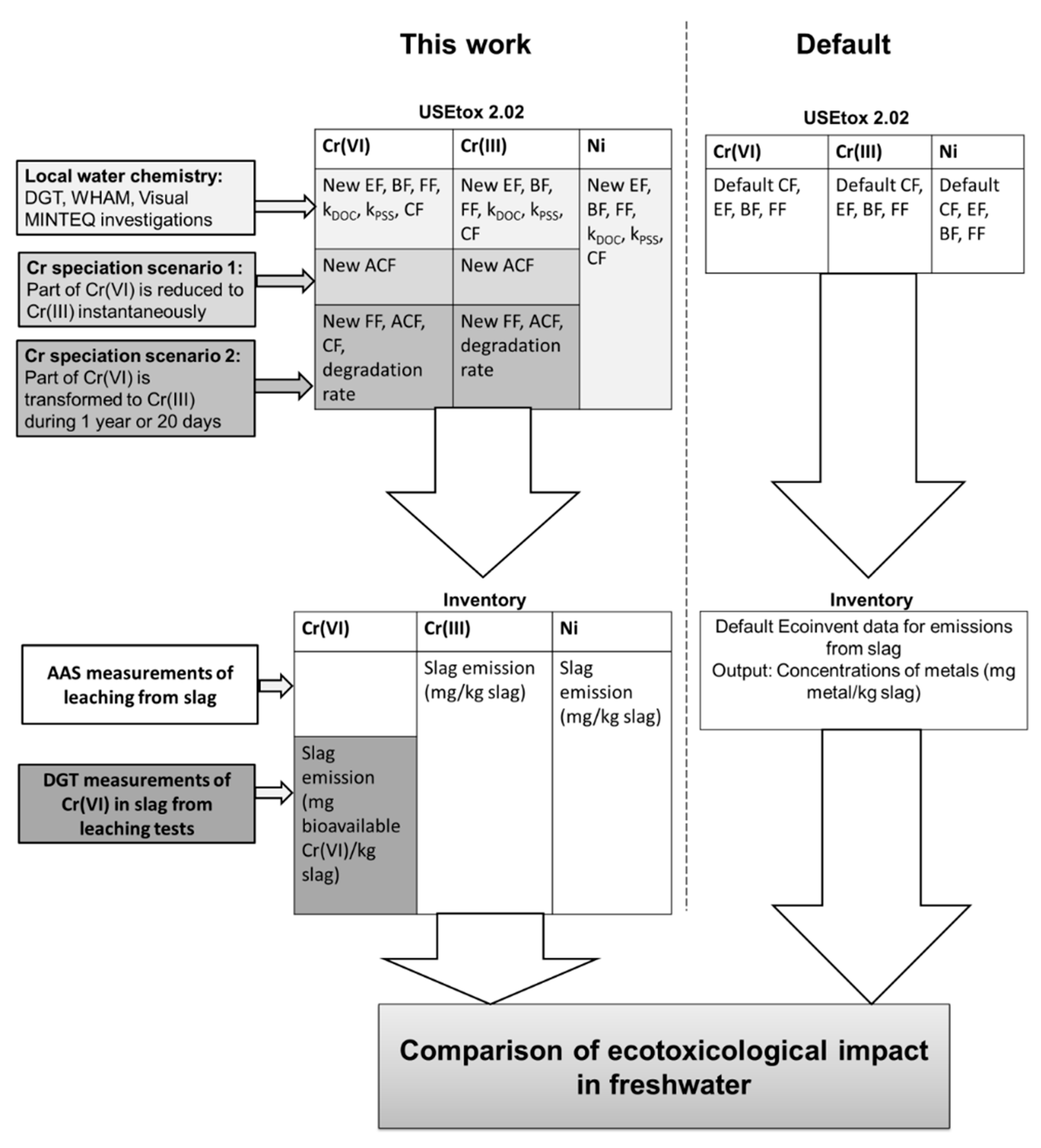
2.1. Construction of Characterization Factors for a Model Freshwater

A model freshwater of relevance for stainless steel production in the Bergslagen region of Sweden was constructed (

Table 1. Basic parameters of the model freshwater based on data collected from the SLU database [24,25].

pH	Dissolved Organic Carbon, DOC (mg/L)	Alkalinity (mg CaCO3/L)	Temperature (°C)	Suspended Particulate Matter (mg/L)
7.3	11	16	11	7.2

SLU—Swedish University of Agricultural Sciences.

; more details in Tables S1 and S2 in Supplementary Information), as none of the alternatives in USEtox or in the EU archetype freshwaters (see Table S3 in Supplementary Information) [14] reflect the water chemistry of the region. This freshwater is representative of the collected slag samples. The suspended particulate matter (SPM) used in the model freshwater were silica-based particles obtained from Sigma Aldrich, Sweden.

USEtox is the consensus impact model available to assess both human and environmental toxicity in LCA [7]. This model includes the physical and chemical properties of chemical substances (including metals) that provide data for CFs calculations. For ecotoxicity, the CF consists of a fate factor (FF), an exposure factor (XF, often also denoted the bioavailability factor, BF) [18], and an effect factor (EF). The FF represents the persistence of a chemical in the environment, the XF/BF represents the bioavailability of a chemical, and the EF represents the change in potentially affected fraction of species due to changes in concentration, see Equation (1):

$$CF=FF·XF·EF$$

(1)

Bioavailability is defined as the metal fraction that readily can be taken up by an aquatic organism and is in this context estimated by the labile fraction [26,27]. Metal complexes that are strongly bonded to organic complexes are generally regarded as non-labile and not bioavailable (specifically adsorbed or covalently bonded).

In this study, the USEtox version 2.02 is applied on the results from the experimental measurements and modeling made for Cr(III), Cr(VI), and Ni. The following input parameters were modified: the partitioning coefficient between suspended solids and water (k_PSS), the partitioning coefficient between dissolved organic carbon and water (k_DOC), and the hazardous concentration (HC50) for the given metal species (see below for details). The partitioning coefficients affect the FF and the HC50 the EF. These parameters and the bioavailable (labile) metal fraction were determined using the DGT technique and predicted using WHAM and Visual MINTEQ as described below.

2.2. Geochemical Modelling of Metal Speciation

Visual MINTEQ was employed to estimate the BF of Cr and Ni in the model freshwater. The composition of the model freshwater was used as input for the calculations (Table 1, Tables S1 and S2) with the pH fixed and the ionic strength calculated by the software. The Stockholm humic model (SHM) was used for modelling metal complexation with humic material [17]. Default parameters were used in these calculations [28], assuming 100% of the dissolved organic matter to consist of fulvic acid and the concentration of dissolved organic matter (DOM) to be 1.65 times higher than the DOC [28]. Surfaces of suspended matter were modelled using ferrihydrite using default parameters.

The Windermere humic acid model, WHAM (ver. 7.05), was used to predicted the bioavailable metal fraction in the model freshwater, and used to model the BF for further use in the LCIA assessment [29]. Particulate matter was modelled as iron oxide. The output data of WHAM was also used to obtain numbers for k_DOC and k_PSS.

2.3. DGT Measurements to Estimate Metal Bioavailability

The bioavailable (labile) fraction of specific metals in freshwater and dispersed from slags was determined using the DGT technique [26,30]. The labile metal fraction is related to metal species that can dissociate relatively fast (mainly free ions and inorganic complexes) and thus readily react with e.g., biological media. This fraction can thus be used as an estimate of the bioavailable fraction of the total amount of released metal [26]. Metals strongly associated with large molecules, e.g., fulvic acids, or strongly attached to particles are hence in general excluded from the labile fraction [26]. DGT has been shown to assess the labile metal fraction in relatively good agreement with equilibrium modelling of freshwater [31].

The DGT is comprised of three layers held together by a plastic casing. The first layer is a membrane filter with a 0.45 µm pore size, the second layer is made up of an ion-permeable gel membrane that only permits diffusion of labile metal species, and the third layer is an ion-exchange resin designed to selectively accumulate metal ions. After exposure of the DGT device to the solution of interest, the resin is removed and the metal of interest is eluted in 1 M HNO₃ during 24 h. More details are given in Section 2.8.

The DGT-accessible concentration is then calculated according to Equation (2) using Fick’s law [27], a constant for metal diffusion, and the volume of the resin, absorbing the metal of interest.

$$C_{DGT}=\frac{C_{sol}\left(V_{HN{O}_3}+V_{gel}\right)b}{f_{e}DtA}$$

(2)

where C_sol is the determined concentration of the specific metal in the eluate (g/L), V_HNO3 is the volume of the eluate (L), V_gel is the volume of the resin gel (L), b is the thickness of the diffusive gel and the membrane (cm), f_e is the elution factor (dimensionless), D is the diffusion coefficient (cm²/s), t is the time (s), and A is the area of the membrane (cm²).

2.4. Construction of New Effects Factors

The same procedure as reported in Dong et al. was followed to construct the BFs and EFs for Ni and Cr(III) for the model freshwater [14,15]. In brief, free ion activity HC50 values were constructed based on the water chemistry of ecotoxicity tests for three different trophic levels (using WHAM). Obtained free ion activity HC50 value were used as input into the WHAM modeling and the resulting truly dissolved fraction, the “truly dissolved HC50” fraction, was used to construct the EF according to EF = 0.5/HC50. The free ion activities used as input into WHAM for calculations of the model freshwater was 1.53·10⁻⁶ M for Ni and 3.17·10⁻¹² M for Cr(III) [14]. The construction of a new EF for Cr(VI) was not possible due to lack of toxicity datasets to calculate the truly dissolved HC50 fraction.

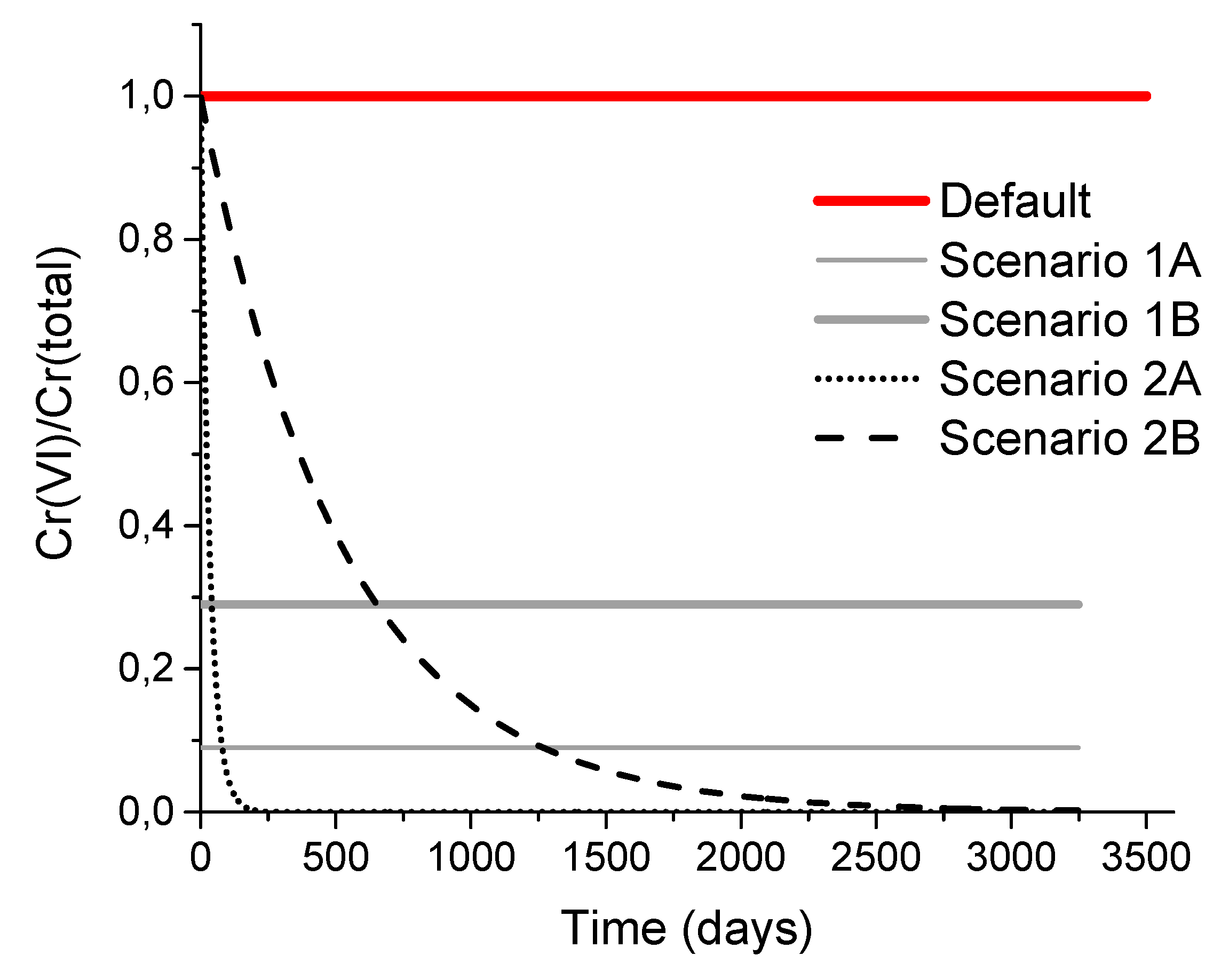
2.5. Scenarios for Taking the Reduction of Cr(VI) into Account in LCIA

The default scenario in the standard USEtox method assumes that an emission of Cr(VI) remains in the same redox state throughout its lifetime and is as such evaluated in LCIA. However, this assumption does for most conditions not necessarily reflect reality as Cr(VI) has a tendency to be reduced at freshwater settings [20]. This is a complex transformation that is not necessarily complete (100%) and that depends on a large number of parameters such as pH, presence and type of natural organic matter (NOM), and presence of Mn- and Fe-oxides [20,32]. Two main scenarios were constructed in order to explore different ways of taking changes in redox state of a Cr(VI) emission into account. These two scenarios are depicted together with the default USEtox treatment of Cr redox (no change of redox state) in Figure 2.

Scenario 1 ignores the kinetics of reduction and assumes that a steady-state level of Cr(VI)/total Cr is obtained instantaneously, which is significantly lower than the initial level. A study of the Cr speciation in Swedish non-urban lakes reports Cr(VI)/Cr(total) ratios varying between 0.44 and 0.77 [33]. This ratio was described by the authors as the soluble fraction of Cr, defined as the fraction filtered through a 0.45 µm pore size membrane. Hence, particulate Cr or Cr attached to particulate matter need to be further considered. Literature data reports the fraction of dissolved Cr to 11% [34] or 20% [35] of the total concentration. As will be shown later this study demonstrates that the partitioning between dissolved Cr(VI) in solution and Cr(VI) bound to particulate matter (ferrihydrite) is 46% in the model freshwater. From this follows the possibility to estimate a lower and an upper boundary for the fraction of Cr(VI) to total(Cr).

The lower boundary (Scenario 1A) was constructed by assuming that 44% of the dissolved Cr is present as Cr(VI) [33] and that these species account for 11% of the total amount of Cr and that the remaining 46% of the Cr(VI) fraction is bound to ferrihydrite. This results in the following calculation to assess the fraction of Cr(VI)/total Cr:

$$\begin{array}{cc}\hfill \frac{Cr\left(VI\right)}{totalCr}\left(min\right)& =\frac{dissolvedCr\left(VI\right)}{totalCr}+\frac{particulateCr\left(VI\right)}{totalCr}\hfill \\ & =0.44\times 0.11+0.44\times 0.11\times \left(\frac{0.46}{0.54}\right)\approx 9\%\hfill \end{array}$$

(3)

Analogously, the upper boundary (Scenario 1B) was estimated by assuming that 77% of the dissolved Cr fraction is present as Cr(VI) and that this phase accounts for 20% of the total amount of Cr, and that the remaining 46% of the Cr(VI) fraction is bound to ferrihydrite. This results in the following calculation for the fraction of Cr(VI)/total Cr:

$$\begin{array}{cc}\hfill \frac{Cr\left(VI\right)}{totalCr}\left(max\right)& =\frac{dissolvedCr\left(VI\right)}{totalCr}+\frac{particulateCr\left(VI\right)}{totalCr}\hfill \\ & =0.77\times 0.20+0.77\times 0.20\times \left(\frac{0.46}{0.54}\right)\approx 29\%\hfill \end{array}$$

(4)

The reduction of Cr(VI) is fast at conditions with high concentrations of reductants (e.g., humic acid, iron oxides) [32]. Scenario 2A represents such a case and assumes a half-life of 20 days for Cr(VI), while scenario 2B assumes a half-life of one year and hence corresponds to a case with low concentrations of reductants in the freshwater [32].

The time-dependent change in the redox state (Scenario 2) was modelled in USEtox by changing the degradation rate of Cr(VI) in freshwater, Equation (5), taking into account the reduction of Cr(VI) to Cr(III):

$$C=C_0{e}^{-k_{deg}·t}$$

(5)

Here, C is the metal species concentration, C₀ is the concentration upon dispersion, t is the time, and k_deg is the degradation constant, which in this case represents the reduction of Cr(VI) to Cr(III). Normally, in USEtox, this degradation rate is set to a very low number for metals (10⁻²⁰ s⁻¹) due to the fact that metals, in contrast to many organic compounds, are not degradable. For a half-life of one year for Cr(VI), this results in a k_deg of 2.2·10⁻⁸ s⁻¹, and for a half-life of 20 days k_deg equals 4.0·10⁻⁷ s⁻¹. The change in degradation rate alters the FF and hence also the CF. The same type of terminology as used in the work by Owsianiak et al. on ageing of metals in soil can be used to describe changes in characterization factors related to changes in Cr(VI) reduction:

$$CF=AC{F}^T·F{F}^T·BF·EF$$

(6)

Here, ACF^T is the accessible fraction of the metal and takes into the account the redox of Cr species, which is time-dependent and represents the metal that is potentially bioavailable [16]. In this work, ACF represents the fraction of the Cr(VI) that has not been reduced to Cr(III):

$$AC{F}^T=\frac{{{\displaystyle \int }}_O^T{f}_{reactive}\left(t\right)dt}{T}$$

(7)

Here, f_reactive(t) is the Cr(VI)/total Cr ratio given in Figure 2 and T is the time horizon for the evaluation. Here, Cr(VI) refers to the total fraction in form of Cr(VI), and the bioavailable fraction is a sub-fraction of this total Cr(VI). Following this definition, the ACF is time-independent for scenario 1 and results in value of 0.09 for scenario 1A and 0.29 for scenario 1B. For scenario 2, the ACF becomes time-dependent, and also the FF as it depends on the degradation rate. Cr(III) formed by the reduction from Cr(VI) will influence the ecotoxicity. This is taken into account by generating a composite CF where the ACF of Cr(III) is simplified to (1-ACF_Cr(VI)). The effect on FF is hence ignored and motivated by the relative short FF for Cr(III) in freshwater [36]. The resulting CF is then calculated as:

$$CF=C{F}_{Cr\left(VI\right)}+C{F}_{Cr\left(III\right)}$$

(8)

2.6. LCIA of Stainless Steel Slags Using SimaPro

In this study, the LCA software SimaPro version 8.5.0.0 was used to model scenarios based on both existing CFs and on constructed CFs. Datasets were generated based on both specific LCI data from experimental metal release tests as well as on data available in the public database Ecoinvent, version 3 (dataset: Slag, unalloyed electric arc furnace steel treatment of, residual material landfill|Alloc Rec, U) [23]. As Cr and Ni were the main metals in focus of this study, only emissions of Cr(III), Cr(VI), and Ni were considered, both for the Ecoinvent dataset and for the generated experimental data.

2.7. Experimental

All vessels and glassware were cleaned with 10% HNO₃ for at least 24 h and rinsed with MilliQ (MQ) water (18 MΩ·cm). The chemicals were used as received, and of reagent grade or higher (>99.0%). The total suspended solids (TSS) for the model freshwater consisted of a 100 mg/L standard purchased from Sigma Aldrich (Sweden). The chemical composition is given in

Table 2. Characteristics of the DGT devices used in this work.

DGT Device	Metals Investigated	Functional Resin	Thickness Resin (cm)	Thickness Diffusive Gel (cm)	Elution Factor	Diffusion Coefficient at 25 °C (m2/s)	Membrane Area (cm2)
LSNM	Cr(III), Ni	Chelex 100 (cross-linked polystyrene matrix with aminodiacetic acid as active group)	0.04	0.074	0.8	5.77·10−6	3.14
LSNE	Cr(VI)	N-methyl-D-glucamine (DMDG)	0.05	0.078	0.712	8.18·10−6	3.14

. Natural organic matter (NOM) for the model freshwater was Nordic Aquatic Fulvic Acid Reference, obtained from the International Humic acid Substance Society (IHSS). The pH of the model freshwater was adjusted using NaOH (reagent grade, >98%) and HNO₃ (suprapur). The addition of metals (Cr, Ni, Al, Fe) to the model freshwater was made using certified atomic absorption standards (Perkin Elmer, 1 g/L) that were further diluted.

2.8. Determination of Total Metal Concentrations in Solution

Atomic absorption spectroscopy (AAS, Perkin Elmer AAnalyst 800) in graphite furnace mode was employed to determine total Ni and Cr concentrations in solution. Calibration standards were prepared from 1 g/L certified metal standards (Perkin Elmer) in 1% HNO₃ solutions. Each sample was measured three times and the resulting average concentration was calculated after subtraction of blank samples (samples without slag or model water without added Cr or Ni). The detection limit was estimated as three times the standard deviation of the blank and the determination limit was calculated as ten times the standard deviation of the same blank. This resulted in detection (LOD) and determination (LOQ) limits of 2.6 and 8.5 µg/L for Ni, and 1.3 and 4.2 µg/L for Cr, respectively.

2.9. Diffusive Gradient in Thin-Films

All experiments were performed as described elsewhere [26,27]. DGT samplers were purchased from DGT Research (Great Britain), consisting of LSNM devices for the determination of Ni and Cr(III) and LSNE devices for measurements of Cr(VI) [37], see Table 1. All devices were stored at 4 °C before usage and conditioned in a 1 mM ionic strength solution prior to the experiments (approximately same ionic strength as the model freshwater).

Model freshwater was freshly prepared before each experiment, see Table 2 for its composition. A volume of 150 mL of model freshwater was used for the DGT experiments, poured into an acid-cleaned polypropylene beaker (250 mL), and covered with parafilm to avoid evaporation. The pH was adjusted using NaOH (reagent grade, >98%) and HNO₃ (suprapur) when necessary to maintain a pH of 7.3. The beakers were exposed at 25 °C on a shaking table at dark conditions in a climatic chamber. The beakers were left to equilibrate for 1 h before the DGT devices were immersed. The devices were taken out from the climatic chamber after 3 days and washed with MQ water. The resin from the DGT samplers was then taken out and eluted in 1 M HNO₃ for 24 h. The total metal concentration of the eluate was analyzed with AAS after appropriate dilution in MQ water. The LOD was approx. 0.13 µg/L and the LOQ was 0.42 µg/L for Cr(VI) for the DGT method.

2.10. Total Metal and Labile Metals of Slag Leachates

Model freshwater, Table 2, was prepared in the same way as for the DGT measurements. Samples with a concentration of 100 mg/L (150 mL freshwater, 15 mg slag particles) were prepared in acid-washed polypropylene beakers (250 mL). The beakers were thoroughly covered with parafilm and placed on a shaking table in dark conditions at 25 °C in a climatic chamber. Aliquots of 6 mL were sampled after 16 days. After completion, the samples were carefully decanted into new acid-cleaned plastic beakers to remove the slag particles. DGT samplers for Cr(VI) detection were placed in each water sample, following the same procedure as described above to quantify the concentration of labile Cr(VI).

2.11. Slag Characterization

Two slag samples were collected from two different stainless steel manufacturing plant in the region of Bergslagen in Sweden. Slag 1 represents an electrical arc furnace manufacturing process and was sampled before any metal recovery. The other slag sample (slag 2) also originated from an electrical arc furnace manufacturing plant (different from slag 1) and was sampled before any metal recovery, but after water cooling of the slag.

Morphological and elemental characteristics of the slags by means of scanning electron microscopy (SEM) and electron dispersion spectroscopy (EDS) are given in Figure S1 and Table S4 (Supplementary Information). SEM and EDS analyses were performed using a Hitachi TM-1000 table-top scanning electron microscope. All images were obtained using backscattered electron mode with an acceleration voltage of 15 keV.

3. Results and Discussion

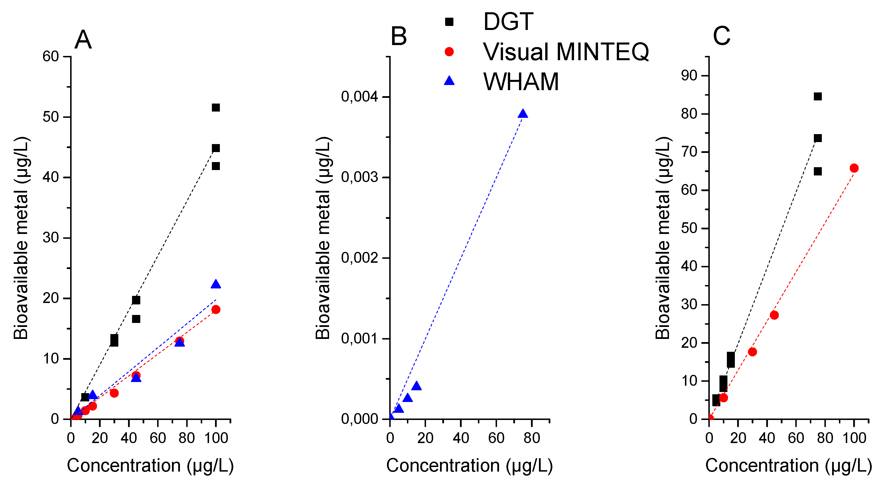
3.1. Comparison between DGT Measurements and Software Simulations for the Construction of Characterization Factors for Cr and Ni in a Model Freshwater

Results of using the different tools to determine/predict metal bioavailability (labile fraction) are exemplified in Figure 3 for Ni, Cr(III), and Cr(VI) in the model freshwater using the DGT technique and the prediction tools WHAM and Visual MINTEQ. Tables S5–S7 compiles the obtained modeling results for each metal using WHAM and Visual MINTEQ, including estimations on whether the complexes can be assigned as labile species or not and hence be regarded as bioavailable.

As seen in Figure 3, all methods were not applicable to all metals. The DGT measurements resulted in concentrations of Cr(III) below the detection limit due to the very low fraction of bioavailable Cr(III), similar to findings using Visual MINTEQ (no reported formation of labile complexes). Cr(VI) modelling is unfortunately not possible in WHAM. The BF (fitted slope in Figure 3) was 0.45 for Ni obtained by DGT, 0.19 for Visual MINTEQ, and 0.20 for WHAM. In the case of Cr(III), the BF was 5·10⁻⁵ as obtained by WHAM. DGT resulted in a BF of 1 for Cr(VI), whereas Visual MINTEQ resulted in a value of 0.64. Observed differences are discussed below.

A large difference in Cr(VI) BF was observed between the DGT measurements and the Visual MINTEQ prediction. This is most probably due to different characteristics of the SPM in the laboratory experiments using silica-based particles for the DGT measurements and iron oxide in the Visual MINTEQ calculations. The modelling results using iron oxide should be a more relevant proxy for SPM. This difference in SPM also affected observed differences between the modelling results and DGT in the case of Ni. These modelling calculations showed no significant adsorption to silica, whereas the binding to iron oxide was ca. 5–12%. The type of SPM can hence have an impact on the BF, and its inclusion models such as USEtox would improve the precision of predictions in freshwater.

The labile metal fraction that DGT probes is not precisely defined. Smaller metal–fulvic acid complexes may diffuse into the DGT device in addition to the diffusion of labile metal species [26]. Since the deployment time of the DGT device of this experiment was relatively long (3 days), it is possible that some metal–FA complexes also are included in the determined fraction of labile complexes measured by DGT and hence overestimated. However, the diffusion of free metal ions is used to estimate the labile fraction (Equation (2)) which normally results in an underestimated value for weak complexes with small organic molecules due to slightly lower diffusion constants in the gel of the DGT compared with free metal ions [26]. Since reported DGT measurements in freshwater show relatively good correlation with modelling of the same systems [26,31], we attribute observed differences in BFs in this study to mainly be a result of the differences in SPM composition. In the following, WHAM data was therefore used to construct the CFs in the model freshwater for Cr(III) and Ni, and Visual MINTEQ for Cr(VI).

The k_DOC and k_PSS partitioning coefficients obtained by WHAM are given in

Table 3. Input parameters for calculation of new characterization factors for Ni, Cr(III), and Cr(VI) in the model freshwater. Default values for USEtox v.2.02 for freshwater are included for comparison.

	kdoc [L/kg]		kpss [L/kg]		HC50 [kg/m3]
	Model Freshwater	Default	Model Freshwater	Default	Model Freshwater	Default
Ni	1.45·105	7.6·104	3.43·104	2.4·103	1.23·10−4	3.61·10−4
Cr(III)	8.77·109	3.8·109	2.76·108	8.9·107	1.64·10−6	4.96·10−7
Cr(VI)	1.00·102	1.00·102	9.58·104	1.6·104	N/A	3.61·10−4

together with new HC50 values that represent literature HC50 values, for which accessibility (the labile fraction) has been taken into account for the model freshwater [14,38] (see Section 2.4). New (corrected) HC50 values were only generated for Ni and Cr(III) due to the lack of data available for Cr(VI). Default USEtox values are included for comparison.

These parameters were used together with BF data presented in the previous section to calculate new FFs and CFs. The results are given in

Table 4. Bioavailability-, fate-, effect- and characterization factors for Ni, Cr(III), and Cr(VI) in the model freshwater. Default numbers from USEtox v.2.02 are included for comparison.

	BF-Bioavailability Factor *		FF-Fate Factor [d]		EF-Effect Factor [PAF·m3·kg−1]		CF-Characterization Factor [PAF·m3·d/kg emitted]
	Model Freshwater	Default	Model Freshwater	Default	Model Freshwater	Default	Model Freshwater	Default
Ni	2.0·10−1	7.1·10−1	6.6·101	1.1·102	4.1·103	3.9·103	9.9·104	3.0·105
Cr(III)	5.0·10−5	7.4·10−4	1.1·101	1.1·101	3.1·105	1.0·106	1.7·102	8.1·104
Cr(VI)	6.4·10−1	8.1·10−1	5.5·101	9.3·101	N/A	1.4·103	4.9·104	1.1·105

* BF is denoted as XF in USEtox 2.02.

along with default values in USEtox v.2.02.

As seen in Table 4, there are some differences between the constructed CFs of the model freshwater and the default values in USEtox. Cr(III) shows the largest difference in CF, in line with large variations of CFs seen for the freshwater archetypes relevant to EU for which the accessibility of metals has been considered in more detail compared with default CFs [14,18]. One reason is the sensitivity of Cr(III) speciation with respect to pH. The large variations between CFs show the importance of designing regional CFs in order to significantly improve the accuracy of the LCIA. Similar findings are reported elsewhere [39]. At present, there are no available CFs for Cr(VI) for the EU freshwater archetypes. The lack of more regional CFs for Cr(VI) further points out the need to, when possible, consider the regional water chemistry.

One improvement for future implementation of CFs for regional freshwaters is to include an option for specifying freshwater water chemistry in USEox (e.g., DOM, pH, alkalinity), and then let the software choose the appropriate CF based on this water chemistry from library of freshwater chemistries.

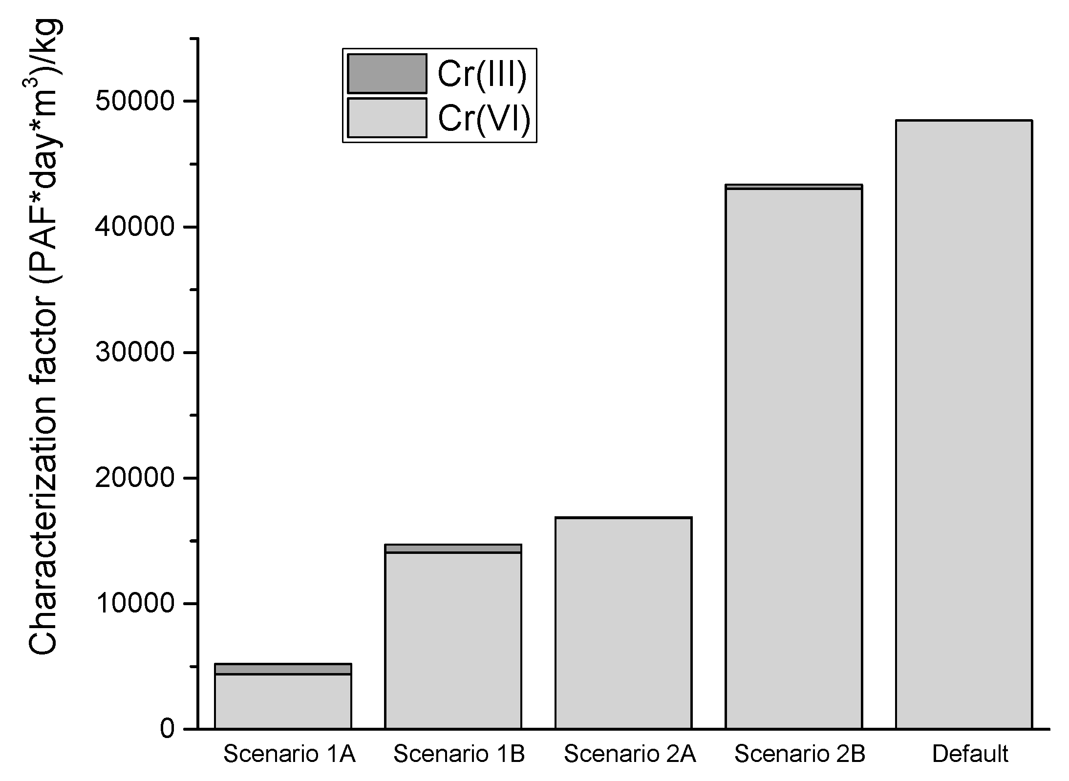
3.2. Comparing Modelling of the Impact of Changes in Cr Oxidation State with the Default Treatment of Cr in USEtox

As described in Section 2.2, two different scenarios were considered to take into account the reduction of Cr(VI) in freshwater. Scenario 1 corresponds to a drop of the Cr(VI)–total Cr ratio that is instantaneous (9% or 29%), and Scenario 2 is a first order degradation of Cr(VI) with a half-life of one year or 20 days. A time horizon has to be selected for the evaluation of the ACF and FF for scenario 2, as shown in Equations (3) and (4). Here we chose time horizons corresponding to the time spans of the calculated FFs in order to take into account the sedimentation and relatively short residence time of Cr(VI) in the freshwater compartment. The results are compiled in

Table 5. Factors for calculation of CFs for the different scenarios of treating Cr(VI) reduction in freshwater.

	Degradation Rate [s−1]	Fate Factor [d]	Accessibility Factor	Characterization Factor, Cr(VI) [PAF·m3·d/kg emitted]	Characterization Factor, Cr(III) [PAF·m3·d/kg emitted]	Characterization Factor, Total [PAF·m3·d/kg emitted]
Scenario 1A	1·10−20	5.5·101	0.09	3.4·103	8.4·102	5.2·103
Scenario 1B	1·10−20	5.5·101	0.29	1.4·104	6.5·102	1.5·104
Scenario 2A	2.2·10−8	5.2·101	0.93	4.3·103	6.5·101	4.3·104
Scenario 2B	4.0·10−7	3.0·101	0.63	1.7·107	3.4·102	1.7·104

, including the contribution of Cr(III) (CF, Cr(III)) as a result of Cr(VI) reduction by using Equation (8). The resulting CFs for the scenarios and the default CF in USEtox are presented in Figure 4.

Observed differences between the scenarios in Figure 4 lie within the uncertainty stated in USEtox for the CFs of ecotoxicity (100–1000 times) [7]. The introduction of Cr speciation in LCIA nonetheless rectifies an otherwise inherent overestimation of metal toxicity in the default USEtox assessment due to the static Cr(VI) speciation in case of dispersion of such species.

One option for implementing changes in Cr(VI) speciation in USEtox is to include a Cr(VI)–Cr(total) ratio based on literature findings for a given freshwater chemistry, just as in Scenario 1, which can be used to calculate a ACF This is in the vein of the USEtox strategy to provide general data and trends for evaluating the environmental impact. A starting point for Cr speciation in USEtox should be experimental data, as modelling of Cr speciation is of such complexity that it requires more work before any robust models will be available [40]. The DGT method could come to use here and investigate the labile Cr(VI) fraction as a function of time. The reduction of Cr(VI) could also be added to the assessment of the soil compartment using a similar approach conducted by Owsiniak et al. [39], and the construction of time-dependent ACFs and FFs.

In the meantime, before any implementation of redox changes in USEtox, LCA users should be aware of that toxicity in LCIA resulting from the dispersion of Cr(VI) to freshwater is overestimated. This is especially important when the relative contribution of such a dispersion dominates in the impact assessment.

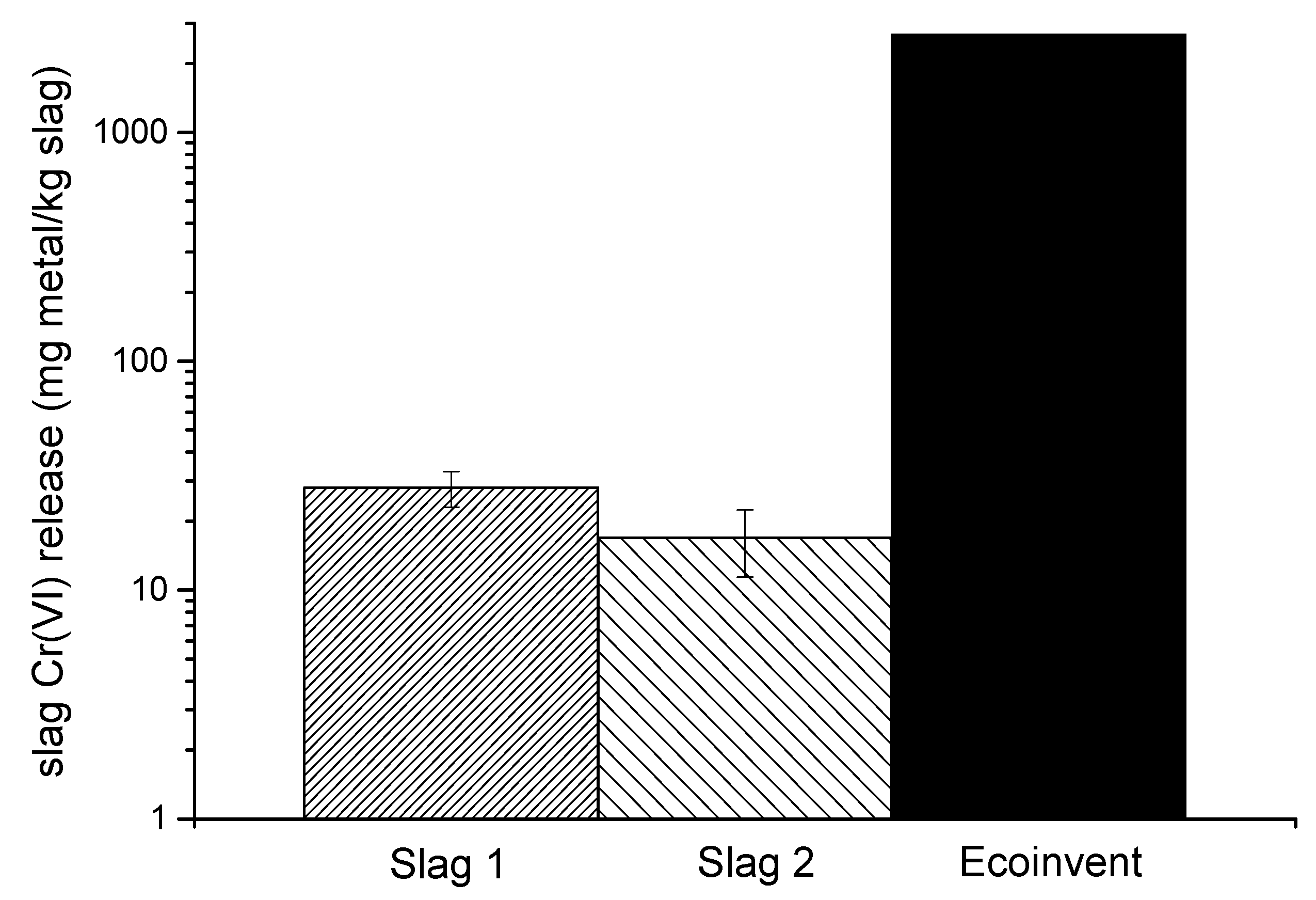
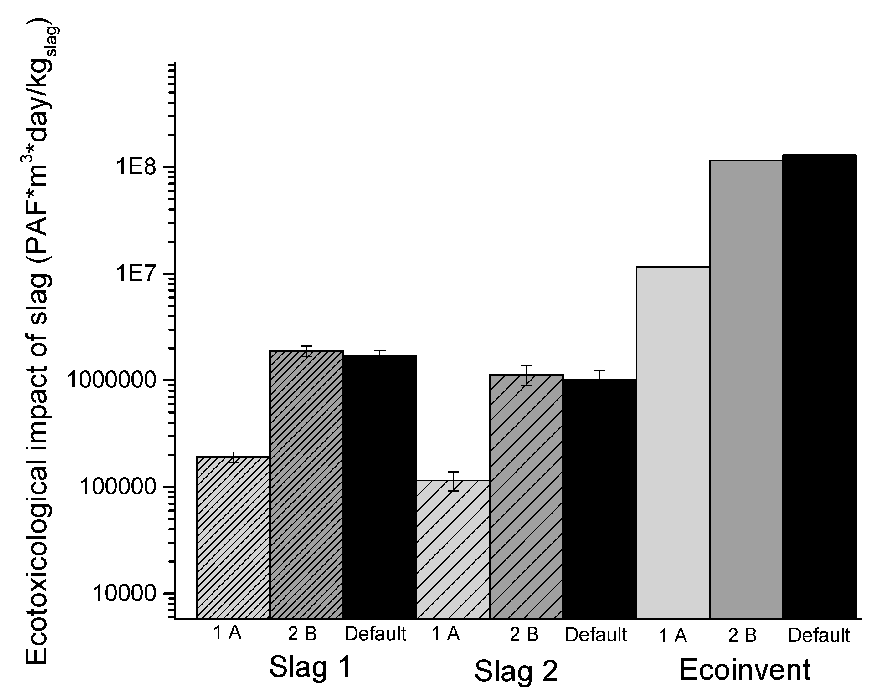
3.3. Implementing Experimental Data in LCIA on Metal Bioavailability of Cr(VI), Cr(III), and Ni Dispersed from Slag and Comparisons between the Use of Data and Default Values in USEtox

In this section, metal release (leaching) results from the collected slags will be compared with default Ecoinvent data for metal emissions from slags, applying the CFs generated in this study on the model freshwater and the scenarios for Cr(VI) reduction.

The DGT results for Cr(VI) released from two different slags are presented in Figure 5 (see Supplementary Information for additional slag characteristics). These slags represent worst case scenarios in the sense that they are sampled before any metal recovery, which means a higher metal content than typically for slags in landfills, and lack of time for ageing that in general results in a less reactive slag (less soluble metal oxides/minerals) over time [11,16].

The emission of Cr(VI) to freshwater is the largest emission in the current Ecoinvent data set with minor emissions taking place to river water, soil, and air. The Ecoinvent data for emissions to groundwater was used to model emissions to freshwater as no CFs in USEtox exist for emissions to groundwater. The amount shown in Figure 5 hence corresponds to the sum of emissions to both river and groundwater. Total release data of Cr and Ni from the slags were determined (not DGT) and measured by AAS. These results showed released concentrations being close to, or below the detection limit (see Section 2.8). For Cr, this implies that most of the released Cr was present as Cr(VI) as the detection limit is close to the observed concentration of Cr(VI) by means of DGT. The release of Cr as Cr(VI) from slags is expected to be larger than the amount of Cr(III) species released due to the formation of insoluble minerals and Cr(OH)₄⁻ [40], which make the released Cr(III) concentrations very low. Observed levels of released Cr(VI) were in the same order of magnitude as observed in the literature [41]. These results further imply that no Cr(VI) was reduced over the time frame of the DGT experiments (16 days) and shows that the model freshwater composition does not favor fast reduction kinetics (Scenario 2A).

Variations in the slag inventory data (Figure 5) can be larger than dissimilarities in CFs obtained by including different scenarios for the reduction of Cr(VI) (Figure 4). The variations in available slag release data hence have a high potential to overshadow the Cr(VI) reduction effects even though it is evident that information on the Cr(VI) reduction kinetics certainly improves the relevance of the LCIA.

It is important to point out that the DGT results are not directly comparable with literature findings and default Ecoinvent data from metal leaching from slags, as the DGT technique assesses the labile fraction of metals, as described previously. A BF has to be applied to measurements of total metal concentrations in order to make them somewhat comparable.

Figure 6 shows the slag release data multiplied by the appropriate CFs (depicted in Figure 4) without any BF involved in the calculations for the slag release measured using DGT. The CFs values are given in Table 5 and represent the total CF (both Cr(VI) and Cr(III) contributions). Calculations for the different scenarios 1A and 2B, i.e., freshwaters with fast reduction kinetics (1A) and slow reduction kinetics (2B), result in an approximately one order of magnitude difference in ecotoxicological impact.

A total difference of 2–3 orders of magnitude between introducing the different Cr(VI) scenarios and the default setting (Ecoinvent data with default CFs) is evident from the results of Figure 6. This underlines the importance of having and using relevant inventory data for slags in LCIA. The outlined methodology and strategy as presented in this study (Figure 2) can hence be useful for anyone doing an in-depth characterization of the ecotoxic impact in LCIA induced by the dispersion of metals from slag or any other source of metal dispersion.

The importance of slag release (or any release of metals from a landfill) in the context of LCIA has been recognized previously [12,16]. Most metals in slags are though recovered via different processes such as magnetic separation [42,43]. If not used in different applications, the slag, air-cooled or treated, is stored in landfills. Consequently, the slag predominantly contains (>80%) silica, calcium carbonate, aluminum oxide, manganese oxide, and calcium hydroxide and only to a minor part metals such as Ni and Cr [42]. Most of the metal content in the slag remains even after 100 years in a landfill (>ca. 99%) due to their presence as low solubility compounds/minerals [11]. If dispersed into an aqueous setting, released metals from the slag will to some extent be further transformed into even less soluble oxides [16]. Owsiniak et al. introduced, as mentioned, the ACF to take into account ageing of metals in soil in order to capture the trend of lower reactivity of metals as they form more and more stable oxides over time [39]. This study does not give any new insights into treatment of long-term emissions from slags, but it can be noted that the relatively short residence time of Cr(VI) in freshwater (55 days or shorter in this study) implies that, as seen earlier [36], this compartment will not be severely affected by long term ageing of the metals. DGT can be a useful tool to estimate both the bioavailable (labile) fraction of metals and to provide information on leaching kinetics in soils and sediments for long-term experiments [44]. The technique can also provide information on chemical speciation, such as Cr(VI) as shown in this study. A suggestion in this regard is to combine results of metal release investigations in terms of standard batch testing with metal release testing of minerals (relevant metal oxides that are known and expected to form and exist also after hundreds and thousands of years).

Another way forward could be that future inventory data in the Ecoinvent database for slags becomes more detailed, including metal release test procedures as well as slag characteristics (e.g., total metal content), as suggested previously [16]. Such data could help in modelling of metal release [45], and provide additional information on what the inventory data means in terms of time frames for the emissions being modelled. Another uncertainty lies in the lack of CFs for emissions to groundwater [46].

4. Conclusions

This study outlies a strategy to improve LCIA of metal release from slags in terms of ecotoxicity. CFs relevant for stainless steel manufacturing regions in Sweden were constructed by speciation measurements and predictions of Cr and Ni using DGT, Visual MINTEQ, and WHAM in model freshwater. Cr speciation should be considered in LCIA due to its documented changes in the redox state of Cr(VI) emissions to freshwater. The introduction of different realistic scenarios for changes in Cr(VI) levels with time resulted in up to one order of magnitude lower ecotoxic impact compared with the standard option in LCIA (no redox state change). A proposal on how to implement Cr speciation in LCIA to counteract the current overestimation of metal toxicity in the default USEtox assessment is to include a general steady-state relationship between Cr(VI)/Cr(total). The DGT method was used to assess the release of Cr(VI) from slags sampled from two stainless steel production sites. All in all, the most significant relative influence on the ecotoxicological impact was observed for metal release from slag, as the different options on how to assess and model metal emissions from slags spanned more than two orders of magnitude, in addition to the one order of magnitude span observed for different CFs. In the future, it should be prioritized to account for changes in Cr speciation in LCIA and that the assessment is made for freshwater conditions of relevance for the region of interest, e.g., at aquatic settings adjacent a stainless steel manufacturing plant.

References

1. Norgate, T.; Jahanshahi, S.; Rankin, W. Assessing the environmental impact of metal production processes. J. Clean. Prod. 2007, 15, 838–848. [Google Scholar] [CrossRef]
2. Finkbeiner, M.; Inaba, A.; Tan, R.; Christiansen, K.; Klüppel, H.-J. The new international standards for life cycle assessment: ISO 14040 and ISO 14044. Int. J. Life Cycle Asses. 2006, 11, 80–85. [Google Scholar] [CrossRef]
3. Guinée, J. Handbook on life cycle assessment—Operational guide to the ISO standards. Int. J. Life Cycle Asses. 2001, 6, 255. [Google Scholar] [CrossRef]
4. EC—European Commission. International Reference Life Cycle Data System (ILCD) Handbook—General Guide for Life Cycle Assessment—Detailed Guidance; Joint Research Centre Institute for Environment and Sustainability: Ispra (VA), Italy, 2010. [Google Scholar]
5. ISO—International Organization for Standardization. Environmental Management—Life Cycle Assessment -Principals and Framework; International Standard ISO 14040; ISO: Geneva, Switzerland, 2006. [Google Scholar]
6. ISO—International Organization for Standardization. Environmental Management—Life Cycle Assessment—Requirements and Guidelines; International Standard ISO 14044; ISO: Geneva, Switzerland, 2006. [Google Scholar]
7. Rosenbaum, R.K.; Bachmann, T.M.; Gold, L.S.; Huijbregts, M.A.; Jolliet, O.; Juraske, R.; Koehler, A.; Larsen, H.F.; MacLeod, M.; Margni, M. USEtox—the UNEP-SETAC toxicity model: Recommended characterisation factors for human toxicity and freshwater ecotoxicity in life cycle impact assessment. Int. J. Life Cycle Assess. 2008, 13, 532–546. [Google Scholar] [CrossRef]
8. Fantke, P.; Aurisano, N.; Bare, J.; Backhaus, T.; Bulle, C.; Chapman, P.M.; De Zwart, D.; Dwyer, R.; Ernstoff, A.; Golsteijn, L. Toward Harmonizing Ecotoxicity Characterization in Life Cycle Impact Assessment. Environ. Toxicol. Chem. 2018, 37, 2955–2971. [Google Scholar] [CrossRef] [PubMed]
9. Saouter, E.; Aschberger, K.; Fantke, P.; Hauschild, M.Z.; Kienzler, A.; Paini, A.; Pant, R.; Radovnikovic, A.; Secchi, M.; Sala, S. Improving substance information in USEtox®, part 2: Data for estimating fate and ecosystem exposure factors. Environ. Toxicol. Chem. 2017, 36, 3463–3470. [Google Scholar] [CrossRef]
10. Baumann, H.; Tillman, A. The Hitchhiker’s Guide to LCA, an Orientation in Life Cycle Assessment Methodology and Application; Studentlitteratur: Lund, Sweden, 2004. [Google Scholar]
11. Hauschild, M.; Olsen, S.I.; Hansen, E.; Schmidt, A. Gone… but not away—Addressing the problem of long-term impacts from landfills in LCA. Int. J. Life Cycle Assess. 2008, 13, 547. [Google Scholar] [CrossRef]
12. Bakas, I.; Hauschild, M.Z.; Astrup, T.F.; Rosenbaum, R.K. Preparing the ground for an operational handling of long-term emissions in LCA. Int. J. Life Cycle Assess. 2015, 20, 1444–1455. [Google Scholar] [CrossRef] [Green Version]
13. Hauschild, M.Z.; Huijbregts, M.; Jolliet, O.; Macleod, M.; Margni, M.; van de Meent, D.; Rosenbaum, R.K.; McKone, T.E. Building a model based on scientific consensus for life cycle impact assessment of chemicals: The search for harmony and parsimony. Environ. Sci. Technol. 2008, 42, 7032–7037. [Google Scholar] [CrossRef]
14. Dong, Y.; Gandhi, N.; Hauschild, M.Z. Development of Comparative Toxicity Potentials of 14 cationic metals in freshwater. Chemosphere 2014, 112, 26–33. [Google Scholar] [CrossRef] [PubMed]
15. Dong, Y.; Rosenbaum, R.K.; Hauschild, M.Z. Assessment of metal toxicity in marine ecosystems: Comparative toxicity potentials for nine cationic metals in coastal seawater. Environ. Sci. Technol. 2015, 50, 269–278. [Google Scholar] [CrossRef] [PubMed]
16. Owsianiak, M.; Holm, P.E.; Fantke, P.; Christiansen, K.S.; Borggaard, O.K.; Hauschild, M.Z. Assessing comparative terrestrial ecotoxicity of Cd, Co, Cu, Ni, Pb, and Zn: The influence of aging and emission source. Environ. Pollut. 2015, 206, 400–410. [Google Scholar] [CrossRef] [PubMed] [Green Version]
17. Gustafsson, J. Visual MINTEQ ver. 3.0; KTH Department of Land and Water Resources Engineering: Stockholm, Sweden, 2011; (Based on de Allison JD, Brown DS, Novo-Gradac KJ, MINTEQA2 ver. 4, 1991). [Google Scholar]
18. Gandhi, N.; Diamond, M.L.; van de Meent, D.; Huijbregts, M.A.; Peijnenburg, W.J.; Guinée, J. New method for calculating comparative toxicity potential of cationic metals in freshwater: Application to copper, nickel, and zinc. Environ. Sci. Technol. 2010, 44, 5195–5201. [Google Scholar] [CrossRef]
19. Chattopadhyay, B.; Utpal, S.; Mukhopadhyay, S. Mobility and bioavailability of chromium in the environment: Physico-chemical and microbial oxidation of Cr (III) to Cr (VI). J. Appl. Sci. Environ. Manag. 2010, 14, 97–101. [Google Scholar] [CrossRef]
20. Richard, F.C.; Bourg, A.C. Aqueous geochemistry of chromium: A review. Water Res. 1991, 25, 807–816. [Google Scholar] [CrossRef]
21. Schwab, O.; Bayer, P.; Juraske, R.; Verones, F.; Hellweg, S. Beyond the material grave: Life Cycle Impact Assessment of leaching from secondary materials in road and earth constructions. Waste Manag. 2014, 34, 1884–1896. [Google Scholar] [CrossRef]
22. Allegrini, E.; Butera, S.; Kosson, D.; Van Zomeren, A.; Van der Sloot, H.; Astrup, T.F. Life cycle assessment and residue leaching: The importance of parameter, scenario and leaching data selection. Waste Manag. 2015, 38, 474–485. [Google Scholar] [CrossRef]
23. Wernet, G.; Bauer, C.; Steubing, B.; Reinhard, J.; Moreno-Ruiz, E.; Weidema, B. The ecoinvent database version 3 (part I): Overview and methodology. Int. J. Life Cycle Asses. 2016, 21, 1218–1230. [Google Scholar] [CrossRef]
24. SLU—Institutionen för Vatten och Miljö. Ö Storsjön, 1,2 km V Stensängsholmen. Available online: http://info1.ma.slu.se/max/www_max.acgi$Station?ID=Intro&pID=38&sID=2219 (accessed on 3 March 2017).
25. SLU—Institutionen för Vatten och Miljö. V Storsjön. 1,2 km O Gravholmen. Available online: http://info1.ma.slu.se/max/www_max.acgi$Station?ID=Intro&pID=38&sID=2218 (accessed on 3 March 2017).
26. Zhang, H.; Davison, W. Use of diffusive gradients in thin-films for studies of chemical speciation and bioavailability. Environ. Chem. 2015, 12, 85–101. [Google Scholar] [CrossRef]
27. Davison, W.; Zhang, H. Progress in understanding the use of diffusive gradients in thin films (DGT)–back to basics. Environ. Chem. 2012, 9, 1–13. [Google Scholar] [CrossRef]
28. Sjöstedt, C.S.; Gustafsson, J.P.; Köhler, S.J. Chemical equilibrium modeling of organic acids, pH, aluminum, and iron in Swedish surface waters. Environ. Sci. Technol. 2010, 44, 8587–8593. [Google Scholar] [CrossRef] [PubMed]
29. Tipping, E. WHAMC—A chemical equilibrium model and computer code for waters, sediments, and soils incorporating a discrete site/electrostatic model of ion-binding by humic substances. Comput. Geosci. 1994, 20, 973–1023. [Google Scholar] [CrossRef]
30. Zhang, H.; Davison, W. Performance characteristics of diffusion gradients in thin films for the in situ measurement of trace metals in aqueous solution. Anal. Chem. 1995, 67, 3391–3400. [Google Scholar] [CrossRef]
31. Unsworth, E.R.; Warnken, K.W.; Zhang, H.; Davison, W.; Black, F.; Buffle, J.; Cao, J.; Cleven, R.; Galceran, J.; Gunkel, P.; et al. Model Predictions of Metal Speciation in Freshwaters Compared to Measurements by In Situ Techniques. Environ. Sci. Technol. 2006, 40, 1942–1949. [Google Scholar] [CrossRef] [PubMed] [Green Version]
32. Munn, S.; Allanou, R.; Aschberger, K.; Berthault, F.; Cosgrove, O.; Luotamo, M.; Pakalin, S.; Paya-Perez, A.; Pellegrini, G.; Schwarz-Schulz, B. Chromium trioxide, sodium chromate, sodium dichromate, ammonium dichromate, potassium dichromate, EUR 21508 EN. Eur. Union Risk Assess. Rep. 2005, 53. [Google Scholar]
33. Woldegiorgis, A. Results from the Swedish Screening Programme 2006. Subreport 5: Hexavalent Chromium, Cr (IV). IVL Swedish Environmental Research Institute; IVL Swedish Environmental Research Institute: Stockholm, Sweden, 2007. [Google Scholar]
34. Crommentuijn, T.; Sijm, D.; De Bruijn, J.; Van den Hoop, M.; Van Leeuwen, K.; Van de Plassche, E. Maximum permissible and negligible concentrations for metals and metalloids in the Netherlands, taking into account background concentrations. J. Environ. Manag. 2000, 60, 121–143. [Google Scholar] [CrossRef]
35. Ableitung und Erprobung von Zielvorgaben zum Schutz Oberirdischer Binnengewässer für die Schwermetalle Blei, Cadmium, Chrom, Kupfer, Nickel, Quecksilber und Zink. (Derivation and Proof Testing of Target Settings for the Protection of the Aboveground Inland Waters for the Heavy Metals Lead, Cadmium, Chrome, Copper, Mercury and Zinc.); Kulturbuchverlag: Berlin, Germany, 1994; ISBN 3-88961-216-4.
36. Garnier, J.-M.; Ciffroy, P.; Benyahya, L. Implications of short and long term (30 days) sorption on the desorption kinetic of trace metals (Cd, Zn, Co, Mn, Fe, Ag, Cs) associated with river suspended matter. Sci. Total Environ. 2006, 366, 350–360. [Google Scholar] [CrossRef] [PubMed]
37. Pan, Y.; Guan, D.-X.; Zhao, D.; Luo, J.; Zhang, H.; Davison, W.; Ma, L.Q. Novel speciation method based on diffusive gradients in thin-films for in situ measurement of CrVI in aquatic systems. Environ. Sci. Technol. 2015, 49, 14267–14273. [Google Scholar] [CrossRef]
38. Gandhi, N.; Diamond, M.; Huijbregts, M.J.; Guinée, J.; Peijnenburg, W.G.M.; Meent, D. Implications of considering metal bioavailability in estimates of freshwater ecotoxicity: Examination of two case studies. Int. J. Life Cycle Assess. 2011, 16, 774–787. [Google Scholar] [CrossRef]
39. Owsianiak, M.; Rosenbaum, R.K.; Huijbregts, M.A.; Hauschild, M.Z. Addressing geographic variability in the comparative toxicity potential of copper and nickel in soils. Environ. Sci. Technol. 2013, 47, 3241–3250. [Google Scholar] [CrossRef]
40. Cornelis, G.; Johnson, C.A.; Van Gerven, T.; Vandecasteele, C. Leaching mechanisms of oxyanionic metalloid and metal species in alkaline solid wastes: A review. Appl. Geochem. 2008, 23, 955–976. [Google Scholar] [CrossRef]
41. Loncnar, M.; Zupan, M.; Bukovec, P.; Jakli, A. The effect of water cooling on the leaching behaviour of EAF slag from stainless steel production. Mater. Technol. Mater. Technol. 2009, 43, 315–321. [Google Scholar]
42. Shen, H.; Forssberg, E.; Nordström, U. Physicochemical and mineralogical properties of stainless steel slags oriented to metal recovery. Resour. Conserv. Recy. 2004, 40, 245–271. [Google Scholar] [CrossRef]
43. Lopez, F.; Lopez-Delgado, A.; Balcazar, N. Physico-Chemical and Mineralogical Properties of EAF and AOD Slags; Associazione Italiana di Metallurgia: Milano, Italy, 1997; pp. 417–426. [Google Scholar]
44. Schmukat, A.; Duester, L.; Ecker, D.; Heininger, P.; Ternes, T. Determination of the long-term release of metal (loid) s from construction materials using DGTs. J. Hazard. Mater. 2013, 260, 725–732. [Google Scholar] [CrossRef]
45. Astrup, T.; Mosbæk, H.; Christensen, T.H. Assessment of long-term leaching from waste incineration air-pollution-control residues. Waste Manag. 2006, 26, 803–814. [Google Scholar] [CrossRef] [PubMed]
46. Turner, D.A.; Beaven, R.P.; Woodman, N.D. Evaluating landfill aftercare strategies: A life cycle assessment approach. Waste Manag. 2017, 63, 417–431. [Google Scholar] [CrossRef] [PubMed] [Green Version]
Figure 1. Outline of the strategy of this study including construction of new fate factors (FF), effect factors (EF), bioavailability factors (BF), accessibility factors (ACF), and characterization factors (CFs). New partitioning coefficients were determined between metals in solution and dissolved organic matter, as well as for suspended solids (PSS) (kDOC, kPSS). The degradation rate was changed in order to take into account the reduction of Cr(VI) to Cr(III). The diffuse gradient in thin-film technique (DGT) was used to estimate bioavailable (labile metals—free ions and easily soluble metal complexes) metals in solution, and atomic absorption spectroscopy (AAS) to determine total concentrations of metals in solution (independent on metal speciation).
Sustainability 11 01655 g001
Figure 2. Description of scenarios for treatment of Cr(VI) reduction in USEtox. Default is the standard way in USEtox (no change in Cr(VI) speciation), Scenario 1 is an instantaneous reduction of the Cr(VI)/Cr ratio, and Scenario 2 is a first-order reduction of Cr(VI) with a half-life of 20 days (2A) and one year (2B).
Sustainability 11 01655 g002
Figure 3. Investigation of the bioavailable (labile) concentration of (A) Ni, (B) Cr(III), and (C) Cr(VI) in the model freshwater. Multiple data points represent individual samples for the DGT investigations. The dotted lines are linear fits to the respective dataset.
Sustainability 11 01655 g003
Figure 4. The contribution of Cr(III) and Cr(VI) to the total CF for the different scenarios that take into account Cr(VI) reduction, compared with the default approach in USEtox that does not consider this process.
Sustainability 11 01655 g004
Figure 5. Release of Cr(VI) from slags sampled prior to metal recovery (worst-case scenarios). Data for slags 1 and 2 was generated based on DGT measurements in this study. The Ecoinvent result corresponds to available data in its database for stainless steel slag (sum of emissions to river and groundwater).
Sustainability 11 01655 g005
Figure 6. Ecotoxicological impact of Cr(VI) released from slag (Slag 1 and 2) and Cr(VI) release assessed from Ecoinvent data for slags relevant for stainless steel manufacturing. The CFs from scenarios 1A and 2B were used together with default CFs in USEtox for freshwater.
Sustainability 11 01655 g006