Financial Stability and Sustainability under the Coordination of Monetary Policy and Macroprudential Policy: New Evidence from China


1
School of Economics, Sichuan University, Chengdu 610065, China
2
The Fuqua School of Business, Duke University, Durham, NC 27708, USA
3
Department of Transportation, Logistics and Finance, North Dakota State University, Fargo, ND 58108, USA
*
Authors to whom correspondence should be addressed.
Sustainability 2019, 11(6), 1616; https://doi.org/10.3390/su11061616
Submission received: 15 February 2019
/
Revised: 11 March 2019
/
Accepted: 13 March 2019
/
Published: 18 March 2019
(This article belongs to the Section Economic and Business Aspects of Sustainability)
Abstract
:After the financial crisis, financial stability and sustainability became key to global economic and social development, and the coordination of monetary policy and macroprudential policy plays a crucial role in maintaining financial stability and sustainability. This paper provides a theoretical analysis and empirical evidence from China on the impact of monetary policy and macroprudential policy coordination on financial stability and sustainability. We collect data from 2003 to 2017; from the micro level, we use the System Generalized Method of Moments (System GMM) method to analyze the monetary policy and macroprudential policy coordination effect on 88 commercial banks’ risk-taking; from the macro level, we use the Structural Vector Autoregression (SVAR) method to analyze the two policies coordination effect on housing prices and stock price bubbles. The conclusions are as follows: firstly, for regulating bank risk-taking, monetary policy and macroprudential policy should conduct counter-cyclical regulation simultaneously; secondly, for regulating housing prices, tight monetary policy and tight macroprudential policy should be implemented alternately; thirdly, for regulating stock price bubbles, macroprudential policy should be the first line of defense and monetary policy should be the second one.
1. Introduction
After the 2008 financial crisis, financial stability and sustainability have become the key to global economic development, and monetary policy only focusing on price stability has proved inadequate for maintaining financial stability and sustainability. In this context, macroprudential policy aimed at preventing systemic risk by restraining the excessive risk-taking of financial market participants beforehand becomes another important guarantee for financial stability and sustainability in the post-crisis era. Because monetary policy and macroprudential policy have some overlapping transmission channels to the economy, the coordination of two policies is vital.
This study analyzes the impact of the coordination of China’s monetary policy and macroprudential policy on important financial stability and sustainability indicators: bank risk-taking and asset prices from the micro and macro levels. From the micro level, we use the System Generalized Method of Moments (System GMM) method to analyze the monetary policy and macroprudential policy coordination effect on the risk-taking of 88 of China’s commercial banks; from the macro level, we use the Structural Vector Autoregression (SVAR) method to analyze the two policies coordination effect on China’s housing prices and stock prices. The aim is to conclude the coordination effect of monetary policy and macroprudential policy in China and to provide some inspiration on financial stability and sustainability around the world.
The remainder of this paper is organized as follows. In Section 2, we provide a comprehensive literature review on financial stability and sustainability, macroprudential policy, and the coordination of monetary policy and macroprudential policy. In Section 3, we layout a theoretical analysis and research hypotheses on the effect of monetary and macroprudential policy on bank risk-taking and housing and stock prices. In Section 4, the empirical analysis and robustness check are presented, and finally the conclusion is given in Section 5.
2. Literature Review
Before the crisis of 2008, the global economy enjoyed 20 years of steady and rapid growth, often called the Great Moderation. During that period, financial stability and sustainability were neglected. But with the outbreak of the financial crisis, financial stability and sustainability have once again come to the fore. So far, there is no accepted definition of financial stability, some scholars use characteristics of financial stability to describe its connotation directly [1,2,3], while some define financial stability from the opposite side, namely financial instability [4,5,6]. In general, financial stability should meet the following characteristics: first, stable currency value and function; second, major financial institutions and financial markets operate normally and allocate resources efficiently; third, asset prices wo not change dramatically; fourth, the financial system can withstand shocks to prevent adverse impacts on the real economy. Financial sustainability is based on the premise of following the objective law of financial development, the financial industry can reasonably and effectively allocate financial resources to maintain the development and stability of finance and real economy in the long run. Although financial stability and sustainability are two concepts, there is a close interaction between them. Firstly, financial stability is a necessary prerequisite for sustainability. Only with financial stability can the financial system give full reign to its role in the inter-temporal allocation of resources and promote the sustainable development of the finance and the economy. Secondly, financial sustainability is an essential basis for financial stability. The increasing efficiency of financial services, the increasing ability to integrate financial services with the real economy, and the increasing resilience of financial markets have all effectively contributed to financial stability. Therefore, this paper takes financial stability and sustainability as a whole and takes them together as the goal of monetary policy and macroprudential policy coordination.
During the Great Moderation, the traditional monetary policy aimed at price stability was once thought to be perfect and it has some main characteristics, such as focusing only on the single goal of inflation [7], not taking asset prices and financial stability into account, and remedying after the bursting of asset price bubbles [8]. The traditional financial supervision policy with micro-prudential supervision at the core believes that the safety and stability of individual financial institutions can ensure the overall safety and stability of the financial system [9]. However, the pro-cyclical nature of finance and systemic risk exposed by the financial crisis has shown that the macro financial management framework formed by monetary policy controlling for inflation and micro-prudential supervision has many defects [10,11]. In the post-crisis era, a term often associated with financial stability and sustainability is “macroprudential”. Macroprudential is not a term that emerged only after the 2008 financial crisis [12]. Back in the 1970s, the Cook Committee, the predecessor of the Bank for International Settlements, first adopted the word “macroprudential” in a document and proposed that financial regulation should have a systematic macro perspective. In 2011, the International Monetary Fund, the Bank for International Settlements, and the Financial Stability Board jointly defined macroprudential policy clearly as policies using prudential policies as tools, supported by the necessary governance structures aimed at preventing the systemic risk [13]. At present, the research on macroprudential policy mainly focuses on the policy subject, the policy tools, the policy effectiveness, and the coordination between monetary policy and macroprudential policy. Among them, the coordination between monetary policy and macroprudential policy is the frontier issue of the field and also the core issue of this paper.
The reason why monetary policy should coordinate with macroprudential policy is that they both affect real economic variables [14]. Although macroprudential policy can provide support and supplement for monetary policy to solve financial instability, relying solely on macroprudential policy to solve financial instability will make the implementation of the policy too costly [15]. At the same time, monetary policy should not treat the credit cycle and asset prices as exogenous variables. Monetary policy should be more comprehensive in responding to recessions and booms, and it should act “lean against the wind” in concert with macroprudential policy in the face of accumulation of financial imbalances [16]. It has been widely accepted in academic circles that monetary policy and macroprudential policy should be implemented in coordination, then how to coordinate the two policies effectively to maintain financial stability has become a key issue. N’Diaye studied how macroprudential policy supported monetary policy when aiming at reducing output fluctuation and maintaining financial stability at the same time, and the results showed that countercyclical macroprudential policy helped reduce the output fluctuation and reduce the risk of financial instability, and it can also curb asset price volatility and financial accelerate process well [17]. Lambertini et al. constructed macroprudential policy based on Loan-to-value ratio (LTV) and embedded credit and housing prices into Taylor rule. Using the Dynamic Stochastic General Equilibrium (DSGE) model, they found that for borrowers, the optimal policy is using macroprudential policy, namely LTV, to cope with the credit growth, while for depositors, the optimal policy is using monetary policy, namely interest rate rule, in response to the credit growth [18]. Cecchetti found a rule of coordination between monetary policy and capital adequacy policy that the two policies can act as substitutes: the more monetary policy is used for the stabilization purpose, the less capital adequacy policy needs to be used [19]. Rubio et al. studied the interaction between monetary policy and macroprudential policy through the DSGE model and found that when capital adequacy ratio is improved, monetary policy should be more aggressive to strengthen the financial accelerator mechanism [20]. Beau et al. constructed a DSGE model incorporating financial frictions, heterogeneous agents, and housing on the United States and the euro area, and their results showed that if monetary policy takes price stability as its main objective and macroprudential policy takes credit cyclical fluctuation as its main objective, and the two policies are strictly independent, it would be optimal to maintain financial stability [21]. Luo and Cheng studied the coordination between monetary policy and macroprudential policy with the goal of controlling housing prices, and the results showed that macroprudential policy could make up for the deficiency of monetary policy in regulating the real estate market. In different situations, the coordination effects were different, which mainly depended on the consistency of economic cycle and financial cycle and the type of the impact [22].
From the existing literature, we can get that many scholars have carried out comprehensive and fruitful studies on financial stability and the coordination between monetary policy and macroprudential policy. However, in general, research in this area is still in its infancy, since most studies have not reached a consensus and studies on different countries still need to be improved. In view of the defects of the existing studies, the main contributions of this paper are as follows: firstly, we study macroprudential policy as a whole rather than a specific tool; secondly, we comprehensively analyze the coordination effect of monetary policy and macroprudential policy from an empirical perspective with different levels; thirdly, our regulating goals are more specific and we put forward specific policy coordination proposals aimed at reducing the risk-taking level of banks, regulating housing prices and regulating stock price bubbles. This paper is of certain theoretical and practical significance in evaluating the role of China’s current monetary policy and macroprudential policy coordination on financial stability and sustainability. At the same time, this paper can provide reference for policy makers.
3. Theoretical Analysis and Research Hypotheses
Macroprudential policy can achieve the goal of strengthening the resilience of the financial system and limiting the accumulation of systemic risk by constraining the excessive risk-taking motivation of financial market participants beforehand, achieving financial stability and sustainability at the micro and macro levels in coordination with monetary policy. According to the previous definition of financial stability and sustainability, we select bank risk-taking at the micro level and asset prices at the macro level for analysis.
3.1. Monetary Policy, Macroprudential Policy, and Bank Risk-Taking
The influence mechanisms of monetary policy on bank risk-taking are complex. On the one hand, a loose monetary policy will increase bank risk-taking, reflected in several aspects. The first is the so-called “searching for yield” effect [23], which refers to the conflict between the reduction of interest rates and the sticky target rates of return, increasing of financial institutions’ risk-taking. Rajan argued that in the case of sticky target return, this effect is due to both the nature of the contract and the monetary illusion. The contract features that the liabilities of financial institutions are usually fixed long-term liabilities. In order to make profits, the target rates of return are at least higher than the fixed long-term interest rates so that the target rates of return are sticky. The monetary illusion is manifested in the difficulty in adjusting the expectation of high return rates [24]. The greater the gaps between the interest rates and the target return rates are, the stronger the “searching for yield” effect is, and the greater the risks banks take. At the same time, in order to ensure profitability, banks can only expand the amount of loan. When all banks adopt the same strategy, market competition will inevitably intensify, and banks will have to lower their credit standards and increase their risk-taking [25]. The second is the risk perception effect. Loose monetary policy reduces the interest rates, thus increasing the price of assets and collaterals and decreasing the risk perception of banks [24]. The pro-cyclicality of finance further intensifies the decline of risk perception of banks, which will probably drive banks to take excessive risks. The third is the leverage effect. The leverage ratio of financial institutions will increase when the balance sheet expands and decrease when the balance sheet shrinks, that is, the leverage ratio of financial institution is pro-cyclical [26]. This means that a loose monetary policy pushes up the leverage ratio of financial institutions through procyclicality, thus increasing the risk-taking of financial institutions. On the other hand, a tight monetary policy will increase bank risk-taking. Due to information asymmetry and the risk-sharing effect between depositors and banks, once a bank is faced with loss or bankruptcy, depositors and banks will take the risk together. So, a tight monetary policy will also encourage banks to chase higher yields at higher interest rates, lowering credit standards and increasing risk-taking.
As mentioned above, the impact of monetary policy on bank risk-taking is complicated due to the positive and negative feedback mechanisms. Moreover, once monetary policy is implemented, it will play a role in all departments. Therefore, it is not clear whether the goal of reducing bank risk-taking can be achieved by using monetary policy. In terms of controlling banks’ risk-taking, macroprudential policy reduces the risk-sharing effect through capital adequacy ratio requirements, reduces the leverage ratio through leverage ratio requirements, and reduces the pro-cyclical effect through counter-cyclical capital buffers. Therefore, the implementation of macroprudential policy will have an inhibiting effect on banks’ risk-taking. For China’s specific situation as shown in Figure 1, it seems that a tight monetary policy slowed loan growth, thus slowing the growth of bank risk-taking. After 2008, with the strengthening of macroprudential policy, loan growth in China slowed significantly. Based on the above analysis, we propose a first hypothesis:
Hypothesis 1.
Both tight monetary policy and macroprudential policy reduce China’s bank risk-taking.
3.2. Monetary Policy, Macroprudential Policy, and Asset Prices
As for the impact of monetary policy and macroprudential policy on asset prices, we analyze it from two aspects: housing and stock prices.
3.2.1. Housing Prices
As shown in Figure 2, we analyze the impact of monetary policy on housing prices from the perspective of housing value and market supply and demand.
From the perspective of housing value, according to the discounted cash flow asset pricing model, the price of the asset is equal to the accumulated net present value of the expected income of the asset in each future period. The future income of a housing asset can be divided into the future housing rental income and the future housing transfer income. As such, housing price can be expressed as Equation (1),
where represents the transfer income of housing in year , represents the rental income of housing in year , represents the market interest rate, and represents the number of years of housing ownership. According to the above model, we can find that housing prices are negatively correlated with the market interest rate. The higher the market interest rate is, the smaller the present value of corresponding period income is, which leads to smaller cumulative net present value and lower housing price [27].
From the perspective of market supply and demand, first, for real estate enterprises, the increase of interest rates means higher building costs, thus driving up housing prices. However, due to the existence of the housing rental market, the supply elasticity of real estate enterprises for housing is generally less than the demand elasticity of households, so the increase in housing prices is not significant. With the increase in building costs, some small and medium-sized real estate enterprises without strong financial foundations choose to sell at a lower price to recover funds quickly, thus leading to the decline of housing prices. Second, for households, because housing has the dual nature of consumption and investment, there are two effects. From the perspective of the consumption nature of housing, the interest cost is the main cost for the household purchasing houses through the mortgage, and the increase in interest rates will push up the costs, thus inhibiting households’ consumption demand for housing and leading to the decline of housing prices. From the perspective of the investment nature of housing, the increase in interest rates means the increase in yields of savings and other investments, such as bonds, which leads to the decline of investment in housing and the decline of housing prices. Therefore, considering the overall impact, a tight monetary policy has an inhibiting effect on housing prices.
From the impact of macroprudential policy on bank risk-taking, we can find that the effect of macroprudential policy on housing prices is also negative, because it limits the availability of credit loan to some households, limiting the demand and leading to a drop in housing prices. But its coordination with monetary policy needs to be considered. Tightening monetary policy and macroprudential policy at the same time might make households’ borrowing costs rise suddenly. For households with adaptive expectations, they may think it will be more difficult and expensive to borrow money in the future, so they choose to immediately raise funds through banks or other channels to buy houses, which will cause a short-term rise in housing prices, while macroprudential policy will restrain housing prices in the long run. Based on the above analysis, we propose a second hypothesis:
Hypothesis 2.
Tight monetary policy and macroprudential policy restrain housing prices, but macroprudential policy may cause a short-term rise in prices.
3.2.2. Stock Prices
As shown in Figure 3, we analyze the impact of monetary policy on stock prices from the perspective of stock value and the stock market.
From the perspective of stock value, we can still analyze using the discounted cash flow asset pricing model presented as Equation (1). represents the transfer income of stock in year , represents the dividend income of stock in year , represents the market interest rate, and represents the number of years of holding. We can conclude that stock prices are negatively correlated with interest rates by doing a similar analysis to housing prices.
From the perspective of the stock market, first, for enterprises, they can raise funds through direct financing and indirect financing. If monetary policy is tightened and interest rates rise, the indirect financing costs will increase, and enterprises will turn to direct financing by issuing more stocks, thus increasing the supply of stocks in the market. Second, for investors, with an increase in interest rates, the return of savings or investing in bonds will rise, and the majority of risk-averse investors in the market will reduce their investment in stocks and increase their savings or investment in bonds, thus reducing the demand for stocks. At the same time, there may be a small number of investors who invest in stocks through credit. Due to the increase in interest rates, the rise of credit costs will also reduce the demand for stocks. The rise in interest rates will lead to an increase in supply and a decrease in demand for stocks, which will lead to a decline in stock prices. Besides, according to behavioral finance theory, investor sentiment in the stock market is an important factor affecting stock prices. A tight monetary policy will make investors pessimistic about the stock market, so investors withdraw from the stock market, which will further accelerate the decline of stock prices.
As with housing prices, macroprudential policy also has a negative effect on stock prices. But unlike the effect on housing prices, macroprudential policy does not lead to a short-term rise in stock prices, because stocks are not rigid in demand and people won’t invest in stocks immediately as it is more expensive in the future. But for the regulation of stock prices, the coordination of monetary policy and macroprudential policy is of equal importance. We have mentioned that a tight monetary policy will make investors pessimistic about the stock market, thus further accelerating the decline of stock prices, which to a large extent contributes to the bursting of the bubble and the emergence of a financial crisis. Therefore, macroprudential policy should play a major role in regulating stock prices, supplemented by a slightly looser monetary policy to ensure liquidity and stabilize investor sentiment. Based on the above analysis, we propose a third hypothesis:
Hypothesis 3.
Tight monetary policy and macroprudential policy will restrain stock prices, but monetary policy may cause stock prices tumbling.
4. Empirical Analysis
4.1. Variable Description and Data Selection
We select the data of 88 of China’s commercial banks and China’s macro data from 2003 to 2017 for empirical analysis. The data of commercial banks are derived from the Bank Focus database and sorted out manually. The macro data are mainly derived from CEInet Statistics database and Wind database. The Macroprudential Index data are derived from Cerutti et al.’s study [28] and are supplemented by us. The description of variables is as follows.
4.1.1. Financial Stability and Sustainability Variables
According to our previous definition and theoretical analysis of financial stability and sustainability, we express financial stability and sustainability using bank risk-taking at the micro level and asset prices at the macro level. Specific variables are selected as follows.
• Micro Level: Bank Risk-Taking
In the existing studies, the variables of bank risk-taking mainly include Z-score (Laeven et al.), Expected Default Frequency (Altunbas et al.), risk weighted assets ratio and impaired loan ratio (Delis et al.) [29,30,31]. According to the defects of variables in existing studies (Fang et al.) [23] and the availability of data, we use the risky asset ratio, that is, the ratio of net loan to total asset of banks, as the variable for bank risk-taking in this paper, represented as RAR. Meanwhile, in the robustness check, we use impaired loan ratio, denoted as ILR.
• Macro Level: Asset Prices
We take the logarithm of the average price of commercial residence housing as the variable for housing prices, represented as lnHP1. In order to better measure the stock market bubbles, we take the weighted average price-earnings ratio of the Shanghai Composite Index as the variable for stock prices, represented as SPE. In the robustness check, we select the logarithm of the average price of commercial housing for housing prices, represented as lnHP2, and select the growth rate of Shanghai Composite Index for stock prices, expressed as SI.
4.1.2. Monetary Policy and Macroprudential Policy Variables
• Monetary Policy
In recent years, the monetary policy framework of many countries has undergone a transformation from quantity to price. Drawing on the experience of development of the international monetary policy framework, the central bank of China has increasingly attached importance to the regulatory role of priced instruments, and actively promoted the transformation of the monetary policy framework by building interest rate corridors. Therefore, we take the priced monetary policy as our research object. Specifically, due to the continuous promotion of interest rate liberalization in recent years, China has almost realized interest rate liberalization. Therefore, we use the weighted average interest rate of interbank lending as the variable for monetary policy, represented as IIR.
• Macroprudential Policy
Most of the existing empirical studies select a specific macroprudential tool as the variable for macroprudential policy. To study the overall effect of macroprudential policy, we use the Macroprudential Index constructed by Cerutti et al.’s study as the variable for macroprudential policy [28], represented as MPI. The index examines the macroprudential policy of 119 countries from 2000 to 2013. It presents macroprudential policy as 12 tools, specifically they are Loan-to-value ratio, Debt-to-income ratio, Dynamic loan-loss provisioning, General countercyclical capital buffer, Leverage ratio, Capital surcharges on SIFIs (Systemically Important Financial Institutions), Limits on interbank exposures, Concentration limits, Limits on foreign currency loans, Reserve requirement ratios, Limits on domestic currency loans, and Tax on financial institutions. If a country has one tool, it scores 1 point; if it does not, it scores 0 points, and this adds up to a country’s macroprudential index. Since the period of their study is only up to 2013, while ours is up to 2017, for the index data of 2014–2017, we assign values according to the construction of China’s macroprudential policy in the four years.
4.1.3. Control Variables
The definitions for the control variables and data sources on the bank and macro levels are listed in Table 1 and the descriptive statistics of all the variables are shown in Table 2.
According to Table 2, for China’s commercial banks we can find some characteristics. First, from the perspective of risk-taking, the average net loan to asset ratio is 47.57% and the average impaired loan ratio is 1.96%, which shows that China’s commercial bank overall risk-taking level is moderate. But from the maximum value, there are a few extremely high risk-taking banks. Second, the size of China’s commercial bank varies greatly, among which state-owned banks and some other listed banks are large, while regional banks are small. Third, the average return on average asset is 0.87%, which means that China’s commercial banks have good profitability. Fourth, from the perspective of stability and security, the average ratio of equity to asset is 8.89%, meaning that the whole of China’s bank industry is relatively stable. Fifth, the average liquidity ratio is 30.37%, which means that China’s commercial banks have sufficient liquidity.
For China’s macroprudential policy, we can find that China has developed rapidly in the construction of macroprudential policy. Its MPI in 2002 is 2, but with the introduction and continuous improvement of the Macro Prudential Assessment, it reaches 11 in 2017.
For China’s asset prices, we find that housing prices increased from around 2000 yuan per square meter to about 8000, nearly quadrupling. The weighted average p/e ratio of Shanghai Composite Index is 22.64 on average, and the maximum is 59.24, which all indicate that there may be some bubbles in the overall price of China’s assets.
4.2. Methodology
4.2.1. Micro Level: System Generalized Method of Moments Panel Data Analysis
To empirically analyze the impact of monetary policy and macroprudential policy on commercial bank risk-taking, we construct the baseline model as follows:
where represents the risk-taking of a commercial bank in period , represents the risk-taking of a commercial bank with a lag of one period, and the existence of makes the model a dynamic panel model. represents macroprudential policy in period and represents monetary policy in period . represents control variables from the bank level, including the logarithm of total asset (lnTA), return on average asset (ROAA), equity ratio (EQR) and liquidity ratio (LIR) of a commercial bank in period . represents control variables from the macro level, including GDP growth rate (GDP), CPI growth rate (CPI), and fixed asset investment growth rate (FAI) in period , is the error term.
Considering the coordination between monetary policy and macroprudential policy, we introduce the cross-product of and IIRt in Equation (2) as follows:
The GMM method can be used to estimate Equations (2) and (3) “because it accounts for both the endogeneity of certain bank-level variables and the dynamic nature of bank risk” [32]. Further on, “the System GMM method can control the endogenous correlation between the lagged dependent variable and the residual, and also control the possible endogenous correlation between the explanatory variables or control variables and the residual” [33]. According to Classens et al. and Xu et al., the lagged bank-level control variables should be used to eliminate the possible endogenous problem of current value [34,35]. So, we construct the model to be estimated by the System GMM method, shown as Equation (4).
4.2.2. Macro Level: Structural Vector Autoregression Time-Series Data Analysis
Based on macro time-series data, we choose the SVAR method to analyze the effect of monetary policy and macroprudential policy on asset prices. “A more useful method for determining the endogenous and exogenous variables in a modeling process was to build an unconstrained multivariate time-series model instead of a static regression model” [36]. Sims proposed the Vector Autoregression model in 1980, which has subsequently been commonly used in econometrics [36,37]. However, the VAR method cannot reveal the economic structure because there is no current influence among variables, so economists try to introduce the structure into the VAR model, that is, to allow the current influence among variables. To clearly illustrate the meaning of the model, we present a simple one-period lagged model as Equation (5).
More succinctly, we can write:
where is a matrix that reflects the current interaction between and . is the structural disturbance term of the SVAR and there is no contemporaneous correlation in it. This SVAR model’s corresponding reduced-form VAR model is:
where is the disturbance term of the reduced-form VAR model and contemporaneous correlation is allowed. More generally, the SVAR model contains p-period lag, and we first write its reduced-form VAR model as Equation (8):
where is a vector. We multiply on Equation (8) and switch it to:
where is the lag operator and . Since the SVAR model has more parameters to be estimated than the VAR model, it needs to be constrained. To ensure the structural disturbance term of the SVAR model orthogonality, we can suppose , where is a vector, then we have:
Equation (10) is the AB-model of the SVAR, and with this model, we can put a constraint on the SVAR. The common method to put a constraint follows the Cholesky Decomposition Method, where the matrix A is set as a triangular matrix and the main diagonal elements are all 1, and the matrix B is set as a diagonal matrix. This constraint is called Cholesky restriction [38].
In this paper, we put the housing price variable lnHP1 and the stock price variable SPE, the monetary policy variable IIR, and the macroprudential policy variable MPI into the SVAR model and use Cholesky restriction to put a constraint on the model. At the same time, we conduct a sensitivity analysis to compare different results of different variable sequences to ensure the accuracy of the constraint.
4.3. Estimation Results and Discussions
4.3.1. Micro Level
We first estimate the separate impact of monetary policy and macroprudential policy on commercial banks risk-taking, respectively, as shown in Table 3. After that, we estimate the effect of monetary policy and macroprudential policy together on commercial bank risk-taking and the interaction between the two policies, as shown in Table 4. All the System GMM estimation results have passed the three diagnostic checks: the Arellano-Bond Test for autocorrelation in differenced errors, the Wald Test for joint significance of coefficients and the Sargan Test for overidentifying restrictions, so the model setting is reasonable and the estimation results are reliable. At the same time, we use the Ordinary Least Square (OLS) method to estimate each model. Although the OLS method is not applicable to the estimation of the model, the sign symbols of its estimation coefficients can be used as a reference to ensure the robustness of System GMM estimation results to some extent.
We can find from Table 3 four conclusions. Firstly, both tight monetary policy and macroprudential policy have a negative impact on bank risk-taking, that is, reducing the level of bank risk-taking. The “searching for yield” effect, the risk perception effect and the leverage effect discussed in the theoretical analysis are the main reasons for a tightening monetary policy reducing the risk-taking level of banks. It also shows that in China, these three effects play a major role in the impact of monetary policy on bank risk-taking. The reason why macroprudential policy reduces banks’ risk-taking level is that macroprudential policy reduces the risk-sharing effect through capital adequacy ratio requirements, reduces the leverage effect through leverage ratio requirements, and reduces the pro-cyclical effect through counter-cyclical capital buffers.
Secondly, the previous period risk-taking level has a significant positive impact on the current period level, which confirms the pro-cyclicality of finance and shows the risk-taking behavior of banks has obvious continuity.
Thirdly, from bank characteristics impacts, the size of a bank has a relatively significant negative impact on their risk-taking, because the major large-size banks in China are state-owned banks. The goal of these banks is to pursue stability rather than to increase risk-taking for profits. The profitability of banks has a significant negative impact on their risk-taking, because banks with strong profitability already have a high level of profits through excellent corporate governance structure and other internal means and may not need to take more risk in order to pursue greater profits. The equity to asset ratio of banks has a significant negative impact on risk-taking, because banks choosing to increase their equity to asset ratio are doing so to ensure stability and security, thus reducing the motivation of risk-taking, while banks with less equity may be more adventurous and aggressive because of moral hazard of the risk-share effect. The liquidity ratio of banks has a significant positive impact on risk-taking, because banks with sufficient liquidity have higher risk resistance and therefore choose to take greater risks in the pursuit of profits.
Fourthly, in terms of macroeconomic impacts, the growth rate of GDP has a significant positive impact on bank risk-taking; this can be explained by the fact that an improvement in GDP growth means that the economic situation is strong, and banks have optimistic expectations of the future, thus increasing the level of risk-taking. The growth rate of CPI has a significant negative impact on bank risk-taking, which further illustrates the importance of monetary policy and macroprudential policy coordination. Only using monetary policy to control CPI growing may lead to an increase in bank risk-taking and thus threatening financial stability. The growth rate of fixed asset investment has significant positive effect on banks risk-taking, because fixed asset investment is one of the most important uses of loans, a rapid growth of fixed asset investment has led to an increased demand for loans, also, to some extent, it means that the economic situation is strong, resulting in banks’ willingness to take more risks in pursuit of profits.
As for the results of OLS estimation, only the coefficient sign symbols of total asset and liquidity are opposite to the results of System GMM estimation and not significant, while the coefficient sign symbols of other variables, especially the core explanatory variables, are the same and significant, which indicates the robustness of System GMM estimation results. In addition, we will make a specific robustness check later.
From Table 4, we find that the effect of monetary and macroprudential policy on bank risk-taking does not change when they are both in the model. The effect remains the same after a cross-product term of the two policies is included. Meanwhile, the coefficient of the cross-product term is significantly positive, indicating that monetary policy and macroprudential policy reinforce each other when reducing risk-taking level of banks, so they should be used simultaneously. The sign symbols and significance level of other variables are the same as those in Table 3. We do not repeat them, which also indicates the robustness of the results.
4.3.2. Macro Level
For the impact analysis of housing prices, we choose a lag order of 2, and for stock prices, we choose a lag order of 1, and ensure that the SVAR model passes the stationarity test. For the estimation results of SVAR model, the meaning of regression parameters is complex, so it is not important to present them, while the impulse response and variance decomposition are important. The results are shown as follows.
Housing Prices
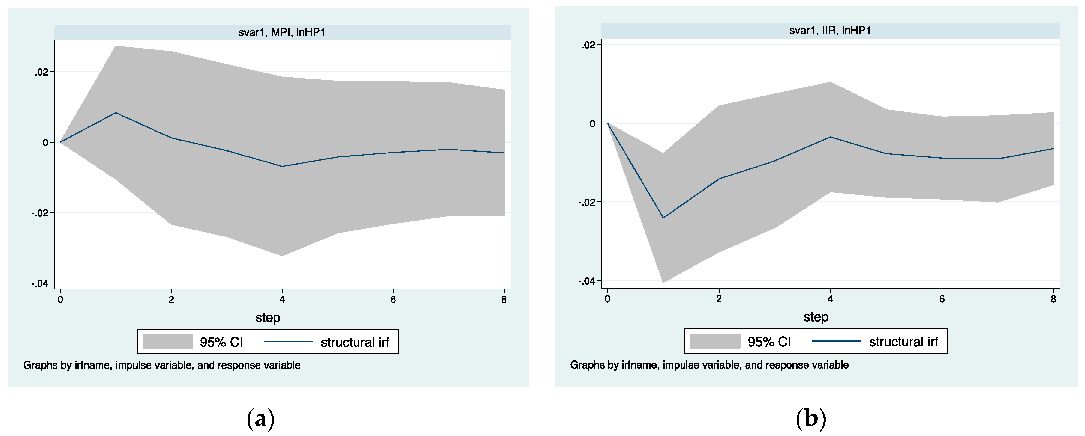
For the impulse response analysis, from Figure 4a, we can find that the impulse of macroprudential policy on housing prices is positive in the first period, then returns to around 0 in the second period and begins to turn negative, then reaches the peak of negative impact in the fourth period, and gradually decreases back to 0. This shows that macroprudential policy cannot restrain housing prices but can make it rise in the short run. As we mentioned in theoretical analysis, the reason is that tightening monetary policy and macroprudential policy at the same time might make households borrowing costs rise suddenly and households with adaptive expectations may think it will be more difficult and expensive to borrow money in the future, so they choose to immediately raise funds to buy houses, which causes a short-term rise in housing prices. From Figure 4b, we can find that the impulse of monetary policy on housing prices is negative and reaches its peak in the first period, then gradually decreases to 0. This shows that monetary policy can restrain housing prices effectively and lastingly.
From Figure 5, we can see the interaction between monetary policy and macroprudential policy. Both monetary policy and macroprudential policy have a negative impulse on each other and reach a peak in the first period. This suggests that, in the short term, monetary policy and macroprudential policy may offset one another when it comes to regulating housing prices, which is consistent with our conclusion from Figure 4.
For the variance decomposition analysis, from Table 5, we can find that the change of housing prices is mainly due to its own impact, and the proportion of it has always remained above 50%. This once again proves the pro-cyclical nature and continuity of finance. The proportion of macroprudential policy impact on housing prices is only about 5%, and the proportion of monetary policy impact is between 35% and 40%. Moreover, from Figure 5b, monetary policy always has a negative impact on macroprudential policy, which indicates that macroprudential policy is not applicable to the regulation of housing prices, so the regulation of housing prices should be dominated by monetary policy.
Stock Prices
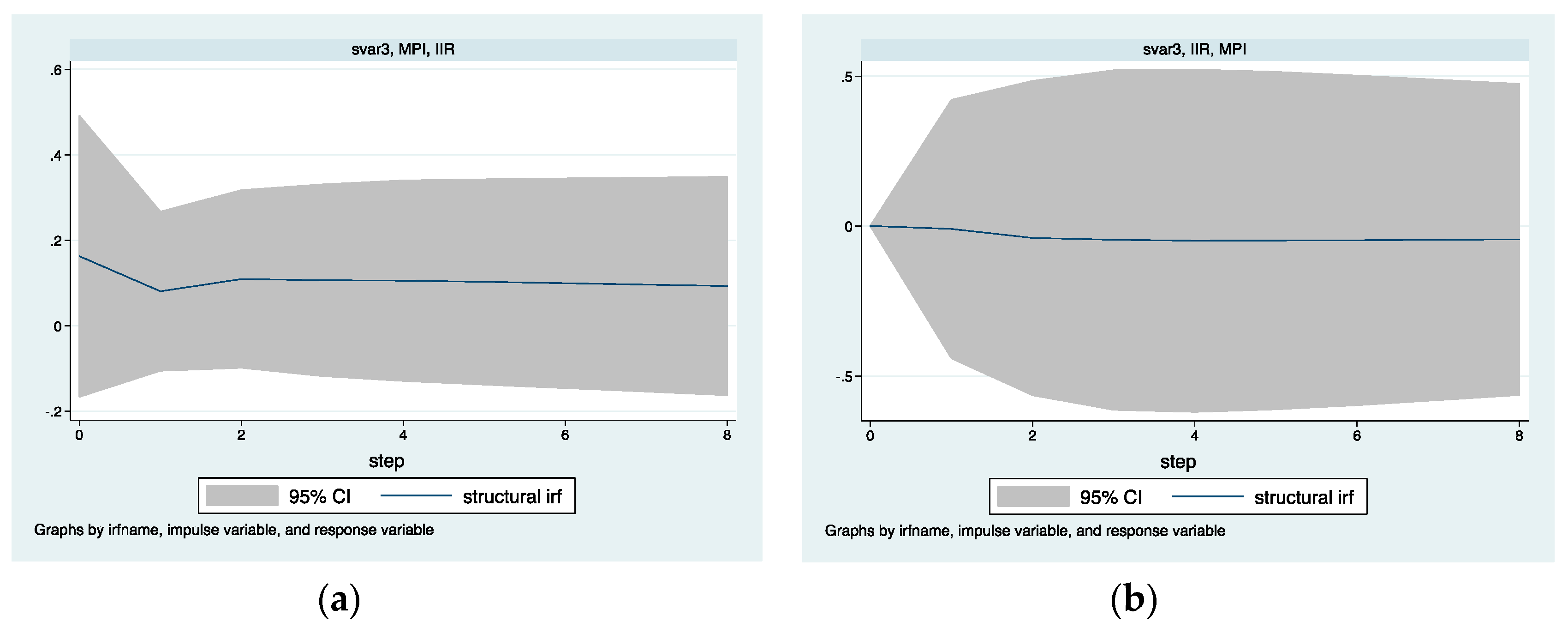
For the impulse response analysis, from Figure 6a, we can find that the impulse of macroprudential policy on stock prices is negative and reaches a peak in the first period, then gradually weakens and lasts for a long time. This shows that macroprudential policy can regulate the stock prices, especially the stock price bubbles effectively. From Figure 6b, we can find that the impulse of monetary policy on stock prices is only negative in the first period, where the possible amplitude is large, then rapidly decreases to 0 in the second period. This shows that when regulating stock prices, monetary policy is maybe too strong and not sustainable, which may lead to large stock market volatility.
For the interaction between macroprudential policy and monetary policy, from Figure 7, we can find macroprudential policy has a positive impulse on monetary policy, while monetary policy has little impact on macroprudential policy.
For the variance decomposition analysis, from Table 6, we can find that the change of stock price is also mainly due to the impact of itself, the proportion of which still remains above 80% in the eighth period. This shows that the stock market is more pro-cyclical and continuous than the housing market. The proportion of macroprudential policy impact on stock prices gradually increases and exceeds 15% in the eighth period, while the proportion of monetary policy impact is only around 2%. Moreover, considering the effects of the two kinds of policies on stock prices and their interaction, we believe that macroprudential policy, which has a moderate and lasting effects and is relatively independent, should play a leading role in regulating stock prices.
4.4. Robustness Check
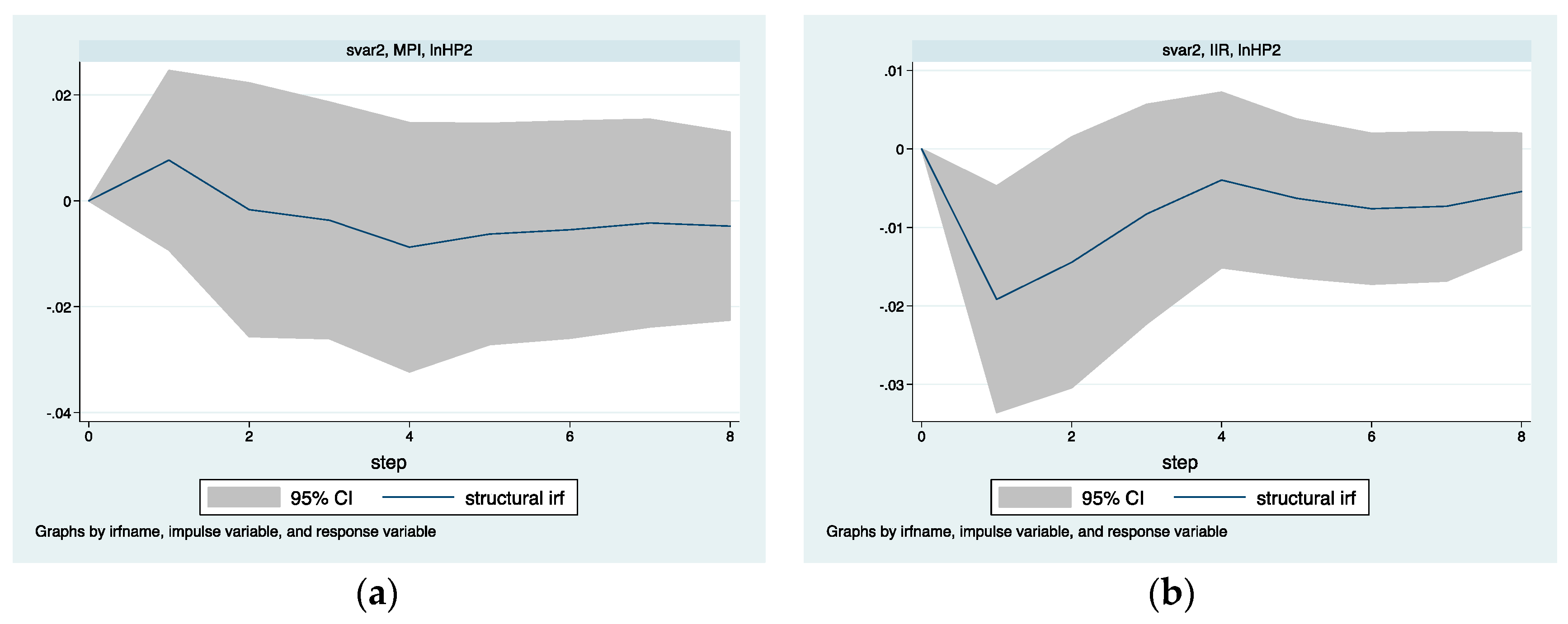
In order to ensure the robustness and accuracy of estimation results, we replace some variables and re-estimate the models. In the analysis of bank risk-taking, we select the impaired loan ratio (ILR) as the variable for risk-taking. In the analysis of asset prices, we select the logarithm of average price of commercial housing (lnHP2) as the variable for housing prices and growth rate of Shanghai Composite Index (SI) as the variable for stock prices. The results are shown in Table 7 and Figure 8 and Figure 9. In order to highlight the focus of the study, we do not report the estimation results of control variables and constant in bank risk-taking analysis, and do not report the interaction between monetary policy and macroprudential policy in asset prices analysis.
From Table 7, Figure 8 and Figure 9, we can find that whether from the System GMM analysis of the impact of monetary policy and macroprudential policy on bank risk-taking or the SVAR analysis of the impact on asset prices, the results of the robustness check are almost identical with the estimated results in the empirical analysis, which once again demonstrates the robustness and accuracy of estimation results.
5. Conclusions
This paper provides a theoretical analysis and China’s empirical evidence on the impact of monetary policy and macroprudential policy coordination on financial stability and sustainability. Financial stability and sustainability are important guarantees for sound economic development. Macroprudential policy is mainly used to prevent systemic risks and can play a role in specific industries and sectors, while monetary policy is mainly used to regulate aggregate demand and can play a role in all industries and sectors. Monetary policy and macroprudential policy can affect bank risk-taking and asset prices through some similar channels, such as the credit channel and the balance sheet channel. Because both policies have some side effects and sometimes conflict with each other, they cannot be implemented independently. Financial stability and sustainability can only be achieved if the two policies are aligned with each other for achieving different regulating objectives. Combined with the results of our theoretical and empirical analysis, we come to the following conclusions.
Firstly, for regulating bank risk-taking, monetary policy and macroprudential policy should conduct counter-cyclical regulation simultaneously. The proportion of indirect financing is larger than that of direct financing in China at the present stage, and corporate financing mainly relies on bank credit, so bank credit and risk-taking have an important impact on China’s financial and economic stability. During an economic boom, faced with the strong demand for credit, banks tend to lower the credit standard and expand the credit quantity, thus taking excessive risks; while in an economic depression, banks may reduce the credit for fear of taking risks, further weakening economic growth and slowing recovery. According to our empirical results, monetary policy and macroprudential policy promote each other in the regulation of bank risk-taking, and macroprudential policy has certain monetary policy effects. Therefore, monetary policy and macroprudential policy should conduct counter-cyclical regulation simultaneously. During an economic boom, monetary policy and macroprudential policy should be tightened at the same time. For example, while interest rates are being raised through open market operation or other monetary policy tools, the buffer capital and provision withdrawal of commercial banks should be increased through the countercyclical capital buffer policy and dynamic provision policy, and the bank capital asset ratio policy should be tightened to restrict bank credit expansion, thus preventing banks from excessive credit and excessive risk. In an economic depression, loose monetary policy and macroprudential policy should be implemented to release liquidity and increase the supply of credit. Since monetary policy has zero lower bound, when nominal interest rates fall to around zero and monetary policy cannot further stimulate economy, macroprudential policy can make up for this defect and continue to use capital buffers to release liquidity and accelerate economic recovery. If monetary policy and macroprudential policy are not synchronized, policy failures could occur. For example, during an economic boom, only increasing the rate of deposit reserve through monetary policy while loosening bank capital assets ratio constraints will not curb the expansion of bank credit, because banks can meet the requirements of the deposit reserve rate only by increasing the deposit. But if bank capital assets ratio constraints are tightened at the same time, banks must reduce the proportion of risk assets, thus reducing lending. It is also important to note that macroprudential tools should be coordinated, e.g., in an economic depression, raising the loan-to-value ratio should be accompanied by loosening banks’ capital asset ratio. Otherwise, although households and companies can borrow more, banks are not able to supply more loans [39]. In addition, macroprudential policy should pay more attention to the level of risk-taking of systemically important financial institutions, because these financial institutions have a significant influence on the entire financial system. If they go bankrupt due to excessive risk-taking, there would be a great damage to the entire financial system.
Secondly, for regulating housing prices, tight monetary policy and tight macroprudential policy should be implemented alternately. Over the past 10 years, the continuous rise of housing prices in China has not only driven the rapid economic growth, but also made a large number of funds leave real economy sectors and flood into the real estate industry. The flood of money has further reinforced people’s expectation that housing prices will rise. As a result, the investment demand for housing exceeds the rigid living demand, thus exacerbating the risk of housing price bubbles. Controlling the rising trend of housing price is the key to prevent the outbreak of housing price bubble risk. Our empirical results show that both monetary policy and macroprudential policy can control the rise of housing prices in the long run, but the simultaneous tightening of the two policies will result in the rise of housing prices in the short run. Therefore, when controlling the housing price, the tightening monetary policy should be first used to raise the interest rate, thus increasing the cost of borrowing money, so as to reduce the investment demand and speculative demand for housing. At the same time, the tight monetary policy can send a signal to curb people’s expectation of continuous rise of housing prices. When tightening monetary policy, policy makers should loosen macroprudential policy at the beginning to maintain the availability of credit, so as to avoid the large demand for housing in the short run caused by people’s expectation that credit cost will continue to rise in the future due to the tightening of both policies. After the implementation of tight monetary policy for 3–4 years, its impact on housing prices tends to flatten out. At this time, it is necessary to tighten macroprudential policy, such as raising bank capital requirements to restrict credit and raising the down payment ratio to reduce household leverage, thus further controlling housing prices. At the same time, the loan-to-value ratio constraints can be strengthened to enable banks to exclude borrowers with low repayment ability without increasing the borrowing cost of households, thus reducing the probability of housing price bubble bursting. Such an alternative policy combination can keep housing prices stable for a long time.
Thirdly, for regulating stock price bubbles, macroprudential policy should be the first defense-line and monetary policy should be the second one. In recent years, a large number of funds have been idling in the capital market for profit, which makes the capital market, especially the stock market, very sensitive to the policy interest rate. A small change in the policy interest rate will cause a large stock price fluctuation. At the same time, according to the rational expectation hypothesis, the implementation of monetary policy will make the public have the expectation of the policy effect based on the information they have, thus affecting the investor sentiment. For instance, the implementation of a tight monetary policy in order to control the bubble of stock prices will make investors expect that the stock market will go down in the future, so they choose to withdraw funds from the stock market, and large-scale withdrawal of funds will strengthen the panic of investors and further cause the stock market crash. It can be seen that monetary policy has a dramatic impact on stock prices, which is also shown in our empirical results. Therefore, monetary policy is not the optimal choice to regulate stock price bubbles. However, macroprudential policy controls the fund source of stock price bubbles only by affecting the access of credit funds into the stock market, which has little impact on the real economy. At the same time, we can see from our empirical results that the impact of macroprudential policy on stock prices is moderate and lasting, so it can serve as the first defense-line against the risk of stock price bubbles. For instance, strengthening the information disclosure to keep the stock price from deviating from the real value of the enterprise and help it stay within a reasonable range; raising the capital asset ratio of banks to prevent excessive credit expansion and reduce the occurrence of high-risk behavior of investing through credit; tightening loan-to-value constraint to reduce the amount of loans available to enterprises and households and reduce the likelihood of investing via mortgages. In a general way, monetary policy is not used to regulate the stock market. But when macroprudential policy fails to regulate the stock market, monetary policy should be the second line of defense against the risk of stock price bubbles. Once monetary policy is tightened to prevent the risk of stock price bubbles, a loose macroprudential policy should be implemented at the same time to maintain sufficient liquidity, stabilize market sentiment, and prevent the stock price from fluctuating dramatically. For example, while interest rates are raised, the capital asset ratio of banks should be loosened, and the loan-to-value ratio upper limit should be raised.
Additionally, from the practice of maintaining financial stability and sustainability through coordination between monetary policy and macroprudential policy, we can find that apart from the coordination of the two policies’ direction, the coordination of the two policies’ intensity is also of great importance. If the intensity of the two policies is not coordinated properly, it is not only impossible to achieve the expected regulation goal, but also possible to cause policy overshoot and reduce social welfare. This will be our next research direction.
Author Contributions
Conceptualization, Y.J. and C.L.; methodology, Y.J. and C.L.; software, C.L., J.Z. and X.Z.; formal analysis, Y.J. and C.L.; data curation, J.Z. and X.Z.; writing—original draft preparation, C.L., J.Z. and X.Z.; writing—review and editing, Y.J., C.L., J.Z. and X.Z.; supervision, Y.J.
Funding
This research was funded by The National Social Science Fund of China (Major Project), grant number 16ZDA037; China Scholarship Council, grant number 201806240131; Sichuan Provincial Education Department Humanities and Social Science Key Research Base Sichuan National Mountain Economic Development Research Center Fund, grant number SDJJ1817 and Sichuan Electronic Commerce and Modern Logistics Research Center Fund, grant number DSWL18-3.
Acknowledgments
Special thanks go to Professor Edward Tower for the guidance and help to Chong Li during his study at Duke University. Thanks go to Michael Guesev for the meticulous revisions and comments. The authors also would like to thank the editors and anonymous referees sincerely for their kind help and valuable comments on the paper.
Conflicts of Interest
The authors declare no conflict of interest.
References
- Zhang, Q. Discussion on Financial Stability and the Functions of the Central Bank. Doctoral Thesis, Dongbei University of Finance and Economics, Dalian, China, December 2006. [Google Scholar]
- Wellink, N. Central Banks as Guardians of Financial Stability. In Proceedings of the seminar “Current Issues in Central Banking”, Oranjestad, Aruba, 14 November 2002. [Google Scholar]
- Foot, M. What Is Financial Stability and How Do We Get It? In Proceedings of the Roy Bridge Memorial Lecture, London, UK, 3 April 2003. [Google Scholar]
- Bernanke, B.S.; Gertler, M.; Gilchrist, S. The Financial Accelerator and the Flight to Quality. Rev. Econ. Stat. 1996, 78, 1–15. [Google Scholar] [CrossRef]
- Crockett, A. The theory and practice of financial stability. De Economist 1996, 144, 531–568. [Google Scholar] [CrossRef]
- Ferguson, R.W. Should financial stability be an explicit central bank objective. In Challenges to Central Banking from Globalized Financial Systems, 1st ed.; Ugolini, P., Schaechter, A., Stone, M.R., Eds.; International Monetary Fund: Washington, DC, USA, 2003; Volume 12, pp. 208–223. [Google Scholar]
- Taylor, J.B. Discretion versus Policy Rules in Practice. In Carnegie-Rochester Conference Series on Public Policy; North-Holland: Amsterdam, The Netherlands, 1993. [Google Scholar]
- Bernanke, B.S.; Gertler, M. Should central banks respond to movements in asset prices? Am. Econ. Rev. 2001, 91, 253–257. [Google Scholar] [CrossRef]
- Lehar, A. Measuring systemic risk: A risk management approach. J. Bank. Financ. 2005, 29, 2577–2603. [Google Scholar] [CrossRef] [Green Version]
- Wang, X.; Li, J. The relationship between monetary policy and macroprudential regulation under the financial stability objective: A literature review. Stud. Int. Financ. 2013, 4, 22–29. [Google Scholar]
- Guo, Z.; Zhang, M. Coordinated use of monetary and macroprudential policies. Economist 2017, 5, 68–75. [Google Scholar]
- Zhong, Z. Research review on macroprudential regulation. Econ. Theory Bus. Manag. 2012, 7, 49–55. [Google Scholar]
- FSB, IMF, BIS. Macroprudential Policy Tools and Frameworks, Update to G20 Finance Ministers and Central Bank Governors. Unpublished. Available online: https://www.imf.org/external/np/g20/pdf/021411.pdf (accessed on 10 January 2019).
- Galati, G.; Moessner, R. Macroprudential policy—A literature review. J. Econ. Surv. 2013, 27, 846–878. [Google Scholar]
- Borio, C.; Drehmann, M. Assessing the risk of banking crises–revisited. BIS Q. Rev. 2009, 3, 29–46. [Google Scholar]
- Caruana, J. Macroprudential policy: Working towards a new consensus. In Proceedings of the Emerging Framework for Financial Regulation and Monetary Policy High-level Meeting, Washington DC, USA, 23 April 2010. [Google Scholar]
- N’Diaye, P. Countercyclical Macro Prudential Policies in a Supporting Role to Monetary Policy; IMF Working Paper; IMF: Washington, DC, USA, 2009; Volume 9, pp. 1–22. [Google Scholar]
- Lambertini, L.; Mendicino, C.; Punzi, M.T. Leaning against boom–bust cycles in credit and housing prices. J. Econ. Dyn. Control 2013, 37, 1500–1522. [Google Scholar] [CrossRef] [Green Version]
- Cecchetti, S. On the similarities of capital adequacy and monetary policy. In Proceedings of the Thirteenth Annual Conference of the Central Bank of Chile, Santiago, Chile, 19 November 2009. [Google Scholar]
- Rubio, M.; Carrasco-Gallego, J.A. The new financial regulation in Basel III and monetary policy: A macroprudential approach. J. Financ. Stab. 2016, 26, 294–305. [Google Scholar] [CrossRef]
- Beau, D.; Clerc, L.; Mojon, B. Macro-Prudential Policy and the Conduct of Monetary Policy; Working Paper; Banque de France: Paris, France, 2012; Volume 390, pp. 1–32. [Google Scholar]
- Luo, N.; Cheng, F. Analysis of coordination effect of macroprudential policy and monetary policy on housing price fluctuation: Based on DSGE model of New Keynesianism. Stud. Int. Financ. 2017, 1, 39–48. [Google Scholar]
- Fang, Y.; Zhao, S.; Xie, X. Analysis on bank risk-taking of monetary policy and on coordination between monetary policy and macroprudential policy. Manag. World. 2012, 11, 9–19. [Google Scholar]
- Borio, C.; Zhu, H. Capital regulation, risk-taking and monetary policy: A missing link in the transmission mechanism? J. Financ. Stab. 2012, 8, 236–251. [Google Scholar] [CrossRef] [Green Version]
- Rajan, R.G. Has finance made the world riskier? Eur. Financ. Manag. 2006, 12, 499–533. [Google Scholar] [CrossRef]
- Adrian, T.; Shin, H.S. Money, liquidity, and monetary policy. Am. Econ. Rev. 2009, 99, 600–605. [Google Scholar] [CrossRef]
- Gu, H.; Zhang, Y. Monetary policy and real estate price control: Theory and Chinese experience. Econ. Res. J. 2014, 12, 29–44. [Google Scholar]
- Cerutti, E.; Claessens, S.; Laeven, L. The use and effectiveness of macroprudential policies: New evidence. J. Financ. Stab. 2017, 28, 203–224. [Google Scholar] [CrossRef]
- Laeven, L.; Levine, R. Bank governance, regulation and risk taking. J. Financ. Econ. 2009, 93, 259–275. [Google Scholar] [CrossRef] [Green Version]
- Altunbas, Y.; Gambacorta, L.; Marques-Ibanez, D. Do bank characteristics influence the effect of monetary policy on bank risk? Econ. Lett. 2012, 117, 220–222. [Google Scholar] [CrossRef] [Green Version]
- Delis, M.D.; Kouretas, G.P. Interest rates and bank risk-taking. J. Bank. Financ. 2011, 35, 840–855. [Google Scholar] [CrossRef] [Green Version]
- Zhang, X.; Li, F.; Li, Z.; Xu, Y. Macroprudential Policy, Credit Cycle, and Bank Risk-Taking. Sustainability 2018, 10, 3620. [Google Scholar] [CrossRef]
- Blundell, R.; Bond, S. Initial conditions and moment restrictions in dynamic panel data models. J. Econ. 1998, 87, 115–143. [Google Scholar] [CrossRef] [Green Version]
- Claessens, S.; Valencia, F. The Interaction between Monetary and Macroprudential Policies. Unpublished. Available online: https://voxeu.org/article/interaction-between-monetary-and-macroprudential-policies (accessed on 10 January 2019).
- Xu, C.; Ai, X. Coordination of monetary policy and macro-prudential policy: An empirical research based on micro-data of China’s commercial banks. Jiangxi Soc. Sci. 2018, 6, 39–47. [Google Scholar]
- Jiang, H.; Zhang, X.; Shao, X.; Bao, J. How Do the Industrial Structure Optimization and Urbanization Development Affect Energy Consumption in Zhejiang Province of China? Sustainability 2018, 10, 1889. [Google Scholar] [CrossRef]
- Sims, C.A. Macroeconomics and reality. Econometrica 1980, 48, 1–48. [Google Scholar] [CrossRef]
- Chen, Q. Advanced Econometrics and Stata Application, 2nd ed.; Higher Education Press: Beijing, China, 2014; pp. 494–495. [Google Scholar]
- Hong, H.; Chen, Y.; Xiang, Y. Research on the influence of macroprudential management mechanism on monetary policy. Stud. Int. Financ. 2018, 9, 45–55. [Google Scholar]
Figure 1.
The relationship between loan growth and interest rate in China. Source: Wind Database.

Figure 2.
The channel through which monetary policy affects housing prices.

Figure 3.
The channel through which monetary policy affects the stock prices.

Figure 4.
The response of housing prices to macroprudential and monetary policies’ impulse. (a) is macroprudential policy’s impulse; (b) is monetary policy’s impulse.
Figure 4.
The response of housing prices to macroprudential and monetary policies’ impulse. (a) is macroprudential policy’s impulse; (b) is monetary policy’s impulse.

Figure 5.
The interaction of monetary policy and macroprudential and policy. (a) is monetary policy’s response to macroprudential policy’s impulse; (b) is macroprudential policy’s response to monetary policy’s impulse.
Figure 5.
The interaction of monetary policy and macroprudential and policy. (a) is monetary policy’s response to macroprudential policy’s impulse; (b) is macroprudential policy’s response to monetary policy’s impulse.

Figure 6.
The response of stock prices to macroprudential and monetary policies’ impulse. (a) is macroprudential policy’s impulse; (b) is monetary policy’s impulse.
Figure 6.
The response of stock prices to macroprudential and monetary policies’ impulse. (a) is macroprudential policy’s impulse; (b) is monetary policy’s impulse.

Figure 7.
The interaction of monetary policy and macroprudential and policy. (a) is monetary policy’s response to macroprudential policy’s impulse; (b) is macroprudential policy’s response to monetary policy’s impulse.
Figure 7.
The interaction of monetary policy and macroprudential and policy. (a) is monetary policy’s response to macroprudential policy’s impulse; (b) is macroprudential policy’s response to monetary policy’s impulse.

Figure 8.
The robustness check of housing prices impulse response results. (a) is macroprudential policy’s impulse; (b) is monetary policy’s impulse.
Figure 8.
The robustness check of housing prices impulse response results. (a) is macroprudential policy’s impulse; (b) is monetary policy’s impulse.

Figure 9.
The robustness check of stock prices impulse response results. (a) is macroprudential policy’s impulse; (b) is monetary policy’s impulse.
Figure 9.
The robustness check of stock prices impulse response results. (a) is macroprudential policy’s impulse; (b) is monetary policy’s impulse.


Table 1.
Control variables description.
| Variable | Definition | Data Source |
|---|---|---|
| Bank level | ||
| lnTA | The logarithm of total asset, used to measure size of a bank | Bank Focus database |
| ROAA | Return on average asset, used to measure profitability of a bank | Bank Focus database |
| EQR | Equity ratio = equity/total asset, used to measure the stability of a bank | Bank Focus database |
| LIR | Liquidity ratio = liquid asset/liquid liability, used to measure the liquidity of a bank | Bank Focus database |
| Macro level | ||
| GDP | GDP growth rate | CEInet Statistics database |
| CPI | CPI growth rate | CEInet Statistics database |
| FAI | Fixed asset investment growth rate | CEInet Statistics database |
Table 2.
The descriptive statistics of all the variables.
| Variable | Mean | Std. Dev. | Min | Max |
|---|---|---|---|---|
| RAR | 47.57211 | 12.23516 | 13.066 | 88.148 |
| ILR | 1.964337 | 3.318552 | 0 | 41.86 |
| MPI | 6.2 | 2.56222 | 2 | 11 |
| IIR | 2.441333 | 0.787571 | 1.24 | 4.16 |
| TA | 6046043 | 3.74 × 10⁷ | 6568 | 5.66 × 10⁸ |
| ROAA | 0.8728757 | 0.5967919 | −6.533 | 2.635 |
| EQR | 8.885968 | 7.882939 | −13.714 | 94.709 |
| LIR | 30.37318 | 19.33732 | 2.454 | 182.436 |
| GDP | 9.406667 | 2.150688 | 6.7 | 14.2 |
| CPI | 2.616 | 1.697813 | −0.69 | 5.86 |
| FAI | 19.89664 | 7.63802 | 5.733668 | 29.95478 |
| HP1 | 4717.499 | 1691.157 | 2197 | 7614 |
| HP2 | 4994.563 | 1742.648 | 2359 | 7892 |
| SPE | 22.63933 | 12.67276 | 10.99 | 59.24 |
| SI | 16.34594 | 51.57657 | −65.3941 | 130.4334 |
Table 3.
The separate impact of monetary policy and macroprudential policy on commercial banks risk-taking.
Table 3.
The separate impact of monetary policy and macroprudential policy on commercial banks risk-taking.
| System GMM | OLS-Robust | System GMM | OLS-Robust | |
|---|---|---|---|---|
| Variable | RAR | RAR | RAR | RAR |
| L.RAR | 0.660 *** | 0.808 *** | 0.659 *** | 0.806 *** |
| (0.0243) | (0.0221) | (0.0254) | (0.0226) | |
| IIR | −0.636 *** | −0.344 | ||
| (0.0626) | (0.242) | |||
| MPI | −0.360 *** | −0.133 | ||
| (0.0620) | (0.194) | |||
| L.lnTA | −0.162 *** | 0.115 | −0.0658 ** | 0.118 |
| (0.0409) | (0.0954) | (0.0301) | (0.0959) | |
| L.ROAA | −2.905 *** | −0.473 | −3.008 *** | −0.546 |
| (0.273) | (0.421) | (0.305) | (0.422) | |
| L.EQR | −0.382 *** | −0.123 ** | −0.312 *** | −0.115 ** |
| (0.0326) | (0.0526) | (0.0307) | (0.0528) | |
| L.LIR | 0.114 *** | −0.0228 | 0.0917 *** | −0.0279 |
| (0.00624) | (0.0178) | (0.00750) | (0.0178) | |
| GDP | 0.281 *** | 0.249 * | 0.0514 | 0.188 |
| (0.0564) | (0.132) | (0.0618) | (0.185) | |
| CPI | −0.463 *** | −0.532 *** | −0.513 *** | −0.569 *** |
| (0.0289) | (0.118) | (0.0335) | (0.114) | |
| FAI | 0.0820 *** | 0.0730 ** | 0.0755 *** | 0.0703 * |
| (0.0131) | (0.0325) | (0.0130) | (0.0373) | |
| Constant | 18.42 *** | 7.667 *** | 20.71 *** | 8.599 ** |
| (0.771) | (2.231) | (1.707) | (3.637) | |
| AR (1) | 0.0000 | 0.0000 | ||
| AR (2) | 0.8789 | 0.7246 | ||
| Wald Test | 4776.97 *** | 6866.90 *** | ||
| Sargan Test | 0.2300 | 0.1873 | ||
| Observations | 842 | 842 | 842 | 842 |
| R-squared | 0.772 | 0.772 | ||
| Number of bank | 88 | 88 |
Notes: standard errors in parentheses, *** presents p < 0.01, ** presents p < 0.05, * presents p < 0.1. Source: author’s calculation.
Table 4.
The impact of monetary policy and macroprudential policy on commercial banks risk-taking and the interaction between two policies.
Table 4.
The impact of monetary policy and macroprudential policy on commercial banks risk-taking and the interaction between two policies.
| System GMM | OLS-Robust | System GMM | OLS-Robust | |
|---|---|---|---|---|
| Variable | RAR | RAR | RAR | RAR |
| L.RAR | 0.649 *** | 0.807 *** | 0.663 *** | 0.814 *** |
| (0.0258) | (0.0226) | (0.0280) | (0.0221) | |
| IIR | −0.587 *** | −0.323 | −8.400 *** | −9.401 *** |
| (0.0725) | (0.249) | (0.557) | (1.498) | |
| MPI | −0.210 *** | −0.0718 | −3.286 *** | −3.771 *** |
| (0.0741) | (0.200) | (0.216) | (0.633) | |
| IIR*MPI | 1.123 *** | 1.323 *** | ||
| (0.0718) | (0.215) | |||
| L.lnTA | −0.0910 *** | 0.118 | 0.172 *** | 0.174 * |
| (0.0327) | (0.0959) | (0.0437) | (0.0943) | |
| L.ROAA | −2.832 *** | −0.489 | −2.154 *** | −0.174 |
| (0.286) | (0.424) | (0.278) | (0.418) | |
| L.EQR | −0.333 *** | −0.121 ** | −0.322 *** | −0.121 ** |
| (0.0338) | (0.0530) | (0.0407) | (0.0518) | |
| L.LIR | 0.101 *** | −0.0239 | 0.142 *** | −0.00839 |
| (0.00899) | (0.0181) | (0.00907) | (0.0179) | |
| GDP | 0.153 ** | 0.202 | 0.225 *** | 0.120 |
| (0.0630) | (0.185) | (0.0654) | (0.182) | |
| CPI | −0.438 *** | −0.527 *** | −0.308 *** | −0.341 *** |
| (0.0310) | (0.119) | (0.0344) | (0.120) | |
| FAI | 0.0670 *** | 0.0664 * | −0.0765 *** | −0.116 ** |
| (0.0134) | (0.0374) | (0.0199) | (0.0471) | |
| Constant | 20.77 *** | 8.699 ** | 37.42 *** | 34.86 *** |
| (1.750) | (3.636) | (2.248) | (5.550) | |
| AR (1) | 0.0000 | 0.0000 | ||
| AR (2) | 0.9808 | 0.8207 | ||
| Wald Test | 6379.19 *** | 4916.48 *** | ||
| Sargan Test | 0.1992 | 0.3067 | ||
| Observations | 842 | 842 | 842 | 842 |
| R-squared | 0.772 | 0.782 | ||
| Number of bank | 88 | 88 |
Notes: standard errors in parentheses, *** presents p < 0.01, ** presents p < 0.05, * presents p < 0.1. Source: author’s calculation.
Table 5.
The variance decomposition of housing prices.
| Period | lnHP1 | MPI | IIR |
|---|---|---|---|
| 1 | 1 | 0 | 0 |
| 2 | 0.581332 | 0.044523 | 0.374145 |
| 3 | 0.568878 | 0.035673 | 0.395449 |
| 4 | 0.556743 | 0.035667 | 0.407589 |
| 5 | 0.588554 | 0.050631 | 0.360815 |
| 6 | 0.584151 | 0.054451 | 0.361398 |
| 7 | 0.58004 | 0.05404 | 0.365919 |
| 8 | 0.570029 | 0.052932 | 0.377039 |
Table 6.
The variance decomposition of stock prices.
| Period | SPE | MPI | IIR |
|---|---|---|---|
| 1 | 1 | 0 | 0 |
| 2 | 0.94139 | 0.038106 | 0.020504 |
| 3 | 0.918468 | 0.061178 | 0.020354 |
| 4 | 0.895587 | 0.084509 | 0.019904 |
| 5 | 0.875424 | 0.105136 | 0.019441 |
| 6 | 0.85722 | 0.123719 | 0.019061 |
| 7 | 0.840871 | 0.140384 | 0.018745 |
| 8 | 0.826154 | 0.155374 | 0.018471 |
Table 7.
The robustness check results of bank risk-taking.
| System GMM | System GMM | System GMM | System GMM | |
|---|---|---|---|---|
| Variable | ILR | ILR | ILR | ILR |
| L.ILR | 0.692 *** | 0.705 *** | 0.691 *** | 0.665 *** |
| (0.00281) | (0.00442) | (0.00415) | (0.00386) | |
| IIR | −0.0485 *** | −0.0313 *** | −0.885 *** | |
| (0.00362) | (0.00386) | (0.0225) | ||
| MPI | −0.0494 *** | −0.0431 *** | −0.379 *** | |
| (0.00373) | (0.00401) | (0.00892) | ||
| IIR*MPI | 0.122 *** | |||
| (0.00323) | ||||
| Control Variables | control | control | control | control |
| AR (1) | 0.0048 | 0.0045 | 0.0045 | 0.0045 |
| AR (2) | 0.6443 | 0.5989 | 0.6156 | 0.5395 |
| Wald Test | 248893 *** | 192068 *** | 328662 *** | 637334 *** |
| Sargan Test | 0.4006 | 0.4151 | 0.4331 | 0.2787 |
| Observations | 660 | 660 | 660 | 660 |
| Number of bank | 86 | 86 | 86 | 86 |
Notes: standard errors in parentheses, *** presents p < 0.01, ** presents p < 0.05, * presents p < 0.1. Source: author’s calculation.
© 2019 by the authors. Licensee MDPI, Basel, Switzerland. This article is an open access article distributed under the terms and conditions of the Creative Commons Attribution (CC BY) license (http://creativecommons.org/licenses/by/4.0/).
Share and Cite
MDPI and ACS Style
Jiang, Y.; Li, C.; Zhang, J.; Zhou, X. Financial Stability and Sustainability under the Coordination of Monetary Policy and Macroprudential Policy: New Evidence from China. Sustainability 2019, 11, 1616. https://doi.org/10.3390/su11061616
AMA Style
Jiang Y, Li C, Zhang J, Zhou X. Financial Stability and Sustainability under the Coordination of Monetary Policy and Macroprudential Policy: New Evidence from China. Sustainability. 2019; 11(6):1616. https://doi.org/10.3390/su11061616
Chicago/Turabian StyleJiang, Ying, Chong Li, Jizhou Zhang, and Xiaoyi Zhou. 2019. "Financial Stability and Sustainability under the Coordination of Monetary Policy and Macroprudential Policy: New Evidence from China" Sustainability 11, no. 6: 1616. https://doi.org/10.3390/su11061616
Note that from the first issue of 2016, this journal uses article numbers instead of page numbers. See further details here.