Estimation of Housing Price Variations Using Spatio-Temporal Data


1
Department of Quantitative Methods for Economics and Business, University of Granada, 18011 Granada, Spain
2
Department of Mathematical Analysis, University of Granada, 18071 Granada, Spain
*
Author to whom correspondence should be addressed.
Sustainability 2019, 11(6), 1551; https://doi.org/10.3390/su11061551
Submission received: 7 February 2019
/
Revised: 8 March 2019
/
Accepted: 11 March 2019
/
Published: 14 March 2019
(This article belongs to the Special Issue Sustainability Challenges in Real Estate Markets and Urban Property Developments)
Abstract
:This paper proposes a hedonic regression model to estimate housing prices and the spatial variability of prices over multiple years. Using the model, maps are obtained that represent areas of the city where there have been positive or negative changes in housing prices. The regression-cokriging (RCK) method is used to predict housing prices. The results are compared to the cokriging with external drift (CKED) model, also known as universal cokriging (UCK). To apply the model, heterotopic data of homes for sale at different moments in time are used. The procedure is applied to predict the spatial variability of housing prices in multi-years and to obtain isovalue maps of these variations for the city of Granada, Spain. The research is useful for the fields of urban studies, economics, real estate, real estate valuations, urban planning, and for scholars.
1. Introduction
In the real estate field, multivariate spatial data models have been widely explored [1,2,3,4,5], while multivariate spatio-temporal data models have received relatively less attention. The hedonic regression model is used to make real estate valuations and to determine the characteristics that affect property prices [6]. Classical estimation methods, such as ordinary-least-squares (OLS), ignore the presence of spatial autocorrelation, since they assume the independence of the observations [7].
Two approaches are commonly used in spatial hedonic modeling: spatial econometrics [8] and the geostatistical approach [9]. Spatial econometrics uses the spatial weight matrix and requires an a priori specification of the matrix, which may affect the final results [10]. However, geostatistics is a method in which the variance–covariance matrix depends on the Euclidean distance [11]. In the case of spatial autocorrelation of the error terms, the spatial error model (SEM) is not better than the geostatistical approach [12]. The literature suggests that the kriging geostatistical method improves the prediction performance of spatial hedonic models [13]. Moreover, kriging models are superior to other methods (OLS, SEM, spatial lag model, etc.) in terms of their prediction accuracy [14].
Several methods that consider both spatial and temporal dependences that simultaneously affect housing prices have been proposed for the study of real estate. A classical method for considering time-fixed effects is to include dummy variables indicating the year a house is being sold [15,16]. The spatio-temporal autoregressive (STAR) model and its variations [17,18,19,20] is another method that consists of a spatio-temporal model based on a generalization of the traditional spatial autoregressive model (SAR) [21]. This method has also been used to analyze housing prices in Spain [22,23]. Several authors have used geographically and temporally weighted regression to capture spatial and temporal heterogeneity in real estate market data [24,25,26,27].
The cokriging method has been used to spatially relate housing prices with different auxiliary variables [28], age or central heating [29], and quality of the area [30]. A recent application of this method to housing prices can be found in Kuntz and Helbich [31], who consider structural and neighborhood characteristics as auxiliary variables. D’Agostino et al. [32], Fassò and Finazzi [33], and Joyner et al. [34] used the cokriging method to perform spatio-temporal studies in the fields of geology, the environment, and climatology, respectively, and to obtain isovalue maps of the variable of interest. Cokriging has also been used to estimate the temporal change in spatially-correlated variables between only two time instants [35] and for data irregularly distributed in space and time [36].
In this paper, a hedonic housing price model using the regression-cokriging method (RCK) is proposed in order to estimate a system of equations, in which each equation corresponds to a sample of dwellings taken in a different year. Each of these equations explains the selling price of a given year, and not all equations have the same explanatory variables. The main novelty of this work is that the proposed method solves a common problem for agencies and entities interested in estimating housing prices or spatio-temporal variations in prices when samples of dwellings in different locations (heterotopic data), or in the same location (isotopic data) taken at different points in time, are available.
There are suitable methods for spatio-temporal time modeling when sufficient information is available in both dimensions, and when data are both regularly and irregularly distributed in space or time (see [37,38,39,40,41]). Due to the limited availability of temporal information in this work, a discrete temporal study (multi-years) has been performed considering the cross-correlation of spatial data between different years rather than the dual structure of spatio-temporal autocorrelation. This lack of temporal information makes the methodology used in this work (RCK) particularly attractive, as this may occur when modeling other phenomena and in other regions where there is sufficient spatial information but a scarcity of temporal information. According to Papritz and Flühler [42], if the data consist of long time series at few sampling locations, then the spatio-temporal process can be modeled as a multivariate time series. However, if many observations are distributed in space at a few sampling times, then a multivariate spatial random process, such as a cokriging method, is a suitable simplification for the general space-time process. This method is suitable for estimating variations between different (discrete) moments, whether they are distributed regularly or irregularly in space or time. For instance, Gallois et al. [36] applied cokriging in two periods (winter and summer) and D’Agostino et al. [32] in three months (May, July and November) for irregularly distributed observations.
The aim of this work is twofold. First, the system of equations is estimated. Secondly, isovalue maps of housing price variations are obtained across the different time periods by modeling the spatial autocorrelation and cross-correlation over multi-years. These maps permit detection of areas where prices are falling, or, conversely, where they are rising.
The paper is structured as follows. The regression-cokriging method and the cokriging with external drift method, which is the multivariate generalization of the well-known kriging with external drift (KED) method, are first described. The main results of applying these methods to housing prices in Granada, Spain, for the period 1988–2005 are then presented.
2. Material and Methods
2.1. Regression-Cokriging Predictor
In this section, a predictor known as regression-cokriging is presented within the framework of geostatistics. To obtain this predictor, a multi-equation econometric model is used, in which the price of housing is the dependent variable in all the model equations, and the structural and location characteristics of the dwellings are the explanatory variables. In our case, each of the model equations contain different datasets for different years. It is assumed that the disturbances are spatially autocorrelated within each equation, and can also be spatio-temporally correlated between equations. In this regard, Gelfand et al. [43] developed a framework where spatial and temporal effects can be modeled in the error structure. The aim is to estimate the model parameters, predict housing prices in any part of the city, and estimate housing price variations between different years. When there is spatial independence, the best linear unbiased estimator (BLUE) is the ordinary least squares estimator (OLS). However, the presence of spatial dependence is common in the housing market because short-distance house prices are more alike than long-distance house prices. Due to the presence of correlation in the disturbances, the OLS estimator is inefficient. Therefore, general least square (GLS) is used to estimate the parameters of the model [7] and to carry out the predictions.
Let us take the following multi-equation model with spatial autocorrelation (see [44,45]):
where:
and where is a vector containing the prices of houses; j = 1, 2, …; q denotes the moment of time; is the vector of the coefficients of the j-th regression equation; is the matrix () of explanatory variables of the j-th regression equation; and are the disturbances presenting spatial autocorrelation, which can also be cross-correlated.
The GLS estimator of is BLUE:
where V is the covariance matrix of disturbances.
The best linear unbiased predictor (BLUP) of at a new location is [45]:
where: is the global drift model; is a matrix of the known characteristics of a house to be valued located at for each year j. is a matrix containing the covariances of the disturbances between houses and the house to be valued located at . In practice, the V and matrices are unknown, and can be estimated from the variogram function of residuals (see [46]).
Here, is the cokriging with external drift (CKED) predictor, which is a multivariable spatial predictor [45], also known as universal cokriging (UCK) [44,47] in the particular case where the matrix X contains only the trend of the process and is usually expressed by a linear combination of spatial coordinates. However, Pebesma [48] also refers to the case where the X matrix includes other explanatory variables as UCK. In the case of the single-equation model, and when the X matrix contains any type of explanatory variable, this predictor is called kriging with external drift (KED) or universal kriging (UK). As Hengl et al. [49] indicated, KED should give the same predictions as regression-kriging (RK), which is obtained by adding the drift plus ordinary kriging of residuals. In this paper, RK has been generalized to the multi-equation case and regression-cokriging (RCK) has been used:
where is the estimate of the disturbance by ordinary cokriging of residuals [30].
According to Hengl, Heuvelink, and Stein [49], the main advantage of RK is that it is a flexible method for modeling and mapping because it can be used in combination with other methods, such as generalized linear models (GLM) or generalized additive models (GAM), among others [50]. Hengl et al. [51] reported that although KED seems to be computationally more straightforward than RK, both need to estimate the variogram of residuals. A disadvantage of RK is that it is a two-step method. These advantages and drawbacks can be generalized to the RCK and CKED methods.
2.2. Direct and Cross-Correlation of Residuals
The direct variogram is used to study the spatial autocorrelation of residuals of each equation, while the cross-variogram is used to examine the spatial correlation across different years in order to include the temporal interactions.
The direct variogram measures spatial dependence of residuals in year t. An unbiased estimator of the variogram is [52]:
where , with being the locations; h is a distance vector; and is the number of distant point-pairs.
The cross-variogram measures the spatial cross-dependence of the residuals between year t and year t′. The classical cross-variogram estimator requires that and be available for each location (isotopic data). In our case, however, the available observations correspond to different dwellings at different moments in time and the observations are, therefore, heterotopic. When the observations are heterotopic, the pseudo-cross-variogram is used [45,53]:
It is necessary to fit the variogram model to the empirical direct variogram or cross-variogram to perform the estimations. To do so, the exponential model was used:
The model fit depends on three parameters: the nugget effect , range , and sill (), where is a partial sill. The nugget effect is a measure of spatial discontinuity. For the exponential model, the practical range a’ = 3a [54] was used. This is the distance at which the model reaches 95% of its sill, and sill is the value that the variogram model attains at that range. The linear model of coregionalization (LMC) has been used to fit an exponential model to each direct and cross-variogram [55,56].
3. Data and Case Study
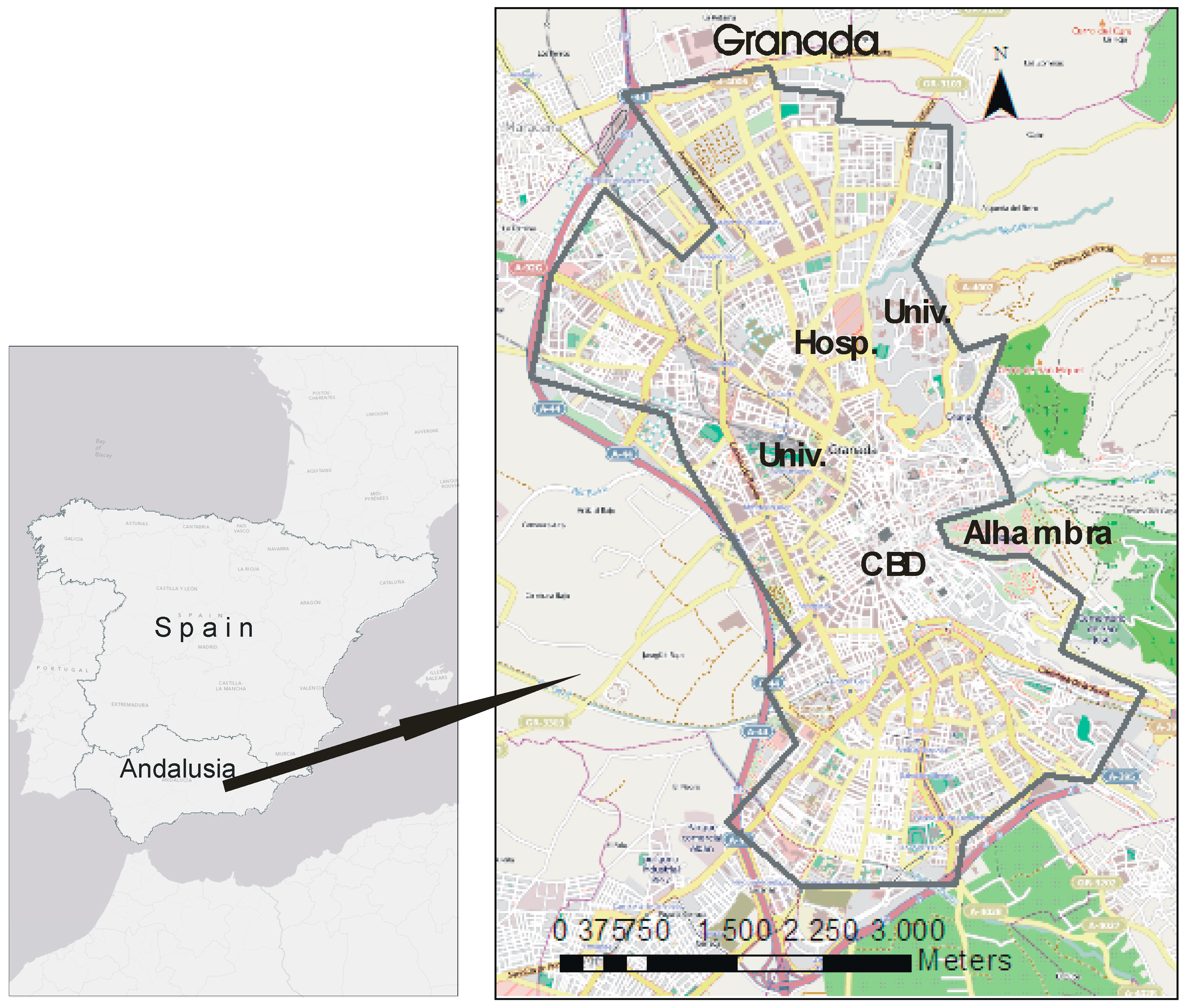
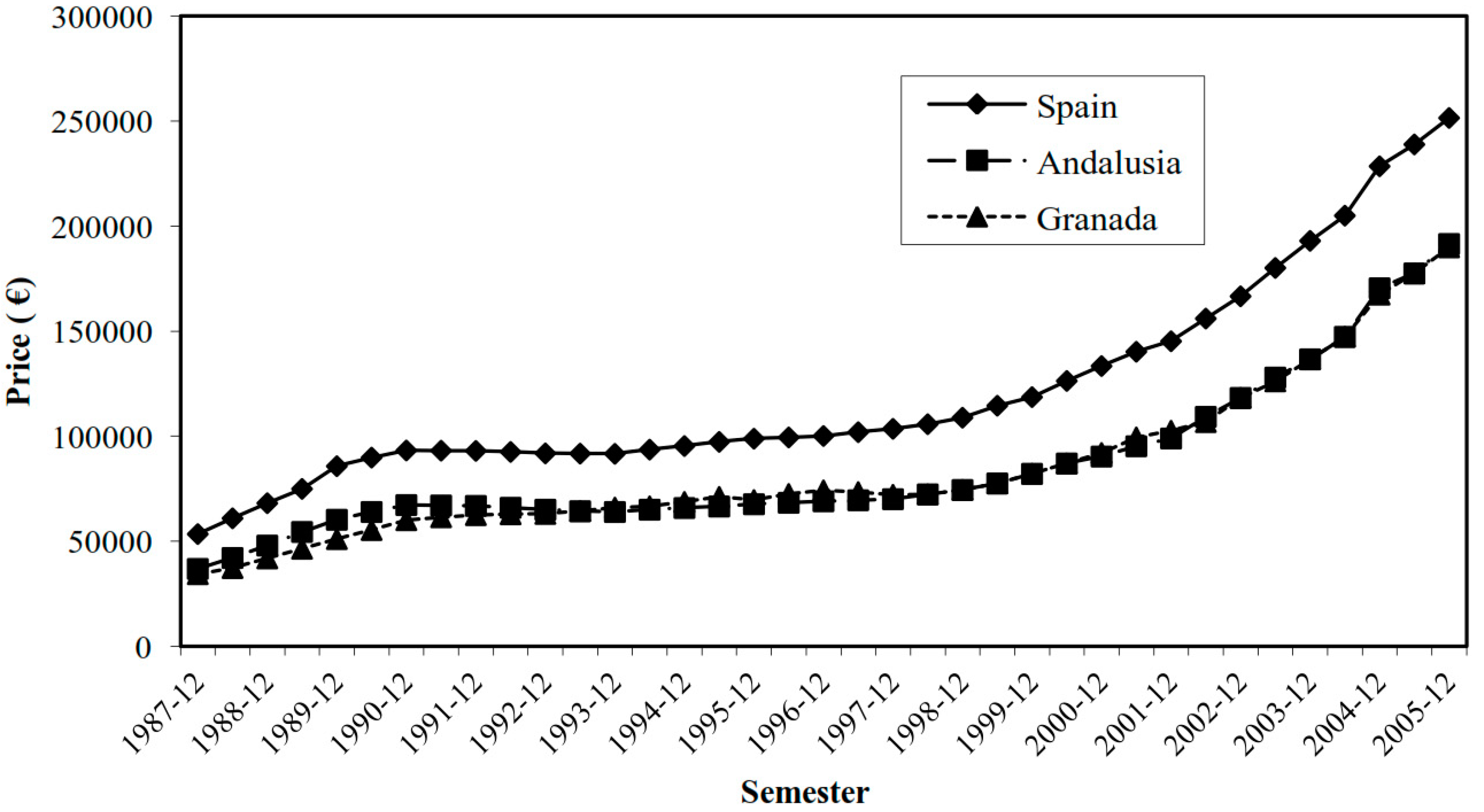
This work presents a hedonic regression model to explain spatial housing price variation in multi-years in the city of Granada, Spain. Granada is a small, historic city that is known worldwide for its monuments. It is located in southern Spain in the region of Andalusia (Figure 1). The study was carried out for the years 1988, 1991, 1995, and 2005. An overview of the evolution in housing prices over the four years used in the application is provided in Figure 2.
The objective is to analyze the spatio-temporal variability of housing prices in the city of Granada. To do so, four databases provided by government agencies and real estate companies are used. In Granada, there are two government agencies which study housing prices for taxation purposes: the Junta de Andalucía (JA), which is the regional governmental body, and the Cadastre, which is a national body. Neither of these agencies conducts official market studies on a yearly basis. In this work, four market studies of second-hand apartments are used, which as noted, correspond to the years 1988, 1991, 1995, and 2005 (Figure 3). The first and second samples were provided by the JA. The samples correspond to the years 1988 and 1991 and comprise 260 and 247 apartments, respectively. The third sample (293 apartments) was provided by the Cadastre and corresponds to the year 1995. The fourth sample comprises 207 apartments and was obtained from a market study conducted by several real estate agencies in 2005. The sample size represents 8.5%, 33%, 25%, and 26% of all second-hand apartments sold in each of the study years, respectively. The application was carried out using a total sample of 1007 apartments. Therefore, a panel of dwellings was obtained, in which the locations are not isotopic (no sample locations in common) for the different years and the explanatory variables of the equations systems are not the same in each of the equations. These years were chosen because the periods between them represent different housing price trends in the city of Granada, as shown in Figure 2. The proposed methodology could also be used for isotopic data observed at different points in time (repeat sales), for which several methods have already been developed [57,58,59,60].
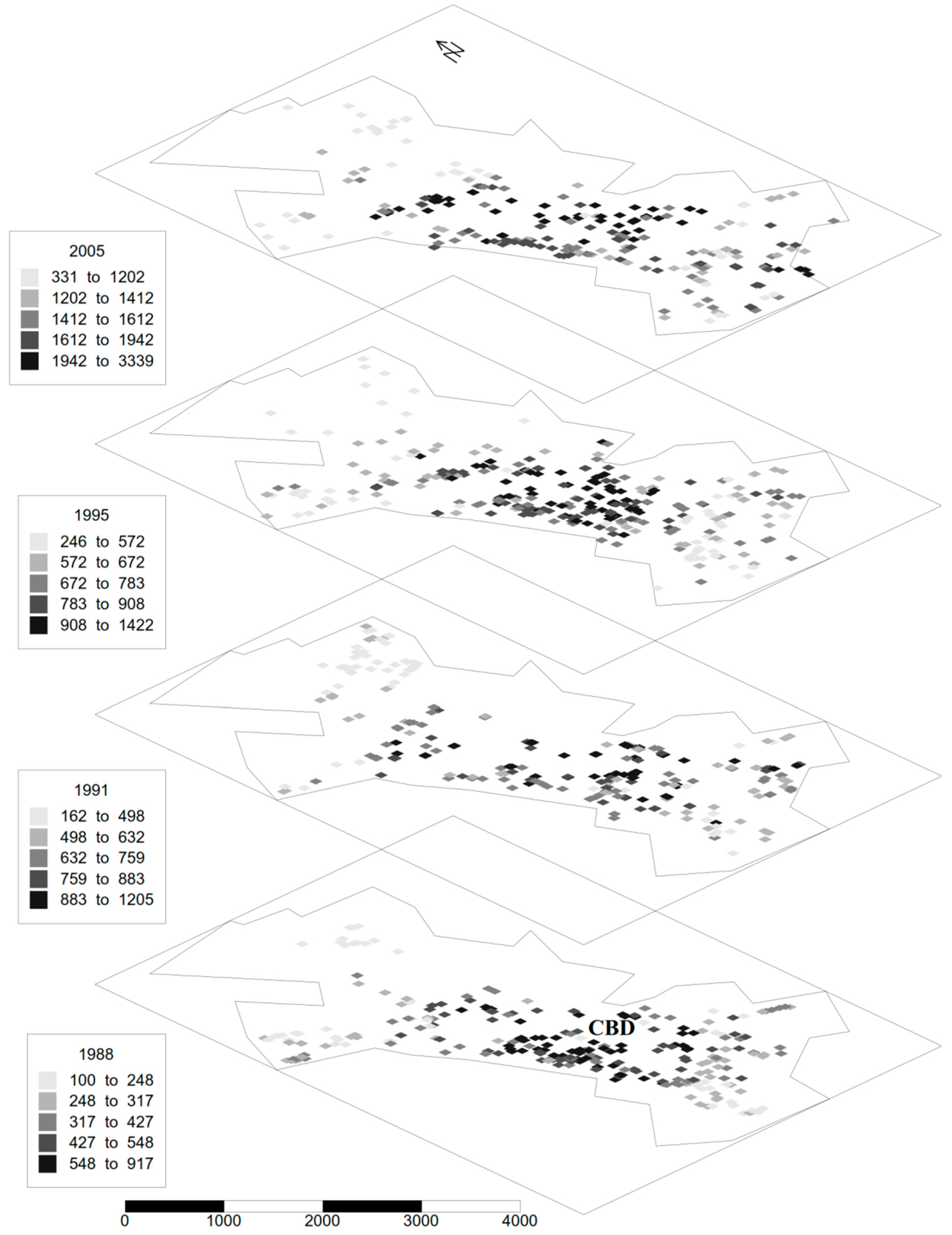
The city of Granada is elongated in shape (approximately 7000 m long by 2500 m wide), as it is bordered by a mountainous area to the east and a protected agricultural area to the west. As shown in Figure 3, the lowest-priced dwellings are located mainly in the northern part of the city. The geographical distribution of apartment prices reveals a convex behavior, since prices gradually fall when moving away from the central business district (CBD), where prices are the highest, to the outskirts of the city.
As occurs in most cities, housing prices in Granada are explained by a large number of variables, including structural attributes, neighborhood, and socioeconomic characteristics, and temporal variables. It is difficult to measure neighborhood and socioeconomic variables, as well as to identify the relevant neighborhood boundary [18,61]. The difficulty involved in measuring spatially different variables means that these variables are omitted in the hedonic prices equation, thus resulting in the spatial dependence of the error term, since the microlocation characteristics [62] have not been specified in the model. Different methods can be used to eliminate omitted variable bias due to missing spatial variables [4] from the standpoint of both geostatistics [30,63] and spatial econometrics using SEM [20,64,65].
In economics, it is common to use temporal deflators to try to regularize non-regular time series. However, the use of these temporal deflators, in addition to being artificial, involves a constant transformation for all the data in a given year, which does not affect the structure of direct or cross-autocorrelation. This is why the data have not been deflated to regularize the intervals, but raw data has been used. In the final results, the average annual rate of change for the periods is presented. This has allowed interpretation of the results despite the temporal irregularity of the data.
3.1. Database
In this study, we consider the classical specification of the hedonic housing price model, which distinguishes between two types of variables: structural variables and accessibility variables [8]. The structural variables are, for example, the age of the house, number of bathrooms, area, etc., and accessibility is frequently measured by the distance from the CBD. On the other hand, the error term includes the spatial dependence structure and the random component. In regard to the specification of the hedonic housing price model, it is very common to use a semilog model [66,67,68,69].
The list of the model variables and their definitions are provided below.
LPRICE: natural logarithm of apartment price in 1000 euros; it is the dependent variable.
AGE: age of apartment (in years) adjusted for major rehabilitation.
BATH: number of bathrooms in the apartment; this variable is considered an indicator of the quality of the apartment.
DIST: Euclidean distance in meters from the CBD. This represents the accessibility of the apartment at a large scale. In this paper, the distance from the CBD, which is one of the standard macrolocation characteristics [62], is assumed to be the main explanatory variable of the presence of large-scale patterns.
AREA: floor area of apartment in square meters.
FLOOR: binary variable that takes the value of 1 if the apartment is on a low floor.
ELEV: binary variable that takes the value of 1 if the building has an elevator.
HEAT: binary variable that takes the value of 1 if the apartment has central heating.
SPORT: binary variable that takes the value of 1 if the complex has sports facilities.
REHAB: binary variable that takes the value of 1 if the apartment must be remodeled.
The first four explanatory variables are included in all of the model equations, while the other variables are not present in all of them. The location of each dwelling is defined by its latitude and longitude coordinates in Universal Transverse Mercator (UTM) projection.
Table 1 provides the descriptive statistics of the variables. As can be seen in the table, the average price of the sample dwellings in the four years studied shows a similar growth to that observed in the city of Granada (Figure 2). The average number of bathrooms tends to increase, which can be interpreted as an increase in the quality of housing in that period. The mean of the variable AGE shows some growth, while the mean area of the dwellings is similar across years (between 109 and 118 m2). The mean distance to the CBD, in which the sample dwellings are located, ranges from 1300 to 1600 m in the different years. The floor area remains fairly stable at 108–119 m across the four years. The table shows the statistics for the distance between each dwelling and its nearest neighbor, which is less than 100 m on average in all years. Moreover, as can be observed in the table, information is not available for all the explanatory variables and years, thus indicating the heterogeneity of the data.
3.2. Results and Discussion
As indicated, given that not all the explanatory variables are available for every year, each model equation includes different explanatory variables. Thus, the multi-equation model is:
where the first equation corresponds to the year 2005, the second to 1995, the third to 1991, and the fourth to 1988.
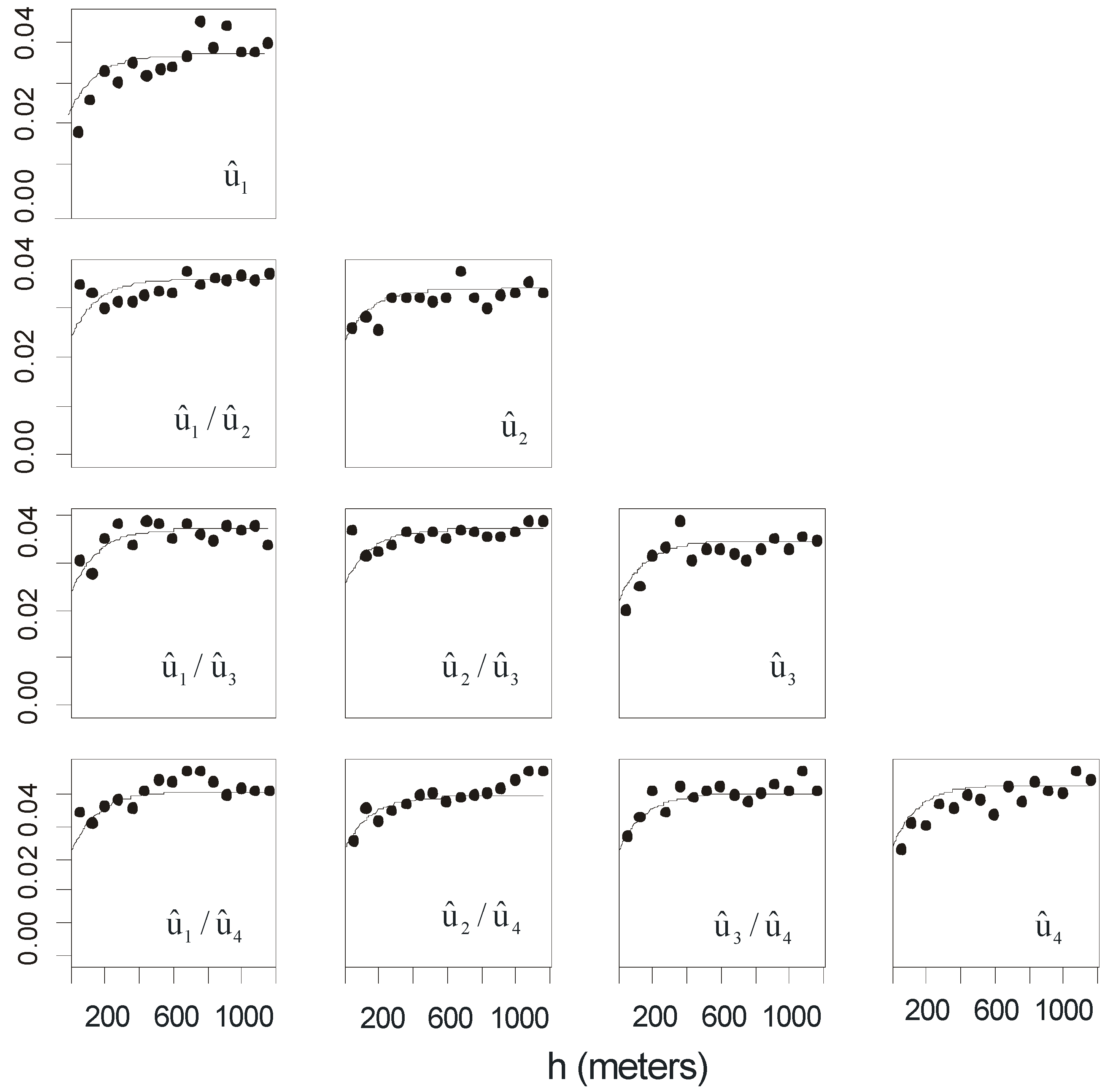
As mentioned above, the OLS estimator of the regression model parameters is inefficient when disturbances are spatially autocorrelated, whereas the GLS estimator is efficient. The spatial autocorrelation of the residuals was studied using the experimental variogram, while the coregionalization of the residuals was studied using the pseudo-cross-variogram [70]. Figure 4 shows the direct variograms (for each year) and the cross-variograms (between different years) of the residuals, all of which are observed to have a stationary shape. The prices might capture unobservable factors associated with the dwellings, thus resulting in the spatial autocorrelation of the residuals, which is reflected in the direct variograms. Moreover, homebuyers in the year 2005 may have known the selling prices of homes in previous years, and these prices can also be affected by unobservable factors. The cross-variograms capture the cross-correlation between these unobservable factors for each pair of years, hence the spatio-temporal relationship between them.
As the upward shape of the experimental variograms shows, the values of the residuals are not randomly distributed over the city map but spatially correlated and depend on the location of the dwellings. Thus, the degree of spatial correlation is higher (and the variogram value is lower) for units in close proximity (corresponding to low h values). For such units, overall housing tends to be similar. In contrast, the similarity in overall housing decreases as the distance separating the units increases, although this similarity tends to decrease with distance until becoming stable at around a range of 465 m (see Table 2). This distance includes the radius of influence at which the microlocation characteristics affect house prices. Although spatial autocorrelation has been observed, there is also a high degree of randomness. This randomness is reflected in the nugget values of the fitted variograms, which remain fairly stable over the four years. The exponential variogram model (Table 2) was fitted to each of the experimental variograms (see Figure 4). The method used to estimate the parameters of the variograms was implemented in FORTRAN using the LCMFIT2 program [71]. Anisotropy was not observed in any of the directional variograms for any year.
Several studies in both the natural and social sciences have fit an exponential variogram with cokriging [33,72,73]. In addition, a cross-validation was performed for each of the system equations with the three most common types of variogram models: the spherical, the exponential, and the Gaussian models (Table 3). In general, it can be observed that the exponential model provides the best results, as it has the highest R2cv and the lowest mean absolute error (MAE) and mean squared error (MSE) values.
The global drift multi-equation model () was estimated by GLS. The results of the estimation are presented in Table 4. In the estimated equations, all the variables are significant at a confidence level above or equal to 90%, with most being significant at 99%. All the signs of the coefficients are as expected (negative relation in the AGE, DIST, REHAB, and FLOOR variables, and a positive relation in the rest of the variables).
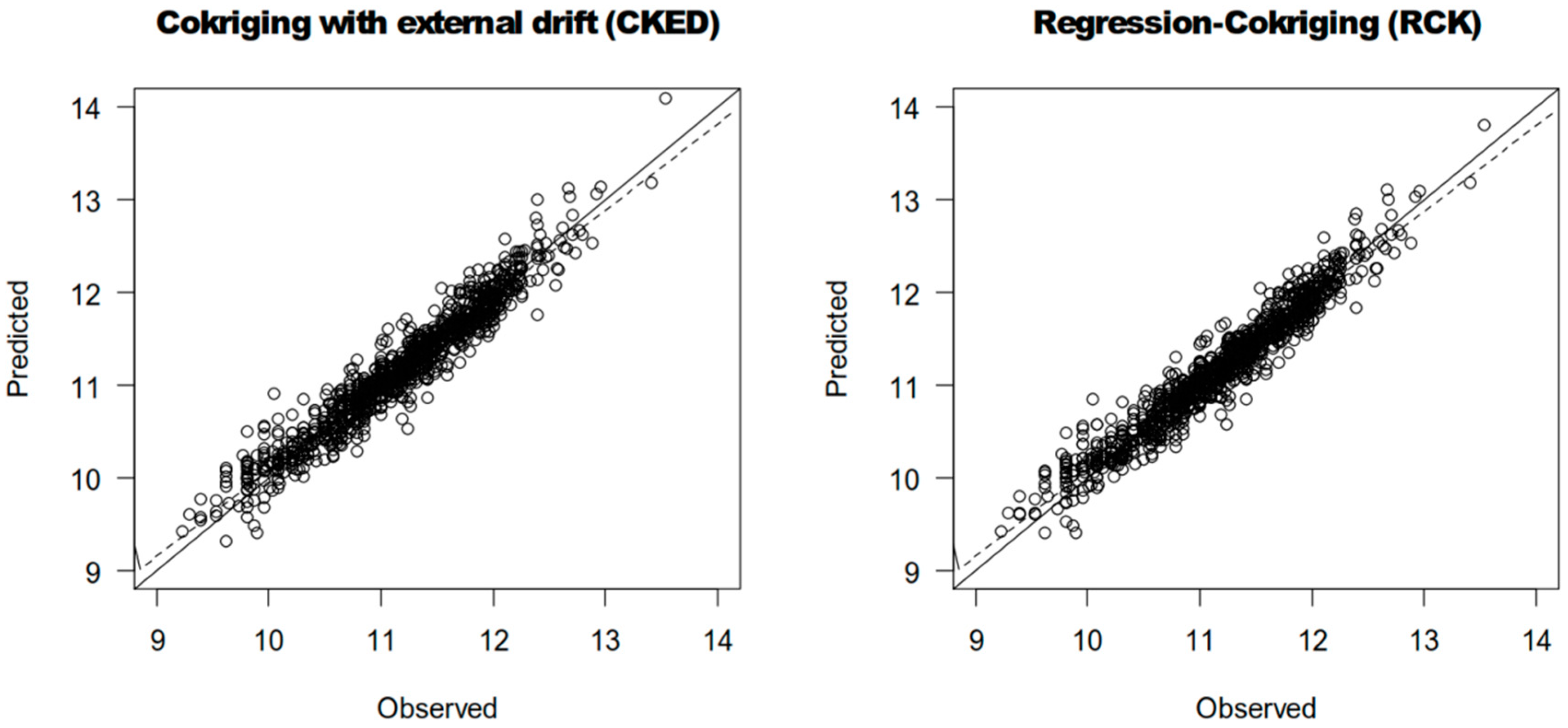
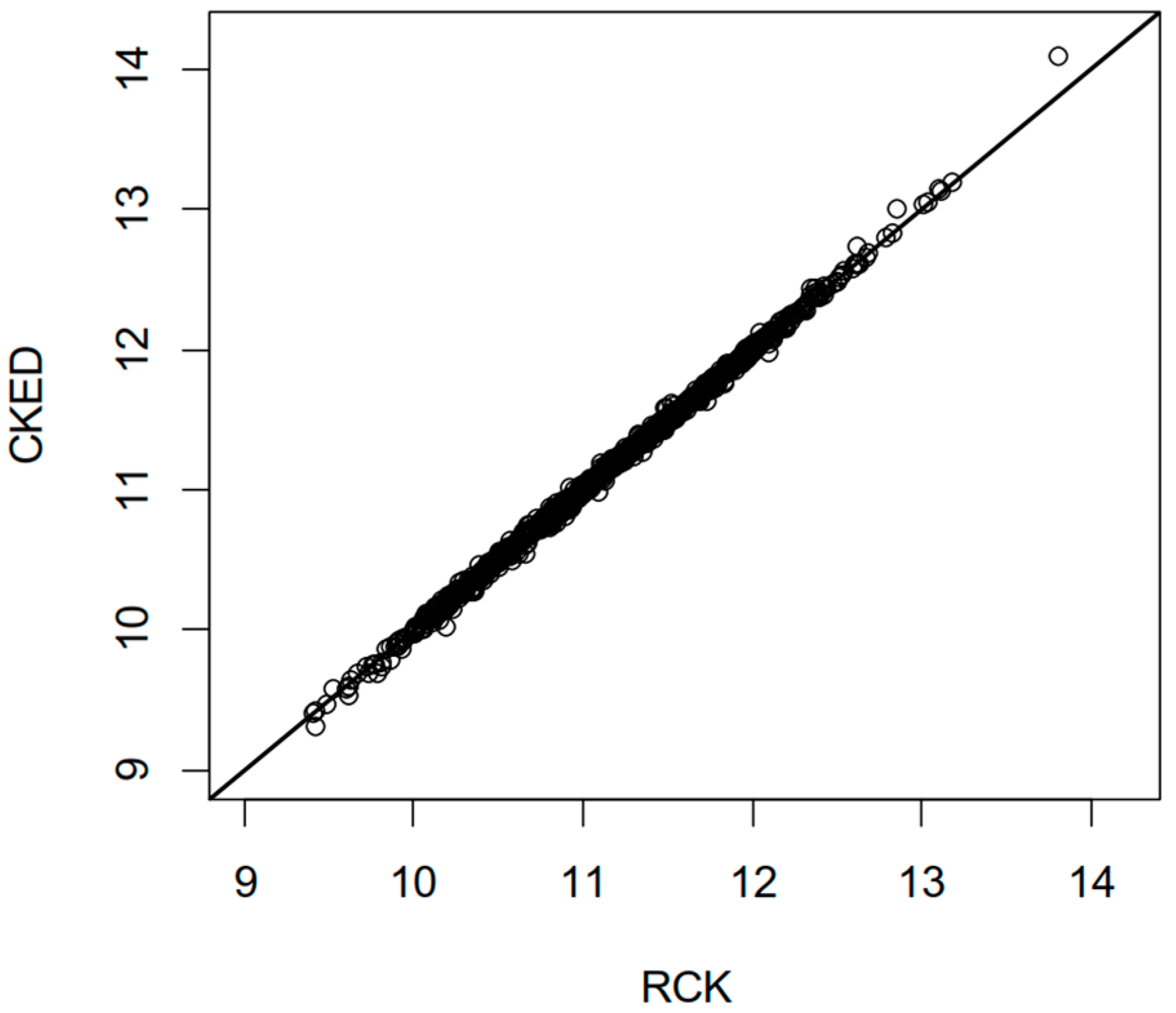
In this paper, the CKED and RCK methods are applied. In order to compare both methods, a cross-validation method has been used, specifically leave-one-out cross-validation (LOOCV). LOOCV allows for comparison of predicted and observed values using only the information available in the sample dataset. The LOOCV procedure consists of temporarily discarding a sample value at a particular location from the sample data set, and then estimating the value at the same location using the remaining samples [55]. This procedure is repeated for all the experimental points in order to compare the observed values to the predicted values using statistical and visual tools. The cross-validation statistics used are mean absolute error (MAE), mean squared error (MSE), and R-squared of cross-validation, which is obtained from the square of the correlation between the model’s predicted values and the observed values (). As can be seen in Table 5, the two methods show similar cross-validation statistics, although those of the RCK method are slightly better, as the value is closer to one and the other statistics are closer to zero. Figure 5 shows the regression between the predicted and observed data with RCK and CKED. As can be observed, the two scatterplots are quite similar and the regression line is very close to the 1:1 line. Moreover, Figure 6 shows the RCK versus the CKED predictions. As can be seen, the predictions obtained with both methods are very similar.
Additionally, in order to compare the predictions of traditional OLS and cokriging, Table 6 shows the OLS estimates for each of the equations. This permits quantification of the added value of the cokriging method versus OLS. As can be observed in the table, all the variables are significant, as was the case with RCK.
This study has considered accessibility to the CBD, which is one of the main locational variables. However, other relevant variables have been omitted (i.e., provision of public and private services, socio-economic and environmental variables, etc.). Therefore, the differences observed between the OLS coefficients (see Table 6) and RCK (see Table 4) may be due to this omission. It is difficult to specify these locational factors and quantify their radius of influence, since they usually refer to areas whose sizes and shapes tend to be subjective [30,74]. In fact, numerous studies on hedonic models have mostly included structural variables and omitted relevant characteristics of the location [8,9,31,43,75]. Nevertheless, models that correct this omission by considering the presence of spatial autocorrelation in disturbances, such as the SEM and RCK models, provide better results than OLS [4]. Therefore, an advantage of the RCK model is that it improves the estimates by indirectly considering the omission of relevant variables through modeling the correlation between disturbances.
Table 6 shows the results of the cross-validation. It is important to keep in mind that in traditional OLS, all observations are used to fit the model, while this does not occur in cross-validation. Since the R-squared of the OLS model is not directly comparable to the of the RCK model, the and other statistics for the OLS models have been obtained using cross-validation (MAE and MSE). Table 7 shows the improvement in % by RCK over OLS. Specifically, the in the RCK model shows an almost 8% improvement over OLS, while the MAE shows an improvement of approximately 18% and the MSE of more than 30%. As can be seen, there is a clear improvement in the predictive ability of the RCK model, thus supporting the added value of the spatial effect and the cross between space and time.
The co-dispersion coefficients have also been obtained. These coefficients provide an interpretive tool to analyze the correlation between the variation between two dates [76]:
If coefficients are constant, the correlation of the variable in two dates does not depend on the spatial scale, which is referred to as intrinsic correlation [52]. However, if the correlation is affected by spatial scale () are not constant), it is necessary to cokrige the variable, as suggested by the right-hand path [70]. The experimental co-dispersion function () is represented in Figure 7 and shows the correlation coefficients between two dates by h-increments. Since a constant function behavior is not observed, it is appropriate to use cokriging.
3.3. Estimation of Spatial Price Variation in Multi-Years
From the standpoint of the housing market, it is clearly of interest to determine spatio-temporal variation in housing prices [24,77] at any location, and thus obtain flat isovalue maps of these changes [18,78]. To do so, it is necessary to first estimate the price of housing for each of the years observed at any point on the map. Since it is not possible to know the explanatory characteristics at each point of the map, with the exception of the variable DIST (which was calculated for each point to be estimated), a standard dwelling on which to make the prediction must be defined. A standard dwelling is obtained by assigning the numerical value of the sample average of these characteristics to each of the structural characteristics of the dwelling. Because the model estimates show the estimated value of a standard dwelling in different locations in space, the spatial distribution of the prices estimated with the proposed model are caused by the value of the location. In this work, a standard dwelling is defined according to the following values:
AGE = 16, AREA = 113, BATH = 1, FLOOR = 0, ELEV = 1, HEAT = 1, SPORT = 0, and REHAB = 0.
The values for the standard dwelling variables are the arithmetic means of AGE and AREA, while the mode has been used for the rest of the variables.
Therefore, the procedure to obtain the spatio-temporal variation was as follows. First, using each of the methods, spatial estimates were performed to obtain the price of a standard dwelling at the nodes of a mesh inserted in the city map, which forms square cells measuring 100 meters per side. Once the prices were estimated at the mesh nodes for each year, the average annual rate of change (AARC) in prices was calculated for each period. The AARC was calculated using the following expression:
where and are the prices of a standard dwelling estimated in the final and initial year of the period, respectively; and n is the length, in years, of the period.
The AARC is 26% for the period 1988–1991, 3% for the period 1991–1995, and 8% for the period 1995–2005. For these same periods, the AARC obtained from data published by the Sociedad de Tasación, which uses sample dwellings that differ from those of this study, are 21%, 4%, and 9%, respectively.
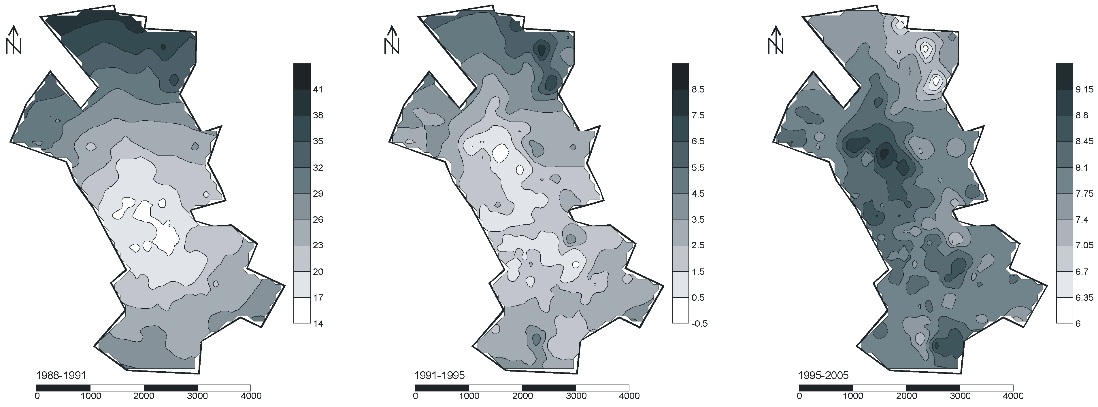
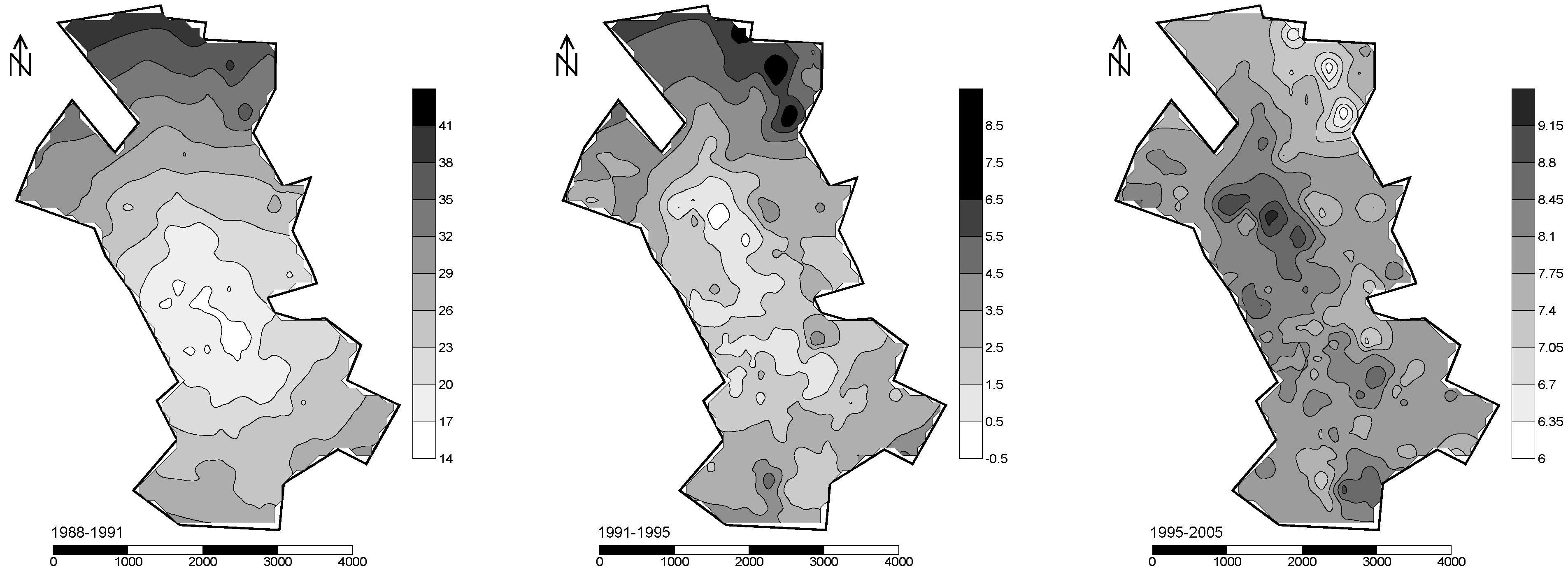
Finally, these variations are used to obtain the AARC isovalue maps for the three periods by means of RCK (see Figure 8) and CKED (see Figure 9). The results obtained by both methods are very similar. It should be noted that in the first period (1988–1991), the AARC spatial range of variation (14% to 44%) is much higher than in the period 1991–1995 (−0.5% to 9%) and the period 1995–2005 (6% to 9.5%). This indicates a high degree of spatial heterogeneity in price variation in the first period, while there is less spatial heterogeneity in the third period. These maps show how the price variation of standard dwellings is spatially distributed. Thus, in the first period, the explanatory variable distance to city center (DIST) has the strongest effect, and produces a U effect in the variations. Furthermore, the largest increases occur in the outskirts, particularly in the northern third part of the city, which is where the lowest prices (see Figure 3) are located. These marked increases are due to the extensive urban development and greater provision of services in this area. In the period 1991–1995, the increases are again higher in the outskirts of the city, although they are more moderate than in the previous period due to the stabilization of urban development at this time. Moreover, price variation is generally observed to have a more irregular distribution than in the preceding period. Thus, in the first period, a clear U-shaped behavior with low values in the center can be observed, which steadily increases towards the periphery. However, the variations are more irregular in the second period. Finally, in the last period, the observed behavior is opposite to that of prior periods, since the largest increases occur in the central third part of the city, largely due to the rehabilitation of housing, while the smallest increases are observed in the northern part. In addition, the variable DIST is not observed to have such a dominant effect in the last two periods.
In using a standard dwelling to make these estimates, what stands out most in these estimated prices is their location, thus indicating that the price variation obtained with these methods in different parts of the map is attributable to the different spatial characteristics (macro and microlocation characteristics). This is consistent with the theory that structural characteristics are theoretically reproducible anywhere on the map, but not spatial characteristics [79,80].
4. Discussions and Conclusions
Given the importance of understanding spatio-temporal variation in housing prices in the real estate market and obtaining isovalue maps of these variations, a method to develop these maps has been presented.
Since heterotopic data have been used, it has not been possible to determine the true price variation for the same dwelling at two points in time. With the proposed method, however, it is possible to estimate spatio-temporal variation in housing prices with heterotopic samples, which is undoubtedly one of the main contributions of this work. In addition, this method enables management of the heterogeneity of both the data and the explanatory variables observed in the different years. This procedure is based on a multi-equation hedonic regression model with spatial autocorrelation and temporal cross-correlation in the disturbances.
In this paper, an application of this procedure to predict spatio-temporal variation in housing prices for the city of Granada has been presented. In the first two periods (1988–1991 and 1991–1995), the largest variations occur in the city outskirts, while in the last period (1995–2005), the largest variations were observed in the central third part of the city. The increases observed in the first two periods are due to urban development and the provision of services in the northern area. In the third period, however, the increase observed in the central third part of the city is the result of housing rehabilitation.
Finally, it is important to highlight that the proposed procedure to obtain the spatio-temporal variation can be implemented with the CKED and RCK methods. In comparing the two methods, the main conclusion is that in our case, the cross-validation results are similar, although slightly better for RCK. While RCK is more cumbersome than CKED, the first method is more versatile as it can be easily combined with any generalized additive model.
This work could be improved by including socio-economic neighborhood characteristics in the model, since it would allow quantification of the effect of these factors on the spatio-temporal variation in housing prices.
Author Contributions
Conceptualization, software, validation, resources, data curation, writing—original draft preparation, writing—review and editing, supervision, project administration and funding acquisition, J.C.-O. and R.C.-G.; methodology, formal analysis, visualization and investigation, J.C.-O., R.C.-G. and M.C.-R..
Funding
This work was conducted within the framework of a research project granted by CEMIX-6/16 and financed by Banco Santander.
Acknowledgments
We are also grateful to Colonel Ángel F. Blázquez Diéguez of the Spanish Army for mentoring this research project.
Conflicts of Interest
The authors declare no conflicts of interest.
References
- Anselin, L. Thirty years of spatial econometrics. Reg. Sci. 2010, 89, 3–25. [Google Scholar] [CrossRef]
- Bourassa, S.C.; Cantoni, E.; Hoesli, M. Predicting House Prices with Spatial Dependence: A Comparison of Alternative Methods. J. Hous. Res. 2010, 32, 139–159. [Google Scholar]
- Páez, A. Recent research in spatial real estate hedonic analysis. J. Geogr. Syst. 2009, 11, 311–316. [Google Scholar] [CrossRef] [Green Version]
- Krause, A.; Bitter, C. Spatial econometrics, land values and sustainability: Trends in real estate valuation research. Cities 2012, 29, S19–S25. [Google Scholar] [CrossRef]
- Del Giudice, V.; De Paola, P.; Forte, F.; Manganelli, B. Real Estate Appraisals with Bayesian Approach and Markov Chain Hybrid Monte Carlo Method: An Application to a Central Urban Area of Naples. Sustainability 2017, 9, 2138. [Google Scholar] [CrossRef]
- Rosen, S. Hedonic Prices and Implicit Markets: Product Differentiation in Pure Com-petition. J. Political Econ. 1974, 82, 34–55. [Google Scholar] [CrossRef]
- Anselin, L. Spatial Econometrics: Methods and Models; Kluwer Academic Publishers: Dordrecht, The Netherlands, 1988. [Google Scholar]
- Can, A. Specification and estimation of hedonic housing price models. Reg. Sci. Urban Econ. 1992, 22, 453–474. [Google Scholar] [CrossRef]
- Dubin, R.A. Spatial autocorrelation and neighborhood quality. Reg. Sci. Urban Econ. 1992, 22, 433–452. [Google Scholar] [CrossRef]
- Militino, A.F.; Ugarte, M.D.; Garcia-Reinaldos, L. Alternative models for describing spatial dependence among dwelling selling prices. J. Real Estate Financ. Econ. 2004, 29, 193–209. [Google Scholar] [CrossRef]
- Cressie, N. Statistics for Spatial Data; John Wiley & Sons: Hoboken, NJ, USA, 1991. [Google Scholar]
- Tsutsumi, M.; Seya, H. Measuring the impact of large-scale transportation projects on land price using spatial statistical models. Pap. Reg. Sci. 2008, 87, 385–401. [Google Scholar] [CrossRef]
- de Koning, K.; Filatova, T.; Bin, O. Improved Methods for Predicting Property Prices in Hazard Prone Dynamic Markets. Environ. Resour. Econ. 2018, 69, 247–263. [Google Scholar] [CrossRef]
- Hoshino, T.; Kuriyama, K. Measuring the benefits of neighbourhood park amenities: Application and comparison of spatial hedonic approaches. Environ. Resour. Econ. 2010, 45, 429–444. [Google Scholar] [CrossRef]
- Osland, L.; Thorsen, I. Effects on housing prices of urban attraction and labor-market accessibility. Environ. Plan. A 2008, 40, 2490. [Google Scholar] [CrossRef]
- Trojanek, R.; Gluszak, M. Spatial and time effect of subway on property prices. J. Hous. Built Environ. 2018, 33, 359–384. [Google Scholar] [CrossRef]
- Pace, R.K.; Barry, R.; Clapp, J.M.; Rodriquez, M. Spatiotemporal autoregressive models of neighborhood effects. J. Real Estate Financ. Econ. 1998, 17, 15–33. [Google Scholar] [CrossRef]
- Clapp, J.M. A Semiparametric Method for Estimating Local House Price Indices. Real Estate Econ. 2004, 32, 127–160. [Google Scholar] [CrossRef]
- Sun, H.; Tu, Y.; Yu, S.-M. A Spatio-Temporal Autoregressive Model for Multi-Unit Residential Market Analysis. J. Real Estate Financ. Econ. 2005, 31, 155–187. [Google Scholar] [CrossRef]
- Pace, R.; Barry, R.; Gilley, O.W.; Sirmans, C.F. A method for spatial-temporal forecasting with an application to real estate prices. Int. J. Forecast. 2000, 16, 229–246. [Google Scholar] [CrossRef]
- Dubin, R.A.; Pace, J.K.; Thibodeau, T.G. Spatial Autoregression Techniques for Real Estate Data. J. Real Estate Lit. 1999, 7, 79–95. [Google Scholar] [CrossRef]
- McGreal, S.; Taltavull de La Paz, P. Implicit House Prices: Variation over Time and Space in Spain. Urban Stud. 2013, 50, 2024–2043. [Google Scholar] [CrossRef]
- Beamonte San Agustín, A.; Gargallo Valero, P.; Figueras Salvador, M. Evolución espacio-temporal del mercado inmobiliario en Zaragoza mediante el uso de efectos de vecindad. Estadística Española 2008, 50, 5–24. [Google Scholar]
- Huang, B.; Wu, B.; Barry, M. Geographically and temporally weighted regression for modeling spatio-temporal variation in house prices. Int. J. Geogr. Inf. Sci. 2010, 24, 383–401. [Google Scholar] [CrossRef]
- Wu, B.; Li, R.; Huang, B. A geographically and temporally weighted autoregressive model with application to housing prices. Int. J. Geogr. Inf. Sci. 2014, 28, 1186–1204. [Google Scholar] [CrossRef]
- Yao, J.; Stewart Fotheringham, A. Local Spatiotemporal Modeling of House Prices: A Mixed Model Approach. Prof. Geogr. 2016, 68, 189–201. [Google Scholar] [CrossRef]
- Helbich, M.; Griffith, D.A. Spatially varying coefficient models in real estate: Eigenvector spatial filtering and alternative approaches. Comput. Environ. Urban Syst. 2016, 57, 1–11. [Google Scholar] [CrossRef]
- Montero-Lorenzo, J.; Larraz-Iribas, B. Space-time approach to commercial property prices valuation. Appl. Econ. 2012, 44, 3705–3715. [Google Scholar] [CrossRef] [Green Version]
- Chica-Olmo, J. Prediction of Housing Location Price by a Multivariate Spatial Method: Cokriging. J. Real Estate Res. 2007, 29, 91–114. [Google Scholar]
- Chica-Olmo, J.; Cano-Guervos, R.; Chica-Olmo, M. A Coregionalized Model to Predict Housing Prices. Urban Geogr. 2013, 34, 395–412. [Google Scholar] [CrossRef]
- Kuntz, M.; Helbich, M. Geostatistical mapping of real estate prices: An empirical comparison of kriging and cokriging. Int. J. Geogr. Inf. Sci. 2014, 28, 1904–1921. [Google Scholar] [CrossRef]
- D’Agostino, V.; Greene, E.A.; Passarella, G.; Vurro, M. Spatial and temporal study of nitrate concentration in groundwater by means of coregionalization. Environ. Geol. 1998, 36, 285–295. [Google Scholar] [CrossRef]
- Fassò, A.; Finazzi, F. Maximum likelihood estimation of the dynamic coregionalization model with heterotopic data. Environmetrics 2011, 22, 735–748. [Google Scholar] [CrossRef]
- Joyner, T.A.; Friedland, C.J.; Rohli, R.V.; Treviño, A.M.; Massarra, C.; Paulus, G. Cross-correlation modeling of European windstorms: A cokriging approach for optimizing surface wind estimates. Spat. Stat. 2015, 13, 62–75. [Google Scholar] [CrossRef]
- Lark, R. Robust estimation of the pseudo cross-variogram for cokriging soil properties. Eur. J. Soil Sci. 2002, 53, 253–270. [Google Scholar] [CrossRef]
- Gallois, D.; de Fouquet, C.; Le Loc’h, G.; Malherbe, L.; Cardenas, G. Mapping Annual Nitrogen Dioxide Concentrations in Urban Areas. In Geostatistics Banff 2004; Springer: Berlin, Germany, 2005; pp. 1087–1096. [Google Scholar]
- Kyriakidis, P.C.; Journel, A.G. Geostatistical Space Time Models: A Review. Math. Geol. 1999, 31, 651–684. [Google Scholar] [CrossRef]
- De Iaco, S.; Myers, D.E.; Posa, D. Space-time variograms and a functional form for total 3 air pollution measurements. Comput. Stat. Data Anal. 2002, 41, 311–328. [Google Scholar] [CrossRef]
- Schabenberger, O.; Gotway, C.A. Statistical Methods for Spatial Data Analysis; Chapman & Hall/CRC Press: Boca Raton, FL, USA, 2005. [Google Scholar]
- Montero, J.-M.; Fernández-Avilés, G.; Mateu, J. Spatial and Spatio-Temporal Geostatistical Modeling and Kriging; John Wiley & Sons: Hoboken, NJ, USA, 2015. [Google Scholar]
- Li, L.; Revesz, P. Interpolation methods for spatio-temporal geographic data. Comput. Environ. Urban Syst. 2004, 28, 201–227. [Google Scholar] [CrossRef]
- Papritz, A.; Flühler, H. Temporal change of spatially autocorrelated soil properties: Optimal estimation by cokriging. Geoderma 1994, 62, 29–43. [Google Scholar] [CrossRef]
- Gelfand, A.E.; Ecker, M.D.; Knight, J.R.; Sirmans, C.F. The Dynamics of Location in Home Price. J. Real Estate Financ. Econ. 2004, 29, 149–166. [Google Scholar] [CrossRef]
- Myers, D.E. Matrix Formulation of Cokriging. Math. Geol. 1982, 14, 249–257. [Google Scholar] [CrossRef]
- Ver Hoef, J.M.; Cressie, N. Multivariable Spatial Prediction. Math. Geol. 1993, 25, 219–240. [Google Scholar] [CrossRef]
- Neuman, S.P.; Jacobson, E.A. Analysis of non-intrinsic spatial variability by residual kriging with application to regional groundwater levels. Math. Geol. 1984, 16, 499–521. [Google Scholar] [CrossRef]
- Militino, A.; Palacios, M.; Ugarte, M. Robust predictions of rainfall in Navarre, Spain. In geoENV III—Geostatistics for Environmental Applications; Springer: Berlin, Germany, 2001; pp. 79–90. [Google Scholar]
- Pebesma, E.J. Multivariable geostatistics in S: The gstat package. Comput. Geosci. 2004, 30, 683–691. [Google Scholar] [CrossRef]
- Hengl, T.; Heuvelink, G.; Stein, A. Comparison of Kriging with External Drift and Regression-Kriging; Technical Note; ITC: Enschede, The Netherlands, 2003.
- McBratney, A.B.; Odeh, I.O.; Bishop, T.F.; Dunbar, M.S.; Shatar, T.M. An overview of pedometric techniques for use in soil survey. Geoderma 2000, 97, 293–327. [Google Scholar] [CrossRef]
- Hengl, T.; Heuvelink, G.; Rossiter, D.G. About regression-kriging: From equations to case studies. Comput. Geosci. 2007, 33, 1301–1315. [Google Scholar] [CrossRef]
- Matheron, G. Les Variables Regionalisées et Leur Estimation; Masson y Cie: Paris, France, 1965. [Google Scholar]
- Myers, D.E. Pseudo-Cross Variograms, Positive-Definiteness, and Cokriging. Math. Geol. 1991, 23, 805–816. [Google Scholar] [CrossRef]
- Journel, A.G.; Huijbregts, C.J. Mining Geostatistics; Academic Press: London, UK, 1978. [Google Scholar]
- Isaaks, E.H.; Srivastava, R.M. An Introduction to Applied Geostatistics; Oxford University Press: New York, NY, USA, 1989. [Google Scholar]
- Goulard, M.; Voltz, M. Linear coregionalization model: Tools for estimation and choice of cross-variogram matrix. Math. Geol. 1992, 24, 269–286. [Google Scholar] [CrossRef] [Green Version]
- Goetzmann, W.N.; Spiegel, M. A spatial model of housing returns and neighborhood substitutability. J. Real Estate Financ. Econ. 1997, 14, 11–31. [Google Scholar] [CrossRef]
- Hwang, M.; Quigley, J.M. Economic fundamentals in local housing markets: Evidence from US metropolitan regions. J. Reg. Sci. 2006, 46, 425–453. [Google Scholar] [CrossRef]
- Quercia, R.G.; McCarthy, G.W.; Ryznar, R.M.; Can Talen, A. Spatio-Temporal Measurement of House Price Appreciation in Underserved Areas. J. Hous. Res. 2000, 11, 1–28. [Google Scholar]
- Kuethe, T.H.; Pede, V.O. Regional housing price cycles: A spatio-temporal analysis using US state-level data. Reg. Stud. 2011, 45, 563–574. [Google Scholar] [CrossRef]
- Arribas, I.; García, F.; Guijarro, F.; Oliver, J.; Tamošiūnienė, R. Mass appraisal of residential real estate using multilevel modelling. Int. J. Strateg. Prop. Manag. 2016, 20, 77–87. [Google Scholar] [CrossRef]
- Derycke, P.-H. Economie et Planification Urbaines: L’espace Urbain; Presses Universitaires de France: Paris, France, 1979; Volume 1. [Google Scholar]
- Yoo, E.-H.; Kyriakidis, P.C. Area-to-point Kriging in spatial hedonic pricing models. J. Geogr. Syst. 2009, 11, 381–406. [Google Scholar] [CrossRef]
- Brasington, D.M.; Haining, R. Parents, peers, or school inputs: Which components of school outcomes are capitalized into house value? Reg. Sci. Urban Econ. 2009, 39, 523–529. [Google Scholar] [CrossRef]
- Lacombe, D.J.; LeSage, J.P. Using Bayesian posterior model probabilities to identify omitted variables in spatial regression models. Pap. Reg. Sci. 2015, 94, 365–383. [Google Scholar] [CrossRef]
- Mueller, J.M.; Loomis, J.B. Spatial dependence in hedonic property models: Do different corrections for spatial dependence result in economically significant differences in estimated implicit prices? J. Agric. Resour. Econ. 2008, 33, 212–231. [Google Scholar]
- Chica-Olmo, J. Spatial Estimation of Housing Prices and Locational Rents. Urban Stud. 1995, 32, 1331–1344. [Google Scholar] [CrossRef]
- Brunauer, W.; Lang, S.; Umlauf, N. Modelling house prices using multilevel structured additive regression. Stat. Model. 2013, 13, 95–123. [Google Scholar] [CrossRef]
- Seo, D.; Chung, Y.; Kwon, Y. Price determinants of affordable apartments in Vietnam: Toward the public–private partnerships for sustainable housing development. Sustainability 2018, 10, 197. [Google Scholar] [CrossRef]
- Wackernagel, H. Multivariate Geostatistics; Springer: Berlin, Germany, 1995. [Google Scholar]
- Pardo-Igúzquiza, E.; Dowd, P.A. FACTOR2D: A computer program for factorial cokriging. Comput. Geosci. 2002, 28, 857–875. [Google Scholar] [CrossRef]
- Li, Z.; Zhang, Y.-K.; Schilling, K.; Skopec, M. Cokriging estimation of daily suspended sediment loads. J. Hydrol. 2006, 327, 389–398. [Google Scholar] [CrossRef]
- Wu, C.; Murray, A.T. A cokriging method for estimating population density in urban areas. Comput. Environ. Urban Syst. 2005, 29, 558–579. [Google Scholar] [CrossRef]
- Dubin, R.A. Spatial Autocorrelation: A Primer. J. Hous. Econ. 1998, 7, 304–327. [Google Scholar] [CrossRef]
- Liu, X. Spatial and temporal dependence in house price prediction. J. Real Estate Financ. Econ. 2013, 47, 341–369. [Google Scholar] [CrossRef]
- Bourennane, H.; Nicoullaud, B.; Couturier, A.; Mary, B.; Richard, G.; King, D.; Stafford, J. A Potential Role of Permanent Soil Variables and Field Topography to Reveal Scale Dependence and the Temporal Persistence of Soil Water Content Spatial Patterns. In Proceedings of the Precision Agriculture’05, 5th European Conference on Precision Agriculture, Uppsala, Sweden, 2005; Wageningen Academic Publishers: Wageningen, The Netherlands, 2005; pp. 769–777. [Google Scholar]
- Le Goix, R.; Vesselinov, E. Gated communities and house prices: Suburban change in southern California, 1980–2008. Int. J. Urban Reg. Res. 2013, 37, 2129–2151. [Google Scholar] [CrossRef]
- Yue, W.; Liu, Y.; Fan, P. Polycentric urban development: The case of Hangzhou. Environ. Plan. A 2010, 42, 563. [Google Scholar] [CrossRef]
- Kiel, K.A.; Zabel, J.E. Location, location, location: The 3L Approach to house price determination. J. Hous. Econ. 2008, 17, 175–190. [Google Scholar] [CrossRef]
- Cheshire, P.; Sheppard, S. On the price of land and the value of amenities. Economica 1995, 62, 247–267. [Google Scholar] [CrossRef]
Figure 1.
Location of the study area.

Figure 2.
Housing prices from 1987 to 2005 for Spain, Andalusia, and Granada (standard dwelling of 100m2). Source: Sociedad de Tasación.
Figure 2.
Housing prices from 1987 to 2005 for Spain, Andalusia, and Granada (standard dwelling of 100m2). Source: Sociedad de Tasación.

Figure 3.
Housing prices (€/m2) in 1988, 1991, 1995, and 2005 in Granada.

Figure 4.
Experimental variograms and fitted models of the residuals () of the multi-equation model. Note: Direct variograms: (2005) to (1988); and cross-variograms: , , etc.
Figure 4.
Experimental variograms and fitted models of the residuals () of the multi-equation model. Note: Direct variograms: (2005) to (1988); and cross-variograms: , , etc.

Figure 5.
Regression between predicted and observed data. Note: The solid straight line represents the 1:1 line and the dashed line represents the regression line.
Figure 5.
Regression between predicted and observed data. Note: The solid straight line represents the 1:1 line and the dashed line represents the regression line.

Figure 6.
Comparison of RCK and CKED predictions.

Figure 7.
Co-dispersion coefficients between different years.

Figure 8.
Average annual rate of change in housing prices in the three periods with RCK.

Figure 9.
Average annual rate of change in housing prices in the three periods with CKED.


Table 1.
Descriptive statistics of the variables of samples (PRICE in 1000 euros) and nearest neighbor statistics of distance (Nearest, in meters).
Table 1.
Descriptive statistics of the variables of samples (PRICE in 1000 euros) and nearest neighbor statistics of distance (Nearest, in meters).
| Minimum | Maximum | Mean | Standard Deviation | |||||||||||||
|---|---|---|---|---|---|---|---|---|---|---|---|---|---|---|---|---|
| 1988 | 1991 | 1995 | 2005 | 1988 | 1991 | 1995 | 2005 | 1988 | 1991 | 1995 | 2005 | 1988 | 1991 | 1995 | 2005 | |
| PRICE | 10.22 | 15.03 | 15.03 | 22.83 | 240.407 | 300.51 | 330.55 | 751.26 | 45.89 | 75.56 | 90.51 | 162.40 | 30.60 | 36.65 | 50.03 | 85.55 |
| AGE | 1 | 1 | 1 | 2 | 40 | 81 | 84 | 40 | 13.58 | 11.51 | 16.96 | 23.44 | 7.56 | 9.72 | 11.69 | 8.93 |
| BATH | 1 | 1 | 1 | 1 | 3 | 3 | 3 | 4 | 1.23 | 1.51 | 1.60 | 1.45 | 0.44 | 0.56 | 0.54 | 0.58 |
| DIST | 166.30 | 294.98 | 76.39 | 81.27 | 3511.29 | 3723.63 | 3695.92 | 3940.96 | 1492.94 | 1577.95 | 1326.28 | 1557.46 | 851.91 | 963.64 | 812.76 | 823.68 |
| AREA | 65.00 | 49.00 | 40.00 | 40.00 | 340.00 | 320.00 | 325.00 | 390.00 | 109.86 | 112.85 | 118.13 | 108.80 | 33.00 | 35.27 | 42.48 | 38.64 |
| FLOOR | - | - | - | 0 | - | - | - | 1 | - | - | - | 0.039 | - | - | - | 0.19 |
| ELEV | - | - | 0 | 0 | - | - | 1 | 1 | - | - | 0.88 | 0.78 | - | - | 0.31 | 0.41 |
| HEAT | - | - | 0 | 0 | - | - | 1 | 1 | - | - | 0.55 | 0.54 | - | - | 0.50 | 0.50 |
| SPORT | - | - | - | 0 | - | - | - | 1 | - | - | - | 0.06 | - | - | - | 0.24 |
| REHAB | - | - | - | 0 | - | - | - | 1 | - | - | - | 0.35 | - | - | - | 0.48 |
| Nearest | 8.10 | 10.34 | 6.00 | 4.20 | 390.77 | 385.38 | 666.40 | 646.87 | 74.67 | 55.75 | 86.81 | 98.22 | 55.45 | 63.06 | 88.60 | 100.24 |
Table 2.
Parameters of fitted direct variograms and cross-variograms of residuals from the multi-equation model.
Table 2.
Parameters of fitted direct variograms and cross-variograms of residuals from the multi-equation model.
| Residuals | Nugget | Partial Sill | Practical Range |
|---|---|---|---|
| (2005) | 0.023 | 0.015 | 465.00 |
| (1995) | 0.025 | 0.011 | 465.00 |
| (1991) | 0.026 | 0.014 | 465.00 |
| (1988) | 0.044 | 0.024 | 465.00 |
| 0.024 | 0.012 | 465.00 | |
| 0.024 | 0.014 | 465.00 | |
| 0.032 | 0.019 | 465.00 | |
| 0.025 | 0.011 | 465.00 | |
| 0.034 | 0.016 | 465.00 | |
| 0.033 | 0.018 | 465.00 |
Table 3.
Cross-validation for different variogram models.
| R2cv | MAE | MSE | |
|---|---|---|---|
| 1988 | |||
| Spherical | 0.8349 | 0.1862 | 0.0557 |
| Gaussian | 0.8461 | 0.1806 | 0.0519 |
| Exponential | 0.8507 | 0.1793 | 0.0503 |
| 1991 | |||
| Spherical | 0.8639 | 0.1406 | 0.0340 |
| Gaussian | 0.8719 | 0.1356 | 0.0320 |
| Exponential | 0.8727 | 0.1371 | 0.0318 |
| 1995 | |||
| Spherical | 0.9285 | 0.1424 | 0.0359 |
| Gaussian | 0.9296 | 0.1396 | 0.0353 |
| Exponential | 0.9332 | 0.1362 | 0.0335 |
| 2005 | |||
| Spherical | 0.7946 | 0.1564 | 0.0428 |
| Gaussian | 0.8075 | 0.1497 | 0.0401 |
| Exponential | 0.8001 | 0.1545 | 0.0416 |
Table 4.
Estimation results of multi-equation model by RCK (p-values in brackets).
| 1988 | 1991 | 1995 | 2005 | |
|---|---|---|---|---|
| Intercept | 1.042 × 101 | 1.084 × 101 | 1.041 × 101 | 1.148 × 101 |
| (0.000) | (0.000) | (0.000) | (0.000) | |
| AGE | −2.119 × 10⁻² | −7.828 × 10⁻³ | −8.497 × 10⁻³ | −6.176 × 10⁻³ |
| (0.000) | (0.000) | (0.000) | (0.000) | |
| BATH | 8.929 × 10⁻² | 1.176 × 10⁻¹ | 6.929 × 10⁻² | 9.256 × 10⁻² |
| (0.020) | (0.000) | (0.000) | (0.000) | |
| AREA | 7.949 × 10⁻³ | 5.782 × 10⁻³ | 8.361 × 10⁻³ | 5.951 × 10⁻³ |
| (0.000) | (0.000) | (0.000) | (0.000) | |
| DIST | −3.853 × 10⁻⁴ | −2.532 × 10⁻⁴ | −2.111 × 10⁻⁴ | −2.257 × 10⁻⁴ |
| (0.000) | (0.000) | (0.000) | (0.000) | |
| REHAB | -- | −1.517 × 10⁻¹ | -- | −6.733 × 10⁻² |
| (0.000) | (0.008) | |||
| ELEV | -- | -- | 1.552 × 10⁻¹ | 1.187 × 10⁻¹ |
| (0.000) | (0.000) | |||
| HEAT | -- | -- | 7.528 × 10⁻² | 4.679 × 10⁻² |
| (0.000) | (0.060) | |||
| FLOOR | -- | -- | -- | −1.056 × 10⁻¹ |
| (0.059) | ||||
| SPORT | -- | -- | -- | 1.278 × 10⁻¹ |
| (0.011) | ||||
| 0.8507 | 0.8727 | 0.9332 | 0.8001 | |
| MAE | 0.1793 | 0.1371 | 0.1362 | 0.1545 |
| MSE | 0.0503 | 0.0318 | 0.0335 | 0.0416 |
| n | 260 | 247 | 293 | 207 |
Table 5.
Cross-validation statistics of CKED and RCK (R-squared of cross-validation, ; mean absolute error, MAE; mean squared error, MSE and sample size, n).
Table 5.
Cross-validation statistics of CKED and RCK (R-squared of cross-validation, ; mean absolute error, MAE; mean squared error, MSE and sample size, n).
| CKED | RCK | |
|---|---|---|
| 0.9277 | 0.9331 | |
| MAE | 0.1400 | 0.1355 |
| MSE | 0.0343 | 0.0317 |
| n | 1007 | 1007 |
Table 6.
OLS estimation for each equation (p-values in brackets).
| 1988 | 1991 | 1995 | 2005 | |
|---|---|---|---|---|
| Intercept | 1.027 × 101 e+01 (0.000) | 1.074 × 101 (0.000) | 1.446 × 101 (0.000) | 1.650 × 101 (0.000) |
| AGE | −2.033 × 10⁻² (0.000) | −6.484 × 10⁻³ (0.000) | −1.035 × 10⁻² (0.000) | −6.583 × 10⁻³ (0.001) |
| BATH | 1.269 × 10⁻¹ (0.004) | 1.788 × 10⁻¹ (0.000) | 9.536 × 10⁻² (0.002) | 1.107 × 10⁻¹ (0.002) |
| AREA | 8.506 × 10⁻³ (0.000) | 5.766 × 10⁻³ (0.000) | 1.188 × 10⁻² (0.000) | 6.125 × 10⁻³ (0.000) |
| DIST | −3.521 × 10⁻⁴ (0.000) | −2.510 × 10⁻⁴ (0.000) | −2.685 × 10⁻⁴ (0.000) | −2.139 × 10⁻⁴ (0.000) |
| REHAB | -- | −1.981 × 10⁻¹ (0.000) | -- | −6.925 × 10⁻² (0.048) |
| ELEV | -- | -- | 2.540 × 10⁻¹ (0.000) | 1.875 × 10⁻¹ (0.000) |
| HEAT | -- | -- | 1.550 × 10⁻¹ (0.000) | 7.201 × 10⁻² (0.053) |
| FLOOR | -- | -- | -- | −1.482 × 10⁻¹ (0.079) |
| SPORT | -- | -- | -- | 1.376 × 10⁻¹ (0.041) |
| R-squared | 0.8176 | 0.8278 | 0.9234 | 0.7745 |
| 0.8060 | 0.8173 | 0.9180 | 0.7442 | |
| MAE | 0.2056 | 0.1664 | 0.1567 | 0.1767 |
| MSE | 0.0655 | 0.0457 | 0.0411 | 0.0556 |
| n | 260 | 247 | 293 | 207 |
Table 7.
Improvement in % by RCK over OLS.
| 1988 | 1991 | 1995 | 2005 | |
|---|---|---|---|---|
| 5.5459 | 6.7784 | 1.6557 | 7.5114 | |
| MAE | 12.7918 | 17.6082 | 13.0823 | 12.5637 |
| MSE | 23.2061 | 30.4157 | 18.4915 | 25.1798 |
© 2019 by the authors. Licensee MDPI, Basel, Switzerland. This article is an open access article distributed under the terms and conditions of the Creative Commons Attribution (CC BY) license (http://creativecommons.org/licenses/by/4.0/).
Share and Cite
MDPI and ACS Style
Chica-Olmo, J.; Cano-Guervos, R.; Chica-Rivas, M. Estimation of Housing Price Variations Using Spatio-Temporal Data. Sustainability 2019, 11, 1551. https://doi.org/10.3390/su11061551
AMA Style
Chica-Olmo J, Cano-Guervos R, Chica-Rivas M. Estimation of Housing Price Variations Using Spatio-Temporal Data. Sustainability. 2019; 11(6):1551. https://doi.org/10.3390/su11061551
Chicago/Turabian StyleChica-Olmo, Jorge, Rafael Cano-Guervos, and Mario Chica-Rivas. 2019. "Estimation of Housing Price Variations Using Spatio-Temporal Data" Sustainability 11, no. 6: 1551. https://doi.org/10.3390/su11061551
Note that from the first issue of 2016, this journal uses article numbers instead of page numbers. See further details here.