Green Premium Evidence from Climatic Areas: A Case in Southern Europe, Alicante (Spain)
by
 , , and
Paloma Taltavull de La Paz
1,* ,
,
V. Raul Perez-Sanchez
2,
Raul-Tomas Mora-Garcia
2 and
Juan-Carlos Perez-Sanchez
2 1
Department of Applied Economic Analysis, University of Alicante, 03690 San Vicente del Raspeig, Spain
2
Building Sciences and Urbanism Department, University of Alicante, 03690 San Vicente del Raspeig, Spain
*
Author to whom correspondence should be addressed.
Sustainability 2019, 11(3), 686; https://doi.org/10.3390/su11030686
Submission received: 31 December 2018
/
Revised: 22 January 2019
/
Accepted: 22 January 2019
/
Published: 28 January 2019
(This article belongs to the Special Issue Sustainability Challenges in Real Estate Markets and Urban Property Developments)
Abstract
:The existence of a green premium in house (asking) prices in Alicante province, Spain, are analyzed using circa 9000 property observations. In developing the sample, information from energy efficiency certificates was matched with two other databases. The model tests for green premium by climatic zones using pool Ordinary Least Squares (pool-OLS) and Instrumental Variables (IV) hedonic models, adds new knowledge concerning the existence of green premiums from Southern Europe, explores differences in their estimation by climatic zone, debates the nature of the estimated green parameters, and explains the role of endogeneity in hedonic green premium models. The empirical evidence assesses the sensitivity of asking price to either energy consumption (KWh) or carbon dioxide emissions (CO2) with an apparent premium of 3%, and captures an association with efficiency rating from G to F of 1.8% and from F to E of 1.1%. Significantly, the results relating to price responses show a distinct variation between the coast and the cooler climatic zone of the interior. The paper shows that energy efficiency incentive policies should discriminate by climatic areas, and provides a price reference by which to assess the amount of incentives needed to achieve European Union (EU) objectives.
1. Introduction
The effects of climate change triggered the formulation of policies internationally, including the European Union (EU) who encourage the conversion of the housing stock toward a low-energy model. In this context, the “Winter Package” (launched in January 2018) encourages further reduction in energy consumption of houses driven by the knowledge that domestic properties are responsible for 24% of greenhouse gas emissions in EU countries [1]. Although public policies encouraging greater energy efficiency are not new, the impact of the Global Financial Crisis (GFC) halted the adoption of initiatives for energy efficiency in most European countries with the new regulation stressing the need to achieve near-zero energy buildings (nZEB). In particular, EU targets are for 49% of residential stock to be low-energy by 2030 and the whole stock nearly zero carbon by 2050. To achieve these goals, major investment is essential and, in this respect, the EU Winter Package recognizes that policy success should come from market compliance with stock transformation, driven by homeowners and landlords investing and retrofitting their properties to improve energy efficiency. Thus, market incentives are fundamental in consolidating the renovation of the residential stock, to achieve one of the main goals of the European Energy policy.
A key market incentive is the price signal measuring how green aspects are captured by market prices. In this context, the literature focused on the estimation of a green premium by quantifying the increase in market price stemming from energy-efficient housing features (in addition to efforts to increase the social perception of the benefits of green buildings). The problem is that how green the house is (as the result of a bundle of housing features/installations) is not observable, and needs to be estimated based on micro-databases containing information about energy consumption and/or carbon dioxide emissions. This information is increasingly available through energy efficiency certificates (EECs), introduced as compulsory in all housing transactions since 2013 by the EU regulation (EU Directive 2010/31 of 19 May 2010 on Energy Efficiency of Buildings) [2]. The certificate rating (EEC) assigns levels of energy efficiency to the houses based on their energy consumption and emissions. The best level, A, corresponds to the more efficient house, while level G corresponds to the worst efficiency in consumption and large emissions.
In Europe and the United States (US), several studies were undertaken to estimate the green premium in house prices. Seminal work initially focused on US office buildings [3,4,5] followed by the analysis of residential houses [6,7,8]. In the case of the EU, most of the published work concerns northern European countries (United Kingdom (UK), the Netherlands, Germany) [7,9,10], with little evidence from southern European countries in the academic literature. Thus, the current knowledge base on green premiums is poor in the latter. Another relevant issue that this paper is concerned with are differences by climatic areas, again an issue not pursued in the current literature due to the implied assumption of climatic homogeneity in the areas considered. However, recent research, such as the EU-funded RentalCal project, sought to identify differences in energy consumption and greenhouse gas emissions among European countries according to differences in climate zones. The RentalCal project is EU-funded project number 649656 in program H2020-EE-2014-3-MarketUptake, the main aim of which is to estimate the market incentives for rental housing retrofitting to invest in energy efficiency in the rental sector.
This paper, in analyzing the effect of energy consumption, EEC rating, and greenhouse gas emissions on house prices in Alicante, Spain, seeks to explore the impact of climatic zones. The concept of “green” refers to the energy indicator and it is measured by either energy consumption or CO2 emissions. Selection of the Alicante province was based on its location in the SouthEast of Europe and its good climatic regime (pleasant without extreme temperatures throughout the whole year) which attracts many part-time European residents due to its temperate and pleasant climate in winter months. However, the Alicante province has a highly variable topography with high mountains circa 30 km inland from the coast, with a continental climate and more extreme temperatures that require more energy use for heating in the winter and air conditioning in the summer. Importantly, one of the findings of this paper is that the differences in energy consumption between coastal areas and the interior are around 30%, meaning that the analysis of energy efficiency can be differentiated according to location in different climate regimes.
Reflecting these issues, the paper is structured as follows: Section 2 presents a literature review focusing upon energy consumption and CO2 emission in the residential sector. Section 3.1 explains the interpretation of hedonic shadow prices applied to an energy component. Section 3.2 presents the model to estimate market incentive. Section 3.3 focuses on the database used and its construction. Section 4 develops the analysis based on a hedonic model of the panel data and two-step model, and provides a discussion of the results. Section 5 draws conclusions and the policy implications.
2. Literature: Green Premium Evidence and Principles
Literature assessing the impact on the price derived from energy consumption in housing is largely of recent origin, reflecting the growing international focus on climate change, and the need to reduce carbon emissions and enhance energy efficiency of buildings. The energy and climate change agenda took traction over the last two decades; however, in the real estate sector, seminal research was primarily centered on assessing the economic attractiveness of office buildings [3,4,5,6,11]. However, the particular focus of this paper on housing arises from the importance of energy consumption in domestic properties (26.1% on average from 1990–2013 [12]) and the ability to identify how the market prices reflect the reduction in energy consumption or improvements in energy efficiency through incentivizing homeowners and landlords to renew/retrofit their property in accordance with energy standards. In this regard, the current European regulation establishes a medium-term horizon for energy efficiency (2030–2050, Energy Performance of Building EU Directive 2010/321/EU) [2] which will require a market solution, as public sector resources are constrained. Hence, the market incentive in measuring the willingness to pay derived from energy-efficient homes is relevant both for homeowners and renters.
The existing evidence from the literature indicates that a green premium exists, but can be relatively small. For example, research in Australia by Reference [13] suggests a green premium between a low-rated and a high-energy-rated building may be as small as 1.2% to 1.9% of the house price. Brounen and Kok [7], examining the effect in the Netherlands, found that energy efficiency of housing (measured by EEC data) was capitalized in residential prices by a margin of 10.2%, 5.5%, and 2.1% in the three highest levels of certification (levels A, B, and C) compared to level D. Fuerst et al. [10] found similar results for more than 330,000 observations in the United Kingdom collected over the period of 1995–2012, with a green premium ratio of 5.0% for A- and B-certified houses and 1.8% for C, compared to houses with a D rating. These authors also found small discounts of 0.7% and 0.9% for housing classified E and F, respectively. Cajias et al. [14] estimated that the green effect in let-to-buy properties was between 18.5% and 4% for houses within bands A, B, and C relative to band D, though discounts were not apparent for properties in bands E, F, and G. Hyland et al. [15], in modeling the decision to advertise the energy efficiency rating of a property in the Republic of Ireland, found a positive effect on property prices of a green premium of 9.3% of the sale price and 1.8% of the rental price, for houses rated A as compared to those with a D classification. In California, Kahn and Kok [16] estimated that the green premium ranges from 2% to 4%. Deng et al. (2012) analyzed green mark buildings in Singapore showing evidence of a 4% premium in highly energy-rated residential buildings. For Germany, Cajias and Piazolo [9] estimated a 0.45% price increase for a saving of 1% in energy consumption and 0.08% increase in the rental market. De Ayala et al. [17] estimated a price premium of 5.4–9.8% in three selected Spanish cities for 2013, based on landlord stated prices. Vimpari and Junnila [18] identified a premium within a much wider range between 1.5% and 17.6% on the estimated value, under different market conditions, for certified properties in Finland using option-pricing theory for valuing the green building certificates. The same authors [19] calculated that buildings awarded the Leadership in Energy and Environmental Design Platinum Certificate could have a green premium of 8% relative to the average house price in the Finnish property market. However, Bruegge et al. [20] found evidence of a time-varying green premium which diminished when estimated in different periods of time, in the case of single-family transactions in Gainesville, FL, USA, for the period 1997–2009.
With the introduction of EECs/energy performance certificates (EPCs) in 2013, larger and more specific databases to observe the existence of price premiums associated with the energy efficiency of buildings are becoming available. For instance, Fregonara et al. [21], using a two-step hedonic model, found a premium of 6–8% in transaction prices of Italian apartments with energy efficiency in lower bands of energy efficiency rating (E, F, and G) when improved to a higher band, suggesting that initial energy improvements were priced by the market. Analysis by Högberg [22], based on 1073 housing transactions with energy certificate (EPC) data in Stockholm, Sweden, estimated a green premium of 4.4%. Likewise, Taltavull et al. [23] found a green premium of between 2.2% and 6.5% on apartment transaction prices in two areas of Bucharest, Romania, controlled by housing characteristics and spatial autocorrelation effects, for the period 2013–2015. The latter study is of particular interest in being one of the few to consider the impact in a southern European country; to date, most of the literature in Europe focused on evidence of green premium in central or northern European countries.
It is important to stress that the literature is divided on the subject of green premiums, with a number of other studies not supporting a relationship between house prices and energy rating. For example, Cerin et al. [24], in a study of the Swedish housing market, did not find a full relationship between energy performance and price, although the model gave statistically significant parameters of a premium for those houses built before 1960 and those with cheaper price per square meter. Likewise, Amecke [25] analyzed evidence estimating the impact of introduction of EPCs into Germany and how it affected the housing purchase decision, concluding limited significant impact between prices and energy efficiency. Yoshida and Sugiura [26] observed a discount of 5.5% for new homes located in energy-efficient buildings in Tokyo, and found that the use of eco-friendly materials in construction exacerbated price discounts. Zheng et al. [27], in analyzing green housing complexes in Beijing, China, found a discount in green units of about 8–11% due to the high maintenance costs in those buildings.
The disparity of the results and the different estimated premiums suggest the existence of various explanations concerning the pricing of a “green” house relative to a “non-green” house. Reasons why the green premium exists varies from the supply perspective to the demand perspective. The supply perspective considers that energy consumption is directly related to housing characteristics, physical features (captured in the eco-labels and EPC), and the energy need arising from location, with energy adaptation and retrofitting a means of making the house energy efficient. On the other hand, literature considers that green premiums are the result of the willingness to pay for green properties, in the sense that the green feature satisfies the perception of sustainability among the consumers (in addition, differences in models specification and control variables are also potential sources of variations). Although, theoretically, the reasons why a house increases in market price due to better energy efficiency could be very different, the majority of papers do not identify specifically why and where the differences in prices due to the property’s energy efficiency come from.
One of the most popular arguments is from the supply perspective under which efficiency is gained due to intervention in the housing structure or changes in facilities with a greener focus. The effect is to reduce energy consumption, thereby lowering the service costs and capitalizing on this in the housing market. Prominent research in this area includes Adan and Fuerst [28], who used a difference-in-difference analysis to estimate a 10.5% reduction in gas consumption on an annual basis and an 8% decline in overall energy consumption after upgrades such as cavity wall insulation, loft insulation, and new efficient boilers in the UK. Estiri [29] analyzed the impacts on residential energy consumption of quality construction and materials, testing the effect of physical characteristics and construction features including energy insulation, efficiency systems, and construction materials. Furthermore, the type of house, whether single-family or apartment blocks [29,30], and its size [31] are key factors in explaining energy consumption, with single-family houses showing higher consumption rates because of heating and air conditioning needs [32]. Quality of construction with the use of modern materials was shown to improve energy efficiency [7,10,15] and, likewise, building age is also an important characteristic with the common assumption that older properties increase consumption [33] and that newer houses are more energy efficient [34].
From the demand perspective, Fuerst et al. [10] and Brounen and Kok [7] estimated the willingness to pay a green premium using transaction prices (as the revealed preferences of energy efficiency). Other examples using transaction evidence include Chegut et al. [35] who found evidence of a green premium of 6.3% in A-labeled (an extra 9300 euros in the transaction price) affordable housing transactions in the Netherlands between 2008 and 2013, and Taltavull et al. [23] in their study of the willingness to pay for green apartments in Bucharest and the green premium effect apparent in the northern part of the city.
The literature suggests that the willingness to pay for green characteristics is asymmetrical and related to the level of certification [35] and also by the resale point in time. In this context, the study by Deng et al. [36] is significant, showing that the green feature is less valued in the first transaction (from builder to first owner, around 4%) than in a resale (10% of the transaction value) supporting the idea that the willingness to pay varies by the transaction moment. Fuerst and Shimizu [37] estimated a green asking price premium of between 3.8% and 5.9% in housing sales in Tokyo, but they found discounts on the later transactions (the transactions after the first one) which varied depending on household characteristics and the level of maintenance costs associated with the housing design, including the energy efficiency installations. Crucially, the literature uses both asking and transaction prices depending on data availability; however, the differences in both perspectives are relevant, as the observed differences in green premium would capture the excess of housing investment to make the house more energy efficient, or the behavioral component of demand valuing the green aspects of the house.
A further dimension is the lack of evidence in the literature concerning the variation of green premium by climatic areas. There is the expectation that households located in colder climatic areas increase energy requirement through heating needs [29,31]. However, as Chong [34] observed in hotter climatic regimes, energy is also needed for refrigeration systems. The relative scarcity of literature focusing on this topic means that there is no conclusive evidence about whether the climatic area affects the green premium and, if so, the dimension of this effect.
The main findings from the literature are summarized in Table 1.
3. Materials and Methods
3.1. Theoretical Basis of Green Premiums
The literature on green premiums discussed in the previous section considers that the “green” characteristic is an extra amenity which either adds to or diminishes the value of the house. In this context, there is the assumption that energy efficiency could affect the final sale or rent prices in the following three ways:
- (1)
- Energy costs are reduced after a retrofitting intervention, which thereby generates a saving for the tenant or homeowner that transmits to the rental or property prices;
- (2)
- As the energy saving is derived from an investment, this implies an increase in the amount of capital invested in the house with the green premium capturing the larger value implicit to it;
- (3)
- Consumer tastes for green housing and the willingness to pay for green features are captured in the price or rent differences in the market.
The first two propositions assume that refurbishment costs (or lower consumption costs associated with the housing) are capitalized on in final prices; that is, construction/retrofitting costs and derived benefits are transferred into housing prices. This is conceptually contrary to house price formation as defined in the economic literature, in which it is generally accepted that price changes follow demand pressures. Both (first two) propositions assume that the green premium appears due to upgrading of the house (for example, insulation), and that the added value captures the extra capital increment (and its benefits) invested to make the house more energy efficient; that is, the price is cost-driven. However, the theory of house price formation determines that the house price is set in a market led by demand shocks, and that changes in housing costs affect the speed of delivery of a new property but not the prices themselves (the new supply curve is set in the third quadrant of the DiPasquale and Wheaton’s 1994 equilibrium model [38]). This argument implies that, all things being equal in the housing submarket, energy efficiency investment should not affect house prices directly, and do so only indirectly once demand is convinced of the benefits of the increase in efficiency. Nevertheless, Fuerst and MacAllister [6] considered that the green component makes the supply curve shift to the left due to an increase in costs, which, in their case, was associated with the certification.
If this hypothesis is correct, the green premium estimated on the extra costs to transform the house would be biased. For instance, when the property price is determined by the landlord after retrofitting, that (asking) price would contain the extra component due to the energy efficiency costs, but it does not mean that the market would accept it; that is, the increase in price would not affect final transaction price if the purchaser does not perceive that the energy improvements produce an increase in the house’s welfare. Thus, the extra investment cost would only be reflected in prices when the larger energy efficiency supposes a new “amenity” that is valued by the purchasers.
The latter theory is captured by the third proposition, whereby green attributes change consumer preferences by increasing their willingness to pay for them, preferences which are captured by the market price from the demand side (tastes, believes, or preferences). In this case, a household can be willing to pay more if the house is perceived as green as a matter of taste or environmental awareness, but the price premium is due to the fact that the house is energy efficient, such that being green is seen as an extra amenity forming the price.
In this case, there could be circumstances where the green premium is not captured because the demand is not willing to pay for it (the opposite is also true). This is the case when the analysis focuses on market price, which is the signal that the transaction is completed and the demand agrees with the price. However, on the contrary, when costs are observed (and the producer price or asking price is explored), the analysis could estimate a premium associated with the retrofitting intervention and the expectations of the owner (who incurs the investment costs), rather than capturing the willingness to pay of the buyer. In this case, the estimated green premium captures a different concept, which is the expected benefit of the retrofitting, but not the excess of market value due to the gained energy efficiency, and the asking price is modified by the market pressure as the response to the existing willingness to pay in the market.
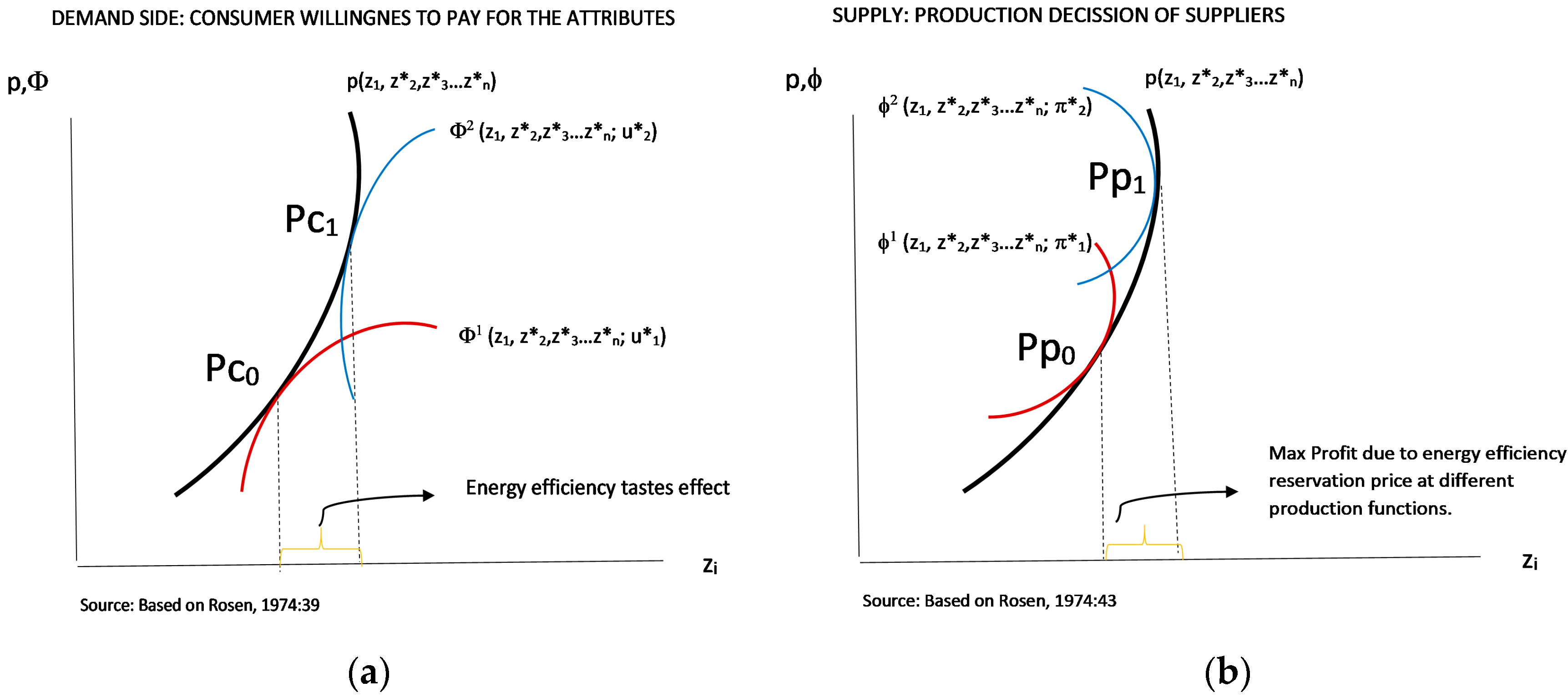
The Rosen [39] model explained this difference clearly, and this can be extended to include energy efficiency as one of the property amenities (Figure 1). Thus, assuming that, in the combined-attribute house price model, energy efficiency is an extra component, and that the rest of the housing characteristics and amenities compose the “envelope” group of features of one house at any location, then z = {z1, z2, …, zn}, with zi measuring the amount of the i-th characteristic contained in a house and z being the particular package of features identifying the particular house. The price also represents that particular package p (z) = p {z1, z2, …, zn}, and the group of characteristics guides both buyers and sellers in a specific location through the number of characteristics, equalizing the differences in the set of hedonic prices. As Rosen stated, “the market clearing prices p (z) are determined by the distributions of consumer tastes and producer costs” [39] (p. 35). Consumers continuously choose among different combinations of z, the function relating prices and characteristics p (z) = p {z1, z2, …, zn}, which are similar in the absence of any alteration of the envelope, such as using additional resources make the house more energy efficient.
Thus, if the value of the green premium depends on consumer behavior, the process of adding value for this characteristic is intrinsically determined by the willingness to pay of green-conscious buyers whose utility curve is modified upon entry to the market by this characteristic. Using Rosen’s [39] (p. 39) definition, the demand behavior is represented in Figure 1a.
On the demand side (Figure 1a), ui is the value function of every consumer at a particular location; this depends on the individual utility function which varies with the available income (y), a bid function (Ф), and the combination of characteristics chosen (U (y − Ф, z1, z2, …, zn) = u). Thus, p(zi) is a function of the minimum price paid in the market for the bundle of characteristic’s unit with z* optimum quantities of each attribute at each implicit price of zi (Pc0). Assuming that z1 is the attribute “energy efficiency”, every consumer represents a different value function; hence, a consumer whose perception is that the house is more energy efficient increases the value of the green component in the envelope (bundle of characteristics), revealing his/her willingness to pay for energy efficiency, jumping the preferred combination from curve red to curve blue, and determining two different fixed-value functions () and the increase in price due to the extra amount of z1 to Pc1. The Ф values are defined as convex functions of every combination of features, while the price function is a non-sufficient convex function representing the first-order condition. “If it is sufficiently regular and convex everywhere, higher-income consumers can purchase a greater number of all characteristics” [39] (p. 40).
On the supply side (Figure 1b), the housing suppliers exhibit an offer function (ф (z1, z2, …, zn; π, β)) which indicates the unit price they are willing to accept at a constant profit (π) on various investment designs. It is assumed that the supplied characteristics in every design meet market characteristics—the implicit prices—to reach the equilibrium at the maximum price, such that one unit could be supplied at similar β coefficients. They maximize their utility at the maximum profit π, which will vary if they include large investment on energy efficiency to increase z1. The increase in the latter is transferred into a higher asking price (from Pp0 to Pp1), with the latter including the expected producer benefits derived from the larger energy investment costs.
Note that Pc0 is not necessarily equal to Pp0, and that Pc1 is not equal to Pp1 (nor the attribute prices), and that the Pcs will be transformed into Pps after the negotiation process. In addition, the mentioned prices (Pc0, Pp0, Pc1, Pp1) reflect different shadow prices of attributes when the focus of the analysis shifts from the demand or the supply side, although both should meet the market hedonic price functions to reach equilibrium (and be transacted) in the presence of sufficient supply to meet the demand. Rosen [39] (p.44) pointed out that “p(z) represents a joint envelope of a family of value functions and another family of offer functions”. Hence, the focus adopted by this research is key to the empirical analysis and interpretation of results, in order to disentangle the meaning of the green premium and to identify whether a green premium (understood as the willingness to pay for energy efficiency) or a green-expected profit exists (understood as the benefit expected derived from an improvement in the energy efficiency of the property).
The literature rarely makes such a distinction, and most papers use the concept of shadow prices as a proxy for the willingness to pay, independently from the observed price, for green characteristics.
3.2. Empirical Model
The empirical literature identifies the price of a particular house (Phit) in terms of the shadow prices of its characteristics (Xkit) at a micro level, which are controlled by location (αi), as a way to capture the willingness to pay. In this framework, green would be valued as an extra “x” component (Equation (1)).
This estimation of shadow prices tries to directly capture the hedonic market prices, without taking into account the components that equilibrate the supply or demand conditions (that is, π or u in the former explanation), but focuses on the difference depending on the type of price observation used. Otherwise, the calculated shadow prices may refer to different equilibrium positions and, therefore, may not be comparable.
From the supply side, the attributes included in the offer function are those with a particular cost that can be evaluated. In the case of housing, construction is a complex activity which creates several attributes at the same time and with the same costs. For example, the market values, in a different way, the floor area or number of rooms; hence, the existing literature tends to include every attribute in a hedonic model from the demand perspective. However, as equilibrium should exist, several variables capturing the same information could bias the shadow prices by introducing problems of multicollinearity or endogeneity in the hedonic model, requiring the use of alternatives to Ordinary Least Squares (OLS) methods to estimate shadow prices (using Instrumental Variables –IV- or Generalised Least Squared -GLS-). This is an important consideration in evaluating green premium. In the case of energy, it is technically demonstrated that particular characteristics such as construction quality, age, and house size and type affect consumption and CO2 emissions (thus, including all of them in a model would result in endogeneity problems rather than just multicollinearity). The current literature weakly refers to this problem in the hedonic definition of green premium (in Appendix C, such a relationship is estimated in order to quantify the endogenous effect of those characteristics).
3.3. Database Sources and Matching Process
This research seeks to find empirical evidence of a green premium in relation to the housing market in Alicante province, Spain, using data contained in EECs and a valuation database providing price information. In Spain, an official EEC is compulsory and must be presented when a house or a building is being transacted (for either sale or rent), in refurbishments or rehabilitations, and for public buildings since June 2013 [40]. The EECs do not collect any economic variable, such as prices or rents.
Although the central government in Spain took the initiative in creating a program for the estimation of energy ratings and the generation of certificates, its application and control falls within the scope of the autonomous communities (Spanish regions). However, most of the regions do not publish the full EEC information in a usable manner and, commonly, the information contained in the available databases is limited.
The EEC data collect all certificates issued in six Spanish provinces (Alicante, Valencia, Castellón, Barcelona, Rioja, and Navarra), which allows for comparison in rate classification, while the valuation database only refers to Alicante. The EEC data contain few observations in the A to D categories, which is the reason for the aggregation of A, B, and C into one category in the empirical exercise (following References [10,17,35]). Comparing the classification of observed houses among them, the evidence identifies that coastal Mediterranean regions in Spain present few houses classified between A and D than in the interior areas. In Alicante (the database of reference for the sample used in this paper), this represents 4.7% of houses, while values in Castellón, Valencia, Barcelona, Navarra, and Rioja are 4.9%, 8%, 14.3%, 32.12%, and 22.7%, respectively, showing an initial evidence of the climate requirements on energy efficiency at home. The low representation of properties rated A–D is notable, but it could be a common pattern in the coastal areas, which will be confirmed when more evidence appears in the literature.
On the other hand, transactions are not published in Spain as micro data (there is no detailed information for every particular transaction), nor are they associated with the energy efficiency. As a consequence, it is not possible to find a unique database with the required variables to evaluate the green premium.
This paper builds a database for this purpose. It matches the EEC and the valuation databases with the Cadaster in order to have precise information about the location and building characteristics. The Cadaster database allows the allocation of geo-referenced properties identified in the EEC and in the valuation databases. The matching results give a geo-referenced database with a large number of characteristics, as shown in Table A1 (Appendix A). Details of the databases used are as follows:
- (1)
- Energy certificates, sourced from a Government Agency, IVACE [41] (Instituto Valenciano de Competitividad Empresarial), contain detailed information on each transaction and its energy characteristics, and a limited number of housing features (Table A1, Appendix A). The total number of energy certificates issued for housing in the Alicante province is 28,558, and the database contains basic information such as size, KWh energy consumption, CO2 emissions, property age, floor, type of housing, and emission/energy consumption rating. The variables used for matching waere the Cadastral reference and the geo-reference, which were also included in the EEC database.
- (2)
- The Cadaster database gives information about the block where the house is located and the specific geometries (floors, orientation, position in the street), including technical information on the buildings with details of the property location at the building level, allowing information on size, location, limits, levels, orientation, construction quality, age, type (single-family, multi-family, or block houses), and other technical characteristics to be accessed [42]. The extraction and exploitation of cadastral data was performed following the methodology developed by Mora García [43] (pp. 85–111).
- (3)
- The database of housing valuations, detailed in previous research [44], contains a large number of observations of houses listed for sale, including asking prices, attributes at various levels, and a geo-reference for each property. As a valuation database, information is provided relating to the value of the subject property and comparables. Only information about the latter is used in this analysis in order to guarantee that the asking price is used and not the valuation. The valuation database for Alicante province contained 517,671 observations, but only 24,138 were geo-referenced. The latter were used in the analysis.
Note that the use of asking price in this paper does not reflect any limitation on the study; rather, it reflects the use of the precise price observation from the supplier side in the market, as explained later. Evidence about the differences between asking prices and transaction prices differs in the literature [45] and is largely explained in Reference [44].
Spatial geometries (at the building level) were built based on the Cadaster database information in order to serve as the elements to match both energy certificates (ECC) and valuation databases. Each EEC observation was assigned to every geometry (using the Cadaster reference), while the observations on the latter were also assigned using the geo-reference. Spatial programming was used to identify the observation falling in every spatial geometry, matching two sets of observations where the properties are located using a spatial analysis tool. The database construction process is explained in Appendix B.
The final database contained 8949 matched EECs—listing properties which were drawn from 24,138 comparables in the valuation (control) database and 28,558 usable EECs (treatment). The merged data and main descriptive statistics are shown in Table A1 (Appendix A).
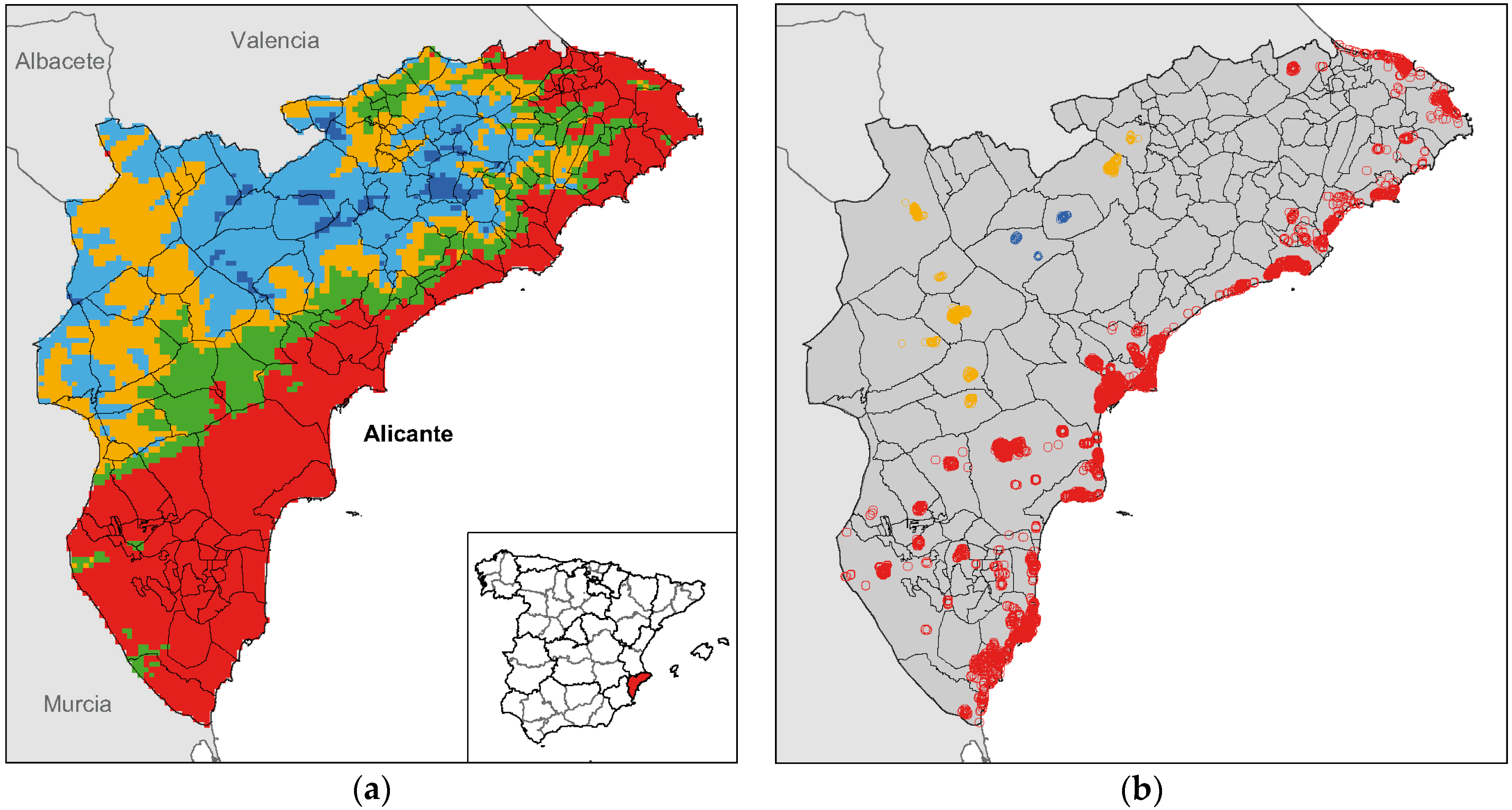
The climatic zones (Figure 2) in the Alicante province are technically classified into three categories (left panel) according to the severity of the summer and winter climates by the Spanish Technical Code [46], with the right panel showing the spatial distribution of observation across the province.
The three climatic areas were zone 1, coastal (red, with 91.9% of the observations); zone 2, interior, soft (an interior area with no extreme weather, shown in orange, with 7.2% of observations); and zone 3, interior, hard (the interior area with harsher temperatures, shown in blue, with 1% of observations). The average energy consumption and CO2 emissions are consistent within each zone, with lower values for climatic zone 1 (coastal region) and higher values for climatic zone 3 (Table 2).
4. Results
4.1. Model for Green Premium in Alicante
The model adopted in this paper was hedonic-based with the green variables considered as an additional attribute. As the focus was on the supply side, the model included technical attributes relating to building and construction quality. The interpretation of the green parameter was also from the supply side and was considered as a measure of the perceived market price generated by the increase in energy efficiency (Equation (2)).
The X-matrix contains the housing attributes obtained after matching the three databases. “Green” refers to the energy indicator (measuring either energy consumption or CO2 emissions) and Phit is the price of a particular housing unit. The intercept is divided into two types, α0 which is a constant across regions, and ∑γiFEi which is the region-specific constant term, time-invariant and capturing specific features of housing consumption across locations. FEi is the dummy variable for the i-th urban level (autonomous city, dependent city, county capital, and province capital) in Alicante (FEi = 1 for i = j; otherwise, FEi = 0 for i ≠ j). The parameter γi is the time-invariant individual effect allowing for region-specific characteristics (location, local conditions, and economic structure) in the model. The variable climatic controls by climatic area, while εit is the error term.
The model was estimated using two methods which are applied sequentially: pool Ordinary Least Squares (pool-OLS) and pool Two-Stage Least Squares (pool-2SLS, IV estimator). The latter was driven by the suspicion of endogeneity between energy consumption and some of the control variables (Table A2, Appendix C, shows the model estimated using pool-OLS with energy consumption/CO2 emissions and the housing attributes to support this suspicion). Hence, a two-step least-square method was used. The instruments in the robustness exercise were selected from the attributes included in the database, among those which fulfilled instrument requirements, rather than building the instruments. The variables of interest were those which captured energy consumption and emissions which served to estimate the green premium associated with house price. Such a premium could determine the profitability of potential retrofitting of a house to a more energy efficient nature. The model took the functional form of a linear semi-log equation including a non-linearity in age.
4.2. Pool-OLS Model
The first set of analysis in terms of assessing the presence and effect of a green premium was tested using a simple OLS model in the merged panel, estimating Equation (2) in a semi-log functional form. The component “Xk” was the attribute matrix (a control variable) and included 33 attributes with neighborhood characteristics (type of neighbor, first or second residence area, accessibility measured through access to the bus and train station, quality of services such as retail, health equipment, income level, and population density) and group or building characteristics where the house is located (type of building, density, urbanization quality, number of lifts, construction quality) and house characteristics (improvements, type of house, age, age², size of the house and uncovered areas, number of bedrooms, bathrooms, total rooms, whether it is a first or second residence, orientation, views, whether it is a public house or rented house). Table 3a and Table 3b contain the results of the nine estimated models, and Table 4 shows the estimated parameters for the control variables. The results were very consistent among the nine estimated models. The location component in this model was captured using urban type, which classified the urban areas into four categories (as in Reference [44]). The model also was estimated including spatial correlation components. The finding that the energy consumption was not spatially correlated led to choosing the functional form following parsimonia. Results are available under request.
The two variables of interest were the energy consumption/CO2 emissions controlled by climatic areas. The EEC provided the total consumption in kWh/year and CO2 emissions were estimated based on housing characteristics using a complex technical model. Both variables reflected the dwelling energy efficiency and were highly correlated (Corr (lkwh. lCO2) = 0.924); thus, they could be used alternatively as a measure of energy. An additional energy efficiency measure was the rate assigned to the house by the EEC.
Accounting for total consumption and emissions, the model was allowed to estimate the price elasticity of energy efficiency in Models 1 and 2 (Table 3 shows the energy parameters, and the results for the control variables are shown in Table 4). The results support previous evidence of a strong significant negative association between energy consumption and housing asking prices. Both estimated parameters (for energy consumption and emissions) show consistent values around −0.03 suggesting that a 1% reduction in energy consumption is associated with higher house prices by 0.031% (0.029% if there is a 1% increase in CO2 emissions).
Regarding EEC rating (Models 3 and 4, Table 3a; note that, in this case, the model captured how much of an increase in price there was for a house of one energy category referred to the omitted one), evidence was found for a green premium in the other energy bands: 1.8% for properties in band F relative to G, and a 1.1% premium in E-rated properties relative to F-rated properties, implying that reducing CO2 emissions in a house rated F increases house price by 1.8% relative to a house rated G, and reducing them in a house rated E increases price by 1.1% relative to a house rated F. If electricity consumption was measured, consistent results were found when improving the consumption from G to F, indicating a house price increase of 1.8%. These results suggest that the effect of improving a poorly energy efficient house to a better one is larger for houses with lower levels of energy efficiency.
The three climatic zones, included in the model as dummies (omitting zone 3, Model 4 Table 3a), showed consistent evidence of different price effects associated with location. In this context, there was a premium for house prices in the coastal area of 17% and a discount in the interior soft area of −15.6, both relative to the hard interior zone. That is, prices of housing located in the coastal areas were, on average, 17% more expensive than those located in the interior hard (note that soft refers to the areas located in the interior with cold weather, while hard refers to those also located in the interior but with harder and more extreme weather in the summer and winter).
As these parameters could capture the location effect and not the energy effect, a set of interactions between both variables was included in Models 5 to 9 (Table 3b). Firstly, the joint variables between energy consumption/emissions and zones gave six combined variables (3x2 variables with zone ixlkwh and zone ixlCO2) in Models 5 and 6. Secondly, a combination between ABC to G rates by zone (5x3 merged variables with zone ixkwh rate j) underpinned Models 7 to 9.
The first set of combined energy consumption variables tested the energy effect on house prices by climatic zone (Models 5 and 6), that is, the response of prices to the energy rating depending on the energy consumption/CO2 emission level. The results support previous evidence with robust parameters (signs and statistical significance) and values that empirically highlight a better energy efficiency of F-rated houses relative to G, and increases in house prices between 2.1% and 1.9% (according to the energy or emission level in each zone). Note that, upon controlling by energy consumption/CO2, the model failed to find empirical evidence of the price effect when dwellings improved efficiency from F to E, as captured by the general model. The interpretation of the energy consumption parameters by climatic zones (Model 5) was a bit more complex, as they reflected the price responses to the energy consumption level in different climatic areas associated with the energy rate. The energy consumption effect on house prices highlighted a larger price effect in climatic zone 2 (interior soft) of −4.6% (a reduction in energy consumption by 1% associated with an improvement in the housing rate, increased the house prices by 4.6%), and a (lower) −1.6% price effect in climatic zone 3 (interior hard). As the models were controlled by characteristics, these differences could only be due to the general environment or quality level in the stock rather than to individual features. Parameters for zone 1 were positive and statistically significant at 5% in Model 5 (but not in Model 6, associated with CO2 emissions), suggesting that the price effect was a 1.5% increase in prices when consumption increases were associated with an improvement on energy efficiency in the dwelling. This result was an apparent anomaly and contrary to other evidence in the literature. However, as houses are located in coastal areas with a warm temperature in most of the year, this response would be evidence of a rebound effect, that is, because the house is more efficient, the user could increase energy consumption in air conditioning, for instance. The parameters were consistent with those in Model 6 using CO2, emissions with larger effect on reducing emissions in zone 2 (−7.2%).
Models 7 to 9 included the interactions of energy consumption rates and climatic zones in order to see the differences among climatic zones associated with each rating. The three models omitted one zone each. The results were consistent with the previous finding. Model 7 (Table 3b) parameters showed a price premium for houses between 16.2% and 18% in zone 1, and a discount between −13% and −17.7% in zone 2 (consistent with the location results in Model 3), both relative to zone 3 at all energy rates, which can be interpreted as differences in prices at the same level of energy efficiency.
Note that, in the coastal area (zone 1), a systematic result appeared to suggest that a larger price effect occurred in dwellings rated F to D, and not in A to C as expected, while, in the other two zones, the larger (negative) differences in prices (at every rate level) appeared at the lowest rate of G, as expected. Results were robust and consistent, suggesting that, in the coastal area, a minimum investment to improve energy efficiency could have a large price effect and that, consistent with the weather, better energy-efficient homes are not appreciated in the warm areas. This suggests that the effect of expenditure for energy improvement in the lower-rated houses, considering the same absolute energy savings, could be transmitted differently between expensive and cheap markets and could have a strong green premium effect in colder areas and the opposite effect. For instance, expected energy savings capitalized at €10,000 could have a different relative (but the same absolute) price effect on a €100,000 dwelling compared to a €1,000,000 dwelling.
Another interpretation of parameter results would be that the improvement in energy efficiency had the maximum effect on house prices in less energy-efficient properties, for example, band F relative to band G, or band D relative to E, which suggests a high value of energy retrofitting in the extreme dwelling quality.
In the case of zone 2 (an area which is intermediate in terms of weather), the discount was at its maximum for the lowest-banded properties (−17.7%) and at a minimum for D-rated properties, suggesting that an improvement from G to D in zone 2 relative to zone 3 reduced the discount on house prices by 2.3% (from −15.5% to −13.2%).
In terms of prices and energy efficiency (Model 9), zone 2 showed larger discounts, while zone 1 showed the lowest. Thus, if zone 2 was omitted (in Model 8), the green premium in zone 2 driven by any improvement in energy efficiency would increase housing prices from 29.9% to 34.4%, more so than prices in zone 1, showing strong market incentive to invest in energy efficiency in this zone; that is, housing prices after retrofitting would rise around 34%, if the investment is made in zone 2 rather than in zone 1.
In the last three models, the parameters were highly significant (1% in zone 1 and 1% and 5% in zone 2) with the exception of A to C bands in zone 3, possibly due to data constraints.
4.3. Two-Step Model
ECC ratings were estimated based on physical characteristics of housing, as including them into the model as regressors would generate endogeneity problems. There is little debate in the literature about whether the statistical relationship between energy rating and quality or size (for instance) exhibits multicollinearity or endogeneity.
Following this idea, for robustness, a second analysis re-estimated the model using an instrumental two-step method. The key issue here was how to find proper instruments to approach the behavior of energy rating or the physical characteristics (normally scarce in price databases). Thanks to the huge database built by matching three different databases in this paper, it was possible to find instruments for most of the model’s independent variables.
The selection was made using variables (as instruments) having higher correlation to every regressor in order to strongly capture their relationships in the first stage. Table 5 shows the pairs of variables (covariates and corresponding instruments), along with their correlations and significant tests.
The instrument selection in IV models constitutes a debate in the literature, though there is general agreement that they should be chosen using theoretical considerations, as well as their statistical dimension [47,48]. The strategy in this paper was to choose highly correlated variables containing similar information but at different urban levels (see analysis in Appendix C and Table A2). The variables were then paired (subject covariate and instrument), and only those which matched with another variable were included as instruments in the two-step least-square model. To illustrate this further, for an apartment block, the instrument chosen was a building in a closed block; for house age, the instrument used was the building age. The pairs of variables and their correlations are included in Table 5 (a Sangan–Hansen test of over-identified restrictions was run using the results. SH_test = −34.13, rejecting the null hypothesis of over-identification).
Equation (2) was estimated using a two-step least-square method including endogenous attributes identified with an instrument. The results show a lower number of statistically significant housing characteristics affecting prices in the presence of energy consumption. Size, income, number of bathrooms, and being in a building block positively affected house prices, while rented housing and being in the first residence area had a negative effect on prices. The results of the sensitivity of prices to changes in energy consumption are consistent with the previous results and support the idea of around −3% as the green premium for the energy consumption reduction as reflected in house prices. The two-step model failed to find evidence of a green premium associated with energy rates, as none of the IV estimators of energy rating were statistically significant in any of the estimated models.
The 3% green premium in house prices on average for the Alicante province is consistent with other literature results, and suggests that houses with lower energy consumption are worth 3% more than those that are less efficient. This interpretation reflects the supplier perspective (asking prices include the expectation of benefits as highlighted in the theoretical section of this paper); that is, owners offering a house overvalue houses with lower energy consumption by 3%, an interpretation that agrees with Rosen [39]; however, it cannot be understood as the price change due to the energy savings, as the real consumption is not observed in the EEC. This interpretation differs from those studies using asking prices to identify the green premium. (See Table 6)
5. Conclusions and Policy Implications
This paper analyzed the existence of a green premium in house prices in the Alicante province, Spain. Following Rosen’s [39] theoretical explanation of hedonic prices, the paper adds to the debate about the meaning of green premium obtained using asking prices, which refers to the landlord estimation of energy improvements in the house and the expected house price in the market.
The significance of this paper is an advancement in the knowledge on green energy impacts on house price through two dimensions: (1) the different premiums by climatic area, and (2) debating endogeneity in energy hedonic models. It also adds evidence of southern European markets from the energy perspective.
An instrumental method was also applied, seeking bias resulting from the (potentially) endogenous relationship between energy consumption and physical housing features which can affect the level of the green premium resulting from the hedonic regression. The empirical evidence in this paper found more consistent results in the panel IV model than in the pool-OLS model, although it also found the existence of endogenous relationships between some of the housing attributes (normally included in the hedonic green models) and energy consumption (KWh) or carbon dioxide emissions (CO2). These results suggest three main findings: (1) the results are robust; (2) energy ratings are not a simple combination of characteristics, but rather, a technical reflection of the building energy features; (3) the hedonic model estimations made in a pool are accurate in capturing the market incentives for energy retrofitting.
The analysis showed a green premium of 3% on housing (asking) prices in relation to consumption/emissions; in the case of improvements, a partial green premium exists when improvements increase the EEC rating from G to F (1.8%) and from F to E (1.1%). Significantly, when parameters were recalculated using the IV method, the 2SLS estimators also supported a premium of 3% in house prices associated with lower energy consumption, and failed to support the existence of any effect coming from the energy efficiency ratings. This suggests that asking prices robustly capture energy consumption and emissions measured as continuous variables; however, the rating classification, resulting from the algorithm used by the official EEC generator, does not show endogeneity with prices, and their green effect is better captured using simple models.
The paper provided evidence of different green premiums associated with each climatic area. We found evidence of a potential rebound effect in the coastal region (better energy-efficient units associated with larger prices and a positive increase in energy consumption) and a clear green premium in colder areas. The former suggests that the retrofitting costs would be transmitted to an increase rather than a reduction in energy consumption costs, as a way of dealing with the extreme hot weather. This result is relevant in the context of climatic change.
The fact that a larger green premium appeared in the intermediate zones (−4.6% based on consumption; −7.2% based on emissions), rather than in colder zones (−0.6% and −3.1%, respectively), shows a higher sensibility in regions with more weather instability and a potentially worse isolation system installed in the housing stock.
The differences in green premium among climatic areas captured by the interaction parameters reached almost 30% between the two extreme areas, confirming the intuition that the sensibility of housing (asking) prices to energy efficiency is one-third lower in the hotter regions. The fact that the extreme regions did not show a larger effect on prices indicates better insulation features in zone 3 stock.
The empirical results obtained in this paper have relevant policy implications. Firstly, by quantifying market incentives, it raises the possibility of precisely calculating the scope of policies focused on energy efficiency renewal, allowing to discriminate the amount of financial support according to the size of the market response. The ability to differentiate between energy efficiency from a buyer’s or owner’s perspective is potentially beneficial, as parties could show diverse market perception of incentive intensity. The green premiums using hedonic models identifying the origin of the price incentive (supply or demand) will support a more precise identification of public policy promoting the energy efficiency (and the channel to implement it), as well as avoiding mistakes in the estimation of the cost–benefit calculation in the private investment process.
Secondly, as the price signals showed different levels depending on climate areas, energy efficiency incentive policies should discriminate between them, modulating the aid according to their price responses. As green premium is a market response, any policy should define the public plans according to the market mechanism in order to achieve the EU energy objectives.
Thirdly, the results suggested that the rating classification within the EEC is not clearly identified for the market players. If the A–G rating is made in order to classify the efficiency of the houses, and the market does not identify them, the rating should evolve toward a more comprehensible manner allowing market forces to recognize and price them.
Lastly, the rebound effect could be an issue to deal with in the context of climate change policy. The hottest regions (which initially showed lower energy consumption and emissions) will use increasing energy to adapt to temperatures at home, increasing consumption as temperatures rise.
In summary, this article follows the methodology in the existing literature on estimating market incentives for investment in energy retrofitting. It adds knowledge about the situation in southern European regions, and shows the existence of different incentives depending on the climate area concerned. As the article demonstrates, analyses focusing on market incentives should take into account climatic areas to obtain more accurate results and, thus, be able to correctly target policy measures defined to increase incentives for energy improvements in housing.
Author Contributions
All authors contributed equally to this work. All authors wrote, reviewed, and commented on the manuscript. All authors read and approved the final manuscript.
Funding
This work was supported by the project RentalCal (http://www.rentalcal.eu/) funded by the European Union within the framework of H2020-EE-2014-2015: H2020-EE-2014-3-MarketUptake. The content of this publication is the exclusive responsibility of its authors and does not necessarily reflect the opinion of the European Commission.
Acknowledgments
We acknowledge the support of Professor Stanley McGreal from Ulster University for the different versions of this article. Finally, we thank the EEC register of the Generalitat Valenciana (IVACE-energía) for data provision.
Conflicts of Interest
The authors declare no conflict of interest.
Appendix A. Basic Statistics

Table A1.
Basic Statistics.
| DB | Characteristics | Mean | Median | SD | Asymmetry | Kurtosis |
|---|---|---|---|---|---|---|
| EEC DB | C_year_CONS | 1986.5 | 1991.0 | 209.2 | 66.5 | 5777.4 |
| C_EMIS_CO2 | 54.4 | 43.0 | 198.0 | 30.2 | 1020.2 | |
| Ln_co2 | 3.8 | 3.8 | 0.5 | 1.8 | 18.2 | |
| C_EMIS_rate: | ||||||
| Emis_A | 0.0 | 0.0 | 0.0 | |||
| Emis_B | 0.0 | 0.0 | 0.0 | 47.3 | 2233.5 | |
| Emis_C | 0.0 | 0.0 | 0.1 | 16.4 | 266.3 | |
| Emis_D | 0.0 | 0.0 | 0.2 | 5.1 | 23.6 | |
| Emis_E | 0.5 | 0.0 | 0.5 | 0.2 | −2.0 | |
| Emis_F | 0.1 | 0.0 | 0.4 | 2.0 | 2.0 | |
| Emis_G | 0.4 | 0.0 | 0.5 | 0.6 | −1.6 | |
| C_CONS_KWH | 206.8 | 170.9 | 678.7 | 37.9 | 1609.9 | |
| Ln_kwh | 5.2 | 5.1 | 0.4 | 1.3 | 15.5 | |
| C_CONS_rate | ||||||
| Cons_A | 0.0 | 0.0 | 0.0 | |||
| Cons_B | 0.0 | 0.0 | 0.0 | 47.3 | 2233.5 | |
| Cons_AB | 0.0 | 0.0 | 0.0 | 47.3 | 2233.5 | |
| Cons_C | 0.0 | 0.0 | 0.1 | 15.5 | 237.0 | |
| Cons_D | 0.0 | 0.0 | 0.2 | 4.9 | 21.6 | |
| Cons_E | 0.5 | 1.0 | 0.5 | 0.0 | −2.0 | |
| Cons_F | 0.1 | 0.0 | 0.3 | 2.2 | 2.9 | |
| Cons_G | 0.3 | 0.0 | 0.5 | 0.7 | −1.4 | |
| Cadaster DB | E_INE_MUN_code | |||||
| E_year_CONS | 1988 | 1991 | 17.4 | −0.9 | 1.4 | |
| Age | 25.0 | 22.0 | 17.4 | 0.9 | 1.4 | |
| age square | ||||||
| E_Nº house units | 75.6 | 36.0 | 99.8 | 3.0 | 13.9 | |
| E_floor_SR | 6.8 | 6.0 | 5.3 | 3.2 | 13.5 | |
| Building type (Cadaster): | ||||||
| Bt1_ap_open block (B1_ap_Oblock) | 0.3 | 0.0 | 0.5 | 0.7 | −1.5 | |
| Bt2_ap_closed block (B2_ap_Cblock) | 0.6 | 1.0 | 0.5 | −0.3 | −1.9 | |
| Bt3_house_singlefam (B3_SF_h) | 0.0 | 0.0 | 0.2 | 4.8 | 21.5 | |
| Bt4_house_urbanization (B4_SF_urb_H) | 0.1 | 0.0 | 0.3 | 3.4 | 9.8 | |
| Bt5_Rural house (B5_rural_h) | 0.0 | 0.0 | 0.0 | 54.6 | 2979.7 | |
| Floor (over the land level) | 5.0 | 2.0 | 14.4 | 6.1 | 36.6 | |
| Years from retrofitting, Retrof_year | 24.3 | 0.0 | 218.9 | 8.9 | 77.1 | |
| Type of refurbishment: | ||||||
| Full refurbishing (building), F_refur_build | 0.0 | 0.0 | 0.0 | 31.5 | 989.9 | |
| Total refurbishing(house), T_ref_sh | 0.0 | 0.0 | 0.0 | 38.6 | 1487.3 | |
| Full Improvements, RF_improv | 0.0 | 0.0 | 0.1 | 18.1 | 326.6 | |
| Small improvements, RF_small | 0.0 | 0.0 | 0.1 | 11.5 | 130.7 | |
| Tot building floors | 1.1 | 1.0 | 0.3 | 5.1 | 32.8 | |
| Valuation DB | date | |||||
| Type (SF, MF, Block), type | ||||||
| Nº housing units in the building, N_dweel | 28.8 | 16.0 | 51.8 | 18.6 | 639.3 | |
| Age | 11.0 | 7.0 | 10.6 | 0.9 | −0.1 | |
| Age_new2 (squared) | 234.7 | 49.0 | 355.2 | 3.0 | 30.7 | |
| M2 (usable), size | 93.2 | 90.0 | 29.5 | 1.1 | 4.1 | |
| M2 (non covered areas like patios) m2_noncover | 5.8 | 0.0 | 17.6 | 4.7 | 30.6 | |
| Urbanization quality, Urban_Q | 1.0 | 0.0 | 1.4 | 1.1 | 0.2 | |
| Total floors in building, floor | 7.0 | 6.0 | 4.4 | 2.4 | 8.4 | |
| Nº bedrooms, N_bed | 2.6 | 3.0 | 0.9 | 4.4 | 149.3 | |
| Nº bathrooms, N_bath | 1.5 | 2.0 | 0.5 | 0.4 | −0.2 | |
| Type of urban area, Urb_type: | ||||||
| TN_dependent, Urb_Dep | 0.1 | 0.0 | 0.3 | 3.1 | 7.6 | |
| TN_autonomous, Urb_Auton | 0.6 | 1.0 | 0.5 | −0.3 | −1.9 | |
| TN_county capital, Urb_County | 0.1 | 0.0 | 0.3 | 2.2 | 2.7 | |
| TN_provice capital, Urb_prov | 0.2 | 0.0 | 0.4 | 1.4 | 0.0 | |
| Nº inhabitants, POP | 127,285 | 84,626 | 132,756 | 4.4 | 73.9 | |
| Main Economic Activity in town, Economy | 3.5 | 3.0 | 1.1 | 0.0 | −0.8 | |
| Population growth in town | 1.8 | 2.0 | 0.4 | −1.8 | 1.5 | |
| Rural, sub.urban, or urban feature | 3.0 | 3.0 | 0.0 | −37.4 | 1547.3 | |
| Type of residence neighborhood: | ||||||
| 1st residence neighborhood, D_1_residence | 0.6 | 1.0 | 0.5 | −0.5 | −1.8 | |
| Mix residence neighborhood, D_mix_res | 0.1 | 0.0 | 0.3 | 3.3 | 8.9 | |
| 2nd residence neighborhood, D_2_residence | 0.3 | 0.0 | 0.5 | 0.8 | −1.4 | |
| Dummy: if main house is in second neighborhood, D_ifsecond | 0.0 | 0.0 | 0.1 | 7.7 | 56.8 | |
| Income level in town (from 1 very low to 7 very high), Income | 4.4 | 4.0 | 0.8 | 0.5 | 2.1 | |
| Population density in town (1 = low. 3 = high), Pop_dens | 2.6 | 3.0 | 0.5 | −0.4 | −1.6 | |
| Consolidation of urban area (max 100%), Cons_urb | 88.8 | 90.0 | 10.0 | −5.2 | 41.1 | |
| Population pattern (1= paralyzed. 6 = full), Pop_trend | 3.3 | 3.0 | 0.8 | 2.4 | 4.7 | |
| Renovation degree in the neighborhood (max 100%), renov | 11.5 | 10.0 | 11.5 | 1.8 | 5.2 | |
| Roads quality (0 = no. 4 = very good), Q_road | 2.8 | 3.0 | 0.4 | −1.3 | 1.4 | |
| Retail quality in the area (0 = no. 4 = very good), Q_retail | 4.5 | 5.0 | 0.9 | −0.7 | −0.4 | |
| School quality in the area (0 = no. 4 = very good), Q_school | 4.0 | 4.0 | 0.5 | −3.8 | 24.6 | |
| Religious quality in the area (0 = no. 4 = very good), Q_relig | 4.0 | 4.0 | 0.5 | −4.2 | 25.5 | |
| Leisure quality in the area (0 = no. 4 = very good), Q_leis | 4.0 | 4.0 | 0.4 | −2.7 | 23.1 | |
| Sport amenities quality in the area (0 = no. 4 = very good), Q_sport | 4.0 | 4.0 | 0.4 | −2.7 | 23.1 | |
| Health service quality in the area (0 = no. 4 = very good), Q_health | 4.0 | 4.0 | 0.4 | −3.4 | 24.2 | |
| Bus (0 = does not. 5 = interurban network) | 4.2 | 4.0 | 0.6 | −1.5 | 9.9 | |
| Train (0 = no train. 1 = train nearby. 2 = train in the municipality) | 1.3 | 2.0 | 0.9 | −0.6 | −1.6 | |
| metro (0 = does not. 5 = interurban network) | 0.0 | 0.0 | 0.1 | 44.4 | 2016.5 | |
| Nº lift in building, Lift | 1.1 | 1.0 | 1.1 | 2.5 | 16.3 | |
| Retail quality in the subject property neighborhood (0= no. 5= very good), Q_retail_neigh | 4.4 | 5.0 | 0.9 | −0.6 | −0.7 | |
| Income level in building where subject property is located (from 1 very low to 7 very high), Income_dwel | 4.4 | 4.0 | 0.8 | 0.7 | 1.7 | |
| Population density in neighborhood (1 = low. 3 = high), popdens_neigh | 2.6 | 3.0 | 0.5 | −0.5 | −1.3 | |
| Orientation (1 = north/worst. 8 = southeast/best) | 5.2 | 6.0 | 2.3 | −0.6 | −0.9 | |
| Views (0 = very bad. 6 = exceptional) | 2.7 | 2.0 | 1.0 | 1.0 | −0.1 | |
| Construction quality (1 = very bad. 6 = very good), Q_constr | 3.6 | 4.0 | 0.8 | −0.6 | 0.3 | |
| Asking Price, Pr | 164,889 | 148,000 | 89,586 | 3.6 | 28.6 | |
| LnPr (log of asking Price) | 11.9 | 11.9 | 0.5 | 0.2 | 1.1 | |
| Asking Price by m2, pr_m2 | 13,045 | 11,496 | 7460.9 | 3.2 | 22.0 | |
| LnPr_m2 | 7.4 | 7.4 | 0.4 | −0.1 | 0.2 | |
| Rent/month (euros), Rent | 161.5 | 132.3 | 148.3 | 6.7 | 62.0 | |
| lnRent | 4.9 | 4.9 | 0.5 | 0.8 | 2.4 | |
| AFFORDABLE HOUSE (0 = private. 1 = vpo before 1978 or free. 2 = vpo no doc. 3 = vpo), afford | 0.3 | 0.0 | 0.7 | 2.2 | 3.9 | |
| If public house = 3, D_public_h | 0.1 | 0.0 | 0.3 | 2.6 | 4.9 | |
| Rented house, D_rent | 0.1 | 0.0 | 0.5 | 4.7 | 21.0 | |
| Type of residence (1 = FIRST. 2 = SECOND RESID), type_res | 1.4 | 1.0 | 0.5 | 0.4 | −1.8 | |
| Dummy: if Main house, D_main | 0.6 | 1.0 | 0.5 | −0.4 | −1.8 | |
| Dummy: if second house, D_second | 0.4 | 0.0 | 0.5 | 0.4 | −1.8 | |
| Nº of exterior rooms, N_exter | 2.9 | 3.0 | 1.3 | 1.1 | 1.3 | |
| Nº of total rooms, N_rooms | 6.1 | 6.0 | 1.6 | 11.3 | 468.3 | |
| ratio_Price_rent (anual) Ptor | 101.4 | 99.3 | 42.5 | 0.7 | 1.9 | |
| Climatic zone. Z_clim | 1.1 | 1.0 | 0.3 | 3.7 | 14.1 |
Notes: Number of observations: 8949.
Appendix B. Matching Database Process. Analytical Details
The merging of the databases was done in two steps.
In the first step, a base of energy certificates + Cadaster was created through merging the information contained in energy certificates, the general data of the buildings, and specific data of the real estate and physical elements obtained from Cadaster. This phase was when the Thiessen polygons were created as explained below.
In the second phase, listings of comparable houses were extracted from the valuation database with 25 characteristics, including specific ones for the dwelling and neighborhood, as well as the geo-reference record. Duplications were removed to obtain unique records of dwellings with the same geographical coordinate. From this coordinate, the corresponding Thiessen polygon and the census section were assigned to each observation.
As for the Thiessen polygons, cadastral building blocks were used in urban areas (so-called masses). On these geometries, grids of points at 20 m were created and almost one million points (915,110 concretely) were generated. These points were intersected with the masses such that they inherited the properties of the mass that contained it. Thiessen polygons (32,285 geometries) were generated over them by merging all polygons with the same mass name. These same attributes of Thiessen polygons were replicated in the database of energy certificates + Cadaster in order to match every observation.
An example of the succession in the geographic identification is shown in Figure A1, Figure A2 and Figure A3. On Figure A1, the Thiessen polygons at the level of blocks or buildings are shown, created for the whole Alicante province and detailed for Alicante city.
Figure A1.
Thiessen polygons in 39 selected municipalities for the Alicante province. This map gives an example of the steps followed to merge the databases. (a) Thiessen polygons built based on the Cadaster database; all polygons built in the Alicante province. (b) Thiessen polygons for the whole province, built at the block level with an example of the Alicante city center.

Figure A2.
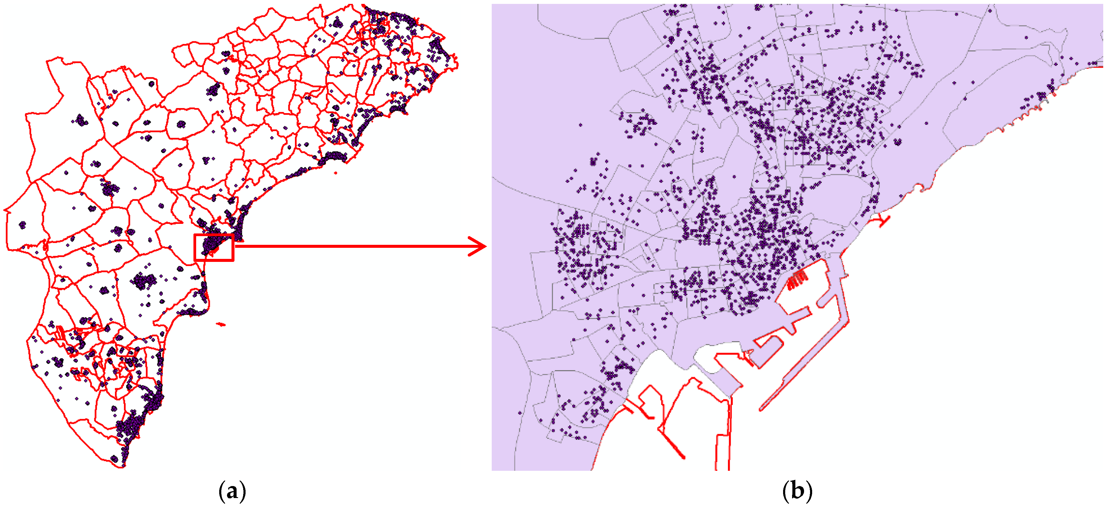
Dwelling transaction geo-referenced data in the Alicante province. The maps show the spatial distribution of the valuation database on the Alicante province (a), with detail in Alicante city (b). The observations are distributed according to the housing stock across the province. Source: Tabimed database.
Figure A2.
Dwelling transaction geo-referenced data in the Alicante province. The maps show the spatial distribution of the valuation database on the Alicante province (a), with detail in Alicante city (b). The observations are distributed according to the housing stock across the province. Source: Tabimed database.

The information contained in the Cadastral database (DB) completed the missing technical information in the energy certificates, as well as in the valuation DB. Some attributes relative to housing were included in the database, such as whether the property is a single-family house or multi-family house, the building density if it was a block, the climatic zone, and a simulation of min and max values for emissions and consumption in order to double-check the information contained in the EECs certificates (allowing to discriminate, for instance, when the certificate was for a building or for a unit). New variables were created with those defined attributes: Cadaster identifier (characteristic E_DGC_MUN); Building type = U if single- or multi-family, V if it is in a block; climatic zone (ZC_zoclima), min and max emission or consumption (ZC_min_EMI, ZC_max_EMI, ZC_min_CON, ZC_max_CON).
Once the polygons were obtained, each property in the energy certificate database was paired using the Cadastral parcel number and located in the map using the geo-reference. This process also allowed identifying each building in every block. Also, using geographic information system (GIS) techniques, every geo-referenced property of the valuation data was “located” on the map where the polygons and energy certificates were already assigned. The richness of the Cadaster database allowed checking the information contained in the EECs and valuations with the building information in order to achieve robust data. Figure A3 shows the Cadaster blocks individually identified in both databases, and two types of points assigned to each one: the EEC observation (points in red) and the listed property (points in yellow). Figure A3a gives a general view of the neighborhood, while Figure A3b illustrates every property observed in the block and how it was not possible to numerically match both geo-reference points, as any single point corresponding to the same house gave different positions in the building.
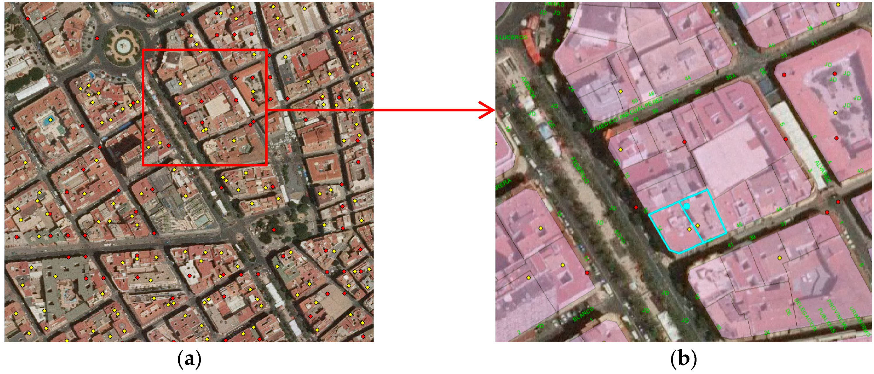
Figure A3.
Dwelling and energy certificate observations in Census section and Cadaster blocks. (a) Distribution of both database observations. (b) Independent building in the Cadaster block. This figure explains graphically how the database merging was done. Through merging the energy certificate database and Cadaster database, one intermediate database was obtained, containing the energy information and building characteristic information with the data geo-referenced (red points). The valuation database was also geo-referenced and allowed identifying the properties on the map (yellow points). Geo-referencing allowed observing both databases on the map. As the geo-reference was not a feasible variable to match both databases, the Thiessen polygons allowed isolating observations falling in the same block, as shown in (b), where the blue square represents the block taken as a reference for matching. Inside each block, the matching was done among pairs of observations which were the same size, or had the same number of rooms or floors.

The second phase of the merging process was to match every EEC/Cadaster built properties with the corresponding property in the valuation database in order to add the appropriate characteristics from the listed properties, including price. The matching principles defined in Smith and Tood [49] were applied here in order to identify the treated properties (those with energy certificates) in both databases. A spatially controlled propensity score was defined, consisting of an algorithm using five time-invariant covariates (size in m2, number of rooms, construction year, building floors, number of dwellings in the building) plus the building or Cadaster block (variable which serves as space control), which sequentially tested the probability that differences in covariates were zero by building. The resulting estimated propensity score assigned to each property matched pairs of treated with untreated houses located in every building, allowing the precise identification of the same properties in both databases when their probability was equal to 0. The propensity score is defined in Equation (A1), following Smith and Tood [49], although the score was defined to adapt the needs of this research.
where Psi is propensity score of pair i; Bl is the Cadaster block or building, with l different buildings; is the covariate k of property i in the treatment group; is the covariate k of property j in the control group; k is the number of covariates (5); l is the number of Cadaster blocks or buildings; and n is the total number of properties in the treatment group falling in every Cadaster block.
The propensity score (Psi) was the probability of matching every pair of observations that met the algorithm with the results of the final DB having the treated observations with a propensity score equal to zero, and untreated property observations with a probability different from zero.
Note that EEC database (treatment group) observations belonged to the period of 2013–2015, while the control group properties belonged to the period of 2007–2012. The difference in the periods was taken into account due to data constraints. The matching method used time-invariant housing attributes, in which time had no effect; however, the assignation of price (which is a time-varying feature) to observations in the treated group indicated that matching created the DB with energy variables and housing prices, representative of the period 2007–2012.
Appendix C. Endogeneity in Hedonic Models Estimating Green Premium with EEC
Energy characteristics in the hedonic models could suffer from the existence of correlations and multicollinearity among the energy features and the physical characteristics. In order to avoid the bias in the parameters generated by a potential endogenous relationship (for instance, the older the house, the more energy consumption in the absence of energy-efficient renovation), this paper explored the existence of potential endogeneity among the building characteristics and how they could endogenously determine the energy consumption.
Housing characteristics were not independent among them. The literature identified how energy consumption depends on multiple factors related to several physical characteristics [30,50], including local climate or housing equipment, quality of construction, isolation, and building envelope features. Building age [29,51] is associated with the level of energy consumption, suggesting that a certain degree of endogeneity could exist when those variables are analyzed together. The literature weakly refers to this problem in the hedonic definition of green premium. The main problem when evaluating such endogeneity is the difficulty to find instruments approaching the statistical behavior of physical characteristics, which are commonly scarce in physical attribute databases (although the EEC normally collects most technical housing features).
This section explores such a relationship. The literature was followed in order to choose the variables potentially determined endogenously. There are two groups of housing characteristics affecting the energy consumption [29]: construction quality, including energy isolation and efficiency system; and construction materials, including physical building attributes, type of housing, and size (m2 or the number of rooms). For instance, an increase in size [34] or number of rooms results in a higher energy consumption [32,52]. Building age also increases consumption. New buildings are more energy-efficient than old ones [34], which are supposedly less efficient [33]. Type of house (single-family or apartment block) also has an influence, with single-family houses showing larger energy consumption [29,30] because of heating and air conditioning needs [32], and a larger size [31]. Quality construction with modern materials improves efficiency [7,10,15].
The test was carried out using the semi-log model shown in Equations (A2) and (A3).
Both estimations were made using a non-linear OLS regression between energy consumption (kWh) and CO2 emissions with the physical housing characteristics listed before. The results (Table A2) suggest around a 7% explanatory power of energy consumption and emissions. Several characteristics were statistically significant, such as age, type of building, improvements, housing density, number of lifts, housing size, the type of neighborhood, being a second residence, and being a public house. Table 3 shows that consistent parameters were obtained using both energy consumption and CO2 emissions. Although the endogeneity was not severe, an IV method was applied in order to re-estimate the endogenous regressors to obtain more consistent and robust results. Controlling for endogeneity requires using a set of instruments to follow the two-step estimation procedure.
Table A2.
Endogenous relationships between energy consumption and housing characteristics.
| ln_CO2 | ln_kwh | |||
|---|---|---|---|---|
| β | t-stud | β | t-stud | |
| C | 4.061 *** | 108.64 | 5.419 *** | 152.27 |
| Age2 | 0.000 *** | 11.64 | 0.000 *** | 11.07 |
| B1_OP_b | 0.010 | 0.85 | 0.012 | 1.06 |
| B3_SF_h | 0.178 *** | 6.90 | 0.207 *** | 8.41 |
| B4_SF_urb_H | 0.121 *** | 5.80 | 0.133 *** | 6.73 |
| RF_Imp | −0.214 ** | −2.47 | −0.188 ** | −2.27 |
| RF_small | 0.012 | 0.22 | 0.031 | 0.59 |
| N_dw | 0.000 ** | 2.51 | 0.000 ** | 2.56 |
| Age | 0.000 | −0.36 | −0.001 * | −1.65 |
| size | −0.001 *** | −4.05 | −0.001 *** | −4.10 |
| size_2 | 0.000 * | 1.67 | 0.001 ** | 2.00 |
| T_floors | −0.001 | −0.85 | 0.000 | −0.27 |
| bed | 0.010 | 1.16 | 0.005 | 0.69 |
| bath | −0.027 ** | −2.06 | −0.024 * | −1.90 |
| Urb_t | −0.058 *** | −8.32 | −0.046 *** | −7.05 |
| 1_res | −0.042 *** | −2.95 | −0.040 *** | −2.91 |
| mix_res | −0.050 ** | −2.44 | −0.047 ** | −2.41 |
| lift | −0.030 *** | −5.16 | −0.031 *** | −5.61 |
| Q_retail | −0.008 | −1.42 | −0.006 | −1.07 |
| orient | 0.001 | 0.43 | 0.001 | 0.35 |
| Q_constr | −0.005 | −0.85 | −0.008 | −1.32 |
| vpo | −0.030 * | −1.93 | −0.033 ** | −2.20 |
| rent | −0.002 | −0.10 | 0.004 | 0.18 |
| rooms | 0.003 | 0.73 | 0.003 | 0.76 |
| Adjusted R2 | 0.067 | 0.069 | ||
| Standard error | 0.437 | 0.416 | ||
| F | 28.990 | 29.854 | ||
| DW | 1.834 | 1.822 | ||
| N | 8948 | 8948 | ||
Notes: *** p < 0.001, ** p < 0.01, * p < 0.05.
References
- IPCC, Intergovernmental Panel on Climate Change. Climate Change 2014: Mitigation of Climate Change; Cambridge University Press: Cambridge, UK, 2014; Available online: https://www.ipcc.ch/report/ar5/wg3/ (accessed on 1 January 2016).
- EU, Official Journal of the European Union. Directive 2010/31/EU of the European Parliament and of the Council of 19 May 2010 on the Energy Performance of Buildings. 2010. Available online: http://data.europa.eu/eli/dir/2010/31/oj (accessed on 1 January 2016).
- Kok, N.; Miller, N.; Morris, P. The Economics of Green Retrofits. J. Sustain. Real Estate 2012, 4, 4–22. [Google Scholar] [CrossRef]
- Eichholtz, P.; Kok, N.; Quigley, J.M. Doing Well by Doing Good? Green Office Buildings. Am. Econ. Rev. 2010, 100, 2492–2509. [Google Scholar] [CrossRef] [Green Version]
- Eichholtz, P.; Kok, N.; Quigley, J. The Economics of Green Building. Rev. Econ. Stat. 2013, 95, 50–63. [Google Scholar] [CrossRef] [Green Version]
- Fuerst, F.; McAllister, P. Green Noise or Green Value? Measuring the Effects of Environmental Certification on Office Values. Real Estate Econ. 2011, 39, 45–69. [Google Scholar] [CrossRef]
- Brounen, D.; Kok, N. On the economics of energy labels in the housing market. J. Environ. Econ. Manag. 2011, 62, 166–179. [Google Scholar] [CrossRef] [Green Version]
- Deng, Y.; Li, Z.; Quigley, J.M. Economic returns to energy-efficient investments in the housing market: Evidence from Singapore. Reg. Sci. Urban Econ. 2012, 42, 506–515. [Google Scholar] [CrossRef] [Green Version]
- Cajias, M.; Piazolo, D. Green performs better: Energy efficiency and financial return on buildings. J. Corp. Real Estate 2013, 15, 53–72. [Google Scholar] [CrossRef]
- Fuerst, F.; McAllister, P.; Nanda, A.; Wyatt, P. Does energy efficiency matter to home-buyers? An investigation of EPC ratings and transaction prices in England. Energy Econ. 2015, 48, 145–156. [Google Scholar] [CrossRef] [Green Version]
- Reichardt, A.; Fuerst, F.; Rottke, N.B.; Zietz, J. Sustainable Building Certification and the Rent Premium: A Panel Data Approach. J. Real Estate Res. 2012, 34, 99–126. [Google Scholar] [CrossRef]
- Eurostat, Statistical Office of the European Union. Energy Statistics-Supply, Transformation and Consumption. Available online: https://www.eea.europa.eu/data-and-maps/data/external/energy-statistics-supply-transformation-and-consumption (accessed on 1 January 2016).
- Soriano, F. Energy Efficiency Rating and House Price in the ACT; Commonwealth of Australia: Canberra, Australia, 2008; p. 56. ISBN 978-0-642-55422-2. Available online: https://www.buildingrating.org/file/760/download (accessed on 1 June 2016).
- Cajias, M.; Fuerst, F.; Bienert, S. Are Energy Efficiency Ratings Ignored in the German Housing Market?—Evidence from a Large-Sample Hedonic Study; Rentalcal Working Paper; Rentalcal: Augsburg, Germany, 2016. [Google Scholar] [CrossRef]
- Hyland, M.; Lyons, R.C.; Lyons, S. The value of domestic building energy efficiency-evidence from Ireland. Energy Econ. 2013, 40, 943–952. [Google Scholar] [CrossRef]
- Kahn, M.E.; Kok, N. The capitalization of green labels in the California housing market. Reg. Sci. Urban Econ. 2014, 47, 25–34. [Google Scholar] [CrossRef]
- de Ayala, A.; Galarraga, I.; Spadaro, J.V. The price of energy efficiency in the Spanish housing market. Energy Policy 2016, 94, 16–24. [Google Scholar] [CrossRef]
- Vimpari, J.; Junnila, S. Value influencing mechanism of green certificates in the discounted cash flow valuation. Int. J. Strateg. Prop. Manag. 2014, 18, 238–252. [Google Scholar] [CrossRef]
- Vimpari, J.; Junnila, S. Valuing green building certificates as real options. J. Eur. Real Estate Res. 2014, 7, 181–198. [Google Scholar] [CrossRef]
- Bruegge, C.; Carrión Flores, C.E.; Pope, J.C. Does the housing market value energy efficient homes? Evidence from the energy star program. Reg. Sci. Urban Econ. 2016, 57, 63–76. [Google Scholar] [CrossRef]
- Fregonara, E.; Rolando, D.; Semeraro, P. Energy performance certificates in the Turin real estate market. J. Eur. Real Estate Res. 2017, 10, 149–169. [Google Scholar] [CrossRef]
- Högberg, L. The impact of energy performance on single-family home selling prices in Sweden. J. Eur. Real Estate Res. 2013, 6, 242–261. [Google Scholar] [CrossRef]
- Taltavull, P.; Anghel, I.; Ciora, C. Impact of energy performance on transaction prices: Evidence from the apartment market in Bucharest. J. Eur. Real Estate Res. 2017, 10, 57–72. [Google Scholar] [CrossRef]
- Cerin, P.; Hassel, L.G.; Semenova, N. Energy Performance and Housing Prices. Sustain. Dev. 2014, 22, 404–419. [Google Scholar] [CrossRef]
- Amecke, H. The impact of energy performance certificates: A survey of German home owners. Energy Policy 2012, 46, 4–14. [Google Scholar] [CrossRef]
- Yoshida, J.; Sugiura, A. Which “Greenness” Is Valued? Evidence from Green Condominiums in Tokyo; Munich Personal RePEc Archive (MPRA): Munich, Germany, 2010; p. 33. Available online: https://mpra.ub.uni-muenchen.de/23124/ (accessed on 1 June 2016).
- Zheng, S.; Wu, J.; Kahn, M.E.; Deng, Y. The nascent market for “green” real estate in Beijing. Eur. Econ. Rev. 2012, 56, 974–984. [Google Scholar] [CrossRef]
- Adan, H.; Fuerst, F. Do energy efficiency measures really reduce household energy consumption? A difference-in-difference analysis. Energy Effic. 2016, 9, 1207–1219. [Google Scholar] [CrossRef]
- Estiri, H. Building and household X-factors and energy consumption at the residential sector: A structural equation analysis of the effects of household and building characteristics on the annual energy consumption of US residential buildings. Energy Econ. 2014, 43, 178–184. [Google Scholar] [CrossRef]
- Brounen, D.; Kok, N.; Quigley, J.M. Residential energy use and conservation: Economics and demographics. Eur. Econ. Rev. 2012, 56, 931–945. [Google Scholar] [CrossRef] [Green Version]
- Hojjati, B.; Wade, S.H. U.S. household energy consumption and intensity trends: A decomposition approach. Energy Policy 2012, 48, 304–314. [Google Scholar] [CrossRef]
- Ewing, R.; Rong, F. The impact of urban form on U.S. residential energy use. Hous. Policy Debate 2008, 19, 1–30. [Google Scholar] [CrossRef]
- Santamouris, M.; Kapsis, K.; Korres, D.; Livada, I.; Pavlou, C.; Assimakopoulos, M.N. On the relation between the energy and social characteristics of the residential sector. Energy Build. 2007, 39, 893–905. [Google Scholar] [CrossRef] [Green Version]
- Chong, H. Building vintage and electricity use: Old homes use less electricity in hot weather. Eur. Econ. Rev. 2012, 56, 906–930. [Google Scholar] [CrossRef]
- Chegut, A.; Eichholtz, P.; Holtermans, R. Energy efficiency and economic value in affordable housing. Energy Policy 2016, 97, 39–49. [Google Scholar] [CrossRef]
- Deng, Y.; Wu, J. Economic returns to residential green building investment: The developers’ perspective. Reg. Sci. Urban Econ. 2014, 47, 35–44. [Google Scholar] [CrossRef]
- Fuerst, F.; Shimizu, C. Green luxury goods? The economics of eco-labels in the Japanese housing market. J. Jpn. Int. Econ. 2016, 39, 108–122. [Google Scholar] [CrossRef] [Green Version]
- DiPasquale, D.; Wheaton, W.C. Housing Market Dynamics and the Future of Housing Prices. J. Urban Econ. 1994, 35, 1–27. [Google Scholar] [CrossRef]
- Rosen, S. Hedonic prices and implicit markets: Product differentiation in pure competition. J. Polit. Econ. 1974, 82, 34–55. [Google Scholar] [CrossRef]
- Ministerio de la Presidencia. Real Decreto 235/2013, de 5 de Abril, por el que se Aprueba el Procedimiento Básico Para la Certificación de la Eficiencia Energética de los Edificios; Boletín Oficial del Estado: Madrid, Spain, 2013; Available online: https://www.boe.es/eli/es/rd/2013/04/05/235/con (accessed on 1 January 2016).
- IVACE, Instituto Valenciano de Competitividad Empresarial (Valencian Institute of Firm competitiveness). Portal de Certificación de Eficiencia Energética de Edificios de la Comunitat Valenciana. Available online: http://gcee.aven.es/es/ (accessed on 1 January 2016).
- Ministerio de Hacienda. Sede Electrónica de la Dirección General del Catastro. Available online: https://www.sedecatastro.gob.es/ (accessed on 1 January 2016).
- Mora García, R.T. Modelo Explicativo de las Variables Intervinientes en la Calidad del Entorno Construido de las Ciudades. Ph.D. Thesis, Universidad de Alicante, Alicante, Spain, 2016. [Google Scholar]
- McGreal, W.S.; Taltavull de la Paz, P. Implicit house prices: Variation over time and space in Spain. Urban Stud. 2013, 50, 2024–2043. [Google Scholar] [CrossRef]
- Haurin, D.; McGreal, S.; Adair, A.; Brown, L.; Webb, J.R. List price and sales prices of residential properties during booms and busts. J. Hous. Econ. 2013, 22, 1–10. [Google Scholar] [CrossRef]
- Ministerio de Vivienda. Real Decreto 314/2006, de 17 de Marzo, por el que se Aprueba el Código Técnico de la Edificación; Boletín Oficial del Estado: Madrid, Spain, 2006. Available online: https://www.boe.es/eli/es/rd/2006/03/17/314/con (accessed on 1 January 2016).
- Spanos, A. Revisiting Haavelmo’s structural econometrics: Bridging the gap between theory and data. J. Econ. Methodol. 2015, 22, 171–196. [Google Scholar] [CrossRef]
- Spanos, A. The Instrumental Variables Method Revisited: On the Nature and Choice of Optimal Instruments. In The Refinement of Econometric Estimation and Test Procedures: Finite Sample and Asymptotic Analysis; Tzavalis, E., Phillips, G.D.A., Eds.; Cambridge University Press: Cambridge, UK, 2007; pp. 34–59. [Google Scholar] [CrossRef]
- Smith, J.A.; Todd, P.E. Reconciling Conflicting Evidence on the Performance of Propensity-Score Matching Methods. Am. Econ. Rev. 2001, 91, 112–118. [Google Scholar] [CrossRef]
- Adan, H.; Fuerst, F. Modelling energy retrofit investments in the UK housing market: A microeconomic approach. Smart Sustain. Built Environ. 2015, 4, 251–267. [Google Scholar] [CrossRef]
- Wilson, C.; Dowlatabadi, H. Models of Decision Making and Residential Energy Use. Annu. Rev. Environ. Resour. 2007, 32, 169–203. [Google Scholar] [CrossRef]
- Shimoda, Y.; Asahi, T.; Taniguchi, A.; Mizuno, M. Evaluation of city-scale impact of residential energy conservation measures using the detailed end-use simulation model. Energy 2007, 32, 1617–1633. [Google Scholar] [CrossRef]
Figure 1.
(a) Demand side: consumer willingness to pay for the attributes. (b) Supply side: production decision of suppliers. This figure represents the effect of a change in energy efficiency characteristic (zi) in a dwelling supplied in the market from the supplier or purchaser perspective, using the “envelope theorem” of Rosen [39]. An improvement in energy efficiency modifies z1, which is perceived by buyers as shifting the housing price from Pc0 to Pc1. The cost of improvement is assumed as an investment from the supplier perspective, and the expected benefit resulting from it suggests that asking prices would shift from Pp0 to Pp1. Note that Pc0 ≠ Pp0 and Pc1≠Pp1; thus, the impact of an improvement in energy is perceived in terms of prices in a different way.

Figure 2.
Climatic areas in the Alicante province. (a) Climatic areas, red = zone 1 coastal area; green and orange = zone 2 interior, soft temperature; blue = zone 3, interior hard temperature. (b) Geographical distribution of the database. This figure contains the map of the Alicante province, Spain, based on climatic areas from (a). Zone 3 (hard weather) mostly contains mountains with a few urban areas, while zone 1 is a coastal area with a larger number of cities and towns. Zone 2 is like a corridor with soft cold temperatures and also a few urban areas. Such a distribution results in the sample (map on the right hand side) containing more observations in zone 1 compared to zones 2 and 3. The map in (b) represents the geo-referenced location of the observations included in the database used in this paper.

Table 1.
Summary of literature review on energy efficiency ratings effect in the residential sector.
Table 1.
Summary of literature review on energy efficiency ratings effect in the residential sector.
| Citation | Country | Label Type | Type of Residential Property | Transaction Type | Major Finding |
|---|---|---|---|---|---|
| Soriano [13] | Australia | ACTHERS | Single-family | Sales | House prices increased by 1.23% (2005) and 1.91% (2006) for each increase along the efficiency scale |
| Brounen et al. [7] | Netherlands | EPC: A to G | Single-family and multi-family | Sales | With a green energy label (A, B, or C), prices increase by 3.7% |
| Fuerst et al. [10] | United Kingdom | EPC: A to G | Single-family and multi-family | Sales | AB = + 5.0%; C = + 1.8%; D = reference; E = −0.7%; F = −0.9%; G = −6.8% |
| Cajias et al. [14] | Germany | EPC: A+ to H | Multi-family | Rental | Green effect in buy-to-let properties was between 18.5% and 4% for houses within bands A, B, and C relative to band D, though discounts were not apparent for properties in bands E, F, and G |
| Hyland et al. [15] | Republic of Ireland | BER: A1 to G | Single-family and multi-family | Sales and rentals | Green premium of 9.3% of the sale price and 1.8% of the rental price, for houses rated A (reference D) |
| Kahn et al. [16] | United States | Energy Star | Single-family | Sales | Green premium ranges from 2% to 4% |
| Deng et al. [8] | Republic of Singapore | GMC | Multi-family | Sales | Evidence of a 4% premium in highly energy-rated residential buildings |
| Cajias et al. [9] | Germany | EPC: A to G | Multi-family | Sales and rentals | A 0.45% price increase for a saving of 1% in energy consumption and 0.08% increase in the rental market |
| De Ayala et al. [17] | Spain | EPC: A to G | Multi-family | Sales | Price premium of 5.4–9.8% |
| Bruegge et al. [20] | United States | Energy Star | Single-family and multi-family | Sales | Evidence of a time-varying green premium which diminished when estimated in different periods of time |
| Fregonara et al. [21] | Italy | EPC: A to G | Multi-family | Sales | Premium of 6–8% in transaction prices with energy efficiency in lower bands of energy efficiency rating (E, F, and G) when improved to a higher band |
| Högberg [22] | Sweden | EPC: energy consumption | Single-family | Sales | Estimated green premium of 4.4% |
| Taltavull et al. [23] | Romania | EPC: energy consumption | Multi-family | Sales | Green premium of between 2.2% and 6.5% on apartment transaction |
| Cerin et al. [24] | Sweden | EPC: energy consumption | Single-family and multi-family | Sales | Did not find a full relationship between energy performance and price |
| Yoshida et al. [26] | Japan | Tokyo Green Building Program | Multi-family | Sales | Discount of 5.5% for new homes located in energy-efficient buildings |
| Zheng et al. [27] | China | Google Green Index | Multi-family | Sales and rentals | Discount in green units of about 8–11% due to the high maintenance costs in those buildings |
Notes: EPC, Energy Performance Certificate; BER, Building Energy Rating; ACTHERS, Australian Capital Territory House Energy Rating Scheme; GMC, Green Mark Certification.
Table 2.
Mean energy consumption and emissions in the Alicante climatic zones.
| Zones | Consumption and CO2 Emissions | Mean | Median |
|---|---|---|---|
| 1 | C_EMIS_CO2 | 53.06 | 42.32 |
| 2 | C_EMIS_CO2 | 68.98 | 55.57 |
| 3 | C_EMIS_CO2 | 75.79 | 62.02 |
| 1 | C_CONS_kWh | 200.38 | 168.33 |
| 2 | C_CONS_kWh | 275.64 | 218.38 |
| 3 | C_CONS_kWh | 309.17 | 266.47 |
Notes: Consumption kWh/m²year; Emissions kgCO₂/m²year.
Table 3.
Panel OLS hedonic estimation of energy green premium.
(a). Aggregated Models (1 to 4).
| Model 1 | Model 2 | Model 3 | Model 4 | ||
|---|---|---|---|---|---|
| β (SE) | β (SE) | β (SE) | β (SE) | ||
| Constant | c | 139.9 *** (3.41) | 139.8 *** (3.41) | 139.8 *** (3.41) | 138.9*** (3.20) |
| log of electric consumption in kwh | Ln_kwh | −0.031 *** (0.006) | |||
| Log of CO2 emissions | Ln_co2 | −0.029 *** (0.005) | |||
| CO2 emissions rate A.B.C | Emis_ABC | −0.063 * (0.035) | |||
| CO2 emissions rate D | Emis_D | 0.019 (0.013) | |||
| CO2 emissions rate E | Emis_E | 0.011 ** (0.005) | |||
| CO2 emissions rate F | Emis_F | 0.018 ** (0.008) | |||
| CO2 emissions rate G | Emis_G | ommitted | |||
| KW consumption rate A, B, C | Cons_ABC | −0.016 (0.033) | |||
| KW consumption rate D | Cons_D | 0.010 (0.012) | |||
| KW consumption rate E | Cons_E | 0.005 (0.005) | |||
| KW consumption rate F | Cons_F | 0.018 ** (0.007) | |||
| KW consumption rate G | Cons_G | ommitted | |||
| Zone 1, Coast | ZC_1_coast | 0.170 *** (0.023) | |||
| Zone 2, Interior soft | ZC_2_int | −0.156 *** (0.024) | |||
| Zone 3, Interior hard | ZC_3_hard | ommited | |||
| Control variables | yes | yes | yes | yes | |
| Adjusted R2 | 0.762 | 0.762 | 0.761 | 0.791 | |
| Standard error | 0.220 | 0.220 | 0.220 | 0.207 | |
| F | 819.7 *** | 819.6 *** | 752.7 *** | 821.86 *** | |
| N | 8948 | 8948 | 8948 | 8922 |
Notes: Dependent variable “log of total asking price” (lnPrh); *** p < 0.001, ** p < 0.01, * p < 0.05; standard errors in parentheses.
(b). Models by energy rating and climatic areas (5 to 9).
| Model 5 | Model 6 | Model 7 | Model 8 | Model 9 | ||
|---|---|---|---|---|---|---|
| β (SE) | β (SE) | β (SE) | β (SE) | β (SE) | ||
| Constant | c | 138.6 *** (3.21) | 138.9 *** (3.21) | 138.8 *** (3.21) | 138.6 *** (3.21) | 138.9 *** (3.21) |
| KW consumption rate A, B, C | Cons_ABC | −0.013 (0.033) | −0.019 (0.033) | |||
| KW consumption rate D | Cons_D | 0.022 (0.015) | 0.015 (0.014) | |||
| KW consumption rate E | Cons_E | 0.011 (0.007) | 0.007 (0.007) | |||
| KW consumption rate F | Cons_F | 0.021 *** (0.008) | 0.019 ** (0.008) | |||
| KW consumption rate G | Cons_G | omitted | ||||
| zone 1xlog kw consumption | zc1_lkw | 0.015 ** (0.008) | ||||
| zone 2xlog kw consumption | zc2_lkw | −0.046 *** (0.008) | ||||
| zone 3xlog kw consumption | zc3_lkw | −0.016 ** (0.008) | ||||
| zone 1xlog CO2 emissions | zc1_lco2 | 0.010 (0.007) | ||||
| zone 2xlog CO2 emissions | zc2_lco2 | −0.072 *** (0.007) | ||||
| zone 3xlog CO2 emissions | zc3_lco2 | −0.031 *** (0.008) | ||||
| zone 1xABC consumption rate | zc1_KWabc | 0.135 *** (0.045) | 0.295 *** (0.040) | |||
| zone 1xD consumption rate | zc1_KWD | 0.171 *** (0.026) | 0.330 *** (0.015) | |||
| zone 1xE consumption rate | zc1_KWE | 0.166 *** (0.023) | 0.325 *** (0.010) | omitted zone 1 | ||
| zone 1xF consumption rate | zc1_KWF | 0.180 *** (0.024) | 0.340 *** (0.011) | |||
| zone 1xG consumption rate | zc1_KWG | 0.162 *** (0.023) | 0.321 *** 0.010 | |||
| zone 2xABC consumption rate | zc2_KWABC | −0.144 ** (0.067) | −0.311 *** (0.063) | |||
| zone 2xD consumption rate | zc2_KWD | −0.132 ** (0.049) | −0.299 *** (0.043) | |||
| zone 2xE consumption rate | zc2_KWE | −0.155 *** (0.026) | omitted zone 2 | −0.322 *** (0.013) | ||
| zone 2xF consumption rate | zc2_KWF | −0.140 *** (0.031) | −0.307 *** (0.022) | |||
| zone 2xG consumption rate | zc2_KWG | −0.177*** (0.027) | −0.344 *** (0.015) | |||
| zone 3xABC consumption rate | zc3_KWABC | 0.023 (0.212) | −0.303 (0.211) | |||
| zone 3xD consumption rate | zc3_KWD | 0.141* (0.074) | −0.185 ** (0.074) | |||
| zone 3xE consumption rate | zc3_KWE | omitted zone 3 | 0.152 *** (0.035) | −0.174 *** (0.034) | ||
| zone 3xF consumption rate | zc3_KWF | 0.128 *** (0.044) | −0.198 *** (0.044) | |||
| zone 3xG consumption rate | zc3_KWG | 0.228 *** (0.050) | −0.098 ** (0.050) | |||
| Control variables | yes | yes | yes | yes | yes | |
| Adjusted R2 | 0.790 | 0.790 | 0.790 | 0.790 | 0.790 | |
| Standard error | 0.207 | 0.207 | 0.207 | 0.207 | 0.207 | |
| F | 841.4 *** | 820.9 *** | 764.9 *** | 764.8 *** | 764.5 *** | |
| DW | 1.375 | 1.375 | 1.374 | 1.376 | 1.375 | |
| N | 8948 | 8948 | 8948 | 8948 | 8948 |
Notes: Dependent variable “log of total asking price” (lnPrh); *** p < 0.001, ** p < 0.01, * p < 0.05; standard errors in parentheses.
Table 4.
Model parameters of the control variables in the Hedonic Housing Price equation.
| Model 1 | Model 2 | Model 3 | Model 4 | Model 5 | Model 6 | Model 7 | Model 8 | Model 9 | ||
|---|---|---|---|---|---|---|---|---|---|---|
| β (SE) | β (SE) | β (SE) | β (SE) | β (SE) | β (SE) | β (SE) | β (SE) | β (SE) | ||
| Constant | c | 139.9 *** (3.41) | 139.8 *** (3.41) | 139.8 *** (3.41) | 138.6 *** (3.21) | 138.9 *** (3.20) | 138.9 *** (3.21) | 138.8 *** (3.21) | 138.6 *** (3.21) | 138.9 *** (3.21) |
| Building open apartment block | B1_AP_Oblock | 0.028 *** (0.008) | 0.028 *** (0.008) | 0.028 *** (0.008) | 0.012 * (0.007) | 0.012 * (0.007) | 0.012 * (0.007) | 0.012 * (0.007) | 0.012 * (0.007) | 0.012 (0.007) |
| Building close block (ommited) | B2_ap_Cblodk | ommitted | ||||||||
| Single Family house | B3_SF_h | 0.023 * (0.014) | 0.022 (0.014) | 0.017 (0.014) | 0.004 (0.013) | 0.001 (0.013) | 0.002 (0.013) | 0.004 (0.013) | 0.003 (0.013) | 0.004 (0.013) |
| single fH in urbanization | B4_SF_urb_H | 0.024 ** (0.012) | 0.024 ** (0.012) | 0.020 * (0.012) | 0.003 (0.011) | 0.001 (0.011) | 0.001 (0.011) | 0.003 (0.011) | 0.003 (0.011) | 0.003 (0.011) |
| Improvements | RF_Improv | 0.054 (0.044) | 0.053 (0.044) | 0.058 (0.044) | 0.010 (0.041) | 0.009 (0.041) | 0.008 (0.041) | 0.009 (0.041) | 0.016 (0.042) | 0.016 (0.042) |
| Small improvements | RF_small | 0.103 *** (0.028) | 0.102 *** (0.028) | 0.102 *** (0.028) | 0.043 * (0.026) | 0.041 * (0.026) | 0.042 * (0.026) | 0.043 * (0.026) | 0.044 * (0.026) | 0.042 (0.026) |
| YEAR | YEAR | −0.065 *** (0.002) | −0.065 *** (0.002) | −0.065 *** (0.002) | −0.064 *** (0.002) | −0.064 *** (0.002) | −0.064 *** (0.002) | −0.064 *** (0.002) | −0.064 *** (0.002) | −0.064 *** (0.002) |
| Type of house | Type | 0.026 *** (0.005) | 0.026 *** (0.005) | 0.026 *** (0.005) | 0.026 *** (0.005) | 0.026 *** (0.005) | 0.026 *** (0.005) | 0.026 *** (0.005) | 0.026 *** (0.005) | 0.026 *** (0.005) |
| Number of dweelings in building | N_dweel | 0.000 *** (0.000) | 0.000 *** (0.000) | 0.000 *** (0.000) | 0.000 *** (0.000) | 0.000 *** (0.000) | 0.000 *** (0.000) | 0.000 *** (0.000) | 0.000 *** (0.000) | 0.000 *** (0.000) |
| Age | Age | −0.005 *** (0.000) | −0.005 *** (0.000) | −0.005 *** (0.000) | −0.006 *** (0.000) | −0.006 *** (0.000) | −0.006 *** (0.000) | −0.006 *** (0.000) | −0.006 *** (0.000) | −0.006 *** (0.000) |
| Age2 | Age2 | 0.000 *** (0.000) | 0.000 *** (0.000) | 0.000 ** (0.000) | 0.000 *** (0.000) | 0.000 *** (0.000) | 0.000 *** (0.000) | 0.000 *** (0.000) | 0.000 *** (0.000) | 0.000 *** (0.000) |
| size in m2 | Siize | 0.007 *** (0.000) | 0.007 *** (0.000) | 0.007 *** (0.000) | 0.007 *** (0.000) | 0.007 *** (0.000) | 0.007 *** (0.000) | 0.007 *** (0.000) | 0.007 *** (0.000) | 0.007 *** (0.000) |
| size in uncover housing areas | size_2 | 0.002 *** (0.000) | 0.002 *** (0.000) | 0.002 *** (0.000) | 0.002 *** (0.000) | 0.002 *** (0.000) | 0.002 *** (0.000) | 0.002 *** (0.000) | 0.002 *** (0.000) | 0.002 *** (0.000) |
| urbanization quality | Q_urb | −0.007 ** (0.003) | −0.007 ** (0.003) | −0.007 ** (0.003) | −0.006 ** (0.003) | −0.006 ** (0.003) | −0.006 ** (0.003) | −0.006 ** (0.003) | −0.006 ** (0.003) | −0.006 ** (0.003) |
| building floors. number | Floors | 0.006 *** (0.001) | 0.006 *** (0.001) | 0.006 *** (0.001) | 0.006 *** (0.001) | 0.006 *** (0.001) | 0.006 *** (0.001) | 0.006 *** (0.001) | 0.006 *** (0.001) | 0.006 *** (0.001) |
| bedrooms number | N_bed | −0.012 *** (0.004) | −0.012 ** (0.004) | −0.012 *** (0.004) | −0.006 (0.004) | −0.006 (0.004) | −0.006 (0.004) | −0.006 (0.004) | −0.006 (0.004) | −0.006 (0.004) |
| bathrooms number | N_bath | 0.106 *** (0.007) | 0.106 *** (0.007) | 0.107 *** (0.007) | 0.080 *** (0.006) | 0.080 *** (0.006) | 0.081 *** (0.006) | 0.080 *** (0.006) | 0.080 *** (0.006) | 0.080 *** (0.006) |
| urban type | Urb_type | 0.041 *** (0.004) | 0.041 *** (0.004) | 0.042 *** (0.004) | 0.021 *** (0.004) | 0.022 *** (0.004) | 0.022 *** (0.004) | 0.021 *** (0.004) | 0.021 *** (0.004) | 0.021 *** (0.004) |
| 1st residence neighbourhood | D_1_residence | −0.078 *** (0.012) | −0.078 *** (0.012) | −0.078 *** (0.012) | −0.068 *** (0.011) | −0.068 *** (0.011) | −0.068 *** (0.011) | −0.069 *** (0.011) | −0.069 *** (0.011) | −0.069 *** (0.011) |
| mix residence neighbourhood | D_mix_res | 0.027 ** (0.011) | 0.027 ** (0.011) | 0.027 ** (0.011) | 0.003 (0.010) | 0.003 (0.010) | 0.004 (0.010) | 0.003 (0.010) | 0.003 (0.010) | 0.003 (0.010) |
| 2ndt residence neighbourhood | D_2_residence | ommitted | ||||||||
| Whether the main house is in a second residence neighbourhood | D_ifsecond | 0.149 *** (0.022) | 0.149 *** (0.022) | 0.149 *** (0.022) | 0.119 *** (0.021) | 0.119 *** (0.021) | 0.120 *** (0.021) | 0.119 *** (0.021) | 0.118 *** (0.021) | 0.118 *** (0.021) |
| bus stop nearby | Bus | 0.013 *** (0.004) | 0.013 *** (0.004) | 0.013 *** (0.004) | 0.007 * (0.004) | 0.007 * (0.004) | 0.007 * (0.004) | 0.008 ** (0.004) | 0.008 ** (0.004) | 0.008 ** (0.004) |
| Tren station nearby | Tren | 0.006 * (0.004) | 0.006 (0.004) | 0.007 * (0.004) | 0.009 ** (0.003) | 0.009 ** (0.003) | 0.009 ** (0.003) | 0.009 ** (0.003) | 0.009 ** (0.003) | 0.009 ** (0.003) |
| lift in building. number | Lift | 0.029 *** (0.003) | 0.029 *** (0.003) | 0.030 *** (0.003) | 0.026 *** (0.003) | 0.026 *** (0.003) | 0.026 *** (0.003) | 0.026 *** (0.003) | 0.026 *** (0.003) | 0.026 *** (0.003) |
| Retail area quality nearby | Q_retail | 0.049 *** (0.003) | 0.049 *** (0.003) | 0.049 *** (0.003) | 0.052 *** (0.003) | 0.051 *** (0.003) | 0.051 *** (0.003) | 0.052 *** (0.003) | 0.052 *** (0.003) | 0.052 *** (0.003) |
| Income level close building | income | 0.171 *** (0.004) | 0.171 *** (0.004) | 0.171 *** (0.004) | 0.157 *** (0.004) | 0.157 *** (0.004) | 0.157 *** (0.004) | 0.157 *** (0.004) | 0.157 *** (0.004) | 0.157 *** (0.004) |
| population density in neighbourhood | pop_dens | −0.022 *** (0.006) | −0.021 *** (0.006) | −0.023 *** (0.006) | 0.002 (0.006) | 0.002 *** (0.006) | 0.001 (0.006) | 0.002 (0.006) | 0.002 (0.006) | 0.002 (0.006) |
| Dweeling orientation | orientation | 0.006 *** (0.001) | 0.006 *** (0.001) | 0.006 *** (0.001) | 0.007 *** (0.001) | 0.007 *** (0.001) | 0.007 *** (0.001) | 0.007 *** (0.001) | 0.007 *** (0.001) | 0.007 *** (0.001) |
| Dweeling views | views | 0.052 *** (0.003) | 0.052 *** (0.003) | 0.052 *** (0.003) | 0.055 *** (0.003) | 0.055 *** (0.003) | 0.055 *** (0.003) | 0.055 *** (0.003) | 0.055 *** (0.003) | 0.055 *** (0.003) |
| Construction quality | Q_constr | 0.029 *** (0.003) | 0.029 *** (0.003) | 0.029 *** (0.003) | 0.022 *** (0.003) | 0.022 *** (0.003) | 0.022 *** (0.003) | 0.022 *** (0.003) | 0.022 *** (0.003) | 0.022 *** (0.003) |
| if Public house | D_public_h | −0.030 *** (0.008) | −0.029 *** (0.008) | −0.029 *** (0.008) | −0.017 ** (0.008) | −0.017 ** (0.008) | −0.017 ** (0.008) | −0.017 ** (0.008) | −0.016 ** (0.008) | −0.016 ** (0.008) |
| if rented house | D_rent | −0.045 *** (0.011) | −0.045 *** (0.011) | −0.044 *** (0.011) | −0.049 *** (0.010) | −0.049 *** (0.010) | −0.049 *** (0.010) | −0.049 *** (0.010) | −0.050 *** (0.010) | −0.050 *** (0.010) |
| It is a second home | D_second | 0.078 *** (0.012) | 0.078 *** (0.012) | 0.078 *** (0.012) | 0.055 *** (0.011) | 0.055 *** (0.011) | 0.055 *** (0.011) | 0.055 *** (0.011) | 0.055 *** (0.011) | 0.054 *** (0.011) |
| Number of rooms | N_rooms | 0.004 * (0.002) | 0.004 * (0.002) | 0.004 * (0.002) | 0.009 *** (0.002) | 0.008 *** (0.002) | 0.008 *** (0.002) | 0.009 *** (0.002) | 0.009 *** (0.002) | 0.009 *** (0.002) |
| Health equipment | Q_Health | 0.000 (0.006) | 0.000 (0.006) | 0.000 (0.006) | 0.006 (0.005) | 0.006 (0.005) | 0.006 (0.005) | 0.006 (0.005) | 0.007 (0.005) | 0.007 (0.005) |
Notes: Dependent variable “log of total asking price” (lnPrh); *** p < 0.001, ** p < 0.01, * p < 0.05; standard errors in parentheses.
Table 5.
Instrument selection.
| Regressor | Instrument Chosen (Listed on Table A1) | Pearson Correlation |
|---|---|---|
| 1st residence neighborhood, D_1_residence | Mix residence neighborhood, D_mix_res | −0.964 ** |
| 2nd residence neighborhood, D_2_residence | 1st residence neighborhood, D_1_residence | −0.852 ** |
| Age2 | Age | 0.941 ** |
| Bathroom number, N_bath | Size | 0.651 ** |
| Bedroom number, N_bed | Size | 0.679 ** |
| Total building floors, Floor | E_floor_SR (Cadaster DB) | 0.593 ** |
| Building open apartment block, B1_ap_Oblock | Building close block, B2_ap_Cblock | −0.798 ** |
| Construction quality, Q_constr | E_year_CONS (age in Cadaster DB) | −0.268 ** |
| Dwelling orientation, Orientation | Views | 0.216 ** |
| Dwelling views, Views | Urbanization quality, Urban_Q | 0.491 ** |
| Health service quality in the area, Q_health | School quality in the area Q_school | 0.880 ** |
| Public house, D_public_h | Affordable house, Afford | 0.895 ** |
| Rented house, D_rent | School quality in the area, Q_school | |
| Income level in building where subject property is located, Income_dwel | Income level in town, Income | 0.708 ** |
| Second home, D_second | Dummy: if main house is in second neighborhood, D_2_residence | 0.771 ** |
| Lift in building. Lift | Total floors in building, Floor | 0.417 ** |
| Mixed residence neighborhood, D_mix_res | E_floor_SR (Cadaster DB) | 0.343 ** |
| Number of rooms, N_room | M2 (usable), Size | 0.635 ** |
| Population density in neighborhood, popdens_neigh | Population density in town, pop_dens | 0.794 ** |
| Retail quality in the neighborhood Q_retail_neigh | Retail quality in the area, Q_retail | 0.647 ** |
| Single-family house, type | Total floors in building, floor | 0.262 ** |
| Urbanization quality, Urb_Q | Total floors in building, floor | 0.354 ** |
| Size in m2, Size | Total rooms in the dwelling, N_room | 0.635 ** |
| Size in uncovered housing areas, m2_noncover | Bt4_house_urbanization (B4_SF_urb_H (Cadaster DB) | 0.267 ** |
| Small improvements, RF_small | Years from retrofitting, Retrof_year (Cadaster DB) | 0.781 ** |
| Train (station nearby) | Road conditions, Q_road | 0.617 ** |
| Type of house, Type | Bt2_ap_Cblock, (Cadaster DB) | −0.733 ** |
| Type of Urban area, Urb_type | Number of inhabitants, Pop | 0.724 ** |
| urbanization quality Urb_Q | Type | 0.803 ** |
| Ln_kwh | Ln_co2 | 0.924 ** |
| Cons_ABC | Emis_ABC | 0.872 ** |
| Cons_D | Emis_D | 0.843 ** |
| Cons_E | Emis_E | 0.863 ** |
| Cons_F | Emis_F | 0.609 ** |
| Cons_G | Emis_G | 0.912 ** |
Table 6.
Panel two-step hedonic estimation of energy green premium.
| Model 1 | Model 2 | Model 3 | |
|---|---|---|---|
| β (SE) | β (SE) | β (SE) | |
| C | 11.34 *** (2.65) | 11.02 *** (2.40) | 11.12 *** (2.73) |
| Ln_kwh | −0.06 ** (0.02) | −0.03 ** (0.01) | |
| Cons_AB | −0.25 (0.28) | −0.23 (0.29) | |
| Cons_C | −0.13 (0.10) | −0.08 (0.11) | |
| Cons_D | −0.04 (0.04) | 0.03 (0.03) | |
| Cons_E | −0.03 (0.02) | 0.00 (0.01) | |
| Cons_F | −0.01 (0.03) | −0.01 (0.03) | |
| Econ_act | 0.06 (0.04) | 0.06 ** (0.04) | 0.07 (0.04) |
| Age2 | 0.00 (0.00) | 0.00 (0.00) | 0.00 (0.00) |
| Lift | 0.00 (0.01) | 0.00 (0.01) | 0.00 (0.01) |
| B1_AP_Oblock | 0.08 *** (0.02) | 0.08 *** (0.02) | 0.08 *** (0.02) |
| B3_SF_h | 0.05 (0.03) | 0.04 (0.03) | 0.04 (0.04) |
| B4_SF_urb_H | 0.15 * (0.09) | 0.14 * (0.08) | 0.14 (0.09) |
| Q_constr | 0.05 (0.03) | 0.05 (0.03) | 0.05 (0.04) |
| Q_urb | 0.00 (0.01) | 0.00 (0.01) | 0.00 (0.02) |
| Cpop_growth | −0.54 (0.73) | −0.51 (0.67) | −0.60 (0.77) |
| D_1_residence | −0.36 * (0.20) | −0.35* (0.19) | −0.37 * (0.22) |
| Rented house | −0.07 ** (0.03) | −0.06 ** (0.03) | −0.06 * (0.03) |
| Pop_dens | −0.15 (0.16) | −0.14 (0.15) | −0.17 (0.17) |
| RF_Improv | 0.04 (0.09) | 0.03 (0.09) | 0.03 (0.09) |
| N_rooms | 0.00 (0.00) | 0.00 (0.00) | 0.00 (0.00) |
| Age | −0.01 (0.01) | −0.01 (0.01) | −0.01 (0.01) |
| Q_retail | −0.03 (0.06) | −0.03 (0.05) | −0.04 (0.06) |
| Q_school | −0.07 (0.07) | −0.07 (0.07) | −0.07 (0.08) |
| Floor | 0.00 (0.00) | 0.00 (0.00) | 0.00 (0.00) |
| Urban_Q | 0.00 (0.01) | 0.00 (0.01) | 0.00 (0.01) |
| RF_small | −0.08 (0.17) | −0.07 (0.16) | −0.09 (0.18) |
| Bus | 0.00 (0.02) | 0.00 (0.02) | 0.00 (0.02) |
| D_2_residence | 1.57 (1.10) | 1.51 (1.00) | 1.65 (1.16) |
| D_1_residence | 0.28 (0.26) | 0.27 (0.24) | 0.30 (0.28) |
| Income | 0.37 *** (0.04) | 0.37 *** (0.04) | 0.37 *** (0.04) |
| N_bath | 0.12 * (0.07) | 0.12 ** (0.06) | 0.13 * (0.07) |
| N_bed | −0.04 (0.11) | −0.04 (0.10) | −0.05 (0.11) |
| Orientation | 0.00 (0.00) | 0.00 (0.00) | 0.00 (0.00) |
| Train | 0.08 (0.10) | 0.08 (0.10) | 0.09 (0.11) |
| Floor | 0.01 (0.01) | 0.01 (0.01) | 0.01 (0.01) |
| Pop | 0.00 (0.00) | 0.00 (0.00) | 0.00 (0.00) |
| D_public_h | 0.01 (0.01) | 0.01 (0.01) | 0.01 (0.01) |
| F_refur_build | −0.24 (0.15) | −0.24* (0.14) | −0.24 (0.15) |
| Size | 0.01 *** (0.00) | 0.01 *** (0.00) | 0.01 *** (0.00) |
| m2_noncover | 0.00 *** (0.00) | 0.00 *** (0.00) | 0.00 *** (0.00) |
| Views | 0.01 (0.02) | 0.01 (0.02) | 0.00 (0.03) |
| Adjusted R2 | 0.45 | 0.47 | 0.43 |
| Standard error | 0.42 | 0.41 | 0.44 |
| F | 152.82 | 182.41 | 142.07 |
| N | 8742 | 8742 | 8742 |
Notes: Dependent variable “log of total asking price” (lnPrh); *** p < 0.001, ** p < 0.01, * p < 0.05; standard errors in parentheses.
© 2019 by the authors. Licensee MDPI, Basel, Switzerland. This article is an open access article distributed under the terms and conditions of the Creative Commons Attribution (CC BY) license (http://creativecommons.org/licenses/by/4.0/).
Share and Cite
MDPI and ACS Style
Taltavull de La Paz, P.; Perez-Sanchez, V.R.; Mora-Garcia, R.-T.; Perez-Sanchez, J.-C. Green Premium Evidence from Climatic Areas: A Case in Southern Europe, Alicante (Spain). Sustainability 2019, 11, 686. https://doi.org/10.3390/su11030686
AMA Style
Taltavull de La Paz P, Perez-Sanchez VR, Mora-Garcia R-T, Perez-Sanchez J-C. Green Premium Evidence from Climatic Areas: A Case in Southern Europe, Alicante (Spain). Sustainability. 2019; 11(3):686. https://doi.org/10.3390/su11030686
Chicago/Turabian StyleTaltavull de La Paz, Paloma, V. Raul Perez-Sanchez, Raul-Tomas Mora-Garcia, and Juan-Carlos Perez-Sanchez. 2019. "Green Premium Evidence from Climatic Areas: A Case in Southern Europe, Alicante (Spain)" Sustainability 11, no. 3: 686. https://doi.org/10.3390/su11030686
Note that from the first issue of 2016, this journal uses article numbers instead of page numbers. See further details here.