Article

Radiometric Calibration for Multispectral Camera of Different Imaging Conditions Mounted on a UAV Platform

1
College of Geospatial Information Science and Technology, Capital normal university, Beijing 100048, China
2
Institute for Infocomm Research, Agency for Science, Technology and Research (A*STAR), Singapore 138632, Singapore
3
Institute of Geographical Sciences and Natural Resources Research, Chinese Academy of Sciences, Beijing 100101, China
4
School of Land Science and Technology, China University of Geosciences, Beijing 100083, China
*
Author to whom correspondence should be addressed.
Sustainability 2019, 11(4), 978; https://doi.org/10.3390/su11040978
Submission received: 15 January 2019 / Revised: 4 February 2019 / Accepted: 7 February 2019 / Published: 14 February 2019

Abstract

:
Unmanned aerial vehicle (UAV) equipped with multispectral cameras for remote sensing (RS) has provided new opportunities for ecological and agricultural related applications for modelling, mapping, and monitoring. However, when the multispectral images are used for the quantitative study, they should be radiometrically calibrated, which accounts for atmospheric and solar conditions by converting the digital number into a unit of scene reflectance that can be directly used in quantitative remote sensing (QRS). Indeed, some of the present applications using multispectral images are processed without precise calibration or with coarse calibration. The radiometric calibration of images from the UAV platform is quite difficult to perform, as the imaging condition is different for every single image. Thus, a standard procedure is necessary for a systematical radiometric calibration method to generate multispectral images with unit reflectance. Further, these images can be used to calculate vegetation indices, which are useful in monitoring vegetation phenology. These vegetation indices are considered as a potential screening tool to know the plant status, such as nitrogen, chlorophyll content, green leaf biomass, etc. This study focuses on a series of radiometric calibrations for multispectral images acquired from different flight altitudes, time instants, and weather conditions. Radiometric calibration for multispectral images is performed using the linear regression method (LRM). The main contribution involves (1) affirming the optimal calibration targets and assessing the atmospheric effects of different flights using the single scene of images; (2) to evaluate the effects of mosaic images with the LRM; (3) to propose and validate a universal calibration equation for the Mini Multiple Camera Array (MCA) 6 camera. The obtained results show that the three calibration targets, such as the dark, moderate, and white, are better for the Mini MCA 6 camera. The atmospheric effects increase with the increase of flight altitudes for each band, and the camera effect is of a fixed number. However, the camera effect and atmospheric attenuation to reflectance from different altitudes were relatively low considering the accuracy assessment. The performance measures namely, mean absolute deviation (indicated as V) and root mean square error (RMSE) between single and mosaic images show that the mosaic will not influence too much reflectance. The LRM performs well in all weather conditions. The universal calibration equation is suitable to apply to the images acquired during a sunny day and even with a little cloud.

1. Introduction

Remote sensing has been systematically applied for the monitoring of vegetations and environmental parameters to achieve the optimization of agroforestry activities for decision-making. Traditionally, satellite remote sensing (SRS) can provide a wide range of monitoring with coarse spatial and long-time interval revisits. The disadvantages of SRS have profoundly limited its use in precise agriculture monitoring, especially on a small farm. Fortunately, unmanned aerial vehicles (UAV) carrying small-sized and high-quality sensoary cameras have recently received more attention as a cost-effective remote sensing technique. In particular, the UAV platform with the multispectral camera is gaining the spotlight due to the advantages of being low cost, having easy deployment, while high spectral and spatial resolution are also obtained. [1,2]. As a new tool for image collection, UAV-remote sensing (RS) complements SRS, filling the gap between large area imaging being less time-consuming and providing highly accurate data for terrestrial analysis.
The rapid development of UAV-RS is ascribed to the low-cost of the systems, having more precise GPS technology and high-power density batteries, improved communication devices, and importantly having a variety of sensors that can be mounted on the UAV platform. This has greatly improved the ability of earth observation. Researchers can acquire imagery according to their schedule and convenience by alternating the sensors. UAV platforms (fixed-wing and rotor-based) can be coupled with a sensor for remote sensing using an RGB camera for aerial mapping and surveying. With advanced sensors like a multispectral camera, providing high spatial resolution with an additional spectral band, has great potential for studies involving small farm management [3]. For agricultural applications, UAVs have advantages in earlier detection of weeds, pests, and water and heat stress. In addition, UAVs can gather accurate information about crops response to different treatments, which is an effective way of retrieving temporal information for farm management. In addition, UAVs are also suitable for forestry activities, such as monitoring wildlife and water status, wildfire detection, forest preservation, biomass estimation, and disease monitoring, without disturbing the original circumstance.
Commonly the temporal data analysis acquired from the UAV platform is affected by sensor characteristics, illumination conditions, geometrical alignment, and atmospheric conditions. Hence, the digital numbers (DNs) are not true representatives of the surface reflectance [4]. Therefore, to monitor everyday farmland with the lasting quantitative value, the remotely sensed data should account for atmospheric, solar and topographic conditions as well as camera noise [5]. Radiometric calibration is a way of converting source data that have physical units of reflectance, which is used to build quantitative spectral, spatial, and temporal representations of the environment. The radiometrically calibrated images allow an efficient way to compute the vegetation indices, such as the reflectance ratio or the normalized difference vegetation index (NDVI) that are useful to understand the plant status namely, nitrogen, chlorophyll content, and green leaf biomass [6,7,8,9].
Radiometric calibration is performed either by absolute or relative ways. In absolute radiometric calibration, the raw DN value of the image is converted into a scene reflectance based on derived parameter values. In contrast, relative radiometric calibration normalizes the output of the sensor with a reference image so that a uniform response is obtained for the subsequent image [10]. The main process of radiometric calibration is capturing the images of Lambertian targets that have different reflectance levels, and then the DN of these Lambertian targets are calculated and averaged to obtain the radiometric calibration parameters for each band. The physically based methods and empirical methods are the two kinds of calibration methods that are most commonly used. The fundamental is to eliminate the disturbances caused by the atmosphere and the camera itself. The physically based methods, such as 6S and MODTRAN, can produce absolute calibration through process-based simulations. All the representatives of physically based methods can be found in [11,12,13]. However, these models are complicated to perform in comparison with empirical methods. Commonly, applied empirical methods are dark object methods, the linear regression method (LRM), and a histogram matching method [14,15,16].
In many applications, the bidirectional reflectance distribution function (BRDF-correction) should be completed to eliminate the influences of object reflectance anisotropy, for example, to produce uniform image mosaics the special challenge of the BRDF-correction is the adoption of different BRDF-based models [17,18]. The LRM is most adopted in practice, especially when ground data is not collected. The LRM uses a linear regression approach to estimate the surface reflectance. For a given image, the use of LRM can be divided into three parts: (1) measuring the DN values and reflectance of the same regions of interest (ROIs) belonging to the calibration targets; (2) confirming the calibration equations by modeling the linear relationship between DN values and reflectance for each band; and (3) calibrating all the bands with the confirmed calibration equations. The calibration targets can be selected as natural targets, such as water, desert, and plain road. These plain targets are suggested to be calibrated and validated. To be more precise, linear Lambertian targets are frequently used since the homogeneity of reflectance is in all directions. In this study, calibration targets used are customized professional calibration targets. Typically, the DNs are plotted on the X-axis, and the reflectance is plotted on the Y-axis. The relationship developed using pseudo photo targets is then used to calibrate the UAV images for atmospheric correction and to remove camera noise. The reference targets are used to calculate the difference between the reflectance from calibrated images and the field measured reflectance. To achieve this, different natural and artificial surfaces are used to make sure the precise calibrations. The reflectance from calibrated images and field data covering the same region are used to validate the precision.
In the literature, many researchers have applied a series of ecological and agricultural related applications using multispectral images acquired from UAV platforms. Ahmed et al., 2017, assessed the hierarchical land cover and vegetation classification with NDVI using multispectral data acquired by a parrot sequoia camera from a UAV platform. Even though the parrot sequoia camera can acquire the reflectance of objects directly, reflectance of this level contains too many uncertainties from atmospheric effects and camera noise [19]. Akar et al. 2016 improved the classification accuracy of the rangeland using a combination of WorldView-2 and UAV images [20]. However, no ground control point (GCP) and calibration targets were mentioned to generate the orthophoto. If the images are calibrated to the unit of reflectance, the results may be greatly improved. Francisco et al., 2015, monitored sunflower by acquiring the multi-temporal images using a UAV. A TETRACAM camera mounted on the UAV system generated high-resolution images for precision agriculture applications with RGB and near infrared (NIR) spectral bands to assess the health of corn [21]. TETRACAM camera generated high-resolution spectral images were used by Nikrooz for precision agriculture applications and RGB and NIR cameras mounted on the UAV system adopted by Doering to assess the health of corn [22]. Laliberte et al., 2011, adopted the object-based image analysis (OBIA) method to monitor and assess the rangeland using ultra-high-resolution multispectral images acquired from a fixed-wing UAV [1]. Garciaruiz et al., 2013, exploited a low-altitude UAV, which was combined with a multispectral camer. The system was then used for plant detection by the calculated vegetation index [23]. Candiago et al., 2015, used mosaic multispectral images for extracting vegetation indices, and the growing condition of the whole farm was obtained and evaluated. In most of the aforementioned studies, no calibration methods are discussed. If the images had have been calibrated, then the results would have been improved significantly [24]. Primicerio et al., 2012, developed a flexible and powerful UAV for assessing the management of vineyards. The multispectral images were used to calculate the NDVI, which showed better agreement with the field data [25]. Del Pozo et al., 2014, discussed the radiometric calibration process by means of a vicarious method. In their study, artificial and natural covers were used as reference surfaces for validation [26].
There are so many articles which discuss the need for the calibration in remote sensing (RS), especially in the applications of ecology and agriculture. To date, only a few works have emphasized the benefits of radiometric calibration of multispectral images acquired from narrow bands cameras on UAV platforms. However, the traditional camera with wide bands can only extract the vegetation region [27]. Sun-induced fluorescence (SIF) can be used as an indicator for stress detection in agricultural applications during the growth of crops, particularly during the grain-filling stage when photosynthesis is sensitive to climate factors [28]. The SIF date extracted from remote sensed images is a fresh new perspective to assess photosynthesis at a larger scale within a short time [29]. In addition, gross primary production is closely connected with canopy chlorophyll, which can be further used in C circle research [30]. The Mini MCA 6 camera contains six narrow bands, which means it has the ability for quantitative parameter retrievals, such as imaging and extracting chlorophyll fluorescence for vegetation stress evaluation [31,32]. In the literature, fewer works are available on the radiometric calibration of the Mini MCA 6 camera for which, in most circumstances, the imaging conditions are considered very simple. This study focuses on in detail on the radiometric calibration of a Mini MCA 6 camera considering images acquired from different altitudes and in varied imaging weather conditions.
In this paper, the empirical line method, in particular, the LRM approach is adopted to calibrate and validate the multispectral images acquired from the Mini MCA 6 camera mounted on a fixed-wing UAV platform. The images are acquired from different altitudes and in varied weather conditions. The relationship developed by using pseudo photo targets is used to convert DN values of images to surface reflectance for obtaining a radiometric calibration of UAV-based images. The entire study was performed through a series of experiments, and the main necessities are: (1) confirming the optimal selection of calibration targets and identifying the atmospheric effects collected by UAV sensors from different altitudes; (2) evaluating the effects of mosaic and testing with the LRM considering different weather conditions; and (3) developing a universal calibration equation and validating the effectiveness.
The remaining content of the paper is written as follows. Section 2 discusses the materials and methods. Section 3 discusses the results obtained using radiometric calibration. Section 4 elaborates the discussion of the radiometric calibration. This paper is concluded in Section 5.

2. Materials and Methods

This section discusses the data and methods used for radiometric calibration and the UAV and camera details with the approach used for radiometric calibration.

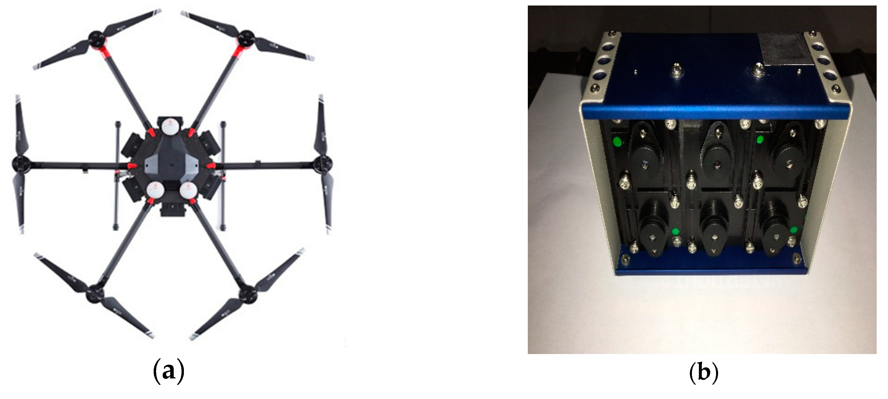
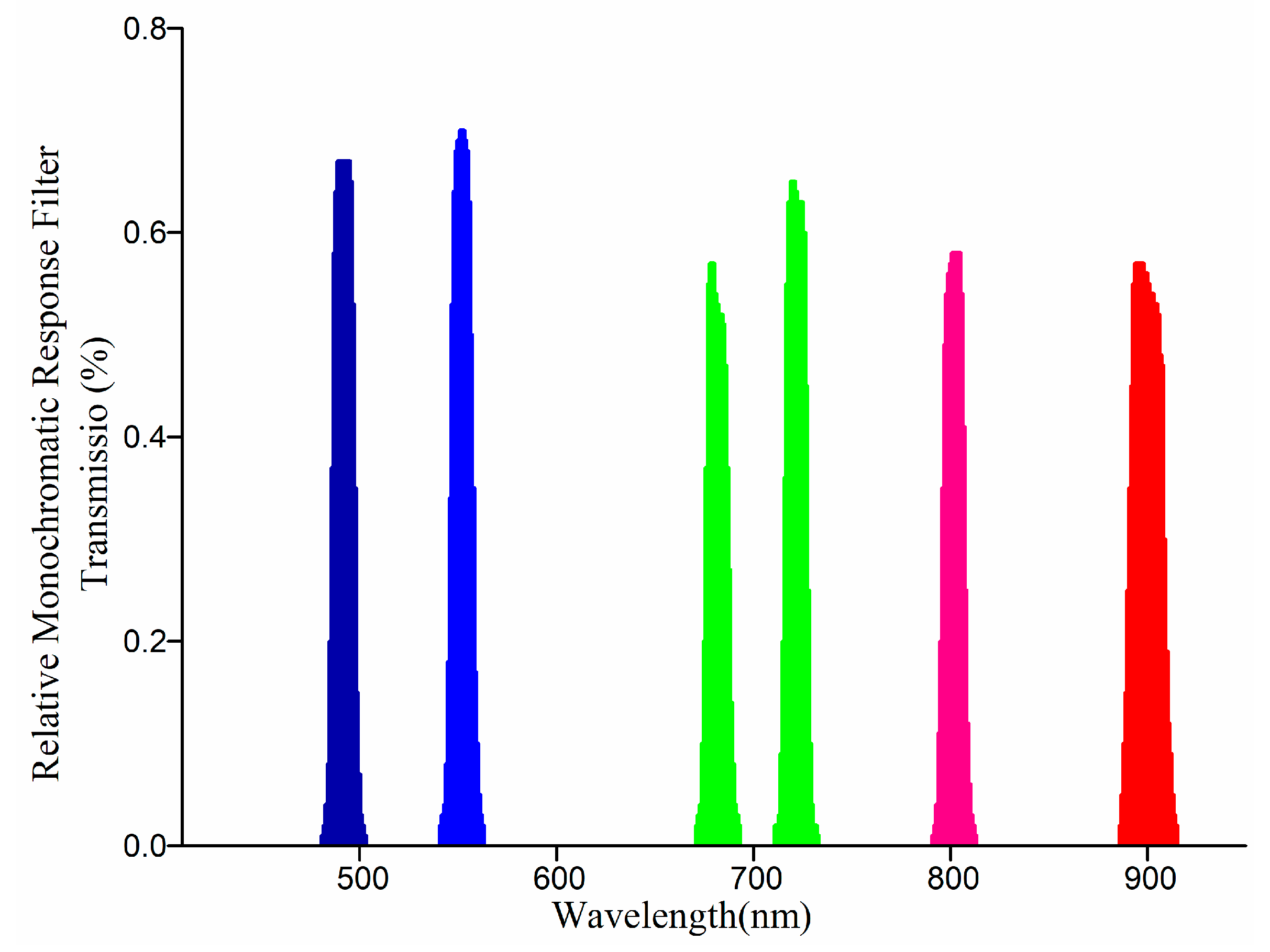
2.1. UAV, Sensors and Image Acquisition

The study area is located in a teaching experimental farm in Hebei (E115°50′, N39°20′), China (Figure 1). It is flat and typical agricultural farmland used for monitoring the growth of corn (May–August) and wheat (November–April). Figure 1a,b show detailed operations for calibration with homogeneous and heterogeneous targets for acquiring the multispectral images from different flight altitudes and varied weather conditions. The calibration targets are all customized, the reflectance is from 20%, 30%, 40%, and 60%, the reflectance is marked in Figure 1. In addition, two non-woven fabrics were also used, one white (reflectance of about 65%) and one black (reflectance of about 5%). In this study, the DJI M600 Pro UAV (Figure 2a) equipped with Mini MCA 6 multispectral camera (Figure 2b) were used as the data collection platform to acquire the multispectral images for monitoring agricultural growth.
The payload capacity of DJI M600 Pro is 15.5 kg, and the typical flight duration is 30 min depending on the payload size. The Mini MCA 6 is a product of Tetracam INC, which consists of six individual cameras arranged in 2 × 3 arrays. Each camera is equipped with a complementary metal oxide semiconductor (CMOS). Images can be acquired in forms of 8-bit or 10-bit and are stored in the memory cards.
The Mini MCA 6 has six spectroscopic filters for each camera, and the spectroscopic filters can allow a narrow band of wavelength to arrive at the spot on the camera, which means that the bands of this camera are all narrow bands (http://www.tetracam.com/Products-Micro_MCA.htm). The filters have a central wavelength of 490 (10), 550 (10), 680 (10), 720 (10), 800 (10), and 900 (20) nm. The detail of relationship between wavelength and relative monochromatic response filter transmission (%) and peak transmission wavelength of each filter is described in Figure 3.
The narrow bands can help to extract the sun-induced chlorophyll fluorescence, which has been a great potential indicator for predicting gross primary productivity [33]. Filters are interchangeable depending upon the purpose of UAV campaign. The flight mission is carefully planned with consideration of the position and attitude of the camera, the flight path, the image blocks, the overlaps between images, and the ground sampling distance (GSD) scale expressed in mm or cm [34]. The theoretical GSD value for the geometric resolution is given by,
GSD = Pixel   Size Focal   Length Distance   to   object
According to the Civil Aviation Safety Authority (CASA) laws, the flight altitude is restricted within three nautical miles of an aerodrome and a UAV is not allowed to operate above 120 m. To identify the effects of atmospheric attenuation, the spectral data is collected at different flight altitudes. Four flight heights flying altitude ranges from 25 to 100 m (25 m, 50 m, 75 m, and 100 m) and near-ground 1.5 m (by excluding the camera effects) were conducted on 7 June 2017 as shown in Figure 4. The camera was triggered automatically, and the data file with position, and attitude for each image was acquired. These images of different altitudes are single images.
Figure 5 clearly shows the three temporal images of the UAV covering the entire planted corn region which was operated on 7 June (sunny), 8 July (little cloud), and 14 August (more cloud) in 2017, to explore the inner effects of weather conditions on radiometric calibration.
The field data of ground control point (GCP) and analytical spectral device (ASD) data are collected during the flight durations. Each flight path is planned, established, and controlled using a processor mounted on the UAV platform. The flight speed of each flight is maintained around 7 m/s with 75% forward overlap as well as side overlap of images. Table 1 clearly shows the detail of data collection.

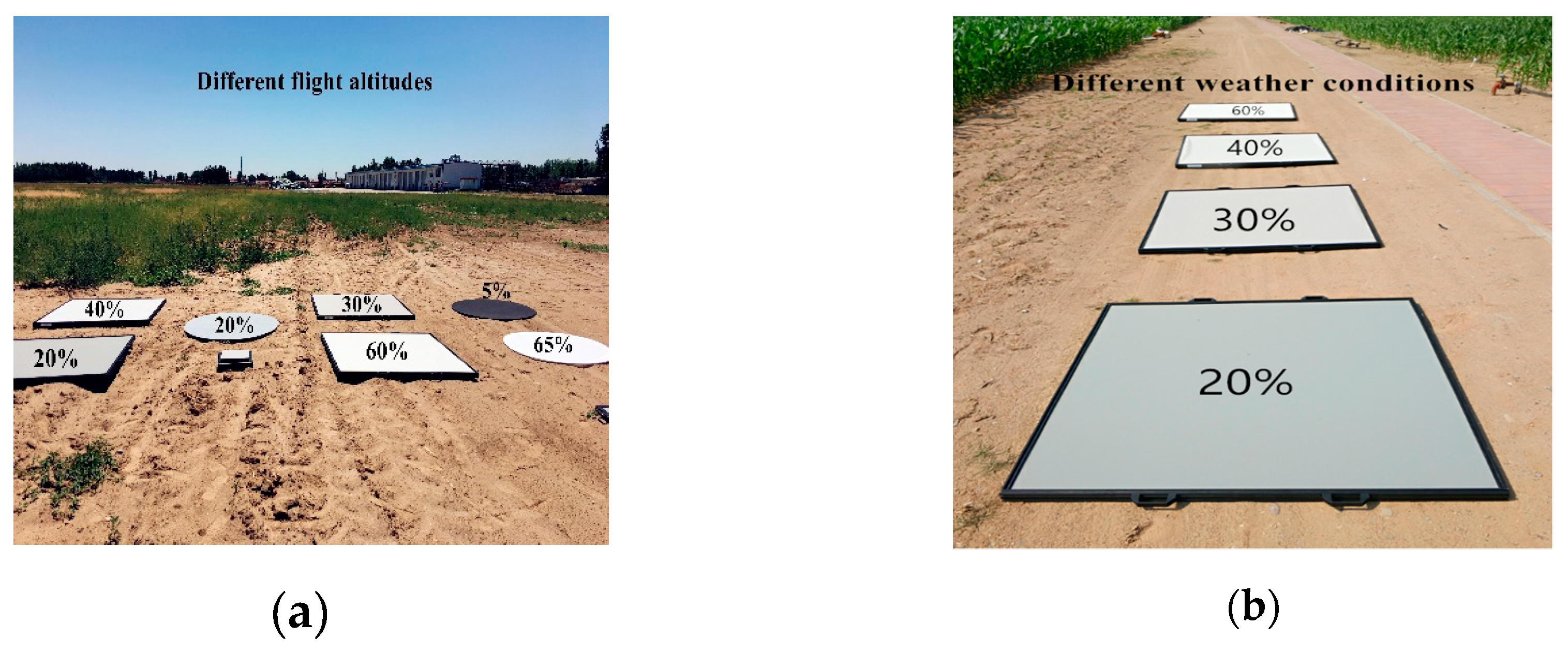
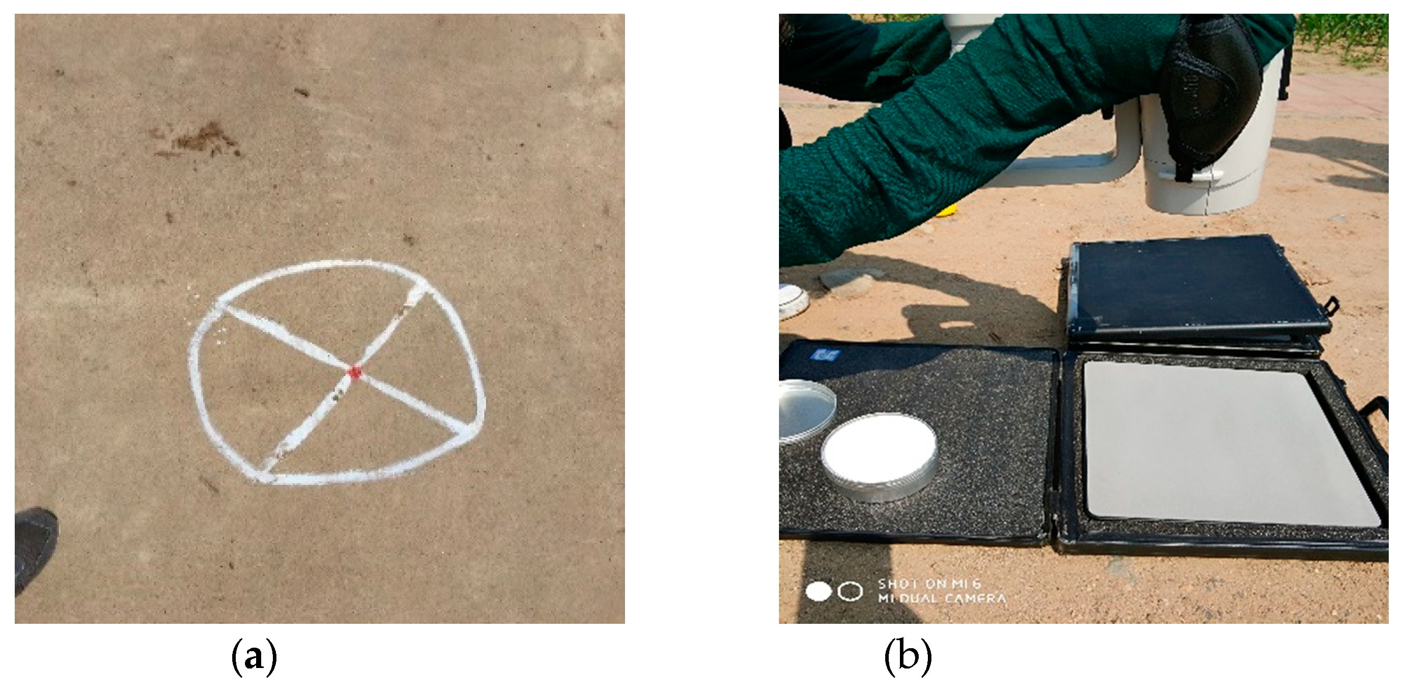
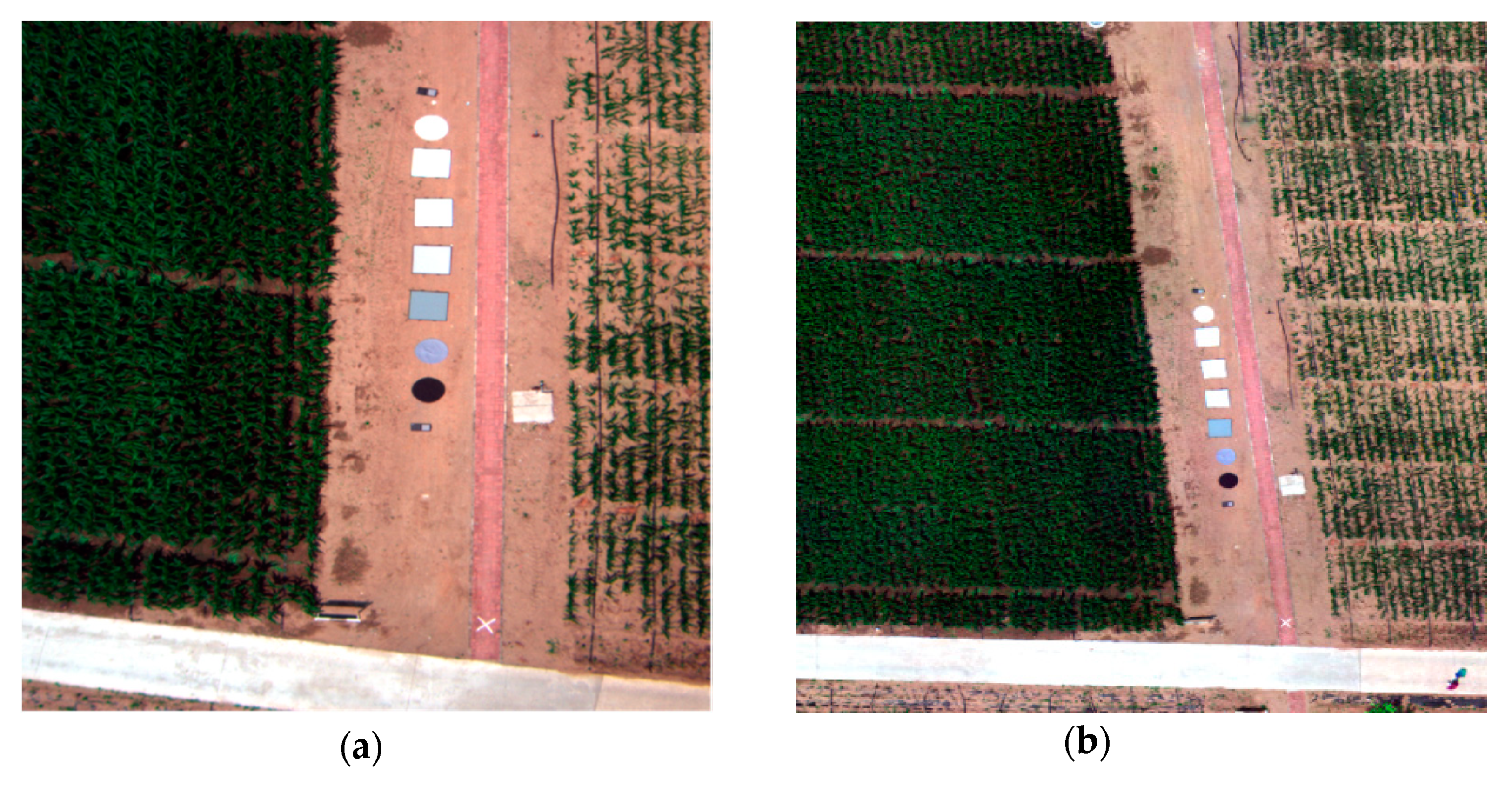
2.2. Ground Data Collection

GCPs are used to control the geometric accuracy of images [35]. In this study, the field data collection includes GCPs location and spectral measurement. The synchronous field data collection of GCP location and object spectrum spectral measurement are obtained using a Trimble real time kinematic (RTK) base station and an ASD handheld2 respectively. Six GCPs (Figure 6a) are made evenly spread across the whole area to control geometric distortion, the GCP locations are measured precisely by GPS, and the detail information is shown in Table 2. These GCP locations are fixed once the precise GPS information is confirmed.
Three pseudo targets (black 5%, gray 20%, and white 65%) and 4 professional radiometric calibration boards (20%, 30%, 40%, 60%) were used for radiometric calibration. All calibration targets were placed along the transect, and spectral measurements of each calibration target were taken by an ASD handheld2. This device works in a passive mode which can record the wavelength from 325 to 1075 nm. The handheld2 spectral radiometer is used in a variety of applications that require reflectance, transmittance, radiance, and irradiance measurements, and it is specially designed to acquire spectral measurements in the visible to a short-wave infrared range [8,26]. In this study, the reflectance measurements were taken during the flight campaign (11:30 am to 12:00 am) under different imaging weather conditions. Before each measurement, the handheld was corrected using the standard board shown in Figure 6b to obtain a much more precise result. The whole work of each spectral data collection was done ground control point within 10 min ground control point. The detailed information of radiometer calibration is shown in Figure 6b.

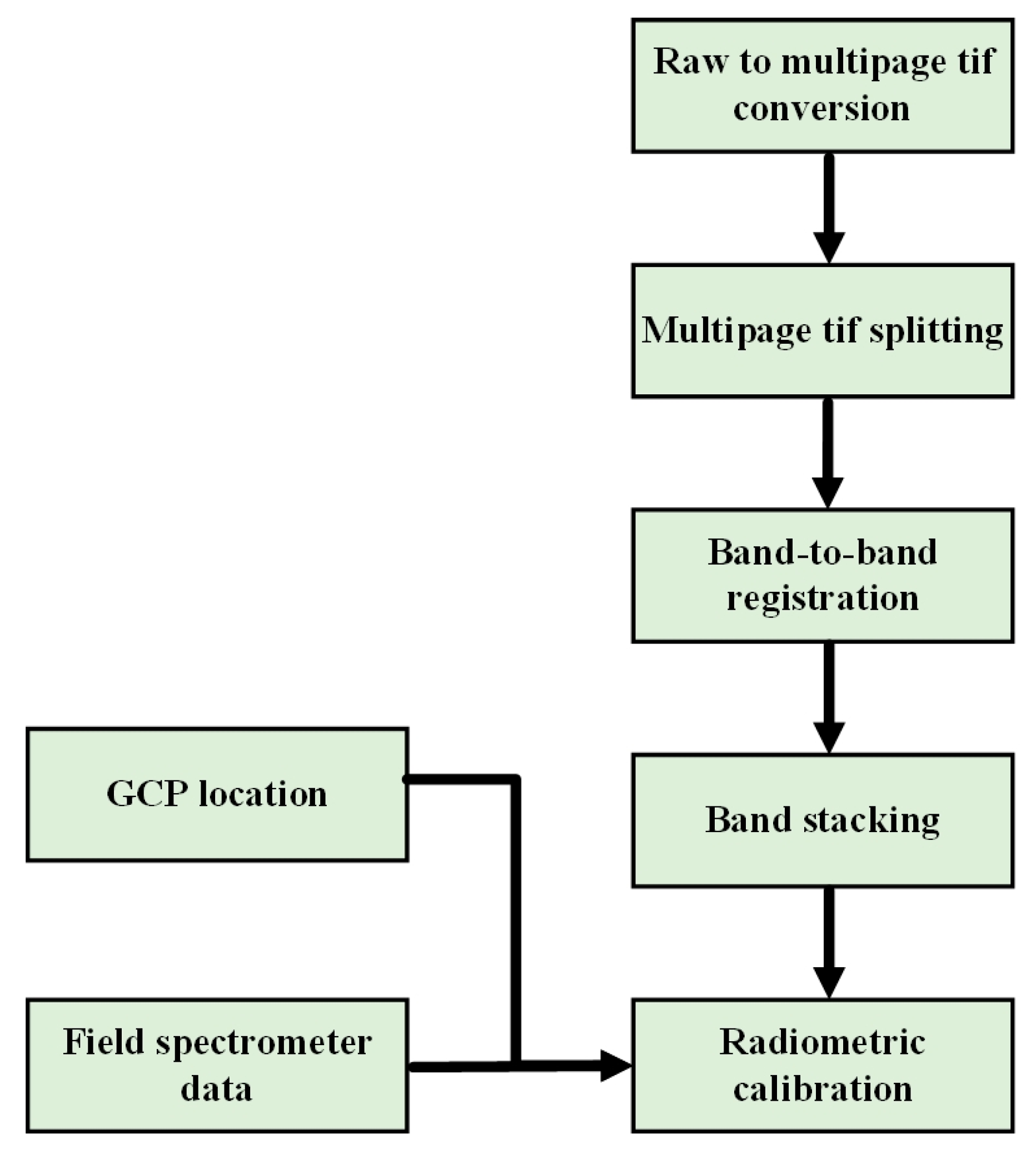
2.3. Data Processing
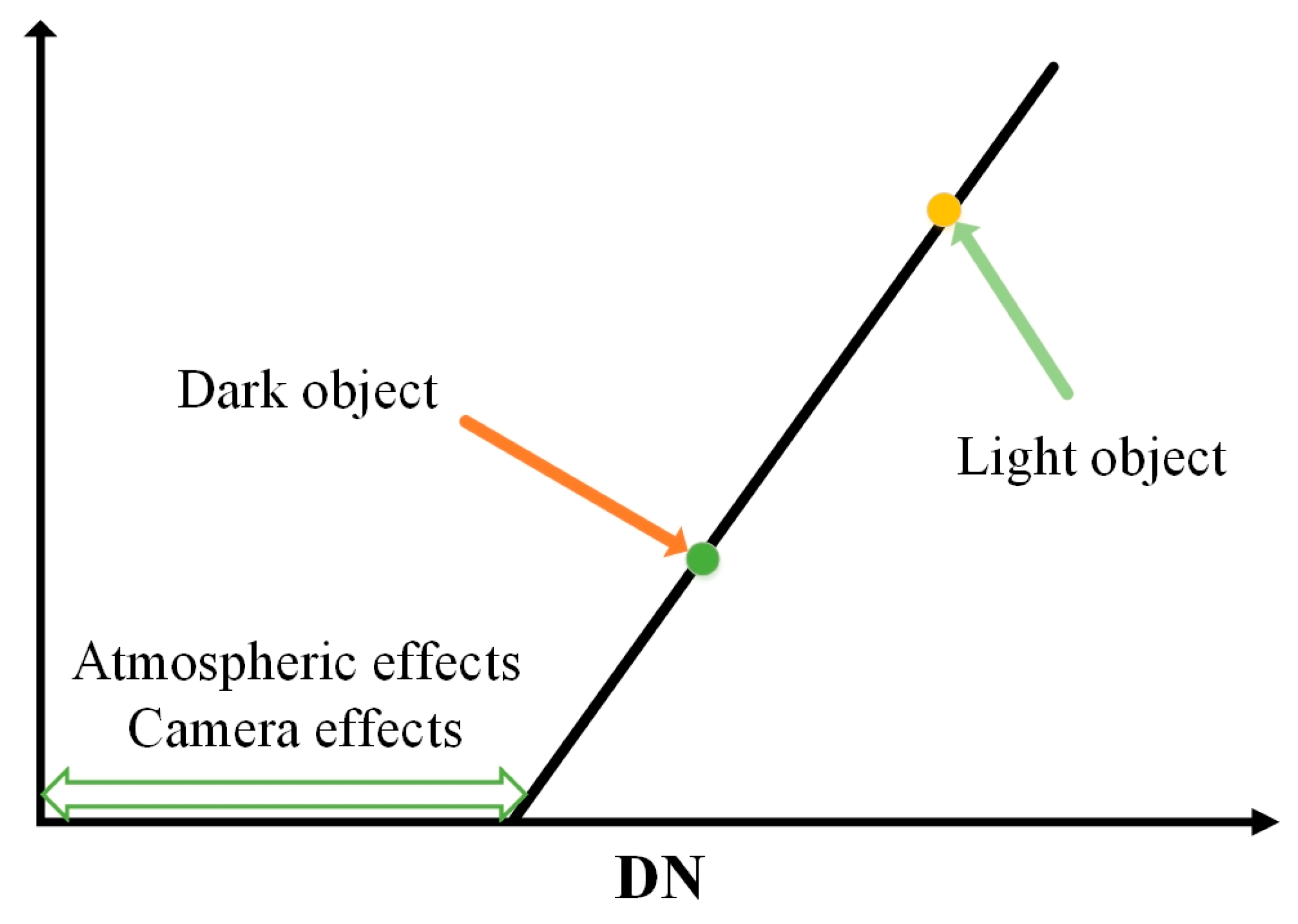
Figure 7 shows the data processing steps involved with the multispectral images acquired using a UAV platform. The raw data were then converted to multipage tif using PW2 provided by Tetracam INC. As the camera has six separate channels with each channel covering a different wavelength, the multipage TIFs each need to be geometrically registered to cover a six-band single multispectral image. The band-to-band registration of the images is crucial work to overcome the effect of spectral image analysis. The PW2 software is used for band-to-band registration of multipage tif that aligns considering the translation, rotation, and scaling between the reference and sensed images. This approach could only produce the registered images in relatively better alignment at the center of the image, where the BRDF effect and the lens falloff are believed to be relatively small. However, PW2 provides a convenient way of image alignment with high precision. In addition, the bit conversion is also performed using PW2 software.
Agisoft PhotoScan is a tool that performs photogrammetric processing of digital images and generates spatial data, 3D reconstruction, visualization surveying, and mapping tasks to be used in GIS and related applications. Agisoft PhotoScan is based on the structure from motion (SFM) technique and scale invariant feature transform (SIFT) operator. The GCP locations were used in Agisoft PhotoScan to control the plane accuracy, with all images being mosaiced in the software to generate the orthophoto images. The BRDF is not considered in this study, as it would possibly cost considerable time and the images and reflectance were all acquired in a nearly vertical form.
The ENVI 5.3 and Arcgis10.3 were used together to make regions of interest (ROIs), which were generated on pseudo calibration targets with a boxed buffer that could represent the real information of the energy. The selected ROIs contained the center of each pseudo calibration target, with commonly 50 or more pixels being covered. The DNs of each pseudo calibration target were extracted from multiple images.
Target reflectance was acquired over a Spectralon® panel. The Spectralon can calculate and record the radiance of objects. The Field Spec Pro acquires data in narrow bands that roughly at a resolution of 1 nm from wavelengths 350 to 2500 nm. As errors would not be possibly reduced if the near-continuous data is used directly, these data were averaged using the relative spectral response of each of the camera. The equation of resampling is given below [36].
R e f λ = λ 1 λ 2 R λ S λ d l λ 1 λ 2 S λ d l  
where λ1 and λ2 represent the start and stop wavelength of the channel respectively, Sλ refers to the spectral response of the channel at the wavelength, Rλ is the reflectance at the calibration plate of λ, Refλ is the equivalent reflectivity for the calculated channel.

2.4. Methodology

A linear regression based calibration is used to derive coefficients to fit the digital numbers of the MCA imagery to the field measured reflectance spectra. The LRM is adapted to a series of radiometric calibration of multispectral images acquired from different flight altitudes and varied weather conditions. This method has been widely used in the radiometric calibration of images acquired from satellites [37,38,39]. The reflectance spectrum of each of the calibration targets was measured on the ground with an ASD with the DNs of each band from the ROIs extracted from remotely sensed images [40,41]. The LRM assumes that the reflectance of targets from the ASD has a linear relationship with the DNs from each band of remotely sensed images as shown in Figure 8.
The line prediction equation is calculated for each band to predict surface reflectance from radiance using:
R = DN ∗ slope ± intercept
The above equation removes both illumination and atmospheric effects. The simplest approach is to use a single calibration target with the assumption that surfaces with zero reflectance will produce zero radiance at the sensor. The use of a single calibration target assumes that atmospheric scattering does not contribute to the radiance recorded by the sensor. By using more than two calibration targets, the relationship between the radiance recorded by the sensor and reflectance can be accurately determined. Hence, two or more calibration targets are suggested. The intercept of X-axis is DN ascribed to atmospheric radiance and camera noise. Therefore, once the camera noise is settled, the atmospheric radiance of different flight altitudes can be each obtained. In this study, the calibration was done by calculating the linear relationship between the DNs and reflectance for each band. Central pixels of a similar object were chosen to obtain an accurate relationship between the DN of UAV images and reflectance from the field measured data using ASD. The optimal number of calibration targets was confirmed for a single image from the sunny day, and then the calibration targets were used to calculate the intercepts of X-axis at different flight altitudes. Hence, the optimal calibration targets were considered to assess the atmospheric effects at different altitudes. A universal calibration equation was generated from the images acquired in the sunny weather conditions. Furthermore, this approach was used to calibrate the single image and mosaic images acquired from different weather conditions (sunny, little cloudy, and very cloudy).
Figure 9 shows the technique route of the proposed research. In the figure, three subsystems are shown considering different altitude and weather conditions and were used for images acquired using a multispectral camera mounted on a UAV. First, the different altitudes were useful to confirm the optimal calibration targets that can be used to reduce the camera and atmospheric effects. Second, based on the confirmed calibration targets, the mosaic effects were analyzed. Further, the proposed LRM method was tested on the mosaic images from different weather conditions with mosaic effects excluded. Third, based on the facts of the previous analyze; a universal equation for each band was proposed and tested.
The overall accuracy of the proposed method was assessed by comparing image-driven reflectance values with the field measured reflectance values. The calibration aims to obtain the reflectance of objects that are close to the reflectance from an ASD Handheld2. Therefore, the mean absolute deviation (indicated as V), root mean square error (RMSE) and normalized root mean square error (NRMSE) were adopted to assess the difference between the calibrated reflectance from multispectral images and original reflectance measured by an ASD Handheld2.
| v | = i = 1 n | y i x i | n
RMSE = i = 1 n ( y i x i ) 2 n
NRMSE = i = 1 n ( y i x i ) 2 n 100 n i n x i
where x i and y i each represent the reflectance from calibrated UAV images and field measurements, and n is the total number of calibration samples.

3. Results

In this section, the results of the proposed framework are discussed. The obtained results were evaluated for different weather conditions.

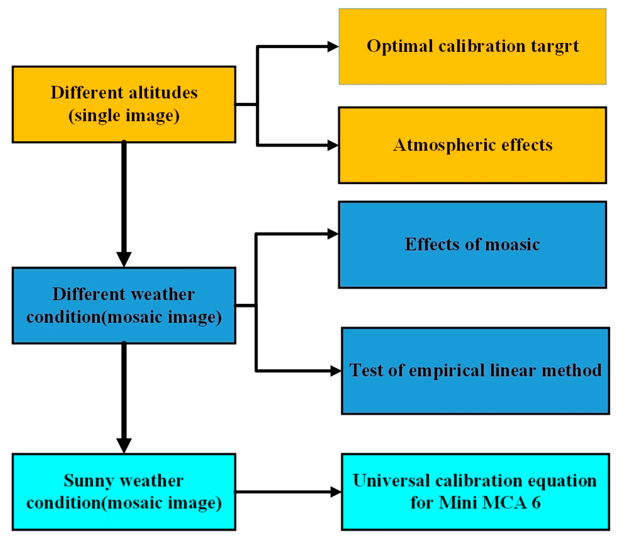
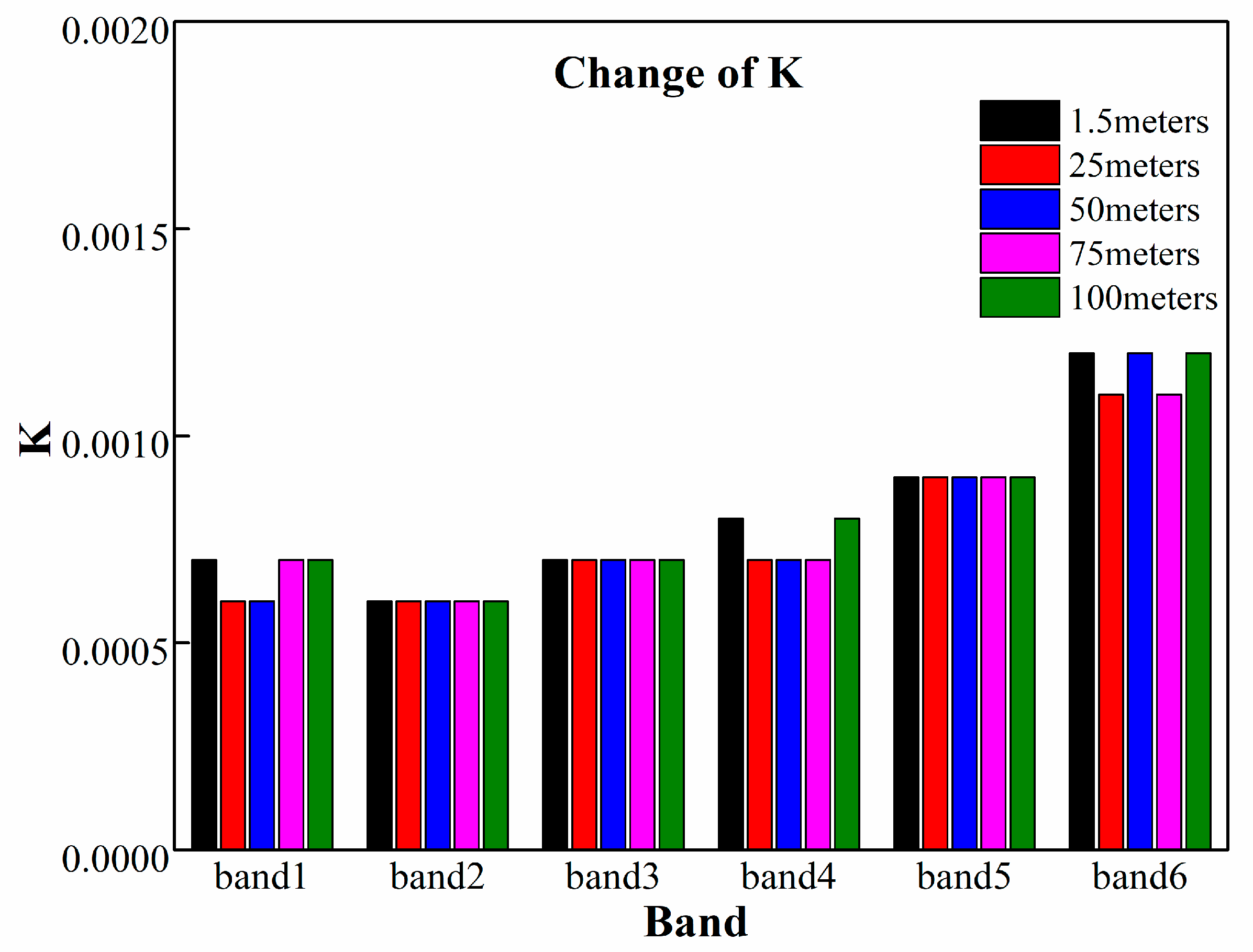
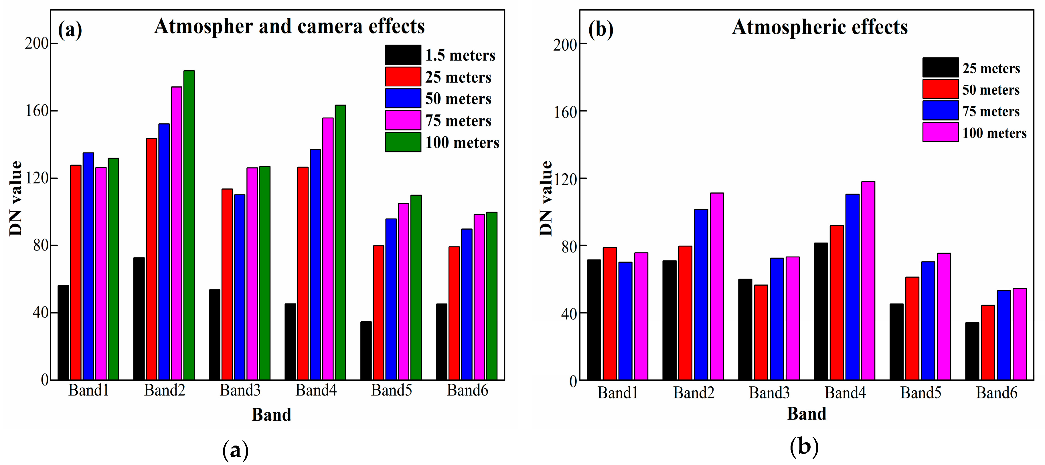
3.1. Single Images from Different Altitudes

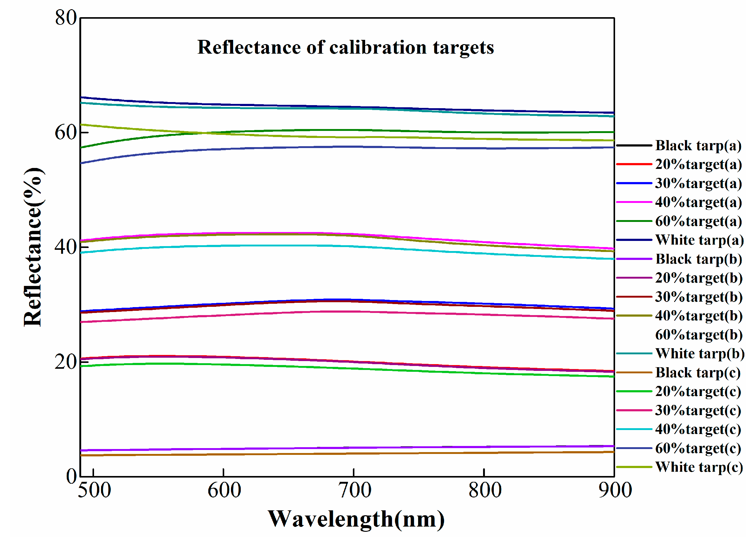
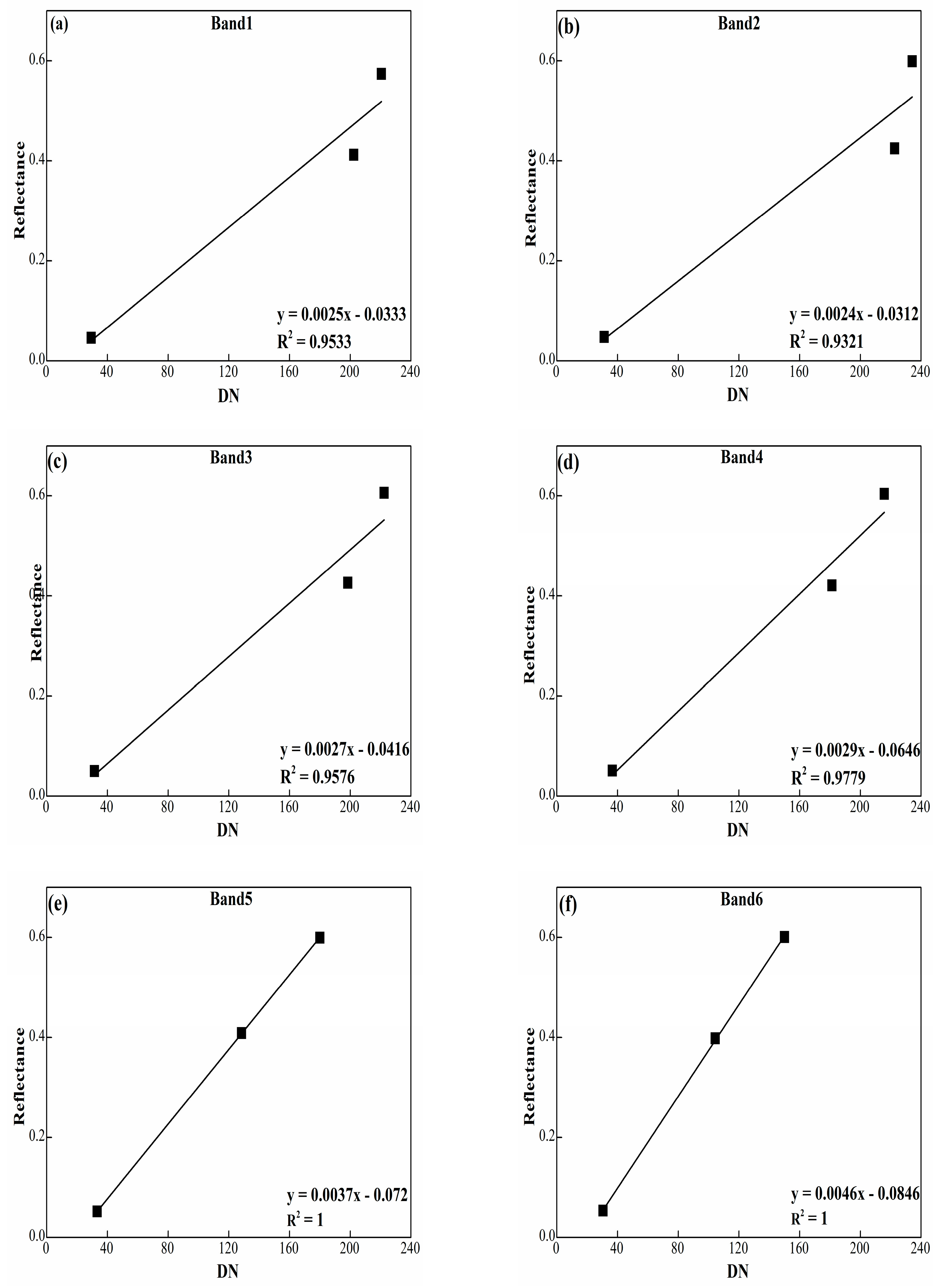
3.1.1. The Optimal Selection of Calibration Targets

First, the effects of a single image were evaluated at different flight altitudes. Among different flight heights, the UAV captured images to obtain the optimal selection of calibration targets. The number of calibration targets is changed, while the dark target and the white target are held constant settled as a black tarp (5% reflectance) and white calibration blank (60% reflectance), respectively. The measurement of reflectance was strictly performed as described in Section 2.4. The details of calibration targets are shown in Table 3. The number of calibration targets was added from two to five with changing combinations to confirm the optimal set of calibration targets.
The calibration results using the same validation targets and ROIs were adopted to exclude the errors while calculating. The results of V and RMSE using combination 1 were set as a base reference, the results of other combinations were compared with a base reference to make sure of the optimal combination. The results of combination 2, 3, and 4 using three calibration targets seem to have higher precision as the V and RMSE of these combinations were all less than those of combination 1. However, the V of combination 5, 6, 7, and 8 which used more numbers of calibration targets were all higher than the base reference. Only the RMSE of combination 6, 7, and 8 was less than that of the base reference. It can be obtained that the adoption of more targets may, to some extent, fit the LRM line well, especially for the adoption of three targets rather than two. But, when the number of targets continued to increase, the V and RMSE also increased. Using too many calibration targets may lead to lower accuracy, which may be ascribed to the random error of measurement from the instruments. In addition, the results will be better if the precision of the calibration can be maintained with the adoption of fewer calibration targets. The calibration targets are expensive, heavy, and hard to deploy in the field. Considering all issues, using only two or too many calibration targets is not advisable. Therefore, the optimal calibration combinations for Mini MCA 6 would probably be combination 2, 3, and 4. In other words, the optimal combination is supposed to include the dark object, moderate object, and white object. The main purpose of this study is to obtain the precisely calibrated images of corn growing at different stages and also band 1, band 2, band 3, and band 4 which are within the range of 400 nm to 760 nm. It is known that the reflectance of vegetation during this range of wavelength is under 15%. Therefore, the 20% target that is near 15% reflectance would be the best choice for this research. With all these matters considered, combination 2 using 5% target, 20% target, and 60% target is chosen as the most optimal combination, and it could be adopted for further analysis.

3.1.2. Atmospheric Effects

To obtain the atmospheric effects from different flight altitudes, the single images acquired from different altitudes were individually calibrated using LRM with the optimal calibration targets obtained in the previous section. The altitudes of four single image acquired from flight altitudes 25, 50, 75, and 100 m were individually calibrated and validated. With reference to the line fit using the LRM, the X-axis indicates the DN value of the multispectral camera with the atmospheric effects. Therefore, to obtain the precise atmospheric effects of images taken at different altitudes, the effects of the camera should be confirmed first. The camera effects were obtained by calibrating the images from 1.5 m above the ground on a farm within the same imaging environment. It was acquired in a similar environment and time to exclude the effects of uncertainty. Further, the atmospheric effects of four single images of multispectral data acquired at different altitudes were calculated by the difference between the intercept of X-axis. Table 4 shows the calibration equation of individual bands at different heights.
From Figure 10, it is clear that for each band, the constant K from band 1 to band 6 varied from 7.00E-4, 6.00E-4, 7.00E-4, 7.00E-4, 7.00E-4 to 1.20E-3 respectively. K represents the basic property of a camera. As K is stable for each band it means that this camera has a great potential for acquiring high quality images. The intercept is the changing variable, which has two aspects: camera effects (constant for each band) and atmospheric effects contributed to by the increase in flight altitudes. The camera effects can be acquired through the images from 1.5 m, and then the atmospheric effects can be acquired by X-axis minus the camera effects.
Using the optimal calibration targets, the calibration equation of each band for different altitudes were obtained. The intercept of 1.5 m (camera effects) and 25 to 100 m (atmospheric effects with and without camera effects) were calculated and are shown in Figure 11. From the figure, we can observe that the camera effects of each band are different, i.e., the DNs changes from 34 to 72. The atmospheric effects are two or three times more when compared with the camera effects. More importantly, the atmospheric effects would possibly influence the DN values even if the flight altitude is only 25 m, which would eventually lead to uncertainties in calculating vegetation indexes, such as NDVI and EVI.
To explore the impacts of these two factors on reflectance, the DNs were then put back into each specific calibration equation to obtain the effected reflectance. The effects of the camera to reflectance is about 0.0598%, the influence will be about 1% to the black tarp (5% reflectance). Table 5 shows the atmospheric effects of different flight altitudes. In this table, it can be observed that the atmospheric effects increase with an increase in flight altitudes. However, even if the altitude is 100 m the maximum will be around 1.5%. Therefore, the camera and atmospheric effects to reflectance can be reduced by acquiring multiple images in moderate low altitude (<100 m). The atmospheric effects vary with the altitudes and between the wavelengths (bands). Considering the image spatial resolution and acquiring effectiveness, the altitude of 50 m is suggested for agricultural and ecological applications using multispectral images. Thus, multispectral images have the advantage in the temporal collection of data.

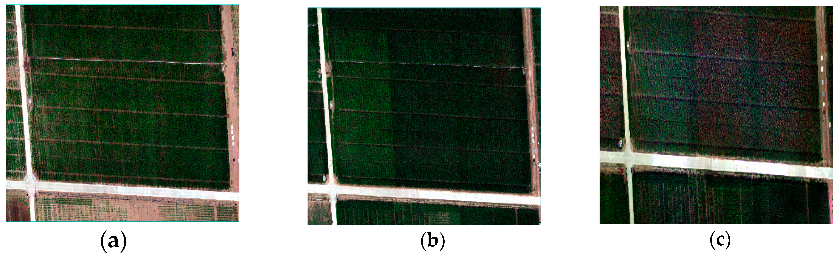
3.2. Mosaic Images of Different Weather Conditions

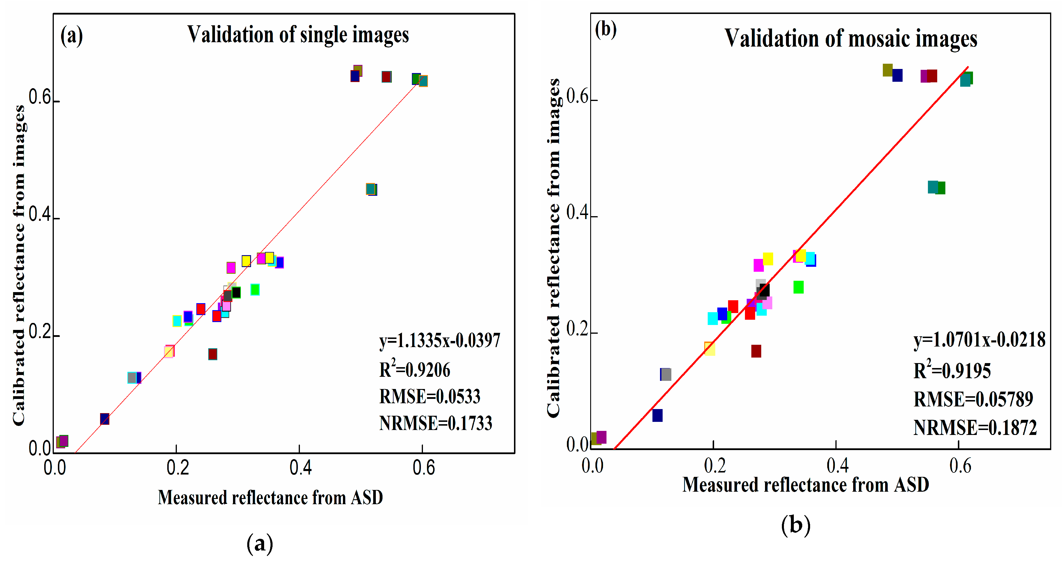
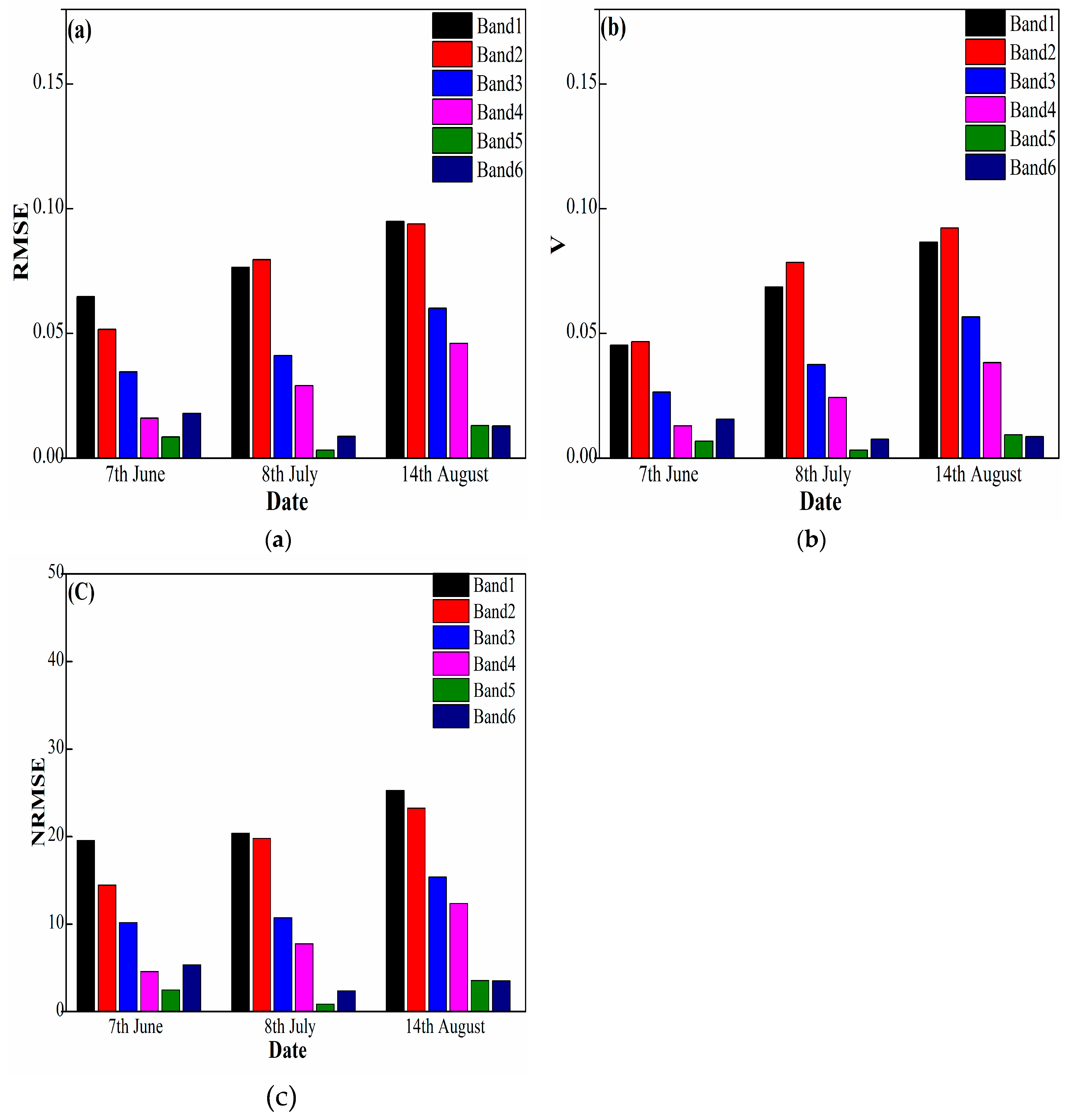
3.2.1. Effects of Mosaic to Radiometric Calibration

When file conversion and band-to-band registration were applied in PW2 software, some corrections, such as anisotropic effects, need to be handled. However, some vignetting effects remained. The registered images were mosaicked using Photoscan software. These images were processed by the white balance and histogram equalization to make the whole image pixel distribution alike. By doing the above steps, the DNs of the images of each band are changed. To assess the effects using the above processing steps, there is a need to explore the change in DN values.
To explore the effects of mosaic, the single image and mosaic image (Figure 12) covering the whole radiometric targets were selected from the images which were acquired during daytime on 7 June 2017.
To make par comparison, the ROIs covering the same region were selected in the images (single image and mosaic image). The calibration equations for a single image and mosaic image are shown in Table 6.
From Figure 13, the RMSE of a single image and mosaic image assessed are 0.533 and 0.578 respectively. The normalized RMSE was also calculated, the NRMSE for a single image and mosaic image were 0.1733 and 0.1873, respectively. However, the RMSE and NRMSE of mosaic image were a little larger than the single image; the error has possibly resulted from the effects of illumination, or the vignetting. Considering the calibration of multiple images based on the efficiency and effectiveness, calibration of a mosaic is much easier and timesaving than applying the calibration to each of multiple single images. Therefore, the mosaic image of a whole study area is suggested for calibrations.

3.2.2. Test of Linear Regression Method in Different Weather Conditions

We know that sunshine will certainly influence the radiation; therefore, the images taken from different weather conditions are different as well. To explore the effects of weather condition on calibration, the images are acquired on 7 June, 8 July, and 14 August 2017. Seven June was sunny with no wind, 8 July was with a little cloudy, and 14 August 2017 had more cloud.
Professional instruments for observing the weather are very expensive and not so easy to use in the field. To analyze the differences in weather conditions, the reflectance of the black tarp, white trap, and calibration targets acquired during three different weather condition were measured from an ASD and resampled to obtain the difference. Figure 14 clearly shows that the reflectance of the same target is different in different weather conditions; commonly the reflectance measured on a sunny day is larger than the reflectance measured on a cloudy day.
The reflectance of the black trap measured on a sunny day on 7 June is regarded as the reference reflectance, and then the relative changes of reflectance are calculated through the equations below:
| ASD 7.8 ASD 6.7 | ASD 6.7 100 %
| ASD 8.14 ASD 6.7 | ASD 6.7 100 %
The ASD reflectance from 8 July is approximate 1.5% lower than 7 June, and 14 August is about 6% lower than 7 June. To explore the common use of the LRM in different weather conditions, the images in three different weather conditions were calibrated and validated precisely. The images acquisition time and the selected locations and areas of calibration targets are held constant. In other words, the only change variable is the weather condition.
The images acquired from these three days of different weather conditions were individually calibrated and validated. The radiometric calibration was done using the LRM with the selected ROIs and the validation targets to be the same. The only change is the reflectance obtained from different weather condition. The highest V and RMSE of three days were 0.07 and 0.05, respectively. Therefore, the LRM with the real-time ASD reflectance can acquire high precision in calibration even during cloudy weather.

3.3. Universal Calibration Equation for Mini MCA 6

During a series of calibrations, it can be obtained that the calibration equations of Mini MCA 6 multispectral camera are very much alike. Therefore, we considered if one universal calibration equation could be proposed and could be used for Mini MCA 6 camera calibration with images acquired in a similar imaging environment as that of 7 June. To test this concept, the multispectral images acquired from a sunny day on 7 June were carefully calibrated to obtain the calibration equation. The detail information of the relationship R2 between DN and reflectance is shown in Figure 15. The universal calibration equations for each band is also shown in the figure.
The universal calibration equation was used to calibrate the multispectral images acquired on 8 July (little cloudy), and 14 August (more cloud). Then all these three calibrated images were converted to reflectance images, the reflectance of ROIs from images was compared with the reflectance from resampled reflectance from an ASD Handheld-2. The performance of indicators V, RMSE and NRMSE were used to assess the precision of calibration.
Figure 16 shows that the calibration results of images acquired on 7 June (sunny) and 8 July (little cloudy) using universal calibration equation, the results show that calibrated reflectance and validated target are very close. Commonly, the fifth and sixth band are calibrated much more precisely when compared with the other four bands. This is mainly due to the wavelength of the fifth and six are 800 nm and 900 nm respectively, which have more energy absorption than the other scale of the wavelength used in the camera. The V and RMSE for 7 June (sunny) and 8 July (little cloud) are all less than 7%. Hence, the universal calibration equation we proposed for Mini MCA 6 camera can be performed well to calibrate the radiance images to reflectance images. However, the universal calibration equation may not be suitable for calibrating the image data acquired on 14 August (more cloud). The V and RMSE are commonly larger than the other two days, especially the band 2 that has passed over 9% for V and RMSE. In general, we have enough reason to justify that in a similar weather condition, and altitudes, the proposed universal calibration equations for each band of the camera will radiometrically calibrate with the Mini MCA 6 camera.

4. Discussion

In agricultural and ecological related applications using the multispectral images acquired from low altitudes of a UAV platform, the camera effects and atmospheric correction are always neglected and are merely mentioned. Before our research, some applications just mentioned that their images were calibrated into reflectance with the precision of calibration unknown, commonly, with no or little professional calibration targets. Furthermore, some studies have involved calibrations using a laboratory calibration method, which is quite difficult to perform in field calibrations.
In this research, a quick and precise radiometric calibration method was proposed and adopted. To exclude the errors from Lambertian effects, the linear Lambertian calibration targets were adopted. In previous studies, the usage of calibration targets is not set. The adoption of calibration targets is an uncertainty due to different applications and scenes. In agricultural and ecological applications, the common study object is vegetation. The reflectance would possibly change with the wavelength. However, related researches were only conducted in satellite-based images. Therefore, we need to know how the selection of calibration targets influences the calibration results. In UAV-based applications, an optimal combination use of multi calibration targets was confirmed in agricultural applications.
The atmospheric effects were commonly neglected due to the little impacts. However, the real effects to the calibrations are unknown. Therefore, we assessed the atmospheric effects caused by cloud by assessing the calibration results from different flight altitudes. We have found that the atmospheric effects within 100 m of flight altitudes only contributes a little to the DN values. And from Figure 11, it can be obtained that the effects to different bands are totally different, the results show overall the effects are decreasing from band 1 to band 6. This is likely because the longer the wavelength, the more power the wavelength would possibly contain. In total, as the atmospheric effects are quite small, they can be neglected as the precision is already satisfactory in agricultural and ecological related calibrations.
Images from different weather conditions were merely mentioned in previous studies. So far, we do not know if the images can be used for further research from bad weather conditions, such as cloud. The apparent reflectance will be different for the same object in different weather conditions. We want to find out the effects of different weather conditions, and how much it will influence the radiometric calibration. We applied the radiometric calibration with the same method, calibration and validation targets. The calibration results of a sunny day and with little cloud indicate that the calibrated reflectance could be used for further research. While for the day with more cloud, we found that we cannot use the images from this weather condition, because the reflectance measured from an ASD showed a 20% decline compared with reflectance acquired on a sunny day.
So far, there has never been a universal calibration equation for this camera. Therefore, a universal calibration equation should be given and assessed. The results show that a universal calibration equation could be well used in similar imaging conditions. It is quite satisfactory to perform radiometric calibration in agricultural and ecological applications. For example, if a series of experiments conducted over a few days and in similar weather conditions and imaging environment, the acquisition of reflectance from the calibration targets might be reduced, which is a real problem in field data collection. The adoption of this universal calibration equation has proposed an innovative idea for quick radiometric calibration, meanwhile, saving much time and human power.
Even though the series of radiometric calibration were conducted under a strict procedure, there are also uncertainties from three main approaches: (1) linear regression method, (2) error from ASD, (3) Lambertian properties of the calibration target. First, the DN values are considered to have a linear relationship with reflectance measured from the same ROI in the LRM. However, the linear relationship is not always true for all circumstances. In this study, the precision of radiometric calibration is very high. Therefore, the DN and reflectance have a linear relationship within Mini MCA 6 camera with professional calibration targets. Future studies should explore the relationship between DN value and reflectance with infrared and near-infrared bands, which seems to have a quadratic or index relationship. Second, the error from ASD can be divided into two aspects: measurement error and resample error. Even though the Handheld2 is a professional instrument which can be used to record the spectral properties of objects, the instrument still has some limitations, such as, before each measurement the calibration should be strictly performed for the Handheld2. To keep it on par with the sunlight, the calibration is commonly done every five minutes. Therefore, there are uncertainties in this. Moreover, the spectral response function is only an approximate representation of the response of the camera to each wavelength. Third, the Lambertian properties of the calibration target will also influence the results, making the results less reliable. Therefore, to explore the effects of Lambertian properties, the BRDF correction should be considered in future experiments.

5. Conclusions

This paper describes a radiometric calibration technique using the linear regression method for calibrating images acquired by a Mini MCA 6 sensor mounted on a UAV platform. The images are acquired in two forms: single images and mosaic images and are acquired from different altitudes and in different weather conditions. A list of useful conclusions is observed from the series of radiometric calibration.
First, for the experiment of single images acquired from different flight altitudes, two main aspects were assessed: the optimal selection of calibration targets, and atmospheric effects. The results show that three calibration targets containing dark, moderate, and white calibration targets are possibly the best for the radiometric calibration of the Mini MCA 6 sensor. In addition, the atmospheric effects grow with an increase in flight altitude. However, the effects under 100 m are moderately low (1.5%) compared with the reflectance of ground calibration targets. Therefore, the atmospheric effects on a sunny day will have little effect. With the effectiveness of acquiring images and spatial resolution, a flight altitude of 50 m is suggested.
Second, another experiment was conducted using the mosaic images acquired on three days of different weather conditions. The RMSE of mosaic effects was 0.057 in comparison to single image effects of 0.053. The result indicates that the effects of the mosaic are little enough to not be considered when applying calibrations. Through the exclude of effects of mosaic, the mosaic images were each calibrated using the images and measured calibration targets reflectance from the same day. The LRM was successfully used to calibrate the images acquired from a sunny day, a little cloudy day, and cloudier day.
Third, a universal calibration equation for Mini MCA 6 was obtained from a sunny day and then validated using multispectral images from little cloudy and more cloud. The results show that in low flight altitudes, the universal calibration equation for Mini MCA 6 can be applied, and has obtained high precision calibration during a sunny day and a little cloud day. This study provides a standard procedure for acquiring and calibrating multispectral images in agricultural and ecological applications.

Author Contributions

Conceptualization, Y.G.; Data curation, Y.G.; Formal analysis, Y.G.; Investigation, Y.G.; Methodology, Y.G.; Software, Y.G., Z.Z. and H.H.; Supervision, W.W.; Validation, Y.G.; Visualization, Y.G.; Writing—original draft, Y.G.; Writing—review & editing, J.S., W.W. and X.Z.

Funding

This research was funded by the Strategic Priority Research Program of the Chinese Academy of Sciences (XDA19040304) and the National Key Research and Development Program of China Grants (Grant No. 2016YFA0602402).

Acknowledgments

The authors are grateful to Francisco Agüera-Vega and Pablo Zarco-Tejada.

Conflicts of Interest

The authors declare no conflict of interest.

References

  1. Laliberte, A.S.; Goforth, M.A.; Steele, C.M.; Rango, A. Multispectral Remote Sensing from Unmanned Aircraft: Image Processing Workflows and Applications for Rangeland Environments. Remote Sens. 2011, 3, 2529–2551. [Google Scholar] [CrossRef] [Green Version]
  2. Jhan, J.-P.; Rau, J.-Y.; Huang, C.-Y. Band-to-band registration and ortho-rectification of multilens/multispectral imagery: A case study of MiniMCA-12 acquired by a fixed-wing UAS. Isprs J. Photogramm. Remote Sens. 2016, 114, 66–77. [Google Scholar] [CrossRef]
  3. Mulla, D.J. Twenty five years of remote sensing in precision agriculture: Key advances and remaining knowledge gaps. Biosyst. Eng. 2013, 114, 358–371. [Google Scholar] [CrossRef]
  4. Hamylton, S.; Hedley, J.; Beaman, R. Derivation of High-Resolution Bathymetry from Multispectral Satellite Imagery: A Comparison of Empirical and Optimisation Methods through Geographical Error Analysis. Remote Sens. 2015, 7, 16257–16273. [Google Scholar] [CrossRef]
  5. He, Y.; Bo, Y.; Chai, L.; Liu, X.; Li, A. Linking in situ LAI and fine resolution remote sensing data to map reference LAI over cropland and grassland using geostatistical regression method. Int. J. Appl. Earth Obs. Geoinf. 2016, 50, 26–38. [Google Scholar] [CrossRef]
  6. Choudhury, B.J.; Tucker, C.J. Monitoring global vegetation using Nimbus-7 37 GHz Data Some empirical relations. Int. J. Remote Sens. 1987, 8, 1085–1090. [Google Scholar] [CrossRef]
  7. Duan, T.; Chapman, S.C.; Guo, Y.; Zheng, B. Dynamic monitoring of NDVI in wheat agronomy and breeding trials using an unmanned aerial vehicle. Field Crop. Res. 2017, 210, 71–80. [Google Scholar] [CrossRef]
  8. Grebby, S.; Cunningham, D.; Tansey, K.; Naden, J. The Impact of Vegetation on Lithological Mapping Using Airborne Multispectral Data: A Case Study for the North Troodos Region, Cyprus. Remote Sens. 2014, 6, 10860–10887. [Google Scholar] [CrossRef] [Green Version]
  9. Zhang, X.; Jayavelu, S.; Liu, L.; Friedl, M.A.; Henebry, G.M.; Yan, L.; Schaaf, C.B.; Richardson, A.D.; Gray, J. Evaluation of land surface phenology from VIIRS data using time series of PhenoCam imagery. Agric. For. Meteorol. 2018, 256, 137–149. [Google Scholar] [CrossRef]
  10. Honkavaara, E.; Arbiol, R.; Markelin, L.; Martinez, L.; Cramer, M.; Bovet, S.; Chandelier, L.; Ilves, R.; Klonus, S.; Marshal, P.; et al. Digital Airborne Photogrammetry—A New Tool for Quantitative Remote Sensing?—A State-of-the-Art Review On Radiometric Aspects of Digital Photogrammetric Images. Remote Sens. 2009, 1, 577–605. [Google Scholar] [CrossRef] [Green Version]
  11. Berk, A.; Anderson, G.P.; Acharya, P.K.; Dothe, H.; AdlerGolden, S.M.; Richtsmeier, S.C.; Hoke, M.L. MODTRAN4 radiative transfer modeling for atmospheric correction. Int. Soc. Opt. Photonics 1999, 3756, 348–353. [Google Scholar]
  12. Anderson, G.P.; Berk, A.; Acharya, P.K.; Dothe, H.; Adlergolden, S.M.; Ratkowski, A.J.; Felde, G.W.; Gardner, J.A.; Hoke, M.L.; Richtsmeier, S.C. Algorithms for Multispectral, Hyperspectral, and Ultraspectral Imagery VI, 2000. In MODTRAN4: Radiative Transfer Modeling for Remote Sensing; SPIE: San Jose, CA, USA, 2000. [Google Scholar]
  13. Vermote, E.F.; Tanre, D.; Deuze, J.L.; Herman, M. Second Simulation of the Satellite Signal in the Solar Spectrum, 6S: An overview. Geosci. Remote Sens. IEEE Trans. 2002, 35, 675–686. [Google Scholar] [CrossRef]
  14. Wu, J.; Wang, D.; Bauer, M.E. Image-based atmospheric correction of QuickBird imagery of Minnesota cropland. Remote Sens. Environ. 2005, 99, 315–325. [Google Scholar] [CrossRef]
  15. Mishra, V.D.; Sharma, J.K.; Singh, K.K.; Thakur, N.K.; Kumar, M. Assessment of different topographic corrections in AWiFS satellite imagery of Himalaya terrain. J. Earth Syst. Sci. 2009, 118, 11–26. [Google Scholar] [CrossRef] [Green Version]
  16. Richter, R. A spatially adaptive fast atmospheric correction algorithm. Int. J. Remote Sens. 1996, 17, 1201–1214. [Google Scholar] [CrossRef]
  17. Liang, S. Quantitative Remote Sensing of Land Surfaces; Wiley-Interscience: Hoboken, NJ, USA, 2004; pp. 413–415. [Google Scholar]
  18. Thome, K.J. Absolute radiometric calibration of Landsat 7 ETM+ using the reflectance-based method. Remote Sens. Environ. 2001, 78, 27–38. [Google Scholar] [CrossRef]
  19. Ahmed, O.S.; Shemrock, A.; Chabot, D.; Dillon, C.; Williams, G.; Wasson, R.; Franklin, S.E. Hierarchical land cover and vegetation classification using multispectral data acquired from an unmanned aerial vehicle. Int. J. Remote Sens. 2017, 38, 2037–2052. [Google Scholar] [CrossRef]
  20. Akar, A.; Gökalp, E.; Akar, Ö.; Yılmaz, V. Improving classification accuracy of spectrally similar land covers in the rangeland and plateau areas with a combination of WorldView-2 and UAV images. Geocarto Int. 2016, 32, 990–1003. [Google Scholar] [CrossRef]
  21. Vega, F.A.; Ramírez, F.C.; Saiz, M.P.; Rosúa, F.O. Multi-temporal imaging using an unmanned aerial vehicle for monitoring a sunflower crop. Biosyst. Eng. 2015, 132, 19–27. [Google Scholar] [CrossRef] [Green Version]
  22. Bagheri, N. Development of a high-resolution aerial remote-sensing system for precision agriculture. Int. J. Remote Sens. 2016, 38, 2053–2065. [Google Scholar] [CrossRef]
  23. Garciaruiz, F.; Sankaran, S.; Maja, J.M.; Lee, W.S.; Rasmussen, J.; Ehsani, R. Comparison of two aerial imaging platforms for identification of Huanglongbing-infected citrus trees. Comput. Electron. Agric. 2013, 91, 106–115. [Google Scholar] [CrossRef]
  24. Candiago, S.; Remondino, F.; De Giglio, M.; Dubbini, M.; Gattelli, M. Evaluating Multispectral Images and Vegetation Indices for Precision Farming Applications from UAV Images. Remote Sens. 2015, 7, 4026–4047. [Google Scholar] [CrossRef] [Green Version]
  25. Primicerio, J.; Gennaro, S.F.D.; Fiorillo, E.; Genesio, L.; Lugato, E.; Matese, A.; Vaccari, F.P. A flexible unmanned aerial vehicle for precision agriculture. Precis. Agric. 2012, 13, 517–523. [Google Scholar] [CrossRef]
  26. Del Pozo, S.; Rodríguez-Gonzálvez, P.; Hernández-López, D.; Felipe-García, B. Vicarious Radiometric Calibration of a Multispectral Camera on Board an Unmanned Aerial System. Remote Sens. 2014, 6, 1918–1937. [Google Scholar] [CrossRef] [Green Version]
  27. Senthilnath, J.; Kandukuri, M.; Dokania, A.; Ramesh, K.N. Application of UAV imaging platform for vegetation analysis based on spectral-spatial methods. Comput. Electron. Agric. 2017, 140, 8–24. [Google Scholar] [CrossRef]
  28. Song, L.; Guanter, L.; Guan, K.; You, L.; Huete, A.; Ju, W.; Zhang, Y. Satellite sun-induced chlorophyll fluorescence detects early response of winter wheat to heat stress in the Indian Indo-Gangetic Plains. Glob. Chang. Biol. 2018, 24, 4023–4037. [Google Scholar] [CrossRef] [PubMed]
  29. Damm, A.; Guanter, L.; Paul-Limoges, E.; Tol, C.V.D.; Hueni, A.; Buchmann, N.; Eugster, W.; Ammann, C.; Schaepman, M.E. Far-red sun-induced chlorophyll fluorescence shows ecosystem-specific relationships to gross primary production: An assessment based on observational and modeling approaches. Remote Sens. Environ. 2015, 166, 91–105. [Google Scholar] [CrossRef]
  30. Gitelson, A.A.; Peng, Y.; Arkebauer, T.J.; Schepers, J. Relationships between gross primary production, green LAI, and canopy chlorophyll content in maize: Implications for remote sensing of primary production. Remote Sens. Environ. 2014, 144, 65–72. [Google Scholar] [CrossRef]
  31. Berni, J.A.J.; Zarco-Tejada, P.J.; Suarez, L.; Fereres, E. Thermal and Narrowband Multispectral Remote Sensing for Vegetation Monitoring From an Unmanned Aerial Vehicle. Ieee Trans. Geosci. Remote Sens. 2009, 47, 722–738. [Google Scholar] [CrossRef] [Green Version]
  32. Myneni, R.B.; Hoffman, S.; Knyazikhin, Y.; Privette, J.L.; Glassy, J.; Tian, Y.; Wang, Y.; Song, X.; Zhang, Y.; Smith, G.R. Global products of vegetation leaf area and fraction absorbed PAR from year one of MODIS data. Remote Sens. Environ. 2002, 83, 214–231. [Google Scholar] [CrossRef] [Green Version]
  33. Duveiller, G.; Cescatti, A. Spatially downscaling sun-induced chlorophyll fluorescence leads to an improved temporal correlation with gross primary productivity. Remote Sens. Environ. 2016, 182, 72–89. [Google Scholar] [CrossRef] [Green Version]
  34. Sutton, A.; Fidan, B.; Walle, D.V.D. Hierarchical UAV Formation Control for Cooperative Surveillance. Ifac Proc. Vol. 2008, 41, 12087–12092. [Google Scholar] [CrossRef]
  35. Harwin, S.; Lucieer, A. Assessing the Accuracy of Georeferenced Point Clouds Produced via Multi-View Stereopsis from Unmanned Aerial Vehicle (UAV) Imagery. Remote Sens. 2012, 4, 1573–1599. [Google Scholar] [CrossRef] [Green Version]
  36. Dinguirard, M.; Slater, P.N. Calibration of Space-Multispectral Imaging Sensors: A Review. Remote Sens. Environ. 1999, 68, 194–205. [Google Scholar] [CrossRef]
  37. Moran, M.S.; Bryant, R.; Thome, K.; Ni, W.; Nouvellon, Y.; Gonzalez-Dugo, M.P.; Qi, J.; Clarke, T.R. A refined empirical line approach for reflectance factor retrieval from Landsat-5 TM and Landsat-7 ETM+. Remote Sens. Environ. 2001, 78, 71–82. [Google Scholar] [CrossRef]
  38. Chen, W.; Yan, L.; Li, Z.; Jing, X.; Duan, Y.; Xiong, X. In-flight absolute calibration of an airborne wide-view multispectral imager using a reflectance-based method and its validation. Int. J. Remote Sens. 2012, 34, 1995–2005. [Google Scholar] [CrossRef]
  39. Chen, Z.; Zhang, B.; Zhang, H.; Zhang, W. Vicarious Calibration of Beijing-1 Multispectral Imagers. Remote Sens. 2014, 6, 1432–1450. [Google Scholar] [CrossRef] [Green Version]
  40. Smith, G.M.; Milton, E.J. The use of the empirical line method to calibrate remotely sensed data to reflectance. Int. J. Remote Sens. 2010, 20, 2653–2662. [Google Scholar] [CrossRef]
  41. Aquino da Silva, A.G.; Amaro, V.E.; Stattegger, K.; Schwarzer, K.; Vital, H.; Heise, B. Spectral calibration of CBERS 2B multispectral satellite images to assess suspended sediment concentration. Isprs J. Photogramm. Remote Sens. 2015, 104, 53–62. [Google Scholar] [CrossRef]
Figure 1. Setup of calibration targets: (a) Homogeneous calibration targets; (b) Heterogeneous calibration targets.
Sustainability 11 00978 g001
Figure 2. Description of unmanned aerial vehicle (UAV) and camera: (a) UAV platform—DJI M600 Pro; (b) multispectral camera—Mini MCA 6.
Sustainability 11 00978 g002
Figure 3. The relationship between relative monochromatic response filter transmission and wavelength of six bands.
Sustainability 11 00978 g003
Figure 4. Images from different altitudes (a) 25 m, (b) 50 m, (c) 75 m, (d) 100 m on 7 June 2017.
Sustainability 11 00978 g004
Figure 5. Mosaic images acquired on (a) June 7; (b) July 8; and (c) August 14, respectively.
Sustainability 11 00978 g005
Figure 6. Description of ground control point (GCP) locations and spectrum collection (a) GCP RTK measurement and (b) spectrum collection.
Sustainability 11 00978 g006
Figure 7. Flow diagram of radiometric calibration.
Sustainability 11 00978 g007
Figure 8. Description of the linear regression method.
Sustainability 11 00978 g008
Figure 9. Technique route of radiometric research.
Sustainability 11 00978 g009
Figure 10. Constant K of calibration equations for different flight altitudes.
Sustainability 11 00978 g010
Figure 11. The intercept of X-axis containing camera effects and atmospheric effects of different flight altitudes: (a) represents both camera effects and atmospheric effects; (b) represents only atmospheric effects.
Sustainability 11 00978 g011
Figure 12. Overlook of the single and mosaic images: (a) single image; (b) mosaic image.
Sustainability 11 00978 g012
Figure 13. Validation results of single images and mosaic images using LRM: (a) single image, (b) mosaic image.
Sustainability 11 00978 g013
Figure 14. The reflectance of calibration targets measured in different weather conditions: (a) represents 7 June, (b) represents 8 July and (c) represents 14 August.
Sustainability 11 00978 g014
Figure 15. R2 and universal calibration equations for each band.
Sustainability 11 00978 g015
Figure 16. The calibration results of images acquired from different weather conditions using the universal calibration equation.
Sustainability 11 00978 g016
Table 1. Detail description of image acquisition.
Detail of Flight7 June7 June8 July14 August
Weather conditionSunnySunnyLittle cloudMuch cloud
Flight speed (m/s)0333
Number of images4275295195
forward overlapping0757676
side overlapping0758080
Altitude (meter)1.5,25,50,75,100505050
Flight linesvertical91212
Flight time99.512.512.5
Photo step60222
Image processingSingleMosaicMosaicMosaic
Table 2. The detail information of ground control point (GCP) locations used for geometric correction.
GCPLongitude (E)Latitude (N)Height (m)
BASE115.849031539.4636201430.920
GCP1115.849658739.4636315930.819
GCP2115.850352839.4636115330.651
GCP3115.850583839.4636265430.634
GCP4115.850507439.4641705330.794
GCP5115.848900339.4642532930.894
Table 3. The calibration results using different combinations of calibration targets.
CombinationCalibration TargetsValidation TargetsVRMSE
15%, 60%Sand, Grass0.15820.1328
25%, 20%, 60%Sand, Grass0.15810.1306
35%, 30%, 60%Sand, Grass0.15540.1311
45%, 40%, 60%Sand, Grass0.15750.1314
55%, 20%, 30%, 60%Sand, Grass0.16080.1372
65%, 20%, 40%, 60%Sand, Grass0.16090.1304
75%, 30%, 40%, 60%Sand, Grass0.15940.1285
85%, 20%, 30%, 40%, 60%Sand, Grass0.16230.1302
Table 4. Calibration equations for each band of images acquired from different flight altitudes.
Band1.5 m25 m50 m75 m100 m
band1y = 7.00E-4x − 3.90E-2y = 6.00E-4x – 7.70E-2y = 6.00E-4x − 8.10E-2y = 7.00E-4x − 8.84E-2y = 7.00E-4x − 9.23E-2
band2y = 6.00E-4x − 4.30E-2y = 6.00E-4x − 8.60E-2y = 6.00E-4x − 9.10E-2y = 6.00E-4x − 1.04E-2y = 6.00E-4x − 1.10E-2
band3y = 7.00E-4x − 3.70E-2y = 7.00E-4x − 7.90E-2y = 7.00E-4x − 7.71E-2y = 7.00E-4x − 8.83E-2y = 7.00E-4x − 8.88E-2
band4y = 8.00E-4x − 3.60E-2y = 7.00E-4x − 8.80E-2y = 7.00E-4x − 9.69E-2y = 7.00E-4x − 1.09E-2y = 8.00E-4x − 1.14E-2
band5y = 9.00E-4x − 3.10E-2y = 9.00E-4x − 7.10E-2y = 9.00E-4x − 8.61E-2y = 9.00E-4x − 9.43E-2y = 9.00E-4x − 9.89E-2
band6y = 1.20E-3x − 5.40E-2y = 1.10E-3x − 8.70E-2y = 1.20E-3x − 1.08E-2y = 1.10E-3x − 1.08E-2y = 1.20E-3x − 1.20E-2
Table 5. The effected reflectance of atmospheric effects from different flight altitudes.
Atmospheric Effects (%)Band1Band2Band3Band4Band5Band6
25 m0.04940.06160.06250.05820.05910.0762
50 m0.06140.08060.08850.07820.08810.1042
75 m0.07740.10060.11750.10120.12110.1302
100 m0.09340.12160.14750.12920.15510.1592
Table 6. Calibration equations of bands for a single image and mosaic image respectively.
Single ImageMosaic Image
band1y = 2.60E-3x − 6.07E-2R² = 0.9425y = 2.50E-3x − 6.10E-2R² = 0.9291
band2y = 2.40E-3x − 7.17E-2R² = 0.9199y = 2.40E-3x − 6.49E-2R² = 0.8899
band3y = 2.70E-3x − 6.23E-2R² = 0.9706y = 2.70E-3x − 6.05E-2R² = 0.9470
band4y = 2.90E-3x − 7.43E-2R² = 0.9808y = 2.90E-3x − 7.70E-2R² = 0.9753
band5y = 3.80E-3x − 7.68E-2R² = 0.9994y = 3.70E-3x − 7.32E-2R² = 0.9999
band6y = 4.90E-3x − 9.86E-2R² = 0.9993y = 4.60E-3x − 8.64E-2R² = 0.9998

