Effect of the Emissions Trading Scheme on CO₂ Abatement in China

Abstract

This article takes advantage of the pilot Emissions Trading Scheme (ETS) project to estimate the causal impact of the ETS on CO₂ abatement in China. The CO₂ emissions and CO₂ intensities of each province are calculated by using the fossil fuel data of 30 provincial administration regions from 2006 to 2016. Then difference in difference (DiD) models and propensity score matching (PSM) with panel data are applied to estimate the causal impact of the pilot ETS project. Results show that the pilot regions reduce their CO₂ emissions and intensities more than the non-pilot regions under the pilot ETS project. The pilot ETS project significantly induced 12% decreases in the nominal CO₂ intensity and 7.6% decrease in the real CO₂ intensity, after controlling for regional heterogeneity, but its reduction effects on CO₂ emissions are insignificant. Decreasing the proportion of coal to total energy consumption may be the main channel of the pilot ETS project inducing CO₂ abatement. The estimated results for control variables indicate that upgrading industrial structures, attracting FDI, and purifying the export structure have significant effects on CO₂ abatement.

1. Introduction

China has become the world’s largest CO₂ emitter and faces environmental problems due to its rapid GDP growth. To maintain sustainable development and control air pollution, China has carried out many measures to control the emissions of greenhouse gases and has announced mitigation commitments. On 29 October 2011, the pilot emissions trading scheme (ETS) project in China was announced and seven pilot regions were designated. The pilot ETS in China are also cap and trade systems. Unlike the European Union Emission Trading Scheme (EU ETS), China’s ETSs implemented diversified policy designs instead of using a uniform framework to provide experience for a national scheme by the end of 2017. Current research is to evaluate the causal impact of the pilot ETS project on CO₂ abatement in China. The ETS policy is a relatively new instrument used in CO₂/GHGs emissions control, especially in China; this empirical research would provide significant policy implications, such as providing data and theoretical support for climate policy design.

Being a market-based instrument for incentivizing abatement, ETS has been widely established. The theoretical and empirical results in the literature on its abatement effects are, however, still controversial [1,2]. The effectiveness of the EU ETS, as the first and largest multinational ETS in the world, on reducing CO₂ emissions has been well documented. Although there have been lots of theoretical studies of China’s ETS aspect [3,4,5], we still know little about the causal impact of China’s pilot ETS project on CO₂ abatement. Therefore, it deserves further empirical research. We take the pilot ETS project in China as the research subject and estimate its causal effects on mitigation by using panel data models.

This research will contribute to the existing literature in the following aspects. First, it serves as the first empirical research on China’s energy-related CO₂ abatement, which covers the periods prior to and during the pilot ETS project. Emissions reductions can take place by scaling down production or by reducing emissions per output (or both). Thus, we calculate both the CO₂ emissions and CO₂ intensities (measured by emissions per output) of the 30 administrative provinces. It extends past research in the field by more comprehensively reflecting the actual situation of China’s CO₂ abatement. The results show that China’s CO₂ emissions grow at a slow rate, while CO₂ intensities continuously decline. The pilot regions exhibit on average a substantial decrease in CO₂ emissions and intensities during the ETS period, relative to the non-pilot regions.

Second, we estimate the causal impact of the pilot ETS project in China by using panel data models. This article may be unique to the specific circumstances of China. The pilot ETS project in China divides provincial regions into two categories: the pilot regions affected by the ETS and the non-pilot regions, which are not treated in the pilot ETS project. This provides a field case in illustrating the effectiveness of the ETS project in the pilot regions relative to the non-pilot regions. Since the seven pilot regions are very special in terms of their economic development, the selection does not seem random. Therefore, there may exist selection bias in the estimation process. To reduce the bias in our estimation, we apply three approaches. We control for region heterogeneity, by taking economic growth, industrial structure, economic openness, etc. as control variables. Then, propensity score matching (PSM) and difference in difference (DiD) models with bootstrap procedure are applied to balance the covariate difference between the pilot and non-pilot groups. Finally, the pilot and non-pilot regions are taken as subsamples to carry out robust tests of results stability. The estimation results show that the pilot ETS project substantially reduces nominal and real CO₂ intensities, while its negative effects on the total amount of CO₂ emissions are insignificant.

The remainder of the paper is organized as follows. Section 2 provides a relevant literature review. Section 3 calculates and presents the trends of the CO₂ emissions and intensities in China. Section 4 presents the econometric model and our main results along with numerous robustness tests. Section 5 concludes and discusses future research.

2. Literature Review

There is a growing body of literature investigating the effects of the EU ETS on CO₂ abatement. In general, its effects remain controversial. Petrick and Wagner [6] find that the EU ETS project reduced 20% of CO₂ emissions in the German manufacturing industry. Martin [7] conclude that the EU’s CO₂ emissions decreased by about 3% in the EU ETS’s first phase and by about 10–26% in the second phase. Some scholars, however, believe that the EU ETS’s implementation cannot effectively and efficiently reduce CO₂ emissions. Jaraite [8] claim that the EU ETS did not promote CO₂ emissions reduction, whereas it slightly reduced CO₂ intensity. Mezosi [9] demonstrate that the present low carbon price under the EU ETS makes carbon-intensive electricity systems run on higher utilization rates and consequently increases CO₂ emissions. Laing [10] point out that the effects of EU ETS on low-carbon technology innovation and investment remain uncertain. Lofgren [11] apply the DiD approach and reveal that the EU ETS does not have a significant effect on firms’ investment decisions in carbon-reducing technologies.

The literature on China’s ETS effects mainly considers theoretical aspects. A straightforward worry concerns whether China’s highly regulated and centralized energy sector undermines the ETS’s effectiveness and cost efficiency [12]. Zhao [13] describe the seven pilots’ carbon prices, trading volumes, market liquidity, and information transparency to demonstrate China’s carbon markets’ inefficiency. Lo [14] argues that China’s incomplete regulatory infrastructure and excessive government intervention will limit the ETSs’ development and liability. Some scholars are more optimistic. Zhou [15] estimated that inter-provincial emissions trading can reduce abatement costs in China by more than 40%. Cui et al. [16] estimated that the pilot ETS in China can save 4.42% of abatement costs and a nationwide ETS can save 23.44% of abatement costs. Wang [17] investigated four energy-intensive industries in Guangdong and demonstrated that an ETS can significantly reduce their abatement costs. Wang [18] predicted that the ETS in China possesses substantial potential cost savings and emissions abatement effects. Huang [19] illustrated that the ETS in Shenzhen can increase abatement technology investment under a high carbon price scenario. Liu [20] pointed out that the Hubei Pilot ETS decreased Hubei province’s CO₂ emissions by about 6.98% in 2014 through a simulation. These recent studies replicate or predict the pilot ETSs’ potential impacts, rather than estimating the causal effects on China’s CO₂ emissions and intensities. This empirical research aims to fill this gap by evaluating the mitigation effects of the pilot ETS project in China on treated regions relative to non-treated regions, with panel data models.

3. CO₂ Emissions and Intensities in China

In this section, we calculate the energy-related CO₂ emissions and intensities in each provincial administrative region in mainland China except Tibet, because of lacking data on Tibet. We named the treated provincial administrative regions in the pilot ETS project “pilot regions”. The seven pilots include four municipalities (Beijing, Chongqing, Shanghai, and Tianjin), two provinces (Guangdong and Hubei) and the special economic zone of Shenzhen. Because Shenzhen is not a provincial administrative region, we take the ETS pilots except Shenzhen as the pilot regions. The other provincial administrative regions that are not included concurrently in the pilot ETS project are taken as the non-pilot regions.

3.1. Method for Calculating CO₂ Emissions and Intensities

According to the method given in the Inter-Governmental Panel on Climate Change [21], the energy-related CO₂ emissions (CE) of each region are calculated based on energy consumption, average calorific value, and carbon emission factors, that is,

$$C{E}_n^t={\displaystyle \sum _i^{}C{E}_{ni}^t={\displaystyle \sum _{i}E{C}_{ni}^t}293E{S}_{i}E{F}_i},$$

(1)

where the subscript n represents the provincial administrative regions, the subscript i represents the various fossil fuels, and t is the time in years. $C{E}_{ni}^t$ denotes CO₂ emissions (in 10⁶ tons) of the nth region based on fuel type i in year t. $E{C}_{ni}^t$ is the total energy consumption of the nth region based on fuel type i in year t. The item 293 $E{S}_i$ denotes the average calorific value of the ith fuel. The constant 293 is the average calorific value of the coal equivalent. $E{S}_i$ is the conversion factor of the ith fuel, converting to the coal equivalent. The item $E{F}_i$ represents the CO₂ emissions factor of the ith fuel specified by the IPCC. The annual data of $E{C}_{ni}^t$ and $E{S}_i$ are from the China Energy Statistical Yearbook. The total CO₂ emissions of all regions at time t therefore ares $C{E}_{}^t={\displaystyle \sum C{E}_n^t}$.

The CO₂ emissions per output measures CO₂ intensities as follows:

$$NC{I}_n^t=C{E}_n^t/NGD{P}_n^t$$

(2)

$$RC{I}_n^t=C{E}_n^t/RGD{P}_n^t$$

(3)

where $NC{I}_n^t$ and $RC{I}_n^t$ denotes nominal and real CO₂ intensity of the nth region in year t respectively, $NGD{P}_n^t$ denotes nominal GDP of the nth region in year t, and annual $GD{P}_n^t$ are from the China Statistical Yearbook, $RGD{P}_n^t$ denotes real GDP of the nth region in year t at a constant price in 1978.

3.2. Trends and Comparisons of China’s CO₂ Emissions and Intensities

Based on the above equations, the average CO₂ emissions and intensities in China during 2006–2016 are shown in Figure 1 and Figure 2. CE represents the average CO₂ emissions. NCI and RCI represent the average of nominal and real CO₂ intensity respectively. The subscripts pr and npr stand for the pilot regions and the non-pilot regions, respectively. China’s pilot ETS started operation in 2013.

According to Figure 1, the average CO₂ emissions of the pilot regions are much lower than those of the non-pilot regions during 2006–2016. Relative to the non-pilot regions, the pilot regions have reduced their CO₂ emissions substantially during the pilot ETS project. The average CO₂ emissions of the pilot regions dropped from its peak 269.91 million tons in 2011 to 247 million tons in 2016. The same indicator of the non-pilot regions is still increasing, but the rate of increase is reduced and there was a slight decrease in 2015.

CO₂ intensity is the major concern of China’s mitigation targets in international climate agreements. At the climate summit in Copenhagen, China announced that it would reduce CO₂ emissions of per unit GDP by 40–45% by 2020 compared with the level in 2005, and at the climate summit in Paris, China committed to reducing CO₂ emissions of per unit GDP by 60–65% by 2030 compared with the level in 2005. The average trend in CO₂ intensity is therefore much more meaningful than the CO₂ emissions in China’s climate policy framework. In contrast to the upward trend of the CO₂ emissions, the average CO₂ intensities show a declining tendency.

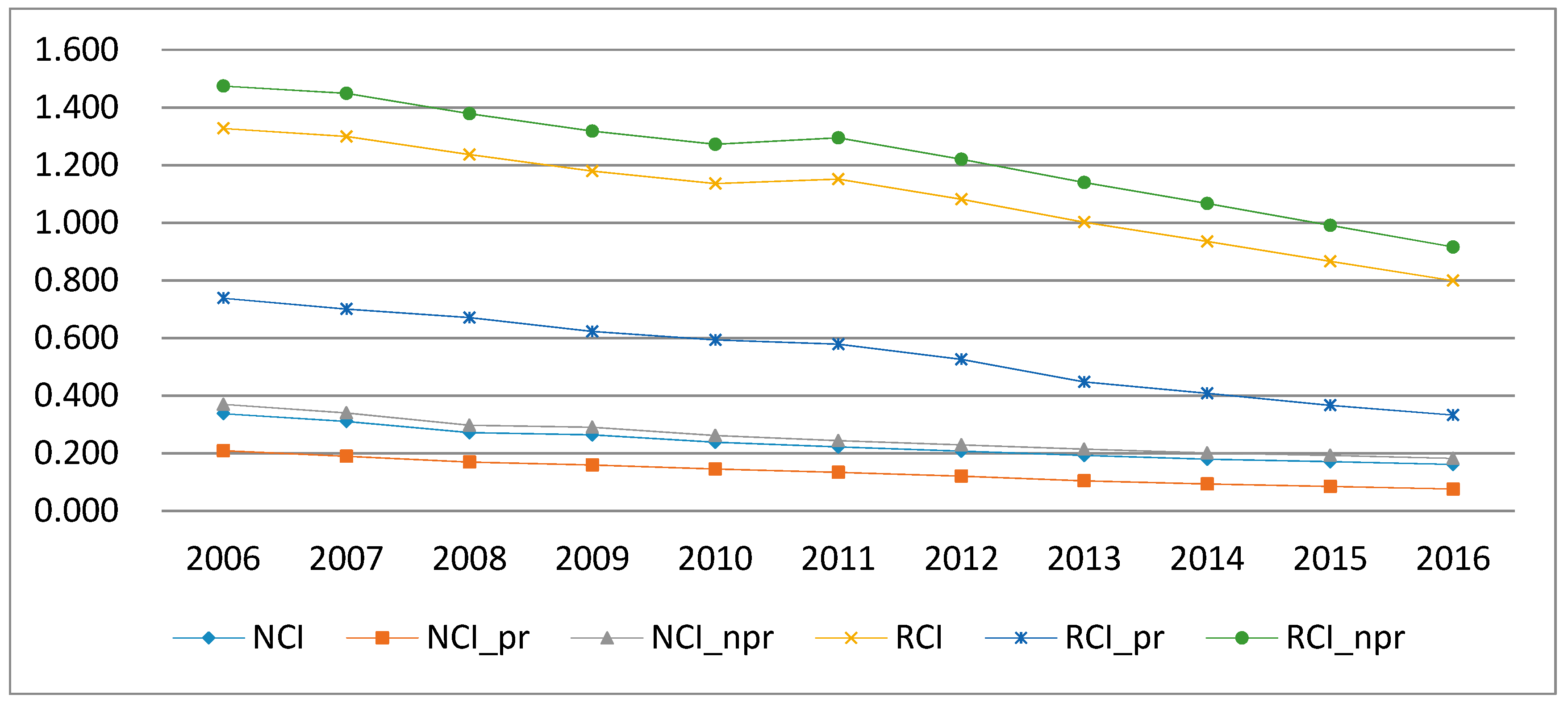
As shown in Figure 2, The CO₂ intensity average of the pilot regions is much lower than that of the non-pilot regions, especially after 2013, no matter calculated by nominal GDP or real GDP. The average nominal CO₂ intensity of the pilot regions decrease by annual 6% from 0.209 to 0.076 t CO₂ per 1000 yuan, during the sample period. In contrast, the non-pilot regions reduce their nominal CO₂ intensity on average by annual 4.6% from 0.37 to 0.183 t CO₂ per 1000 yuan. The average real CO₂ intensity of the pilot regions decrease by annual 5% from 0.739 to 0.333 t CO₂ per 1000 yuan during the sample period. In contrast, the non-pilot regions reduce their real CO₂ intensity on average by 3.5% from 1.475 to 0.903 t CO₂ per 1000 yuan.

After the pilot ETS project, the decreasing rates of the nominal and real CO₂ intensity of the pilot regions are faster than before and also faster than those of the non-pilot regions. The annual decreasing rate of the average nominal CO₂ intensity of the pilot regions is 6% before 2013, and 9.5% after the pilot ETS project. While, the indicator of the non-pilot regions is 5.4% before 2013, and 3.7% during the ETS period. From the aspect of real CO₂ intensity, the annual decreasing rate of the pilot regions is 4.1% before 2013, and 6.4% during the ETS period. The indicator of the non-pilot regions is 2.5% before 2013 and 4.9% during the ETS period. As such, the pilot regions decrease their nominal and real CO₂ intensities faster than the non-pilot regions during the ETS period.

In short, the pilot regions have on average lower CO₂ emissions and intensities than the non-pilot regions and the pilot regions reduced their CO₂ emissions and intensities substantially faster than the non-pilot regions after the pilot ETS project. However, such preliminary observation is insufficient in owing the emissions reduction to the pilot ETS project. An ETS scheme is effective only if it leads to emissions that are lower than would have been the case without the policy. Therefore, an econometric analysis is used to estimate the differential effect of the pilot ETS on CO₂ emissions and intensities versus the case without the pilot ETS project.

4. Empirical Analysis and Discussion

4.1. The Estimation Model

The difference in difference approach (DiD) is a research design for estimating the effects of policy interventions that do not affect everybody at the same time and in the same way, by studying the differential effect of a policy on a treated group versus a non-treated group [22]. Since only a subset of facilities, firms, and regions is selected for the ETS participation, empirical evaluations of the ETS have generally used DiD models to estimate the causal effects of the ETS on treated (i.e., regulated) firms or sectors. The bulk of the relevant literature utilizes the basic DiD model to evaluate the impact of the EU ETS [23]. We use the basic DiD model with control variables and the PSM-DiD model to avoid selection bias in our estimation process.

China announced its pilot ETS project at the end of 2011, but the pilot carbon markets operated in 2013. Therefore, we estimate the causal effects of the pilot ETS project in China by taking 2013 as the tipping point.

Since the pilot regions are very special in terms of their economic development and CO₂ emissions and intensities, the selection does not seem random. To avoid selection bias in the estimation process, three approaches are applied. First, we control for region heterogeneity, by taking economic growth, industrial structure, economic openness, etc. as control variables. Following the DiD specification used by Chan [24], we estimate the causal effects of ETS on emissions abatement based on the following formula:

$$\ln y_{nt}={\beta }_0+{\beta }_{1}ET{S}_{nt}+{\displaystyle \sum \delta X_{nt}+{\phi }_t+{\nu }_n+}{\epsilon }_{nt},n=1,\dots \dots ,30;t=2006,\dots \dots ,2016,$$

(4)

where $y_{nt}$ denotes the CO₂ emissions and intensities for a given province n in year t, as described above. China sets its mitigation target by the CO₂ emissions intensity, which is the emissions per output. Per output can be measured both in nominal GDP and real GDP. Therefore, the dependent variable setting is classified as absolute CO₂ emission, nominal CO₂ emissions intensity and real CO₂ emissions intensity. We specify our model in logarithmic form to interpret the estimates in terms of relative changes. ETS_st is a dummy variable that equals 1 in the years after ETS is launched in province n, and 0 otherwise. Our interest lies in the coefficient ${\beta }_1$ that measures the average treatment effect. We expect a significantly negative estimate of ${\beta }_1$, which suggests that ETS exerts a positive effect on CO₂ abatement. The vector ${\displaystyle \sum X_{nt}}$ is a set of time-varying province-level control variables, described in Section 4.2. ${\phi }_t$ and ${\nu }_n$ are the vectors of year and province dummy variables that account for year and region fixed effects. The year specific dummy variables control for time trends, such as macroeconomic conditions, technical innovation and national changes in energy development strategy, that shape CO₂ emissions over time. Province-specific dummy variables control for time-invariant and unobserved regional characteristics of the pilots relative to the non-pilots. ${\epsilon }_{nt}$ is the idiosyncratic error term.

Then, to avoid self-selection bias, we follow Fowlie [25] in implementing propensity score matching (PSM) to control the difference in ex ante and other important characteristics. PSM would balance the covariates difference between the pilot and non-pilot groups and also provide a similar randomized processing method [26]. The set of control variables, ${\displaystyle \sum X_{nt}}$, is incorporated into the logistic regression model for PSM.

Finally, to demonstrate the robustness of the results, we take the pilot and non-pilot regions as subsamples and compare their differences during the ETS period.

4.2. Control Variables and Data

Regional divergences in economic development and industrial structure have substantial influences on geographical CO₂ emissions. For instance, an inland, less developed region with an economic structure dominated by heavy industry generally consumes more fossil fuels and emits more CO₂ than a high-income coastal region whose economy is services-dominated. To estimate the causal impact of the pilot ETS project on the pilot regions relative to non-pilot regions, confounded variables should be controlled. The control variables are GDP per capita (GDPP_nt), industrial structure (IS_nt, ISS_nt), energy intensity (EI_nt), the level of export (EX_nt) and foreign direct investment (FDI_nt) of a given region n in year t. All control variables are in logarithmic form.

Table 1. Calculation method of control variables.

	Symbol	Variable Explanation	Calculation Method
Control variable	c	nominal GDP Per capita	nominal GDP/population
	RGDPP	real GDP Per capita	real GDP/population
	IS	industrial structure I	added value of the tertiary industry/nominal GDP
	ISS	industrial structure II	added value of the secondary industry/nominal GDP
	EI	energy intensity (inverse of energy efficiency)	energy consumption/real GDP
	EX	export level	gross export/nominal GDP
	FDI	foreign direct investment level	foreign direct investment/nominal GDP

Notes: The gross export volume is measured according to the domestic destination and the source of goods, and its unit is the dollar. Therefore, the unit of gross export is converted into RMB based on the exchange rate of each year.

shows the detailed calculation method of control variables.

The incentive to include GDP per capita is that macroeconomic fluctuations such as the financial crisis affect emissions drastically. Bel [27] demonstrated that the carbon emissions reduction in the EU is due to the economic crisis. Burnett [28] found that personal income drives emission intensities, not absolute emissions in the USA. Previous studies illustrate the experience of developed countries. Whether China follows these rules will be tested in this empirical model. China has published a series of National Working Plans on Controlling Greenhouse Gases since 2006. Sarkodie [29] used nominal GDP per capita (GDP per capita in current US$) to represent economic growth and found an inversed-U shape relationship between CO2 emissions and economic growth in China. Pala et al. [30] took real GDP per capita (GDP per capita constant at 2005 US$) to represent economic activity and found an N-shaped relationship between CO2 emissions and real per capita GDP in China. In this empirical estimations, both nominal GDP per capita and real GDP per capita were used to control economic growth for robustness. We expect negative coefficients for GDP per capita, which stands for the decoupling of emissions from economic development. Industrial structure, energy intensity, exports, and foreign direct investment are taken as control variables following previous theoretical work. The empirical results of Yang [31] indicate that industrial structure is the most significant driving force for CO₂ emissions and energy intensity and has a positive effect on lowering carbon intensity both nationally and regionally in China. The more we use fossil fuels, the larger CO₂ emissions and intensity are. A higher value of energy intensity indicates low energy consumption per GDP, hence a high EI is expected to lower emissions. We therefore expect that the coefficients for energy intensity are positive. Industrial structure I, which is measured by the ratio of the added value of the tertiary industry over nominal GDP, has been increasing in China. It was greater than 50% in 2015. The tertiary industry is less energy-intensive than heavy industry. We therefore expect the coefficients for the industrial structure I to be negative. Industrial structure II is measured by the proportion of the added value of the secondary industry in nominal GDP. The secondary industry is more energy-intensive than the agriculture and tertiary industry. We therefore expect the coefficients for the industrial structure II to be positive. Export and foreign direct investment volume over nominal GDP stand for the level of economic openness. In prior empirical evidence, the effect of FDI on the environment of host developing countries is inconclusive. Hanif [32] found that FDI has triggered carbon emissions and proved the Pollution Haven hypothesis. Abundant evidence shows that FDI induces a decrease in carbon emissions and proves the Pollution Halo effect [33]. In our model, we find the coefficients for foreign direct investment levels to be negative, which means the higher the foreign direct investment level, the more technology and expertise transfer there is, which has a close connection with an economy’s carbon emissions, energy consumption, and foreign trade [34]. Liddle [35] calculated trade openness as imports minus exports and found that trade was significant for consumption-based emissions. Our research studies China’s domestic mitigation policies, which affect territory-based emissions. China is an export-oriented economy and exports have a direct connection with an economy’s territory-based emissions. Therefore, we take the ratio of exports to GDP as a sign of trade openness. The influence of exports on emissions depends on the export structure. Exportation of energy-intensive products increases energy consumption [36]. A high proportion of processing exports decreases energy intensity [37]. The growth of exports has mixed effects on energy consumption and CO₂ emissions.

The data used for the analysis come from the China Statistical Yearbook and the China Energy Statistical Yearbook. The dataset forms an annually balanced panel of 30 provincial administrative regions from 2006 to 2016. All control variables and dependent variables are stationary, which is examined by the Levin, Lin and Chu (LLC), and Phillips–Perron Fisher tests.

4.3. Estimation Results of ETS on Emissions Abatement

Table 2. CO₂ emissions and intensities (results of DiD model).

	lnCE		lnNCI		lnRCI
	(1)	(2)	(3)	(4)	(5)	(6)
Constant	9.180 ***	9.527 ***	0.923 ***	−0.101	2.424 ***	0.655 **
	(7.60)	(9.59)	(10.12)	(−0.23)	(22.97)	(2.24)
ETS	−0.167	−0.14	−0.190 ***	−0.121 **	−0.189 ***	−0.076 *
	(−1.28)	(−1.19)	(−2.90)	(−2.11)	(−3.97)	(−2.03)
lnNGDPP	0.362			−0.208 **
	(1.45)			(−2.28)
lnRGDPP		0.465 (1.58)				0.022 (0.21)
lnIS	−1.883 **	−1.854 **		−0.452		−0.389 **
	(−2.45)	(−2.50)		(−1.24)		(−2.08)
lnEI	−0.035	0.065		0.825 ***		1.045 ***
	(−0.11)	(0.18)		(8.85)		(9.47)
lnEX	0.487 ***	0.437 **		0.222 ***		0.111 *
	(2.90)	(2.41)		(3.60)		(1.75)
lnFDI	−0.291 **	−0.264 **		−0.164 ***		−0.104 **
	(−2.70)	(−2.31)		(−3.34)		(−2.41)
Observations	330	330	330	330	330	330
R2	0.421	0.430	0.271	0.828	0.248	0.924
Controls	Y	Y	N	Y	N	Y

Notes: Controls show control variables are included (Y) or not (N). Values of t-statistics of the coefficients are illustrated in parentheses. ***, ** and * indicate significance at the 1%, 5%, and 10% levels, respectively.

presents the estimated causal effects of the pilot ETS project on CO₂ emissions and intensities. Columns 1 and 2 report the models with lnCE as dependent variable. Column 1 takes the nominal GDP per capita to stand for economic development level, while Column 2 takes the real GDP per capita. In these two regressions, the ETS dummy enters negatively but insignificantly. This suggests ETS has no significant effects on reducing the growth of CO₂ emissions. Columns 3 and 4 report the models with lnNCI as the dependent variable. Column 3 simplifies the conditions without taking control variables. Column 4 includes control variables and uses the nominal GDP per capita to stand for economic development. Columns 5 and 6 report the models with lnRCI as dependent variable. Column 5 excludes control variables. Column 6 takes the real GDP per capita to control the impact of economic developments on real carbon emissions intensity. In these four regressions, the ETS dummy enters negatively and significantly. The results in Column 3 and 5 suggest that ETS induces a 19% decrease in the nominal and real carbon intensities at the 1% significant level. After taking control variables into account, as shown in Column 4 and 6, the estimated treatment effects of ETS are smaller: about 12% decrease in the nominal carbon intensity and 7.6% decrease in the real carbon intensity. Therefore, ETS substantially decreases carbon intensity, no matter measured by nominal or real GDP. The treatment effects of ETS on carbon intensity are still negative and significant even after controlling region heterogeneity.

To investigate the robustness of our findings, we replicated the estimation in Table 2 by substituting the proportion of added value of the secondary industry in GDP (denoted by ISS) for the proportion of added value of the tertiary industry in GDP (denoted by IS) as the symbol of industrial structure upgrading.

Table 3. Effects on CO₂ emissions and intensities (results of DiD model).

	lnCE		lnNCI	lnRCI
	(1)	(2)	(3)	(4)
Constant	12.511 ***	12.608 ***	0.714 **	1.214 **
	(13.91)	(15.59)	(2.17)	(4.97)
ETS	−0.132	−0.127	−0.112 **	−0.074 **
	(−1.02)		(−2.07)	(−2.13)
lnNGDPP	0.125 (0.57)		−0.266 *** (−2.77)
lnRGDPP		(-0.97)		−0.029
		0.155		(−0.29)
lnISS	1.759 **	1.733 **	0.439 *	0.264 *
	(2.67)	(2.58)	(1.70)	(1.80)
lnEI	−0.201	−0.167	0.783 ***	1.011 ***
	(−0.74)	(−0.52)	(7.89)	(8.88)
lnEX	0.390 **	0.376 **	0.199 ***	0.098
	(2.41)	(2.11)	(3.20)	(1.50)
lnFDI	−0.288 **	−0.280 **	−0.164 ***	−0.105 **
	(−2.53)	(−2.28)	(−3.44)	(−2.40)
Observations	330	330	330	330
R2	0.487	0.487	0.836	0.922
Controls	Y	Y	Y	Y

Notes: The variables in this table are the same as in Table 2 except ISS is substituted for IS. Controls show control variables are included (Y) or not (N). Values of t-statistics of the coefficients are illustrated in parentheses. ***, ** and * indicate significance at the 1%, 5%, and 10% levels, respectively.

shows the results. The estimated treatment effects of ETS and the corresponding t-values are similar to those reported in Table 2. We also find that the pilot ETS project has significantly induced the decrease of nominal and real CO₂ intensities, but its negative effects on CO₂ emissions are not significant.

The estimated results for control variables remain unchanged, as shown in Table 2; Table 3. This suggests that the influence of the control variables on CO₂ emissions and intensities are robust. As expected, the proportion of tertiary industry in GDP (lnIS) has significantly negative effects, while the effects of the proportion of secondary industry in GDP (lnISS) are significantly positive. Export level (lnEX) has significantly positive influences. The level of foreign direct investment (lnFDI) has significantly negative effects. As for nominal economic growth per capita (lnNGDPP), the results suggest that it reduces the growth of nominal CO₂ intensity significantly, but has an insignificantly positive effect on the growth of CO₂ emissions. The real economic growth per capita (lnRGDPP) has negative effects on CO₂ emissions and real CO₂ intensity; however, these are statistically insignificant. Energy intensity (lnEI) has positive impacts on nominal and real CO₂ intensities, at the 1% significance level. However, if we examine its effects on CO₂ emissions this picture changes. We do not find a statistically significant relationship between energy intensity and CO₂ emissions. Energy intensity is the reciprocal value of energy efficiency. Thus, the results suggest that the improvement of energy efficiency has significantly decreased the nominal and real CO₂ intensities. However, it has an insignificant effect on CO₂ emissions.

We also perform a robustness test by using semi-parametric DiD model. We apply matching methods with bootstrap procedures to identify a comparable non-treated group of provinces. Then we use the DiD model in order to estimate the effects of the pilot ETS project with control variables. The estimation results of PSM-DiD is shown in

Table 4. CO₂ emissions and intensities (results of PSM-DiD model).

	lnCE		lnNCI	lnRCI
	(1)	(2)	(3)	(4)
Region	−0.294 **	−0.327 **	−0.081	−0.167 ***
	(−2.20)	(−2.08)	(−1.26)	(−2.87)
ETS	−0.057	−0.203	−0.259 **	−0.195 *
	(−0.24)	(−0.95)	(−2.38)	(−1.68)
Controls	Y	Y	Y	Y

Notes: t statistics are shown in the respective parentheses. * p < 0.1, ** p < 0.05, *** p < 0.01. In Column 1, the covariates incorporated in the logistic regression model for PSM are lnNGDPP, lnIS, lnEI, lnEX, lnFDI. In Column 2, we substitute lnRGDPP for lnNGDP. In the regression of lnNCI, the covariates incorporated in the logistic regression model for PSM are lnNGDPP, lnIS, lnEI, lnEX, lnFDI. In the regression of lnRCI, lnNGDPP are replaced by lnNGDP.

. The coefficients for ETS are also significantly negative in the regressions of lnNCI and lnRCI, while in the regressions of lnCE are insignificant. We find consistent results for all estimations.

To ensure the estimators of the average treatment effect are unbiased, we do subsample research. In the analysis of the pilot subsample and non-pilot subsample, the results in

Table 5. CO₂ emissions and intensities of subsamples (results of DiD model).

	lnCE					nNCI		lnRCI
	Pilot (1)	Non-Pilot (2)	Pilot (3)	Non-Pilot (4)	Pilot (5)		Non-Pilot (6)	Pilot (7)	Non-Pilot (8)
Time	−0.285	−0.005	−0.203	−0.052	−0.971 *		−0.003	−0.277 *	−0.071
	(−0.51)	(−0.04)	(−1.38)	(−0.45)	(−1.69)		(−0.02)	(−1.97)	(−0.65)
lnNGDPP	0.861 ***	0.768 ***			−0.145 *		−0.272 ***
	(10.06)	(22.40)			(−1.66)		(−8.09)
lnRGDPP			1.183 ***	1.139 ***				0.194 **	0.089 *
			(12.66)	(23.61)				(2.17)	(1.93)
Observations	66	264	66	264	66		264	66	264
R2	0.903	0.875	0.934	0.882	0.982		0.928	0.983	0.882
Controls	Y	Y	Y	Y	Y		Y	Y	Y
Controls$\times$time	Y	Y	Y	Y	Y		Y	Y	Y

Notes: t-statistics are shown in the respective parentheses. * p < 0.1, ** p < 0.05, *** p < 0.01. The columns with odd numbers show the regression results of pilot subsample. The columns with even numbers show the regression results of non-pilot subsample.

show that the trends of time are all negative across the pilot regions and non-pilot regions. This suggests that the time trend of CO₂ emissions and intensities are the same for the pilots and non-pilots after the pilot ETS program started. In the pilot subsample, the time dummy has significantly negative effects on the nominal and real CO₂ intensity, but they are insignificant in the non-pilot subsample. The results are in line with the analysis in Section 3. Hence, all these examinations show that the pilot ETS project has positive effects on CO₂ abatement. ETS is significant to nominal and real CO₂ intensities, but insignificant to CO₂ emissions. The result is robust.

4.4. Estimation Results of ETS on Energy Consumption Structure

We apply the DiD models to estimate the causal effects of the pilot ETS project on improving energy consumption structure, to figure out the mechanism of the ETS reducing emissions. Energy consumption structure has a direct influence on CO₂ abatement. Among fossil fuels, natural gas has the lowest carbon emissions coefficient and coal has the highest. China is rich in coal but poor in oil and natural gas. Thus, the main way the pilot ETS project attempts to induce emissions abatement is by replacing coal with other relatively low-carbon fossil fuels. We take the proportions of coal, petroleum, and natural gas to total energy consumption as dependent variables. COA is the share of coal consumption. PET is the share of petroleum consumption. NAG is the share of natural gas consumption.

Table 6. Energy consumption structure (results of DiD model).

	lnCOA	lnPET	lnNAG
Constant	−0.756 *	−2.852 ***	−6.150 ***
	(−1.71)	(−6.52)	(−5.82)
ETS	−0.284 **	0.045	0.093
	(−2.32)	(0.53)	(0.68)
lnRGDPP	−0.120	0.201	0.931 ***
	(−0.89)	(1.54)	(3.03)
lnIS	−0.953 **	0.834 *	1.101
	(−2.32)	(2.02)	(1.02)
lnEX	0.102	0.057	−0.594 ***
	(0.91)	(0.49)	(−3.15)
lnFDI	−0.154 *	0.075	0.357 **
	(‒1.92)	(0.83)	(2.72)
Observations	330	330	330
R2	0.429	0.349	0.266
Controls	Y	Y	Y

presents the estimated causal effects of the pilot ETS project on energy consumption structure, using DiD models. The results in Column 1 suggest that ETS induces a 28% decrease in the proportion of coal to total energy consumption at the 5% significance level. The estimated treatment effects of ETS on the proportion of petroleum and natural gas to total energy consumption are negative but insignificant.

The estimation results of PSM-DiD, shown in

Table 7. Energy consumption structure (results of PSM-DiD model).

	lnCOA	lnPET	lnNAG
Pilot	−0.169***	0.184	0.409*
	(−3.99)	(1.46)	(1.65)
ETS	−0.174**	−0.085	−0.295
	(−2.22)	(−0.53)	(−0.75)
Controls	Y	Y	Y

, suggest that the results are robust. The pilot ETS project has significantly improved the energy consumption structure. Decreasing the proportion of coal to total energy consumption may be the main way the pilot ETS projects induces emission abatement.

5. Conclusions and Future Research

We employ the DiD approach to investigate the abatement effects of the pilot ETS project in China. Using the fossil fuel data of 30 provincial administration regions from 2006 to 2016, we estimate the fossil CO₂ emissions and intensities of each province. The results show that the average CO₂ emissions and intensities in the pilot regions are lower than those in the non-pilot regions and the pilot regions substantially abate their CO₂ emissions and intensities on a larger scale than the non-pilot regions under the pilot ETS project.

Nevertheless, the abatement effects of the pilot ETS project on the fossil CO₂ emissions and CO₂ intensities are asymmetrical; the reduction effects on the latter are significant, whereas for the former they are not. We find strong empirical evidence suggesting that the pilot ETS project has a significant causal impact on reducing nominal and real CO₂ intensity. The pilot ETS project induces around a 12% decrease in nominal CO₂ intensity and a 7% decrease in real CO₂ intensity, but its negative effect on CO₂ emissions is insignificant. The pilot ETS project has significant effects on decreasing the proportion of coal to total energy consumption, which may be the main way the pilot ETS project induces CO₂ abatement. We will further explore the mechanism of ETS influencing abatement at a firm level, especially the mechanism of ETS limiting the total quantity of CO₂ emissions. The diversified policy design of the pilot ETS in China and its impact on the effectiveness of ETS will also be addressed in future research.

In addition, the estimated results for control variables show that the proportion of tertiary industry in GDP (lnIS) and the level of foreign direct investment (lnFDI) have significantly negative effects on CO₂ emissions and intensities, while the effects of the proportion of secondary industry in GDP (lnISS) and the export level (lnEX) are significantly positive. Therefore, upgrading the industrial structure, attracting FDI, and purifying the export structure in terms of environmental degradation have significant effects on abatement. The design of the national ETS should be in line with industrial and opening-up policies. The interaction of these policies on emission abatement should be addressed in future research.

References

- Ellerman, D.; Buchner, B. The European Union Emissions Trading Scheme: Origins, Allocation, and Early Results. Rev. Environ. Econ. Policy 2007, 1, 66–87. [Google Scholar] [CrossRef]
- Ellerman, D.; Buchner, B. Over-allocation or abatement? A preliminary analysis of the EU ETS based on the 2005–06 emissions data. Environ. Resour. Econ. 2008, 41, 267–287. [Google Scholar] [CrossRef]
- Lo, A.Y. Challenges to the development of carbon markets in China. Clim. Policy 2016, 16, 109–124. [Google Scholar] [CrossRef]
- Wang, X.; Xue, M.; Xing, L. Analysis of Carbon Emission Reduction in a Dual-Channel Supply Chain with Cap-And-Trade Regulation and Low-Carbon Preference. Sustainability 2018, 10, 580. [Google Scholar] [CrossRef]
- Zhao, X.; Zhang, Y.; Liang, J.; Li, Y.; Jia, R.; Wang, L. The Sustainable Development of the Economic-Energy-Environment (3E) System under the Carbon Trading (CT) Mechanism: A Chinese Case. Sustainability 2018, 10, 98. [Google Scholar] [CrossRef]
- Petrick, S.; Wagner, U.J. The Impact of Carbon Trading on Industry: Evidence from German Manufacturing Firms. Kiel Work Paper. 2014. Available online: https://ssrn.com/abstract=2389800 (accessed on 4 February 2019).
- Martin, R.; Muûls, M.; Wagner, U.J. The Impact of the European Union Emissions Trading Scheme on regulated firms: What is the evidence after ten years? Rev. Environ. Econ. Policy 2016, 10, 129–148. [Google Scholar] [CrossRef]
- Jaraite, J.; Di Maria, C. Did the EU ETS Make a Difference? An Empirical Assessment Using Lithuanian Firm-Level Data. CERE Working Papers 2. 2014. Available online: http://dx.10.5547/01956574.37.2.jjar (accessed on 4 February 2019).
- Mezosi, A.; Pato, Z.; Szabo, L. Assessment of the EU 10% interconnection target in the context of CO2 mitigation. Clim. Policy 2016, 16, 658–672. [Google Scholar] [CrossRef]
- Laing, T.; Sato, M.; Grubb, M.; Comberti, C. The effects and side-effects of the EU emissions trading scheme. Wiley Interdiscip. Rev. Clim. Chang. 2014, 5, 509–519. [Google Scholar]
- Lofgren, A.; Wrake, M.; Hagberg, T. Why the EU ETS needs reforming: An empirical analysis of the impact on company investments. Clim. Policy 2014, 14, 537–558. [Google Scholar] [CrossRef]
- Teng, F.; Wang, X.; Lv, Z. Introducing the emissions trading system to China’s electricity sector: Challenges and opportunities. Energy Policy 2014, 75, 39–45. [Google Scholar] [CrossRef]
- Zhao, X.; Jiang, G.; Nie, D.; Chen, H. How to improve the market efficiency of carbon trading: A perspective of China.Renew. and Sustain. Energy Rev. 2016, 59, 1229–1245. [Google Scholar]
- Lo, A.Y. Carbon trading in a socialist market economy: Can China make a difference? Ecol. Econ. 2013, 87, 72–74. [Google Scholar] [CrossRef]
- Zhou, P.; Zhang, L.; Zhou, D.Q.; Xia, W.J. Modeling economic performance of interprovincial CO2 emission reduction quota trading in China. Appl. Energy 2013, 112, 1518–1528. [Google Scholar] [CrossRef]
- Cui, L.B.; Fan, Y.; Zhu, L.; Bi, Q.H. How will the emissions trading scheme save cost for achieving China’s 2020 carbon intensity reduction target? Appl. Energy 2014, 136, 1043–1052. [Google Scholar] [CrossRef]
- Wang, P.; Dai, H.; Ren, S.; Zhao, D.; Masui, T. Achieving Copenhagen target through carbon emission trading: Economic impacts assessment in Guangdong Province of China. Energy 2015, 79, 212–227. [Google Scholar] [CrossRef]
- Wang, K.; Wie, Y.M.; Huang, Z. Potential gains from CO2 emissions trading in China: A DEA based estimation on abatement cost savings. Omega 2016, 63, 48–59. [Google Scholar] [CrossRef]
- Huang, Y.; Liu, L.; Ma, X.; Pan, X. Abatement technology investment and emissions trading system: A case of coal-fired power industry of Shenzhen, China. Clean Technol. Environ. Policy 2015, 17, 811–817. [Google Scholar] [CrossRef]
- Liu, Y.; Tan, X.; Yu, Y.; Qi, S. Assessment of impacts of Hubei Pilot emission trading schemes in China—A CGE-analysis using Term CO2 model. Appl. Energy 2017, 189, 762–769. [Google Scholar] [CrossRef]
- IPCC. Greenhouse Gas Inventory: IPCC Guidelines for National Greenhouse Gas Inventories; United Kingdom Meteorological Office: Bracknell, England, 2006.
- Imbens, G.W.; Wooldridge, J.M. Recent developments in the econometrics of program evaluation. J. Econ. Lit. 2009, 47, 5–86. [Google Scholar] [CrossRef]
- Clo, S. The effectiveness of the EU Emissions Trading Scheme. Clim. Policy 2009, 9, 227–241. [Google Scholar] [CrossRef]
- Chan, H.S.; Li, S.; Zhang, F. Firm Competitiveness and the European Union Emissions Trading Scheme. Energy Policy 2013, 63, 1056–1064. [Google Scholar] [CrossRef]
- Fowlie, M.; Stephen, P.H.; Erin, M. What do emissions markets deliver and to whom? evidence from southern california’s NOx trading program. Am. Econ. Rev. 2012, 102, 965–993. [Google Scholar] [CrossRef]
- Rosenbaum, P.; Rubin, D. The central role of the propensity score in observational studies for casual effects. Biometrika 1983, 701, 41–55. [Google Scholar] [CrossRef]
- Bel, G.; Joseph, S. Emission abatement: Untangling the impacts of the EU ETS and the economic crisis. Energy Econ. 2015, 49, 531–539. [Google Scholar] [CrossRef]
- Burnett, J.W.; Bergstrom, J.C.; Wetzstein, M.E. Carbon dioxide emissions and economic growth in the US. J. Policy Model. 2013, 35, 1014–1028. [Google Scholar] [CrossRef]
- Sarkodie, S.A.; Vladimir, S. Empirical study of the Environmental Kuznets curve and Environmental Sustainability curve hypothesis for Australia, China, Ghana and USA. J. Clean. Prod. 2018, 201, 98–110. [Google Scholar] [CrossRef]
- Pala, D.; Subrata, K.M. The environmental Kuznets curve for carbon dioxide in India and China: Growth and pollution at cross road. J. Policy Model. 2017, 39, 371–385. [Google Scholar] [CrossRef]
- Yang, Y.; Yannan, Z.; Jessie, P.; Ze, H. China’s carbon dioxide emission and driving factors: A spatial analysis. Clim. Policy J. Clean. Prod. 2019, 211, 640–651. [Google Scholar] [CrossRef]
- Hanif, I.; Syed, M.F.R.; Pilar, G.S.; Qaiser, A. Fossil fuels, foreign direct investment, and economic growth have triggered CO2 emissions in emerging Asian economies: Some empirical evidence. Energy 2019, 171, 493–501. [Google Scholar] [CrossRef]
- Zarsky, L. Havens, halos and spaghetti: Untangling the evidence about foreign direct investment and the environment. For. Dir. Invest. Environ. 1999, 13, 47–74. [Google Scholar]
- Shahzad, S.J.H.; Kumar, R.R.; Zakaria, M. Carbon emission, energy consumption, trade openness and financial development in Pakistan: A revisit. Renew. Sustain. Energy Rev. 2017, 70, 185–192. [Google Scholar] [CrossRef]
- Liddle, B. Consumption-Based Accounting and the Trade-Carbon Emissions Nexus in Asia: A Heterogeneous, Common Factor Panel Analysis. Sustainability 2018, 10, 3627. [Google Scholar] [CrossRef]
- Yu, H. The influential factors of China’s regional energy intensity and its spatial linkages: 1988–2007. Energy Policy 2012, 45, 583–593. [Google Scholar] [CrossRef]
- Jiang, X.; Duan, Y.; Green, C. Regional disparity in energy intensity of China and the role of industrial and export structure. Res. Conserv. Recycl. 2017, 120, 209–218. [Google Scholar] [CrossRef]
Figure 1.
CO2 emissions in China from 2006 to 2016 (unit: million tons). Note: CE is the national average of CO2 emissions. CE-pr is the average CO2 emissions of the pilot regions. CE-npr is the average CO2 emissions of the non-pilot regions.
Figure 2.
Nominal and real CO2 intensities in China during 2006‒2016 (unit: tons/1000 yuan). Note: NCI is the national average of nominal CO2 intensity. NCI-pr is the average nominal CO2 intensity of the pilot regions. NCI-npr denotes the average nominal CO2 intensity of the non-pilot regions. RCI is the national average of real CO2 intensity. RCI-pr is the average real CO2 intensity of the pilot regions. RCI-npr denotes the average real CO2 intensity of the non-pilot regions.