Performance Analysis of a Polling-Based Access Control Combining with the Sleeping Schema in V2I VANETs for Smart Cities

Abstract

In vehicular ad hoc networks (VANETs), one of the important challenges is the lack of precise mathematical modeling taking into account the passive vacation triggered by the zero-arrival state of nodes. Therefore, a polling-based access control is proposed in this paper using a sleeping schema to meet the challenge of quality of service (QoS) and energy-efficient transport in VANET environments for smart cities. Based on IEEE 802.11p, it was developed in an attempt to improve the energy efficiency of the hybrid coordination function of controlled channel access (HCCA) through a self-managing sleeping mechanism for both the roadside unit (RSU) and on-board units (OBUs) or sensor nodes according to the traffic load in vehicle -to-infrastructure (V2I) scenarios. Additionally, a Markov chain was developed for analyzing the proposed mechanism, and the exact mathematical model is provided with regard to the passive vacation. Then, the performance characteristics—including the mean cyclic period, delay, and queue length—were accurately obtained. In addition, the closed-form expression of the quantitative relationship among sleeping time, performance characteristics, and service parameters was obtained, which can easily evaluate the energy efficiency. It was proven that theoretical calculations were completely consistent with simulation results. The simulation results demonstrate that the suggested method had much lower energy consumption than the standard strategy at the expense of rarely access delay.

1. Introduction

As a key symbol of smart cities, intelligent and connected transportation systems (ICTSs) are growing rapidly, and so vehicular ad hoc networks (VANETs) have attracted a great deal of attention in the research community because of their contributions to road safety, traveling support, traffic efficiency, user-oriented service, etc. [1,2]. Urgent information, traffic-related information, and entertainment information are exchanged either between on-board units (OBUs) in vehicle-to-vehicle (V2V) scenarios or between OBUs (or sensor nodes) and infrastructure in vehicle-to-infrastructure (V2I) environments. Furthermore, data collected on the road can be forwarded to any other data centers through vehicle-to-everything (V2X) communications [3].

Connectivity and security are major concerns in V2V communications, as all the communication parameters rely on neighboring participants, such as wireless technologies and relative speed that play an important role in communication performance [4]. In V2I, roadside units (RSUs) are usually located apart from each other along the sideways to provide safety service and traffic management in urban or highway environments. Unlike the high-throughput and broad bandwidth requirements in user-oriented applications, safety services and traffic management messages are exchanged between vehicles and the roadside, which emphasizes the need for low access delay and transmission delays to provide the highest possible level of safety. Gristiano M. Silva et al. investigated the limitations and challenges associated with such infrastructure-based vehicular communications [5]. In the IEEE 802.11p standard, the hybrid coordination function of controlled channel access (HCCA) uses a collision-free polling scheme to provide the bounded delays for real-time applications. However, this may lead to resource overshooting, especially for low-load scenarios.

The passive vacation arising from the zero-arrival state often occurs when system load is not heavy, in which nodes can be allowed to sleep. Moreover, the sleeping schema is very useful in achieving a green environment because it helps to reduce unnecessary energy consumption and channel resources occupation, even if the nodes can be easily charged. In [6], a periodical sleeping and awakening mechanism on stations (STAs) was used in the Power Save (PS) model in order to save energy at the cost of data transmission during the sleep state. Transmission Opportunity Power Save Mode (TXOP PSM) can greatly improve the energy efficiency of STAs in highly dense networks and with heavy traffic conditions. In fact, traffic oscillation properties are significant in both temporal and spatial domains. Therefore, frequent transmission and idle listening from the RSUs cause much power to be lost. Unfortunately, most of the proposals in the power-saving do not take the RSUs into account.

On the other hand, although many sleeping-based power-saving mechanisms were studied, most of them were based only on computer simulations or energy consumption models [7,8], or only the maximum achievable energy efficiency was analyzed. However, the passive vacation or sleeping state resulting from the zero-arrival state of nodes is rarely considered during system modeling, which has led to a decrease in accuracy [9]. This situation requires a theoretical model that can easily assess the quantitative relationship among system performance, sleeping factor, and network control parameters.

Accordingly, considering the passive vacation, a k-limited ($k=1$) polling-based access control protocol with the sleeping technique named Polling Control with Sleeping (PC-S) media access control (MAC) is proposed in this paper for V2I VANETs. A self-managing sleeping mechanism is used for both RSUs and OBUs (or nodes) to improve the energy efficiency of HCCA according to the traffic load. For those OBUs or sensor nodes with transmission requirements, RSU notifies and updates the reserved service slots, respectively depending on their registered sequence. As a result, the nodes can turn off the radio transceivers to save energy and just wake up on their service slots. When none of the nodes request to transmit data and wake up after a sleeping period, the RSUs also turn to sleep or can maintain a low-power waiting state to deal with critical messages.

In addition, the relationship between system performance characteristics and sleeping period will be examined in this study. The mathematical model of PC-S will be adjusted using the embedded Markov chain theory and the probability generating function. It should be noted that for the first time, the precise expressions of the first-order and high-order performance characteristics with the sleeping factor (e.g., the mean cyclic period, the queue length at polling epoch, the mean waiting time, and the queue length) are obtained in this study. As will be shown, the calculation deviation was reduced from more than 9% to almost zero compared to the standard strategy.

The rest of the paper is organized as follows: Section 2 provides an overview of VANETs in ICTS and related work. The proposed model is presented in Section 3. Section 4 contains a detailed analysis of the generating functions and the relationship between sleeping period and network performance. Numerical examples are also presented in Section 5 that provide insight into performance behavior and energy consumption. Finally, Section 6 concludes the paper.

2. Related Work

In VANET communication, several media access control (MAC) protocols are designed that can be cataloged as contention-based, contention-free-based, and hybrids of the previous two. In recent years, some advances have been made in the field of MAC for VANETs based on IEEE 802.11p (802.11p for short) [10]. Enhanced distributed coordination access (EDCA) at 802.11p is sufficiently flexible to deal with high mobility and frequent topological changes. However, it is completely decentralized, and random access features include deficiencies in strict timing and reliability, which makes it unfeasible in safety-critical applications. To overcome these problems, several MAC protocols based on time division multiple address (TDMA) are presented [10,11]. An overview of TDMA-based MAC protocols for VANETs is given in [2]. In 802.11p, the hybrid coordination function (HCF) of controlled channel access (HCCA) mechanism employs a polling scheme because of its ability to guarantee high QoS, which is essential for emergency information and some traffic related information delivery in vehicular environments. In current 802.11p HCCA, as with the point coordination function (PCF) in IEEE 802.11 for wireless local area networks (WLANs), if an OBU does not have any packet for transmitting, it will either send a null frame, or will send nothing back to the RSU. Idle polling will lead to resource dissipation and overshooting, and further it is a waste of energy. To enhance the channel utilization, a dynamic polling method has been proposed in [12], in which the central HCF coordinator assigned the TXOP dynamically by gathering requirements from the OBUs, even there was an improvement in throughput and delay. However, the complexity of HC scheduling was increased from O(n) to O(n2). In [13], a token passing approach on top of a random access MAC protocol is proposed to prevent channel contention and improve the reliability of the safety message transmissions. Although these protocols have improved the delay performance or beacon delivery ratio in VANETs, most of the analyses were done by simulation. Therefore, the lack of accurate and scalable models to achieve the quantitative relationship between quality of service (QoS) and network parameters is still felt.

According to the performance analysis, the superframe is employed in [14] to cut down the number of polling frames and improve the performance of a highly loaded system, but the idle energy consumption is ignored. In [15], the M/G/1 vacation model is introduced to analyze the latency feature of IEEE 802.11 PCF. However, the authors only considered the regular periodical vacation of the server. It did not matter if the nodes were idle or not, which could increase the delay when the nodes were not idle. In [16], the queue length distribution in the K-limited polling service is discussed using an iterative approximation, regardless of the sleep state. In [7], the GreenPoll MAC protocol combining the TXOP PSM with reservation and implicit polling is proposed to save power, but the node must take some energy to detect its transmission slots by overhearing the channel before it exchanges data with the access point (AP). Moreover, only the computation model for energy consumption analysis is presented, ignoring the system model.

To reduce energy consumption, some researchers have proposed some sleep strategies in the literature to minimize the effect of the sleeping mechanisms on system performances [17,18,19,20,21,22,23,24,25,26,27,28]. In [17,18], a sleeping/awakening mechanism with loose synchronization was proposed to extend the lifetime of the nodes by reserving long-length-frame sending, but the delay also increased. In [19], a method of slots reservation is used to save energy and improve system throughput in a burst traffic scenario by dividing the service time into periodic requests and sending-out slots. In order to reduce the delay, both the energy consumption and the packets are considered in [23] for updating the vacation period dynamically. In [25], a dispatching control scheduler to build an architectural health monitoring sensor network was suggested to save energy and reduce the end-to-end delay by deploying the father link based on the children links’ occupying on the routing tree. In [26], the scheduling lists of neighbors are collected to reduce consumption. In another study [27], a self-adapted sleep scheme is proposed to follow the changing traffic dynamics. In [28], the periodic polling system of the limited service is analyzed theoretically, but the zero-arrival state and the following sleep state is neglected in the mathematical model. In [29], the sleep state is combined into the mathematic model for the first time, and the expression of the mean cyclic period, first-order performance characteristic is obtained. However, the mathematical expressions of the high-order performance characteristics have not yet been obtained, let alone the relationship between performance and sleep period.

Therefore, to the best of our knowledge, none of the previous works have analyzed the performance characteristics theoretically using the sleep state in a mathematical model that simultaneously considers the energy efficiency. Therefore, in this paper, the PC-S, which is a 1-limited polling-based access control protocol with sleeping technique, is proposed for V2I VANETs. A sleeping technique (as will be described in Section 3.3) is applied to both OBUs and RSU. In addition, the mathematical model of PC-S is set so that the quantitative relationship between system performance and network control parameters can be easily evaluated.

3. Mechanism of PC-S

In this section, the access control mechanism of PC-S is described, including application vehicular environment, service mechanism, and sleeping technique.

3.1. Network Environment

Here, a mobile vehicular environment will be considered where the OBUs or nodes in the cluster have three different types:

• Applicant Node (AN): An OBU or a sensor node that has applied to join the cluster;
• Cluster Member (CM): An OBU or a sensor node that has been joined to the cluster and has been added to the polling list table;
• Dissociative Node (DN): An OBU or a sensor node that has left the current cluster, but has not yet joined the other.

In Figure 1, an example of the proposed polling-based structure is presented. OBUs and other environmental sensor nodes in the coverage of the RSU form a cluster by a distance-based clustering algorithm, in which the RSU acts as a cluster header. Under the mechanism of PC-S, OBUs and sensor nodes can enter a sleep state and wake up at the time slot allocated by the RSU for sending its uplink messages. Furthermore, in some of spare cases, if none of the nodes in the cluster have data to transmit, the RSU will also go to sleep until the next round of transmission. Active RSUs in neighborhood work under different SCHs to prevent frequency interference.

3.2. 1-Limited Polling Access Mechanism

An HCCA superframe consists of a contention-free period (CFP) and a contention period (CP). For safety services and traffic management with a highly real-time requirement, data packets are delivered by a polling scheme in CFP with a high-level QoS guarantee. The user-oriented service data packets transmission and cluster update are executed at the CP phase.

During the CFP, the RSU broadcasts a beacon with cluster ID, user ID, and NAV time at the beginning of the CFP. It can also deliver downlink data packets after the beacon.

An immigrating OBU or a node with a transmission requirement (i.e., AN) will send an application to join the cluster after receiving the CFP_END (CE) frame. The RSU will assign a user ID for each AN, and broadcast in the beacon. Then, ANs turn into CMs after receiving their user ID and will be polled in a round robin fashion during the CFP, as shown in Figure 2. CMs will hold their user ID until leaving the current cluster. If a CM moves outside the coverage of the cluster head and still has transmission requirement, it will apply to join another cluster and be treated as an AN. Otherwise, it will be a DN.

All CMs receive the beacon to update the network allocation vectors (NAVs). On the PC-S MAC network, OBUs and nodes can deliver either one uplink data or null data with constant packet length when receiving a polling frame from the RSU. CMs inform the RSU of their buffer states in the ACK frame during visit periods. In the successive CFP, the RSU will not poll the CM that has declared its idle state.

3.3. Sleeping Technique

In the 802.11p standard, an OBU must respond within a short interframe space (SIFS) period once it receives a polling frame from the Hybrid Coordinator (HC) in the CFP duration. When the OBU or sensor node does not have any queued packet to send, it will send back a null frame, which is a waste of channel resources and energy consumption. Obviously, continuous interception and polling from the RSU in a completely empty network would be a serious energy waste. On the other hand, idle listening and null frame transmission from OBUs or sensor nodes would take up a large amount of channel resources.

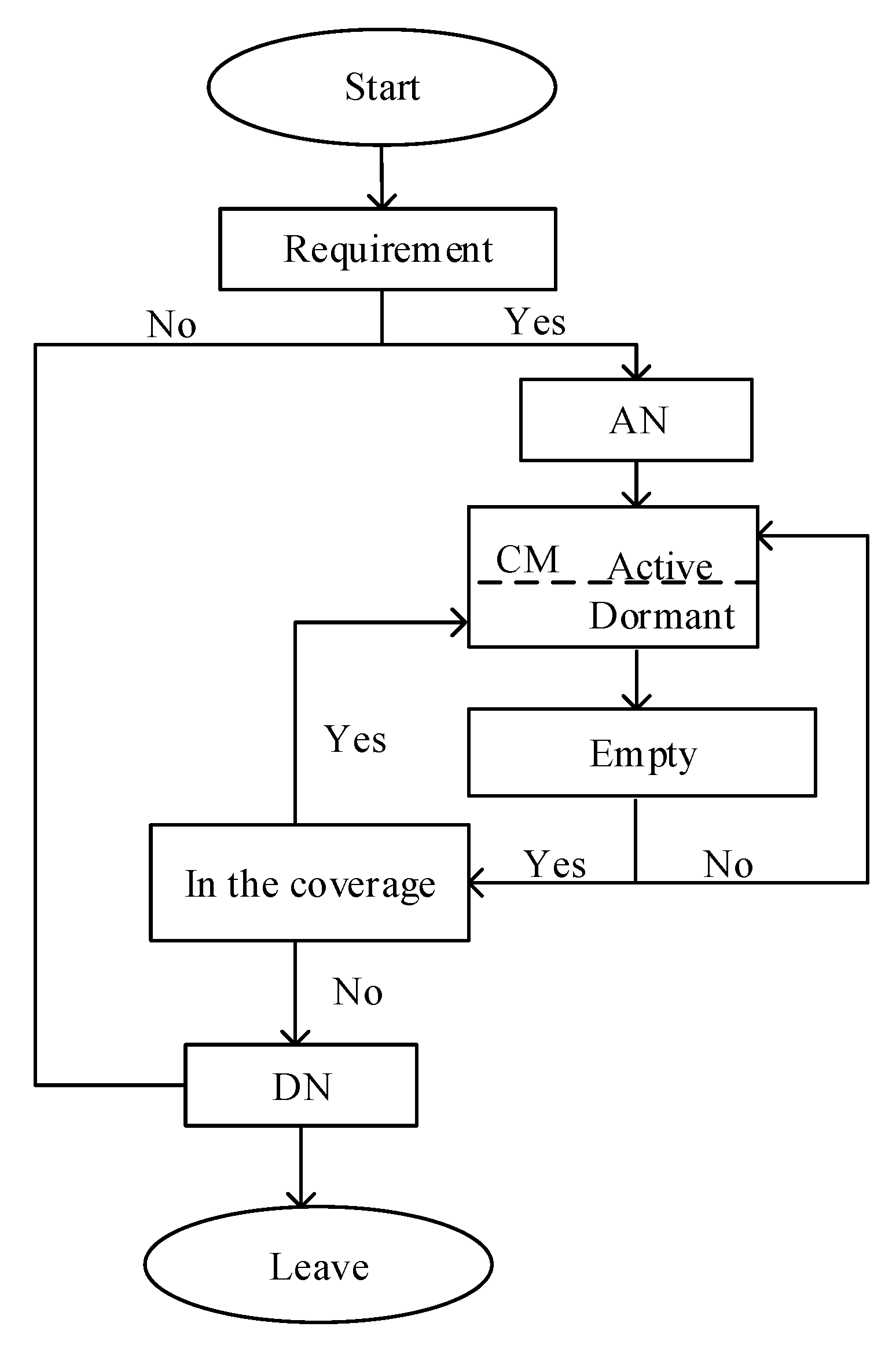
In PC-S, the sleeping technique is used for both OBUs and the RSU. An OBU or a node will soon be in sleep state upon completion of the transmission and will announce its state to the RSU in the ACK. The RSU will not poll the sleeping OBU until new arrivals awaken it. As shown in Figure 3, the state transition is as follows:

• For an RSU, it broadcasts a beacon frequently as long as there is at least one active OBU/node in the coverage area.
• A vehicle/sensor node in the coverage starts as an AN, and then it becomes a CM when it has communication requirement and is added to the polling list by an RSU.
• A CM waits for the polling from an RSU, and becomes a DN it is once beyond the communication coverage or finishes all the data transmission.
• A CM will turn into sleep state as it has finished the entire data transmission, and will wake up when it has new requirements.

When the RSU’s polling list is empty (i.e., no active OBUs or nodes in the cluster), the RSU can choose to set a timer and go to sleep after sending a beacon frame, or it can remain in an active state to respond immediately.

4. Mathematical Model of PC-S and Performance Evaluation

In this section, the mathematical model of PC-S is obtained and the explicit expressions of the system performance characteristics are derived.

4.1. Outline

Most of the existing works in the literature have analyzed the performance of the HCCA-based medium access mechanism using simulations. To model the relationship among system parameters such as the sleeping period, traffic load, and the QoS, we expand the classical discrete-time 1-limited polling model to analyze the performance of PC-S. The service model can be described as follows:

In a cycle of service, an AP (i.e., an RSU) serves the node (i.e., sensor nodes and OBUs) in its polling list table one by one with a 1-limited service strategy in a subnet. The AP authorizes the channel to the polled node in turn. If the current node does not have any requests for data transmission or no response, the AP will poll the next node because it thinks the current node is sleeping or outside the subnet. When all nodes are idle, the AP will set a timer and will go to sleep after sending a beacon frame, and it will reset the polling service when the timer expires.

4.2. Mathematical Model of PC-S

Assume the PC-S system as a discrete time (timeline is divided into time slots) polling system that contains $N(N\ge 2)$ infinite-buffer nodes $Q_1,Q_2,\cdots ,Q_N$. Active nodes will access the AP in FIFO order and transmit the data packets with 1-limited service discipline. The node keeps active when accessing to the AP and then turns to sleep if it is idle or served by the AP. If a node does not respond to the polling of the AP, the AP will skip it in the current polling round and remove it from the polling list, which can save the unnecessary switch-over time wasted on those idle nodes so as to improve the QoS of the AP when serving other nodes in need.

4.2.1. System Work Conditions

Suppose the system work conditions are as follows:

• Data packets arriving at $Q_i(i=1,2,\cdots ,N)$ can be regarded as an independent statistical process in accordance with the Poisson distribution. The generating function of the arrival process in node i is $A_i\left(z_i\right)$ with the variance of ${\sigma }_{{\lambda }_i}^2=A_i^{″}\left(1\right)+{\lambda }_i-{\lambda }_i^2$ and the arrive rate of ${\lambda }_i=A_i^{\prime }\left(1\right)$, so the total arrive rate is ${\Sigma }_{i=0}^N{\lambda }_i$.
• Data packets in node $i(i=1,2,\cdots ,N)$ receive individual services. The service time of a packet on each node is independent of each other. Their generating function is $B_i\left(z_i\right)$, with the variance of ${\sigma }_{{\beta }_i}^2=B_i^{″}\left(1\right)+{\beta }_i-{\beta }_i^2$ and the mean value ${\beta }_i=B_i^{\prime }\left(1\right)$. Therefore, the load offered by $Q_i$ is ${\rho }_i={\lambda }_i{\beta }_i$ and the system load $\rho$ is equal to ${\Sigma }_{i=0}^N{\rho }_i$.
• The switch-over time of the AP from node $i(i=1,2,\cdots ,N)$ to its logical neighbor is independent. The generating is $R_i\left(z_i\right)$, with the variance of ${\sigma }_{{\gamma }_i}^2=R_i^{″}\left(1\right)+{\gamma }_i-{\gamma }_i^2$ and the mean value ${\gamma }_i=R_i^{\prime }\left(1\right)$.
• The sleeping time of the AP is independent. Its generating function is $S\left(z_i\right)$, with the variance of ${\sigma }_{{\zeta }_i}^2=S^{″}\left(1\right)+{\zeta }_i-{\zeta }_i^2$ and the mean value $\zeta =S^{\prime }\left(1\right)$.

Moreover, suppose the random variables as follows:

• ${\upsilon }_i\left(n\right)$ denotes the service time of the AP for $Q_i(i=1,2,...,N)$;
• $u_i\left(n\right)$ denotes the switch-over time of the AP from $Q_i(i=1,2,...,N)$ to $Q_i+1$;
• ${\mu }_i\left(n\right)$ denotes the packets arriving at $Q_j(j=1,2,...,N)$ in $u_i\left(n\right)$;
• ${\eta }_i\left(n\right)$ denotes the packets arriving at $Q_j(j=1,2,...,N)$ in ${\upsilon }_i\left(n\right)$.

Let ${\xi }_i\left(n\right)$ denote as the number of data packets present at $Q_i(i=1,2,...,N)$ at $t_n$ when $Q_i$ begins to access the AP, the system status is described as $\{{\xi }_1\left(n\right),\cdots ,{\xi }_i\left(n\right),\cdots ,{\xi }_N\left(n\right)\}$, and changes to $Q_i$ after the AP has served $Q_i$ and turns to poll $Q_{i+1}$ at $t_{n+1}$.

Under the necessary and sufficient conditions for the stability (${\Sigma }_{i=0}^N{\lambda }_i({\beta }_i+{\gamma }_i)<1$), the probability distribution is defined as

$$\underset{n\to \infty }{lim}P[{\xi }_i\left(n\right)=x_i;i=1,...,N]={\pi }_i(x_1,...,x_N).$$

4.2.2. N-Dimensional Generation Function of PC-S

Let $G_i(z_1,...,z_N)$ represent the N-dimensional distributions of ${\xi }_i\left(n\right)$. Then, the generation function is

$$\begin{array}{c}\hfill G_i(z_1,z_2,\cdots ,z_i,\cdots ,z_N)=\sum _{x_1=0}^{\infty }\sum _{x_2=0}^{\infty }\cdots \sum _{x_i=0}^{\infty }\cdots \sum _{x_N=0}^{\infty }{\pi }_i(x_1,\cdots ,x_i,\cdots x_N)z_1^{x_1}{z}_2^{x_2}\cdots z_i^{x_i}\cdots z_N^{x_N}\\ \hfill i=1,...,N.\end{array}$$

(1)

When the AP just finishes the service for $Q_i$ and starts the polling on $Q_{i+1}$ at $t_{n+1}$, the expressions are

$$\begin{array}{c}\hfill \left\{\begin{array}{cc}{\xi }_k(n+1)={\xi }_k\left(n\right)+{\mu }_k\left(u_i\right)+{\eta }_k\left({\upsilon }_i\right),\hfill & k\ne i\hfill \\ {\xi }_i(n+1)={[{\xi }_i\left(n\right)-1]}^{+}+{\mu }_i\left(u_i\right)+{\zeta }_i\left({\upsilon }_i\right),\hfill \end{array}\right.\end{array}$$

where

$$\begin{array}{c}\hfill {[{\xi }_i\left(n\right)-1]}^{+}=\left\{\begin{array}{cc}0,\hfill & {\xi }_{(}n)\le 1\hfill \\ {\xi }_i\left(n\right)-1,\hfill & {\xi }_{(}n)>1.\hfill \end{array}\right.\end{array}$$

Then, we can obtain:

$$\begin{array}{c}{G}_{i+1}(z_1,z_2,...,z_i,...,z_N)=\underset{n\to \infty }{lim}E[\prod _{k=1}^N{z}_k^{{\xi }_k(n+1)}]\hfill \\ =R_i[\prod _{k=1}^N{A}_k\left(z_k\right)]\{\frac{1}{z_i}{B}_i[\prod _{k=1}^N{A}_k\left(z_k\right)][G_i(z_1,...,z_N)-G_i(z_1,...,z_N){|}_{z_i=0}]\hfill \\ +G_i(z_1,...,z_N){|}_{z_i=0}\}+S[A_i\left(z_i\right)]G_i(0,...,0)\hfill \\ i=1,...,N.\hfill \end{array}$$

(2)

4.3. Performance Analysis of PC-S

In this section, explicit expressions are obtained for the system performance parameters. Initially, an expression for the mean cyclic period of PC-S is obtained. These results ultimately lead to the first and second moments of the PC-S, and obtain the expression for the joint queue length at the polling epoch at Qi, further deriving the mean waiting time of packets and mean queue length on the timeline.

4.3.1. Mean Cyclic Period

Calculate the generating functions and their derivation at the point $\mathbf{z}=l$, where $\mathbf{z}$ is the abbreviation of the $(1\times N)$ vector of $(z_1,z_2,...,z_i,...,z_N)$, and 1 is the $(1\times N)$ vector with 1, 0 is the $(1\times N)$ vector with 0. Define the first derivative of $G_i\left(\mathbf{z}\right)$ at z = l as

$$g_i\left(j\right)={lim}_{z_1,\cdots ,z_i,\cdots ,z_N\to 1}\frac{\partial G_i\left(\mathbf{z}\right)}{\partial z_j}{g}_{i0}\left(j\right)={lim}_{z_1,\cdots ,z_i,\cdots ,z_N\to 1}\frac{\partial G_i{\left(\mathbf{z}\right)|}_{z_i=0}}{\partial z_j}$$

, where $g_i\left(j\right)$ is the length of $Q_j$ at the polling epoch when the AP serves the $Q_i$, and $g_{i0}\left(j\right)$ is the length of $Q_j$ at the polling epoch when the AP is polling the $Q_i$ which is empty.

Define $\theta$ as the mean cyclic period that the average time the AP takes to serve all the demanding nodes for a round. Thus, the mean cyclic of PC-S is formulated as (detailed derivation process described in Appendix A):

$${\theta }_{PC-S}=\frac{N\gamma +\zeta G\left(\mathbf{0}\right)}{1-N\beta \lambda }$$

(3)

where G(0) represents the system state, where all the nodes have no data in a polling round. That is, the system is currently idle.

4.3.2. Joint Queue Length at the Polling Epoch

Define the second derivative of $G_i\left(\mathbf{z}\right)$ at $\mathbf{z}=l$ as

$$g_i(j,l)={lim}_{z_1,\cdots ,z_i,\cdots ,z_N\to 1}\frac{{\partial }^2{G}_i\left(\mathbf{z}\right)}{\partial z_j\partial z_l}{g}_{i0}(j,l)={lim}_{z_1,\cdots ,z_i,\cdots ,z_N\to 1}\frac{{\partial }^2{G}_i{\left(\mathbf{z}\right)|}_{z_i=0}}{\partial z_j\partial z_l}$$

.

Calculate ${\Sigma }_{i=1}^N{g}_{i+1}(j,l)$ and ${\Sigma }_{i=1}^N{g}_{i+1}(j,j)$ (Equations (A4)–(A8) in Appendix A), the first derivation of $G_i\left(\mathbf{z}\right)$ is given by:

$$\begin{array}{c}{g}_i{\left(i\right)}_{PC-S}=\frac{N}{2[1-N\lambda (\beta +\gamma )]}\{2[\lambda \gamma +\frac{\zeta \lambda }{N}G\left(\mathbf{0}\right)](1-\lambda \gamma )+[\gamma +\zeta \lambda \beta G\left(\mathbf{0}\right)]\frac{{\lambda }^2(N-1)(\lambda \beta -\gamma )}{1-N\lambda \beta }\hfill \\ +{\lambda }^2{R}^{″}\left(1\right)+[1+\frac{\lambda \beta }{1-N\lambda \beta }+\frac{1-(N-1)\lambda \beta }{N\gamma (1-N\lambda \beta )}\zeta G\left(\mathbf{0}\right)]\gamma A^{″}\left(1\right)+\frac{N\gamma +\zeta G\left(\mathbf{0}\right)}{1-N\lambda \beta }{\lambda }^3{B}^{″}\left(1\right)\hfill \\ +\frac{1-(N-1)\lambda \beta }{N}{\lambda }^{2}G\left(\mathbf{0}\right)S^{″}\left(1\right)\}\hfill \end{array}$$

(4)

4.3.3. Mean Waiting Time and Mean Queue Length on the Timeline

Define $E[W]$ as the average waiting time for packets, which represents the time from the epoch when a packet arrives at the node to the time it is served. According to the related research in [28], the mean waiting time of packets in PC-S is given by:

$$\begin{array}{c}E[W_{PC-S}]=\frac{R^{″}\left(1\right)}{2\gamma }+\frac{1}{2[1-N\lambda (\beta +\gamma )]}[(N-1)\gamma +(N-1)\lambda \beta +2N\lambda \beta \gamma +(N\lambda \gamma +\lambda \beta )\frac{A^{″}\left(1\right)}{{\lambda }^2}\hfill \\ +N\lambda B^{″}\left(1\right)+N\lambda R^{″}\left(1\right)]+\frac{(1-\lambda \beta )G\left(\mathbf{0}\right)}{2[N\gamma +\zeta G(\mathbf{0})][1-N\lambda (\gamma +\beta )]}\{[1-(N-1)\lambda \beta ]S^{″}\left(1\right)\hfill \\ -\frac{R^{″}\left(1\right)}{\gamma }\zeta -(N-1)(\lambda \beta -\gamma )\zeta \}\hfill \end{array}$$

(5)

According to Little’s law, the mean queue length on the timeline can be obtained as follows:

$$E[L_{PC-S}]=\lambda E[W_{PC-S}]$$

(6)

4.4. Performance Analysis of IEEE 802.11p

Using the same derivation method, the 802.11p performance parameters can be calculated as [28]:

$${\theta }_P=\frac{N\gamma }{1-N\lambda \beta }$$

(7)

$$\begin{array}{c}{g}_i{\left(i\right)}_P=\frac{N}{2[1-N\lambda (\beta +\gamma )]}[2\lambda \gamma (1-\lambda \gamma )+{\lambda }^2{R}^{″}\left(1\right)+\frac{(N-1)(\lambda \beta -\gamma ){\lambda }^2\gamma }{1-N\lambda \beta }\hfill \\ +(1+\frac{\lambda \beta }{1-N\lambda \beta })\gamma A^{″}\left(1\right)+\frac{N\gamma {\lambda }^3{B}^{″}\left(1\right)}{1-N\lambda \beta }]\hfill \end{array}$$

(8)

$$\begin{array}{c}E[W_P]=\frac{R^{″}\left(1\right)}{2\gamma }+\frac{1}{2[1-N\lambda (\beta +\gamma )]}[(N-1)\gamma +(N-1)\lambda \beta +2N\lambda \beta \gamma \hfill \\ +(N\lambda \gamma +\lambda \beta )\frac{A^{″}\left(1\right)}{{\lambda }^2}+N\lambda B^{″}\left(1\right)+N\lambda R^{″}\left(1\right)]\hfill \end{array}$$

(9)

and

$$\begin{array}{ll}& E[L_P]=\lambda E[W_P].\hfill \end{array}$$

However, the passive vacation caused by the zero-arrival state of all the nodes was neglected in [28], which treats the influence of passive vacation on system performance as zero, and inevitably yields precision error.

Unfortunately, the research done in [7] also did not provide the mathematical model that its service mechanism is similar with 802.11p when $\zeta =1$, in which the AP moves forward a slot and keeps the active state (it is equivalent to that sleeping factor is 1 slot) when no nodes have data to transmit.

4.5. Analysis of Sleeping Time

In this section, the energy efficiency of PC-S is compared to 802.11p. To be fair, a subnet composed of an AP (or RSU) and N associated nodes (or OBUs) in the coverage of the AP are considered.

As expected, idle nodes will consume extra energy because of overhearing. Therefore, as the idle node sleeps longer, more energy is saved. Thus, analyzing the nodes’ sleeping time can verify the energy efficiency, which can avoid the different power consumption of radio chips from producers.

Under the premise of a stable state (i.e., $N\lambda (\beta +\gamma )<1$), let $E[T_S]$ and $E[T_{Slp}]$ denote the average service time and average sleep time in a polling period, respectively. Let $E[T_{Idl\_AP}]$ denote the AP’s average idle time when all nodes have no data transmission requests. Let $E[T_{AT}]$ denote the time that a sleepy node will take to access the AP’s polling list if it is awakened by the new arrival, and $E[T_{IBS}]$ denote the idle time that a joined node will take to acquire its transmission order.

4.5.1. Sleeping Time Analysis for PC-S

In PC-S, each node with no packet to transmit will keep sleeping state and switch to the active state only if new packets arrive or at its own service time. This means that a node with data to transmit will return to the active state at its service slots allocated by the RSU in the latest ACK, and then go to sleep after $\gamma +\beta$ slots in a cyclic period, during which those nodes without transmitting data are sleeping. The RSU can also go to sleep during the remaining time if there is no transmission.

Therefore, under ideal conditions, each node in the PC-S system will go to sleep in the interval time between two service cycles if it does not have data after the latest data transmission. Thus, the average sleep time of a node in one polling round can be approximately calculated as

$$E[T_{Slp\_PC-S}]=\frac{1}{2}(2{\theta }_{PC-S}-E[T_{AT\_PC-S}]-E[T_{S\_PC-S}]-E[T_{IBS\_PC-S}])$$

(10)

where

$$\begin{array}{c}E[T_{AT\_PC-S}]=[{\theta }_{PC-S}-(\gamma +\beta )][1-G_i^{\left(0\right)}]=\lambda {\theta }_{PC-S}[{\theta }_{PC-S}-(\gamma +\beta )],\hfill \\ E[T_{S\_PC-S}]=(\gamma +\beta )[1-G_i^{\left(0\right)}]+(\gamma +\beta ){[1-G_i^{\left(0\right)}]}^2=\lambda {\theta }_{PC-S}(\gamma +\beta )(1+\lambda {\theta }_{PC-S}),\hfill \\ E[T_{IBS\_PC-S}]=[{\theta }_{PC-S}-(\gamma +\beta )]{[1-G_i^{\left(0\right)}]}^2={\lambda }^2{\theta }_{PC-S}^2[{\theta }_{PC-S}-(\gamma +\beta )].\hfill \end{array}$$

$E[T_{S\_PC-S}]$ is the service time of a node in two cycles, and $E[T_{IB{S}_{P}C-S}]$ is the idle time that a joined node in PC-S will take to acknowledge its transmission order from the RSU if it has some new packets by chance. Otherwise, it will remain in a sleeping state.

Moreover, the average sleeping time and idle time of an AP are calculated as

$$E[T_{Slp\_AP\_PC-S}]=\zeta G\left(\mathbf{0}\right)$$

(11)

$$E[T_{Idl\_AP\_PC-S}]=N\gamma G\left(\mathbf{0}\right)$$

(12)

4.5.2. Sleeping Time Analysis for IEEE 802.11p

Nodes in 802.11p will keep active for $\gamma +\beta$ time to exchange data with an RSU if it has data to transmit, and in other cases, it will maintain overhearing or low-power state. So, $E[T_{Slp\_P}]=0$, $E[T_{Slp\_P\_AP}]=0$, and $E[T_{Idl\_AP\_P}]=N\gamma G\left(\mathbf{0}\right)$. Thus, the expression of average idle time of the node can be written as

$$E[T_{Idl\_P}]={\theta }_P-E[T_{AT\_P}]-E[T_{S\_P}]$$

(13)

where

$$\begin{array}{c}E[T_{AT\_P}]=[{\theta }_P-(\gamma +\beta )][1-G_i^{\left(0\right)}]=\lambda {\theta }_P[{\theta }_P-(\gamma +\beta )],\hfill \\ E[T_{S\_P}]=(\gamma +\beta )[1-G_i^{\left(0\right)}]=\lambda {\theta }_P(\gamma +\beta ).\hfill \end{array}$$

$E[T_{AT\_P}]$ means the average idle time of the node in 802.11p, and $E[T_{AT\_P}]$ means the time that an idle node will take to access the AP’s polling list when some new packets arrive.

5. Experiments and Discussion

In order to complete the study of the PC-S model in V2I VANETs, it was essential to validate the theoretical analysis of the presented model before comparing the performance characteristics with 802.11p (e.g., mean cyclic period, queue length at the polling epoch, mean waiting time, mean queue length, average sleeping time, and energy efficiency).

Assume that the channel is in ideal condition and channel error correction is managed by an error detection mechanism that is running on the physical layer, and the 1 slot is 25 $\mathsf{\mu }$s and the nodes are symmetric. Furthermore, the service time slots of all packets are exponentially distributed with mean $\beta$, and the arrival processes are the Poisson process with rate $\lambda$, Meanwhile, the switch-over time is exponentially distributed with mean $\gamma$, and the sleeping time slots are exponentially distributed with mean $\zeta$. The slots of a node which will take to switch from sleep state to active state is $T_{sw}$, and the power consumption in different states is denoted by $P_t$, $P_r$, $P_i$, $P_{s2i}$, $P_s$, and $P_{t2s}$, respectively. The relative parameter values are listed in

Table 1. Test bed.

Parameters	Values	Parameters	Values
N (nodes)	10, 20, 30	$P_t$ (slots)	1.65
$\lambda$ (packets/slot)	0.0005–0.005	$P_r$ (W)	1.4
$\beta$ (slots)	9	$P_i$ (W)	1.15
$\gamma$ (slots)	1, 3	$P_{s2i}$ (W)	1.725
$\zeta$ (slots)	5, 10, 20	$P_s$,$P_{s2i}$ (W)	0.0045
$T_{SW}$ (slots)	2.5

.

Monte Carlo simulations were carried out to evaluate the performance of the proposed polling scheme, 802.11p (i.e., mean cyclic period, queue length at the polling epoch $g_i\left(i\right)$, mean waiting time $E[W]$, mean queue length $E[L]$, and average sleeping time $E[T_{Slp}]$).

5.1. Performance Comparisons

In this section, a set of experiments are presented to validate the mathematical model and the expressions of performance characteristics between 802.11p and PC-S.

5.1.1. Theoretical Analysis Verification

In

Table 2. Comparison of theoretical results and simulation results of $\theta$ between 802.11p and PC-S when $N=10$, $\beta =9$ slots, $\gamma =1$ slots, and $\zeta =10$ slots.

$\mathit{\lambda }$	Theoretical Value of $\mathit{\theta }$ of 802.11p (slots)	Simulation Value of $\mathit{\theta }$ of 802.11p (slots)	Calculation Error of 802.11p (%)	Theoretical Value of $\mathit{\theta }$ of PC-S (slots)	Simulation Value of $\mathit{\theta }$ of PC-S (slots)	Calculation Error of PC-S (%)
0.0005	10.4673	11.4571	9.46%	19.9612	19.9606	0.003%
0.001	10.9901	11.9695	8.91%	20.0396	20.0390	0.003%
0.0015	11.5607	12.5284	8.37%	20.2180	20.2178	0.001%
0.002	12.1924	13.1486	7.84%	20.4993	20.4995	0.001%
0.0025	12.9092	13.8517	7.30%	20.8769	20.8759	0.0048%
0.003	13.6969	14.6163	6.71%	21.3569	21.3580	0.0052%
0.0035	14.5889	15.5004	6.25%	21.9546	21.9549	0.0014%
0.004	15.6338	16.5255	5.70%	22.6778	22.6783	0.0022%
0.0045	16.8092	17.6803	5.18%	23.5740	23.5747	0.003%

,

Table 3. Comparison of theoretical results and simulation results of $g_i\left(i\right)$ between 802.11p and PC-S when $N=10$, $\beta =9$ slots, $\gamma =1$ slots, and $\zeta =10$ slots.

$\mathit{\lambda }$	Theoretical Value of ${\mathit{g}}_{\mathit{i}}\left(\mathit{i}\right)$ of 802.11p (slots)	Simulation Value of ${\mathit{g}}_{\mathit{i}}\left(\mathit{i}\right)$ of 802.11p (slots)	Calculation Error of 802.11p (%)	Theoretical Value of ${\mathit{g}}_{\mathit{i}}\left(\mathit{i}\right)$ of PC-S (slots)	Simulation Value of ${\mathit{g}}_{\mathit{i}}\left(\mathit{i}\right)$ of PC-S (slots)	Calculation Error of PC-S (%)
0.0005	0.0052	0.0057	9.62%	0.0101	0.0100	0.0996%
0.001	0.0111	0.0121	9.01%	0.0202	0.0202	0.00%
0.0015	0.0175	0.0190	8.57%	0.0309	0.0309	0.00%
0.002	0.0247	0.0267	8.1%	0.0419	0.0420	0.2381%
0.0025	0.0330	0.0354	7.27%	0.0537	0.0538	0.1859%
0.003	0.0422	0.0451	6.87%	0.0664	0.0665	0.1504%
0.0035	0.0528	0.0561	6.25%	0.0802	0.0804	0.2488%
0.004	0.0654	0.0692	5.81%	0.0954	0.0958	0.4175%
0.0045	0.0800	0.0843	5.38%	0.1131	0.1136	0.4401%

,

Table 4. Comparison of theoretical results and simulation results of $\theta$ between 802.11p and PC-S when $N=10$, $\beta =9$ slots, $\gamma =3$ slots, and $\zeta =5$ slots.

$\mathit{\lambda }$	Theoretical Value of $\mathit{\theta }$ of 802.11p (slots)	Simulation Value of $\mathit{\theta }$ of 802.11p (slots)	Calculation Error of 802.11p (%)	Theoretical Value of $\mathit{\theta }$ of PC-S (slots)	Simulation Value of $\mathit{\theta }$ of PC-S (slots)	Calculation Error of PC-S (%)
0.0005	31.4166	32.3084	2.84%	35.7996	35.7997	0.0003%
0.001	32.9638	33.7543	2.4%	36.8028	36.8011	0.0046%
0.0015	34.6677	35.3628	2.01%	37.5338	37.5350	0.0032%
0.002	36.5814	37.1816	1.64%	39.4578	39.4594	0.0041%
0.0025	38.7007	39.2164	1.33%	41.1584	41.1567	0.0041%
0.003	41.0908	41.5214	1.05%	43.1318	43.1331	0.003%
0.0035	43.7841	44.1409	0.81%	45.4987	45.4977	0.0022%
0.004	46.8882	47.1738	0.61%	48.1946	48.1939	0.0015%
0.0045	50.3973	50.6187	0.44%	51.4549	51.4572	0.0045%

and

Table 5. Comparison of theoretical results and simulation results of $g_i\left(i\right)$ between 802.11p and PC-S when $N=10$, $\beta =9$ slots, $\gamma =3$ slots, and $\zeta =5$ slots.

$\mathit{\lambda }$	Theoretical Value of ${\mathit{g}}_{\mathit{i}}\left(\mathit{i}\right)$ of 802.11p (slots)	Simulation Value of ${\mathit{g}}_{\mathit{i}}\left(\mathit{i}\right)$ of 802.11p (slots)	Calculation Error of 802.11p (%)	Theoretical Value of ${\mathit{g}}_{\mathit{i}}\left(\mathit{i}\right)$ of PC-S (slots)	Simulation Value of ${\mathit{g}}_{\mathit{i}}\left(\mathit{i}\right)$ of PC-S (slots)	Calculation Error of PC-S (%)
0.0005	0.0159	0.0163	2.52%	0.0181	0.0181	0.00%
0.001	0.0335	0.0343	2.39%	0.0375	0.0375	0.00%
0.0015	0.0534	0.0545	2.06%	0.0586	0.0586	0.00%
0.002	0.0762	0.0775	1.71%	0.0825	0.0826	0.1212%
0.0025	0.1023	0.1037	1.37%	0.1093	0.1093	0.00%
0.003	0.1328	0.1342	1.05%	0.1397	0.1397	0.00%
0.0035	0.1688	0.1702	0.83%	0.1761	0.1762	0.0568%
0.004	0.2124	0.2140	0.75%	0.2184	0.2185	0.0458%
0.0045	0.2652	0.2664	0.45%	0.2715	0.2714	0.0368%

, the calculation error related to the theoretical results and simulation results of $\theta$ and $g_i\left(i\right)$ in different scenarios are compared, respectively. When the load increased, the theoretical value of PC-S and 802.11p were closer to their own simulation value, which proves the correctness of theoretical analysis. However, for the reference 802.11p model, the error of theoretical expressions [28] exceeded 9% in comparison with simulation results when the load was light. This result shows the effectiveness of the two analysis methods. However, the proposed model is more suitable for realistic scenarios in which the zero-arrival state happens frequently. This means that the zero-arrival state or the following sleep state should be taken into account while modeling, especially when the system load is not heavy.

The error of 802.11p mainly results from ignoring the zero-arrival state of its mathematical model. Although the nodes in 802.11p will not turn to sleep state when they have no packets to send, they are actually idle and this fact was ignored while modeling [28]. As far as we know, the existing analysis models are not combined with zero-arrival state or sleep state, and the proposed model is excepted. However, nodes are often idle because of an absence of packets, especially when system load is light. Therefore, to design the networking environment and performance testing, the zero-arrival state, the triggered sleeping state, or rather the passive vacation should be considered.

5.1.2. Comparisons of Performance Variation

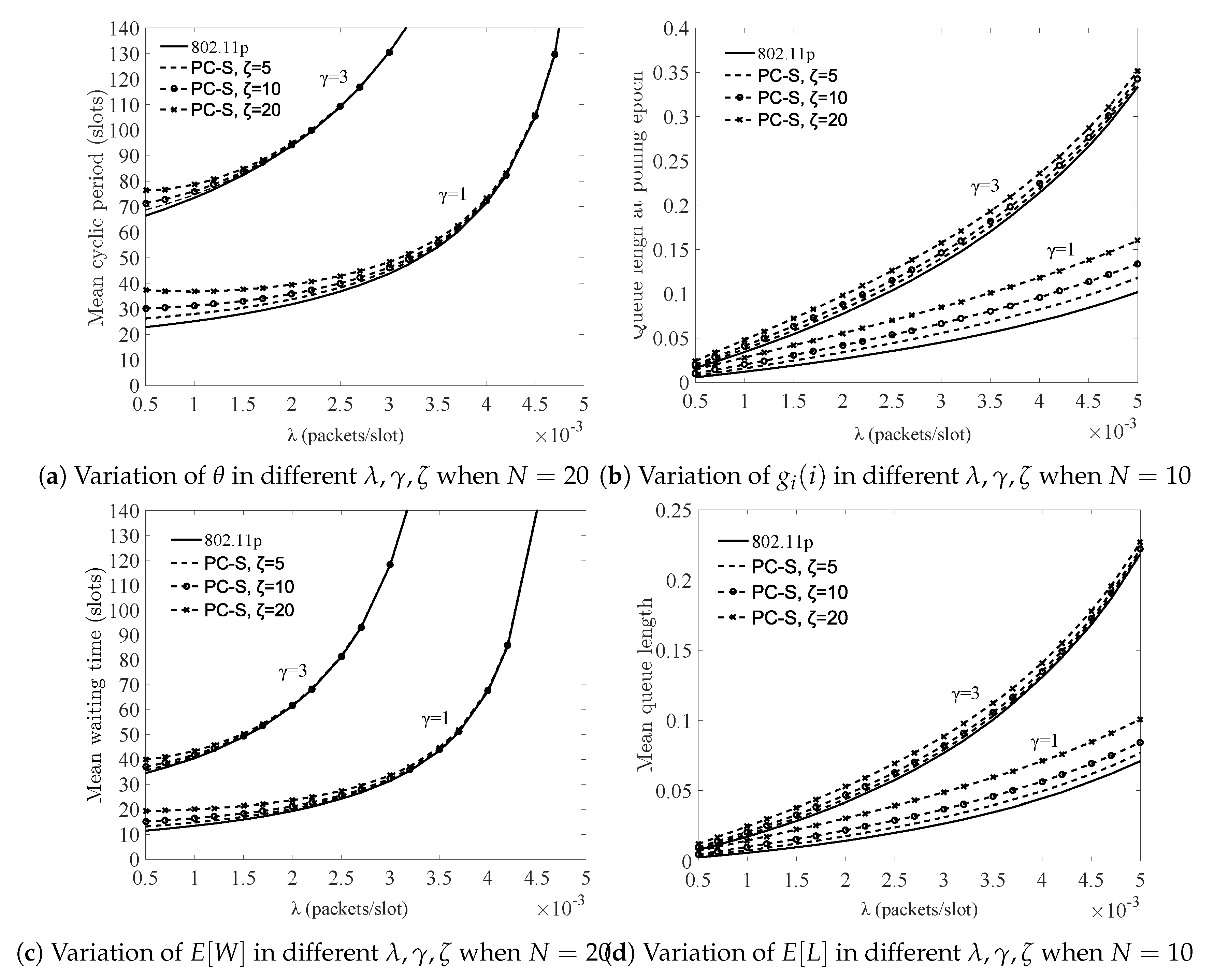
In Figure 4, the variation of $\theta$, $g_i\left(i\right)$, $E[W]$, and $E[L]$ are compared, respectively. It became obvious with the increased traffic load, which clearly showed that the performance of the two systems was degraded and also tended to agree with each other when the load was heavy. Additionally, as shown in Figure 4, the increased switch-over time could result in worse performance, which indicates an unsuitable wireless channel or some distance among the AP and nodes. However, under the stability conditions, $E[W_{PC-S}]$ was only 1 or 2 slots longer than that of 802.11p when $\zeta$ was 5 slots, which means that the QoS could be guaranteed in the PC-S system even if nodes and AP implemented a sleeping strategy when there was no request from the nodes. The reasons are follows:

• AP polls the prior neighbor of the current node according to the polling list, but this neighbor is idle just then. When this case happens, the service moment of the current node will be put off.
• If the AP chooses to turn to sleep while all nodes are sleeping or become DNs, as a result it will not wake up unless the sleeping time ends, even though there are some nodes awakened by the new arrival of packets. However, this is rare in cases of increased load.

Of course, the AP can also choose to keep being active to immediately respond to the critical messages, which will not affect the performance of those sleeping nodes without data.

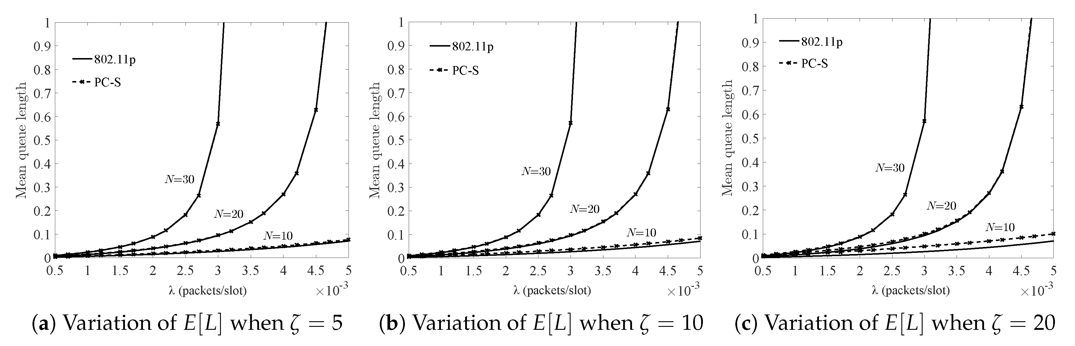
5.2. The Influence of Sleeping Mechanism on the System Performance

Figure 5, Figure 6, Figure 7 and Figure 8 show the change trends of system performance through increasing the nodes under different sleeping factors, arrival rate, and switching-over time. Under the system stability condition, increased load led to worsening of the performance of the two systems. While in case of PC-S system, the influence of the sleeping factor on the system performance was more than that of traffic load when the normalized throughput (i.e., traffic load $\rho =N\lambda \beta$) was under $0.3$. However, when the load increased, it was considered as a key factor.

Additionally, as shown in Figure 5, Figure 6, Figure 7 and Figure 8, in the case of short sleeping time, the sleeping mechanism had a slight influence on the performance degradation in different node scale environments. However, a sleeping factor larger than $\beta +\gamma$ resulted in larger undesirable effects, especially when the throughput $\rho$ was under 0.3.

In Figure 9, the performance variations affected by both $\gamma$ and $\theta$ are compared, and it shows that:

• Under the same service condition, PC-S performed worse than 802.11p. This is because when the traffic load was light, the bigger $\theta$, the worse the performance. However, when load was heavy, the performances under different sleeping factors gradually tended towards those of 802.11p. This is because with increasing load, the probability that all terminals were idle was reduced. Therefore, regardless of the magnitude of the sleeping factor, the probability of the AP passively sleeping was dramatically reduced and the effect of the sleeping mechanism was reduced as well, and ultimately, almost reached zero.
• The effect of $\gamma$ on performance was much greater than the sleeping factor. As shown in Figure 9, even when $\theta$ was as large as 20 slots, the PC-S performance with $\gamma =1$ slot was still much better than that of non-sleeping 802.11p with $\gamma =3$ slots. Therefore, in system design, more attention should be paid to the distance or barriers between terminals and the AP.

5.3. Energy Efficiency Comparisons

In this section, experiments are presented to compare the average sleeping time and energy efficiency, respectively.

5.3.1. The Comparison of Average Node Sleeping Time

The energy consumption in sleeping mode is so low that is ignored. Hence, the energy consumption by a node’s sleeping time can also be evaluated, because under the same condition, the energy consumption of data exchange in these two systems is uniform. Obviously, the longer the idle nodes sleep, the greater the energy efficiency.

In Figure 10, the average sleep time of a node in PC-S under different $\lambda$ and $\theta$ versus the idle time of node in 802.11p is compared.

As shown in Figure 10, the average sleep time of a node in PC-S and the idle time of a node in 802.11p both declined with increasing load. However, when the load was not very heavy, the idle nodes in 802.11p took more than $90\%$ of the time to overhear during the vacation without data transmission. The nodes in PC-S can turn the radio transceivers to sleep in order to reduce the energy consumption. As can be seen in Figure 10b, with increasing $\gamma$ and N, even if the load almost reached the extreme working condition, the sleep rate for PC-S was still about $20\%$.

5.3.2. The Comparison of Average RSU Sleeping Time

The average sleeping time of RSUs under the different arrival rates and sleeping factors when all the nodes were in sleeping mode is shown in Figure 11. For 802.11p, its RSU is always activated, even if the system is idle, so the sleep time is 0 and not shown on the figure.

In Figure 11, it is observed that with increasing sleeping factor under the same conditions, the sleeping time of the RSU became longer but it was shorter than $\zeta$. This is because there were always a few nodes requesting data transmission, and so as long as the traffic load is not zero, the RSU must keep active. Furthermore, increases in the arrival rate and the network scale led to decreases in the RSU’s sleeping time, and finally it dropped down to 0. Especially, when the throughput was more than $0.3$ (i.e., when the system became busy), the RSU’s sleeping time reduced rapidly—even less than 2 slots. Therefore, the RSU can choose to close its sleeping option in order to respond to the nodes quickly. However, this does not mean those idle nodes would remain active, and they can still choose sleeping mode.

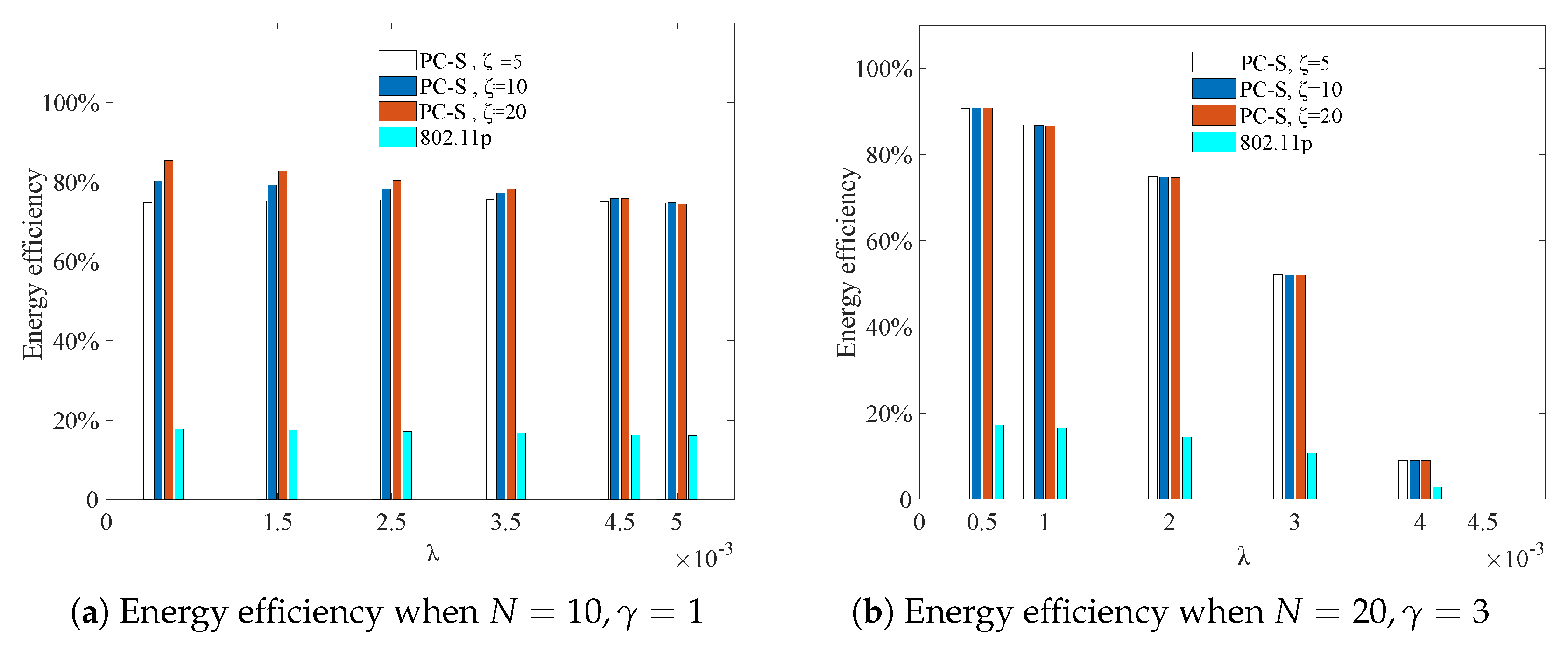
5.3.3. Energy Efficiency Analysis

Unlike 802.11p, when the node in PC-S is idle, it can turn to sleep. So, the saved energy in its sleeping time can be calculated to measure the energy efficiency. If the energy efficiency is denoted by $\eta$, the following equation can be obtained:

$${\eta }_{PC-S}=\frac{E[T_{Slp\_PC-S}]P_i-(E[T_{Slp\_PC-S}]-T_{WS})P_s-T_{SW}{P}_{s2i}}{E[T_{S\_PC-S}]P_t+E[T_{Slp\_PC-S}]P_i+(E[T_{AT\_PC-S}]+E[T_{IBS\_PC-S}])P_r}$$

(14)

where $E[T_{S\_PC-S}]P_t$ is the energy consumption when a node sends its data, $T_{SW}{P}_{s2i}$ is the energy consumption when a node awakens from sleeping state, $E[T_{Slp\_PC-S}]P_i$ is the energy consumption if it keeps idle state during the sleep time, and $(E[T_{AT\_PC-S}]+E[T_{IBS\_PC-S}])P_r$ is the energy consumption of overhearing when it accesses a subnet.

However, the nodes of 802.11p always remain in idle state, even if they have no transmission request. So, the following equation can be obtained:

$${\eta }_P=\frac{E[T_{Idl\_P}]P_r-E[T_{Idl\_P}]P_i}{E[T_{S\_P}]P_t+E[T_{Idl\_P}]P_r+(E[T_{AT\_P}]+E[T_{IBS\_P}])P_r}$$

(15)

where $E[T_{S\_P}]P_t$ is the energy consumption when a node of 802.11p sends its data, $E[T_{Idl\_P}]P_i$ is the energy consumption during its idle state, $E[T_{Idl\_P}]P_r$ is the energy consumption if it keeps overhearing during $E[T_{Idl\_P}]$, and $(E[T_{AT\_P}]+E[T_{IBS\_P}])P_r$ is the energy consumption of overhearing when it accesses a subnet.

In Figure 12, the energy efficiency of a node under different arrival rates and sleeping factors is compared. The variations of energy efficiency when system load was not very high ($N=10,\gamma =1$) is given in Figure 12a. The variations when load was relatively high ($N=20,\gamma =3$) are given in Figure 12b. Thanks to employing the sleeping mechanism, the node in PC-S can save a great deal of energy when it is idle and turns to sleeping mode. However, the node in 802.11p just switches to the idle state from overhearing, which led to only less than $20\%$ energy savings, even when the load was light.

In addition, as shown in Figure 12a, the energy efficiency of PC-S with different $\theta$ came close when load was not high. On the other hand, larger $\theta$ resulted in better energy efficiency performance. However, according to Figure 12b, when $\gamma$ was larger, the improvement of this performance was clearly less with the increment of $\lambda$.

If some packets are lost because of the channel error, the node must retransmit them, which means the arrival rate of the node becomes a little larger than before. Based on Figure 12, the larger $\lambda$, the less energy is saved. Thus, if channel error occurs, the energy efficiency should be reevaluated under the new arrival rate $\lambda$. In this case, the energy efficiency performed more poorly than that of the unaffected system.

5.4. Discussion

All the experiments must be done under normalized stability conditions: $N\lambda (\beta +\gamma )<1$. If the service time and the switch-over time are constant, then the maximum number of nodes in a subnet is calculated as follows:

$$Max\left(N\right)=[\frac{1}{\lambda (\beta +\gamma )}],\lambda ,\beta ,\gamma >0$$

(16)

Obviously, $Max\left(N\right)$ is decreasing with the increment of $\lambda$ after $\beta$ and $\gamma$ adjustment. For example, if $\beta =9$ slots and $\gamma =1$ slot, then the maximum number of nodes in the coverage of a RSU is $Max\left(N\right)=1/10\lambda ,0<\lambda \le 0.1$, which is decided by $\lambda$.

When $N\lambda (\beta +\gamma )\ge 1$, it means the system is oversaturated and ineffective. As a result, the data packets piled up in the nodes will increase in number and the RSU will not be able to transmit them on time> This means that the mean cyclic period, the average waiting time, and the queue length will become enormously high, as shown clearly in Figure 4, Figure 5, Figure 6, Figure 7, Figure 8 and Figure 9.

If the AP chooses to activate the sleeping option on and turns to sleep, it will not wake up until the sleeping time is expired, even if some nodes are awakened by new packet arrivals. Considering the QoS requirement, the sleeping period of the AP should be less than the maximum latency of the packet, which is related to the moving speed, the packet type, etc.

Nevertheless, by introducing the sleeping factor caused by passive vacation, the calculation errors of performance parameters were reduced from more than $9\%$ to almost 0. Experimental results also verified the correctness and effectiveness of the theoretical analysis model.

6. Conclusions

Polling-based proposals in autonomic wireless communication are meaningful when they also consider QoS performance while dealing with energy savings. Towards this end, PC-S appears as the first solution that theoretically addresses sleep state in the system’s mathematical model for the autonomic V2I communication in VANETs and at the same time considers performance. Combined with passive vacation, this paper established a k-limited ($k=1$) analysis model as an expanding protocol that can be used in VANETs for smart cities by employing the embedded Markov chain theory and the probability generating function. For the first time, the exact expressions of first-order and high-order performance characteristics with the sleeping factor were obtained (i.e., the precise expressions of the mean cyclic period, mean waiting time, and mean queue length are achieved). The influence of the sleep mechanism caused by zero-arrival state on the system performances was also analyzed theoretically. Experiments showed that the system model with sleep state caused by the passive vacation of zero-arrival was more suitable for the real scenes than those without zero-arrival state or sleep state. Furthermore, they showed that zero-arrival state and the following sleep state should not be ignored in the theoretical analysis. Meanwhile, compared with IEEE 802.11p, PC-S was more energy-efficient, regardless of whether the load was light or heavy. The longer the sleeping time of a node without data transmission request, the more energy can be saved, and the less electromagnetic interferences from neighbors is, which is an extra benefit of turning off radio transceivers.

Although energy is not the key factor for OBU because it can be easily charged, for those nodes set by roadsides, their energy should be considered carefully. Even if the sleeping option is closed and the OBUs are allowed to keep idle when there are no transmission requests, the suggested mathematical model is still more satisfactory. This is because it pays particular attention to the passive vacation caused by zero-arrival of nodes that often happens, and their precision is verified.

In order to validate the performance of PC-S in some more realistic environments, ongoing work is aimed at implementing PC-S with communication errors involved in the programmable wireless platforms.