Sustainable Integrated Process Planning and Scheduling Optimization Using a Genetic Algorithm with an Integrated Chromosome Representation

Abstract

This paper proposes a genetic algorithm (GA) to find the pseudo-optimum of integrated process planning and scheduling (IPPS) problems. IPPS is a combinatorial optimization problem of the NP-complete class that aims to solve both process planning and scheduling simultaneously. The complexity of IPPS is very high because it reflects various flexibilities and constraints under flexible manufacturing environments. To cope with it, existing metaheuristics for IPPS have excluded some flexibilities and constraints from consideration or have built a complex structured algorithm. Particularly, GAs have been forced to construct multiple chromosomes to account for various flexibilities, which complicates algorithm procedures and degrades performance. The proposed new integrated chromosome representation makes it possible to incorporate various flexibilities into a single string. This enables the adaptation of a simple and typical GA procedure and previously developed genetic operators. Experiments on a set of benchmark problems showed that the proposed GA improved makespan by an average of 17% against the recently developed metaheuristics for IPPS in much shorter computation times.

1. Introduction

A flexible manufacturing system (FMS) is aimed at automated manufacturing by connecting general-purpose facilities such as numerical control machines and machining centers via computer networks and automated logistics systems [1]. The improved flexibility and efficiency of an FMS can allow it to respond rapidly to changes in customer requirements and uncertainties of the manufacturing environments. Process planning is the process of selecting an appropriate process route, machine, tool, and fixtures and jigs for manufacturing a product (part or job). At that time, the part information and specifications, such as shape, materials, and tolerances, must be considered to ensure feasibility and to increase manufacturing efficiency. However, scheduling is the process of determining the temporal schedule of operations to be implemented on each machine so that the entire operation can be performed efficiently with specified manufacturing resources. Process planning and scheduling are the most vital parts of production planning, and their importance is increasing in FMSes due to enhanced flexibility [2].

Process and schedule plans are interrelated. This implies that an optimal schedule does not induce feasible process plans of parts and vice versa. Therefore, their independent planning is inefficient and is also likely to cause feasibility problems. Integrated process planning and scheduling (IPPS) problems are aimed at determining the optimal schedule and a relevant feasible process plan simultaneously. IPPS can consider various alternatives for the process route, operating machine, and required tool. Moreover, it considers constraints such as tool magazine capacity and limitations in the number of available tools. Consequently, the complexity of IPPS is higher than that of flexible job shop scheduling, which belongs to the category NP-complete [3]. Due to the high complexity, traditional approaches for IPPS have preferred solving the two subproblems separately, sequentially, and recursively, rather than solving the subproblems simultaneously. However, recent improvements in computer performance and the availability of numerous metaheuristic approaches have provided useful tools to overcome these limitations. Therefore, there is a growing interest in IPPS for comprehensive planning.

Efficient and feasible planning and execution are essential for manufacturing companies to maximize profits with limited resources. Manufacturing is subject to uncertainties such as equipment failures, order cancellations, design changes, and rush orders [4]. When the uncertainties are pervasive, independent partial optimization in the subproblems can result in long production lead times, increased production costs, delivery delays, infeasible process plans, overloaded operations, and machine failures [5,6]. IPPS, however, can eliminate schedule conflicts, reduce process flow times and work-in-process inventory, and increase utilization and responsiveness to irregular fluctuations. Thus, IPPS can increase the efficiency of manufacturing operations and enhance the competitiveness and sustainability of an enterprise.

IPPS handles various types of flexibilities, such as process, sequence, machine, tool, and tool access direction (TAD) flexibilities [7,8]. Flexibility implies that one of the alternatives can be selected to manufacture a part or implement an operation. Detailed definitions are provided in Section 2. A typical IPPS considers only the process, sequence, and machine flexibility. A few studies have additionally addressed tool and TAD flexibility. However, if a machining center (MC) with an automatic tool changer (ATC) rather than a numerical control machine is a main machine, consideration of the tool flexibility is critical. In addition, most available studies reflect only precedence relation between operations as a constraint. If MCs are utilized, the magazine capacity of the ATC should also be considered [9]. Moreover, as the ATC holds several tools toward the end of the planning period and the number of a particular tool is limited, tool capacity constraint should also be regarded. To our knowledge, Kim et al. [3] has been the only study addressing such tool-related constraints.

Genetic algorithms (GAs) have shown excellent performance for combinatorial problems such as IPPS for a long time. Several GA approaches have also been attempted for IPPS. However, the recent metaheuristics for IPPS have been dominated by ant colony optimization (ACO) and particle swarm optimization (PSO) [8]. To address various flexibilities and properly decode a process plan and schedule, the chromosome of GA must contain information on the operations, process route, sequence of operations, machine, and tool to be processed. It is challenging to combine those attributes into a chromosome because of the difference in their properties. This results in multiple independent chromosomes and, consequently, complex evolution procedures of a GA. Eventually, the solution quality over computation time is lowered.

In this study, we propose a standard GA for solving IPPS, considering tool flexibility and tool-related constraints (hereafter called IPPST). The proposed GA uses a conventional GA procedure and popular genetic operators to increase the convenience of application and to improve the solution quality over the computation time. If the solution quality is remarkable, it is apparent that a straightforward structured algorithm is preferred. To achieve this, we introduced a new integrated chromosome representation, in which a chromosome consists of a permutation of operations, each of which contains fundamental information for scheduling, such as job and operation identifications, the machine and tool identifications to be performed, the related processing time, and the activation indicator. While scheduling, the process route is automatically determined by the sequence order of the relevant operations. By integrating all the information required for scheduling into a chromosome, the evolutionary process is also simplified. Moreover, an identical length of chromosome for all individual renders traditional genetic operators applicable in their present form.

The principal contributions of this paper are summarized as follows. First, this study targets more realistic IPPS. The IPPST we considered is close to realistic manufacturing environments by including the capacity of machines and tools as constraints, which has not been covered by conventional IPPS. Second, this paper proposes a rather efficient metaheuristic of a typical simple GA framework for IPPST optimization. A new and complex approach does not always result in the best results. Even though the approach is typical, more efficiency is better. Simple structured algorithms could be generally easy to implement and robust to environmental differences. Third, this study compares and verifies the performance of various types of metaheuristics with multiple sized IPPST problems. Existing studies have been limited to evaluating specific sample problems and conventional IPPS problems without capacity constraints. In this study, we included performance comparisons of recently developed metaheuristics for IPPST problems composed of 76 to 310 operations.

The paper is organized as follows: Section 2 defines the IPPST and lists the relevant assumptions regarding the manufacturing environment. Section 3 explains the proposed integrated chromosome representation. Section 4 describes genetic operators, fitness function, and the procedure of the GA proposed in this study. In Section 5, the benchmark problems of Kim et al. [3] are introduced, and the experimental results of the proposed GA are compared to those of recently proposed metaheuristics for IPPS. Section 6 and Section 7 provide a discussion of the results of this study and a conclusion and future research directions, respectively.

Notations:

$S$: set of operations that are not assigned

$A$: set of operations that are already assigned

$V$: set of operations that are available for assignment

$i$: job id

$j$: operation id

$o_{i,j}$: jth operation of ith job

$o_{i,j}^{m,t}$: jth operation of ith job with assigned machine m and tool t

$\overleftarrow{o_{l,J}}$: predecessors of $o_{i,j}$

$\overrightarrow{o_{l,J}}$: successors of $o_{i,j}$

$m_{i,j}$: assigned machine id for $o_{i,j}$

$t_{i,j}$: assigned tool id for $o_{i,j}$

$p{t}_{i,j}$: processing time of $o_{i,j}$

$ac{t}_{i,j}$: activation attribute of $o_{i,j}$

$S\backslash \left\{o_{i,j}\right\}$: delete $\left\{o_{i,j}\right\}$ from S

$S\leftarrow \left\{o_{i,j}\right\}$: insert $\left\{o_{i,j}\right\}$ into S

$o_{i,j}\leftarrow S$: pop left-most operation $o_{i,j}$ from S

${\lambda }_{i,j}$: earliest starting time of $o_{i,j}$

${\tau }_{i,j}$: earliest completion time of $o_{i,j}$

${\delta }_m$: earliest starting time of machine m

θ: decision parameter used in hybrid scheduling

$p_{CX}$: probability of crossover

$p_{TS}$: probability of superior selection in tournament selection

$p_{LCM}$: probability of location change mutation

$p_{MTCM}$: probability of machine–tool change mutation

$p_{MTL}$: probability of machine–tool change in each gene

2. Definition and Representation of IPPS

This study considers process, sequence, machine, and tool flexibility [3,7]. Process flexibility implies that alternative process routes can manufacture a feature of a part: A process route is a sequence of operations with precedence relations. Sequence flexibility is the capability to perform the proper process notwithstanding variations in the sequence order of the operations. Machine flexibility refers to the capability where alternative machines can manufacture a feature. Tool flexibility is the capability to process an operation on a machine with alternative tools. Although we do not consider it due to an MC assumption, TAD flexibility refers to the capability to handle an operation with alternative TADs. It applies mainly when the axis of the tool on the machine is fixed and the setup time for the tool change is critical. These flexibilities contribute toward improved mean flow time and machine utilization through efficient process planning and scheduling and also result in an efficient use of bottleneck resources [10].

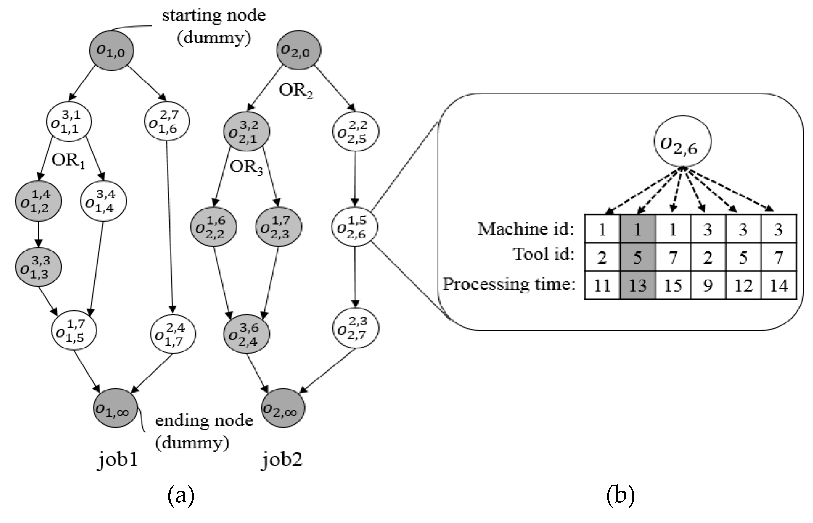
The IPPST can be redefined by modifying Guo et al.’s [11] IPPS definition as follows: “Given a set of $n$ jobs (or parts), each of which has a number of operations, the parts are processed on $m$ machines with alternative manufacturing plans (machines and tools). The objective of the problem is to select suitable manufacturing resources and sequence of the operations so as to determine a schedule wherein the precedence constraints between the operations and resource constraints (tool capacity and tool magazine capacity of each machine) are satisfied and the makespan is minimized.” The most convenient method to describe IPPS involves the use of network representation [12], as shown in Figure 1a. In the graph, each node denotes an operation, and each arrowed line represents the precedence relationship between operations. Operations $o_{i,0}$ and $o_{i,\infty }$ are the starting and ending nodes, respectively, of the $i$th job: These are dummy operations (gray nodes) that are not actually performed. As shown in Figure 1b, each operation consumes a different processing time depending on the machine alternative (machine flexibility) and the tool alternative (tool flexibility). For example, in Figure 1, $o_{2,6}$ can be machined for a specified processing time using one of tools 2, 5, and 7 on one of machines 1 and 3: Machine 1 and tool 5 are selected yielding a processing time of 13 units. Process flexibility can be represented by an OR relationship in Figure 1a. A node with multiple outgoing edges can be an AND node or an OR node, where a node not marked “OR” denotes an AND node. On the AND node, all the operations belonging to the outgoing routes must be performed, whereas on the OR node, the operation belonging to only one selected route is executed. In Figure 1a, all the gray nodes imply dummy operations according to selection of process routes.

We assume the following manufacturing conditions throughout this study:

• All jobs and their network representations are known;
• At the beginning of scheduling, all machines are empty. Thus, any starting operation can be processed from the start time if the assigned machine is available;
• Raw materials are always available;
• Preemption and separation of an operation are not allowed;
• Tools installed in an ATC do not change during the planning period;
• Processing time includes setup time and transportation time;
• Each tool is limited in quantity and is not replenished;
• The number of tool slots in each ATC is fixed, and the number of tool slots consumed depends on the type of tool.

The objective of the IPPS is to minimize the makespan, i.e., the maximum completion time of all jobs.

3. Proposed Chromosome Representation

3.1. Conventional Chromosome Representation

The most important factor that determines the overall procedure and performance of a GA is chromosome representation. As IPPS can be regarded as a job shop scheduling problem (JSP) combined with process, machine, and tool flexibilities, it is common to extend GA representations used in JSP. Cheng et al. [13] classified the types of representation for JSP into direct and indirect according to whether they can directly decode the phenotype from the genotype. Abdelmaguid [14] provided a more rigorous definition, distinguishing the representation types as model-based and algorithm-based depending on the information possessed by the chromosome. The model-based representation constructs chromosomes with decision variables. It can generate a solution directly from the chromosome, and then repairs the infeasibility caused by genetic operations by using a separate repairing algorithm. According to the types of information, it can be further classified into disjunctive graph-based, operation-based, permutation of operations-based, random key-based, preference list-based, and completion time-based. The algorithm-based representation stores the priority rule or order, rather than the decision variables, in the chromosome. It is mainly applied to a constructive-type algorithm such as Giffler and Thompson [15]. There are three types of algorithm-based representation: Priority rule-based, machine-based, and job-based. For a detailed description of the other types, refer to Cheng et al. [13].

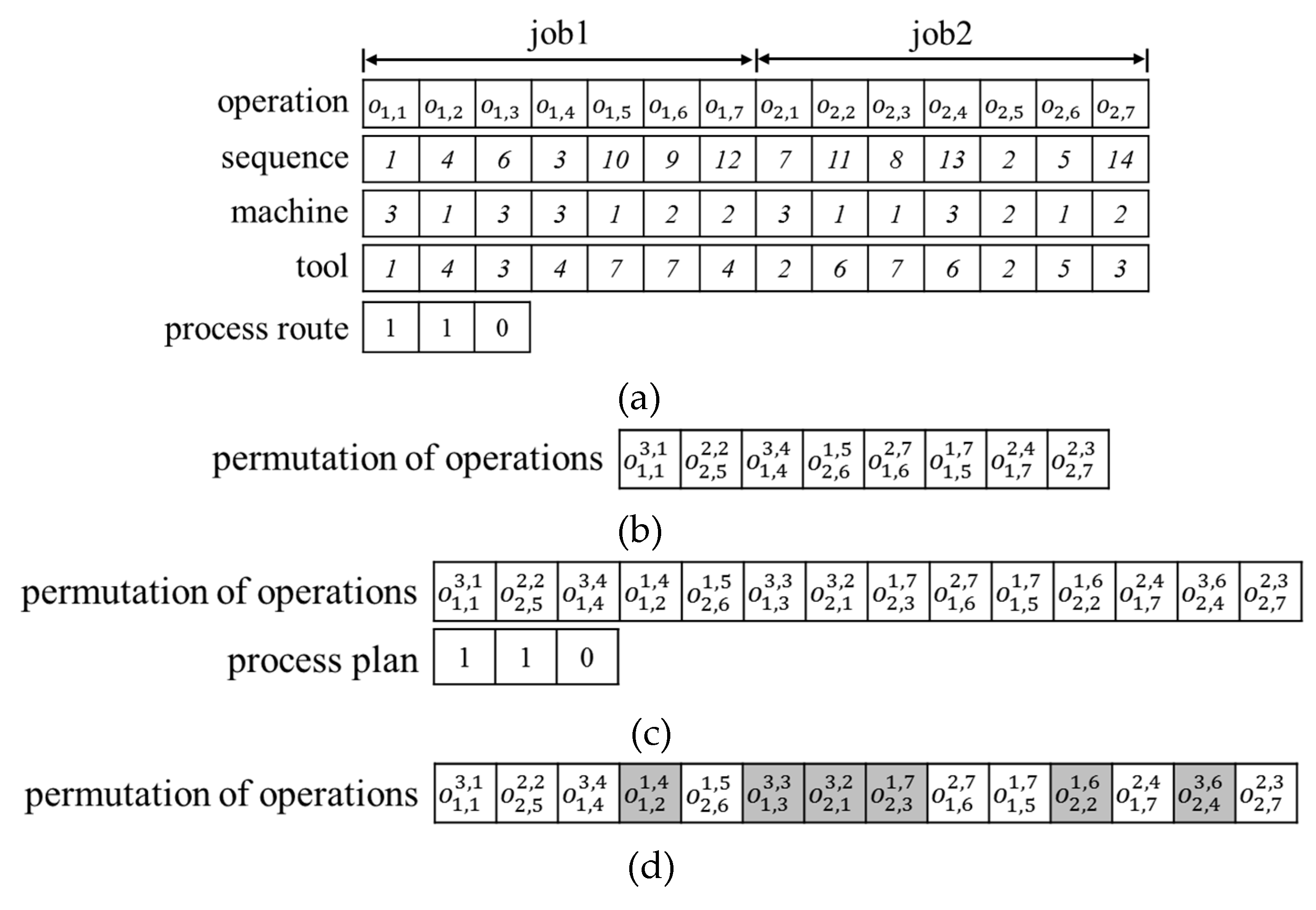
To construct a solution, i.e., a schedule of operations including process plans, IPPS requires information on the sequence of operations, selected process routes, and the machine and tool to be processed in each operation. Therefore, an effective chromosome representation for IPPS must include such information completely. A conventional GA for IPPS prefers an operation-based representation due to its direct interpretation. It consists of several distinct chromosomes, such as sequence of operations, machine identifications (ids), and tool ids, as shown in Figure 2a [8,16,17,18]. Nevertheless, during scheduling, the information from all the chromosomes must be combined and interpreted simultaneously, because the information is interrelated. Moreover, each chromosome evolves independently. It complicates the GA procedure and consumes additional computation time.

Permutation of operations-based representation forms a permutation vector of operations that has all the information required for scheduling. This type is convenient to address: However, it is known to have low exploitation capability. Typical chromosome structures of the permutation of operations-based representation for IPPST (or IPPS) are depicted in Figure 2b,c, where each gene represents an operation and the locus represents the order of the operation. The first type of chromosome representation [19] in Figure 2b consists of only active operations that must be processed depending on the selection of OR relations. The dummy operations are eliminated from the chromosome. For example, the IPPS in Figure 1a can be represented by the structure shown in Figure 2b. The most significant disadvantage of this type of representation is that the length of the chromosome varies according to the selected process routes. Thus, a suitable crossover operator that can address different sizes of chromosome must be provided. The second type [3,20], in Figure 2c, retains two distinct chromosomes: An operation string and a process plan string. The operation string is composed of all the operations in the IPPS network, and each operation has information on job id, operation id, machine id, and tool id. The process plan string has information on the selected process routes. There are several formations on the process plan string: However, here, we will describe a straightforward binary string as an example. In Figure 1a, job 1 has an OR node, and job 2 has two OR nodes. Suppose that the binary process plan string has a length equivalent to the number of OR nodes in the IPPS network and that the value of a gene is 0 for the left route and 1 for the right route. In Figure 1a, the right one is selected in OR₁, and the right and left routes are selected in OR₂ and OR₃, respectively. Therefore, the process plan string on the right side of Figure 2b becomes 1, 1, and 0. The dummy operations on the unselected routes are determined by the process plan string during scheduling according to decision rules, as shown in Figure 3b. This type of representation has a fixed chromosome length for an IPPS. It enables the conventional genetic operators applicable. However, it requires an independent evolution process for each chromosome and additional computation to determine the dummy operations during scheduling.

3.2. Integrated Chromosome Representation

In this paper, we propose a new type of chromosome representation (Figure 2d), namely integrated chromosome representation (ICR). As it includes all the operations of an IPPS network, the length of the chromosome is a constant. Each gene contains all five attributes required for scheduling, as shown in Figure 3a: Job id, operation id, machine id, tool id, and activation. As the remaining attributes can be conveniently inferred from the name, we explain only the activation attribute. It is a Boolean variable that indicates whether the operation should be performed. If it is true (white cell in Figure 2d), the operation is active. Otherwise (gray cell in Figure 2d), it is inactive, i.e., a dummy operation. The structure resembles that of the second type of the permutation of operations-based representation: However, it operates in a completely different manner. The key concept is to use the order of operations as a selection rule for process routes in OR relations, as shown in Figure 3b, rather than a separate process plan string. At the beginning of decoding, all the activation attributes in all the operations are set as true. During the decoding, if the first operation in a subroute under OR relation is located toward the left of one of the complementary subroutes, the subroute is selected as the process plan. Then, all the operations belonging to the complementary subroutes are deactivated. For example, in OR₁ of Figure 1a, subroutes $o_{1,4}$ and $o_{1,2}-o_{1,3}$ are in an OR relation. Therefore, the order of $o_{1,4}$ and $o_{1,2}$ is important. In the chromosome in Figure 2d, $o_{1,4}$ is ahead of $o_{1,2}$: Therefore, the route $o_{1,4}$ is selected as the process plan and the operations $o_{1,2}$ and $o_{1,3}$ are deactivated as dummy nodes. Similarly, for OR₂ of Figure 1a, as the order of $o_{2,5}$ precedes $o_{2,1}$ in the chromosome, the activation status of $o_{2,5}$, $o_{2,6}$, and $o_{2,7}$ are maintained as active, and the operations $o_{2,1}$, $o_{2,2}$, $o_{2,3}$, and $o_{2,4}$ in the complementary subroute become dummy nodes. In OR₃, all the operations in the subroutes are already inactive: Therefore, the selection procedure is skipped.

Using ICR, the process plan and the schedule plan (in case of the use of semi-active scheduling) can be represented in a chromosome. In the example in Figure 2, the process plan becomes $o_{1,1}-o_{1,4}-o_{1,6}-o_{1,5}-o_{1,7}$ for job 1 and $o_{2,5}-o_{2,6}-o_{2,7}$ for job 2. The schedule of each operation is determined from the left to the right sequentially by semi-active scheduling. In addition, ICR requires a chromosome for an individual, and therefore, only an evolution procedure is necessary. It simplifies the structure of GA and consequently results in a shorter computation time. The same chromosome length also facilitates the development of new genetic operators and enables the adoption of conventional operators without modification. To decrease the computation time further, the pair information on the complementary subroutes can be stored in a separate repository in advance and can be retrieved on demand. This is because all the feasible alternative process subroutes in OR relations are determined by process engineers prior to the execution of IPPS.

4. GA Procedures

4.1. Decoding Methods

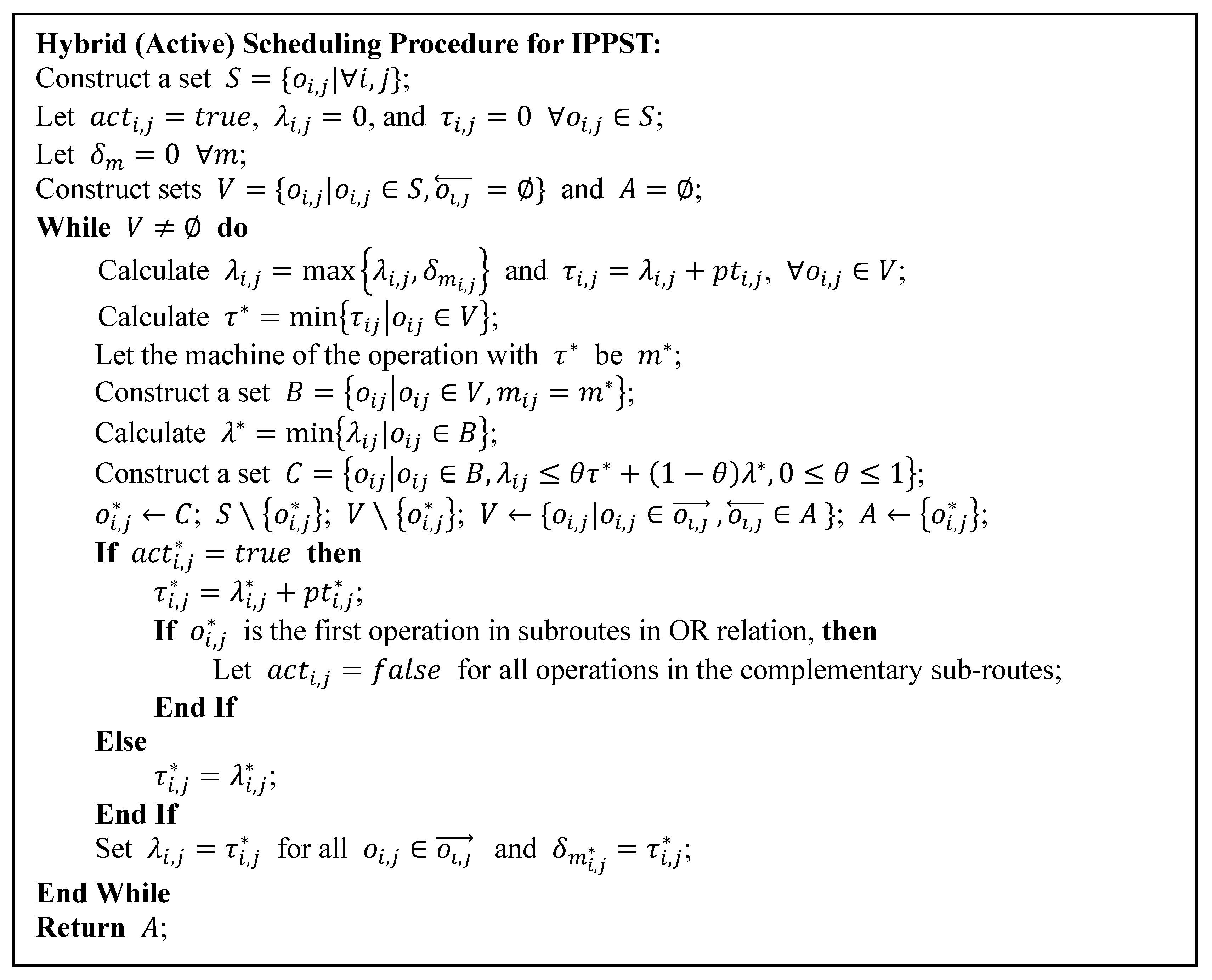
The ICR directly describes process plans: However, the final schedule must be decoded from the chromosome by a scheduling algorithm. It is well known that the optimal schedule is an active schedule in JSP and, consequently, IPPS and IPPST. The most popular active scheduling algorithms are Giffler–Thompson [15] and the hybrid scheduling algorithm [3,21], as shown in Figure 4.

Those active scheduling algorithms generally provide significantly more effective solutions than those by a straightforward semi-active scheduling, as shown in Figure 5. However, from the perspective of computational efficiency, they are not always superior, particularly in GAs for IPPST. Active scheduling includes numerous search procedures, as shown in Figure 4. Therefore, it consumes substantial computation time compared to semi-active scheduling. If the number of candidate operations for the next operation is large, such as in IPPST, the computation time increases rapidly.

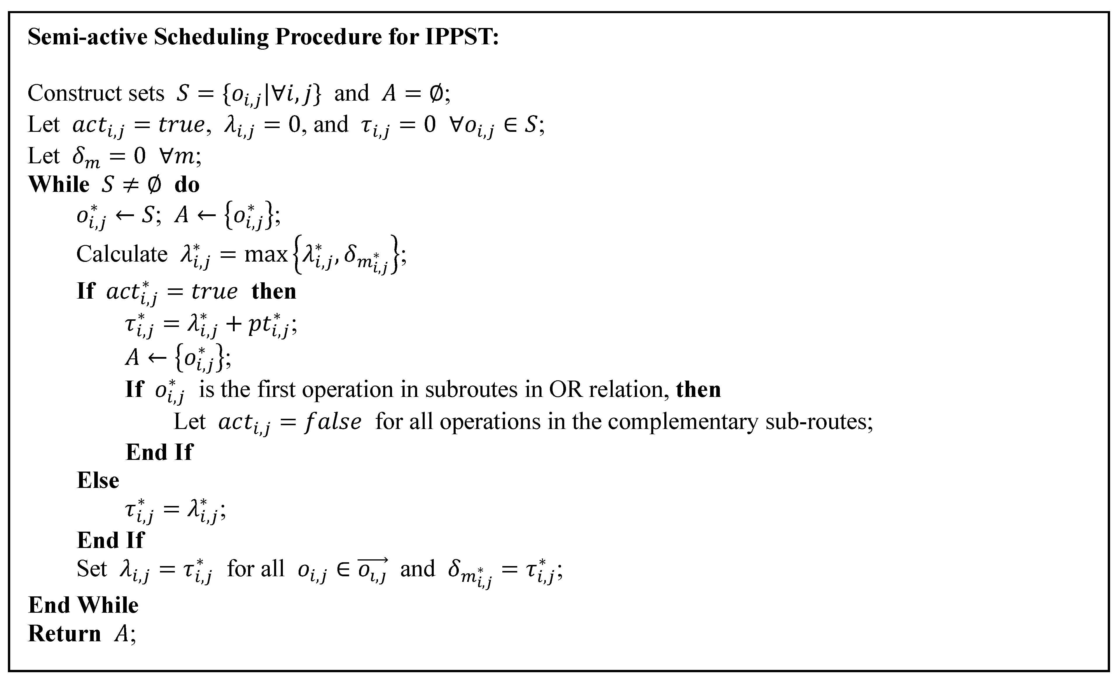
More importantly, active (or hybrid) scheduling does not utilize the information on a sequence of operations. As shown by the procedure in Figure 4, active scheduling completely disassembles the sequence of operations and reassigns it to the schedule according to precedence relation and the assignment rules. It implies that the inheritance characteristic of GA diminishes in active scheduling, as Shi [22] has indicated. For example, consider two chromosomes that are composed of the same operations and only whose sequences are different. Then, active scheduling generates almost identical schedules for both the chromosomes. A crossover operation of the two individuals is also ineffective because it only changes the sequence of operations. This reduces diversification and degrades the performance of the GA. However, semi-active scheduling can improve the quality of solution by a crossover operation if it is effective because it inherits an important partial sequence. To summarize, in the GA that utilizes active scheduling as a decoder, the optimization of the process plan is performed by the GA, and the optimization of the schedule is performed by the active scheduling. However, in a GA using semi-active scheduling as a decoder, the optimization of both the process plan and schedule is managed by the GA, and semi-active scheduling serves only as a pure decoder. For these reasons, in the main procedure of the proposed GA, we adopted semi-active scheduling to increase computational efficiency.

4.2. Fitness Function

The most popular objective function is a makespan, so we employed the inverse of makespan as a fitness function. In IPPST, however, the penalties on constraints on tool magazine capacity and tool capacity should be considered. In this study, we adopted the fitness function of Kim et al. [3] with a marginal modification, which adds penalties to the violation of the constraints. Fitness is calculated by Equation (1):

$$\mathrm{fitness}=\frac{100,000}{\mathrm{makespan}+c_1{{\displaystyle \sum }}_t{\left[2TP\left(t\right)\right]}^{\alpha }+c_2{{\displaystyle \sum }}_m{[2MP\left(m\right)]}^{\beta }}$$

(1)

Here, $TP\left(t\right)$ is the tool capacity penalty, indicating the excess amount of tool $t$ over the tool capacity, and $MP\left(m\right)$ is the tool magazine capacity penalty, indicating the number of overused slots relative to the tool magazine capacity of machine $m$. If both the penalties do not exceed the capacities, they are zeros. In addition, $c_1,c_2,\alpha ,$ and $\beta$ are the parameters that determine the magnitude and the degree of the penalties. Several preliminary tests revealed that the fitness function of Kim et al. [3] derived infeasible solutions for large-sized problems. Thus, we modified it as Equation (1) by multiplying two on $TP\left(t\right)$ and $MP\left(m\right)$ in the original one. The coefficients $\left(c_1,c_2,\alpha ,\beta \right)$ were also changed from (10, 10, 0.5, 0.5) to (200, 200, 2, 2) for the same purpose.

4.3. Overall GA Procedure

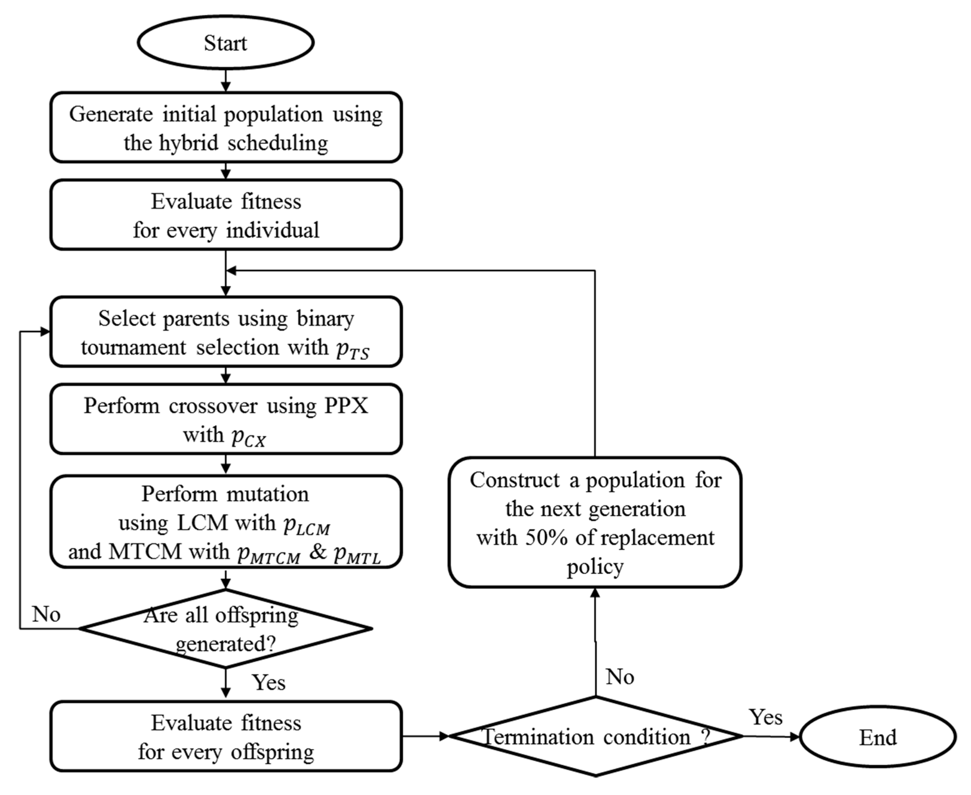
The proposed GA follows the typical GA procedure, as shown in Figure 6. In the beginning, a certain number of precedence-preserved individuals are generated as an initial population by using the hybrid scheduling in Figure 4. At the end of each generation, fitness evaluation for all individuals is performed. Reproduction follows the conventional selection–crossover–mutation procedures. The proposed GA uses binary tournament selection for reproduction to increase diversification, wherein a superior individual is selected if a random number is less than or equal to $p_{TS}$, and an inferior individual is selected if the number is larger than $p_{TS}$. In crossover, the precedence-preservative crossover (PPX) is executed for the selected parents with a probability of $p_{CX}$. The generated offspring is applied with a location change mutation (LCM) with a probability of $p_{LCM}$. It moves the locus of a randomly selected operation while satisfying precedence relations. Then, the offspring is applied with a machine–tool change mutation (MTCM) with a probability of $p_{MTCM}$. In the procedure, the machine and tool of randomly selected operations with $p_{MTL}$ are replaced by a machine and tool inducing a minimal processing time. The next generation is constructed as follows: 50% of individuals with good solutions in the population survive, and the rest are replaced by superior solutions in the offspring. A termination condition is a number of generations. Detailed procedures will be described in the following subsections.

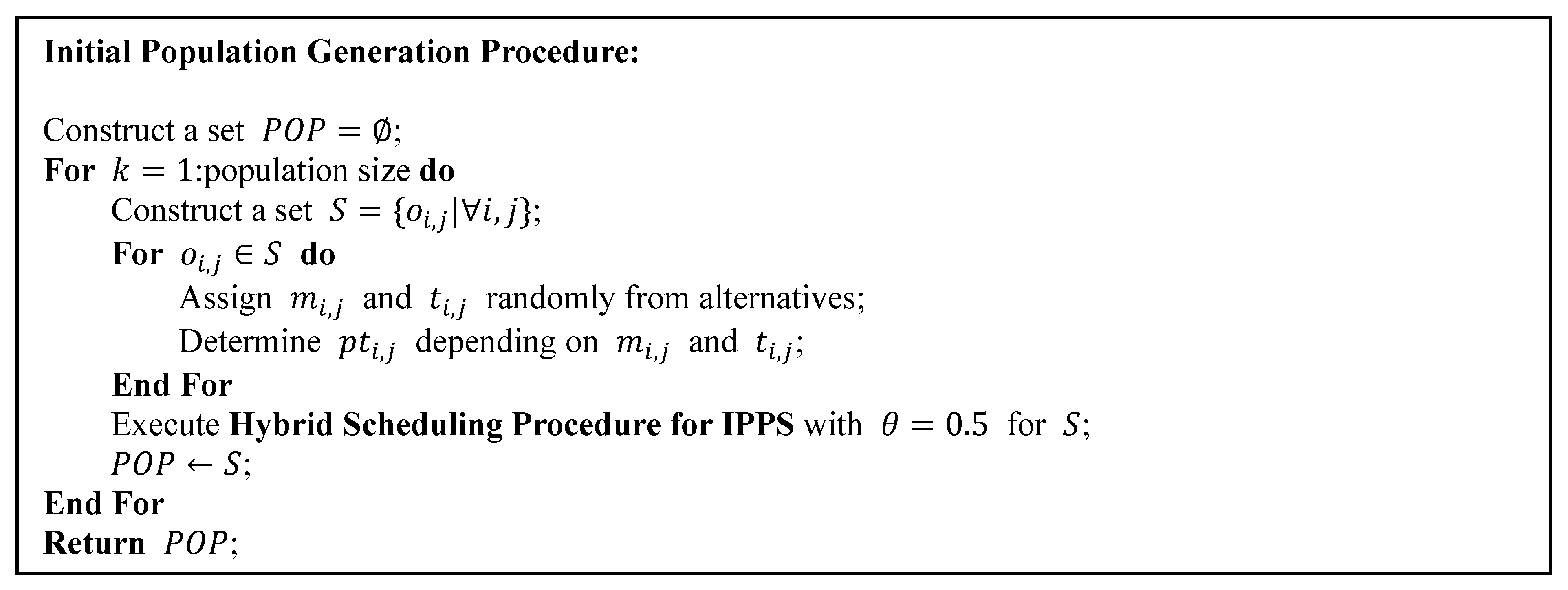
4.4. Generation of Initial Population

The initial population affects the quality of the solution. Although the proposed GA uses a semi-active scheduling as a main decoder, the hybrid scheduling in Figure 4 is adopted for generating the initial population to obtain more effective initial solutions, as shown in Figure 7.

4.5. Crossover Operation

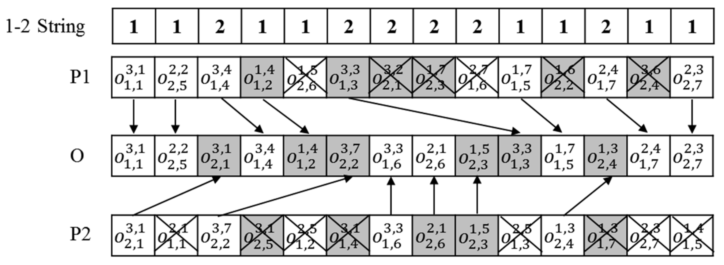
Because the proposed GA uses semi-active scheduling as a decoder, the precedence relationship among the operations in the chromosome must be retained always. Hence, we adopted the PPX of Bierwirth and Mattfeld [21] for a crossover. Although the procedure of PPX is popular, we describe it via the example of Figure 8. If a random number is larger than $p_{CX}$, a string composed of one or two is generated arbitrarily with an identical length to the individual chromosome. Starting from the first element, if the value is one, the first operation of P1 (P2 if two) is copied to the leftmost empty gene of the offspring (O), and the operation with identical job and operation ids is deleted from the parents (P1 and P2). This process is repeated until all the operations are assigned to the offspring.

4.6. Mutation Operation

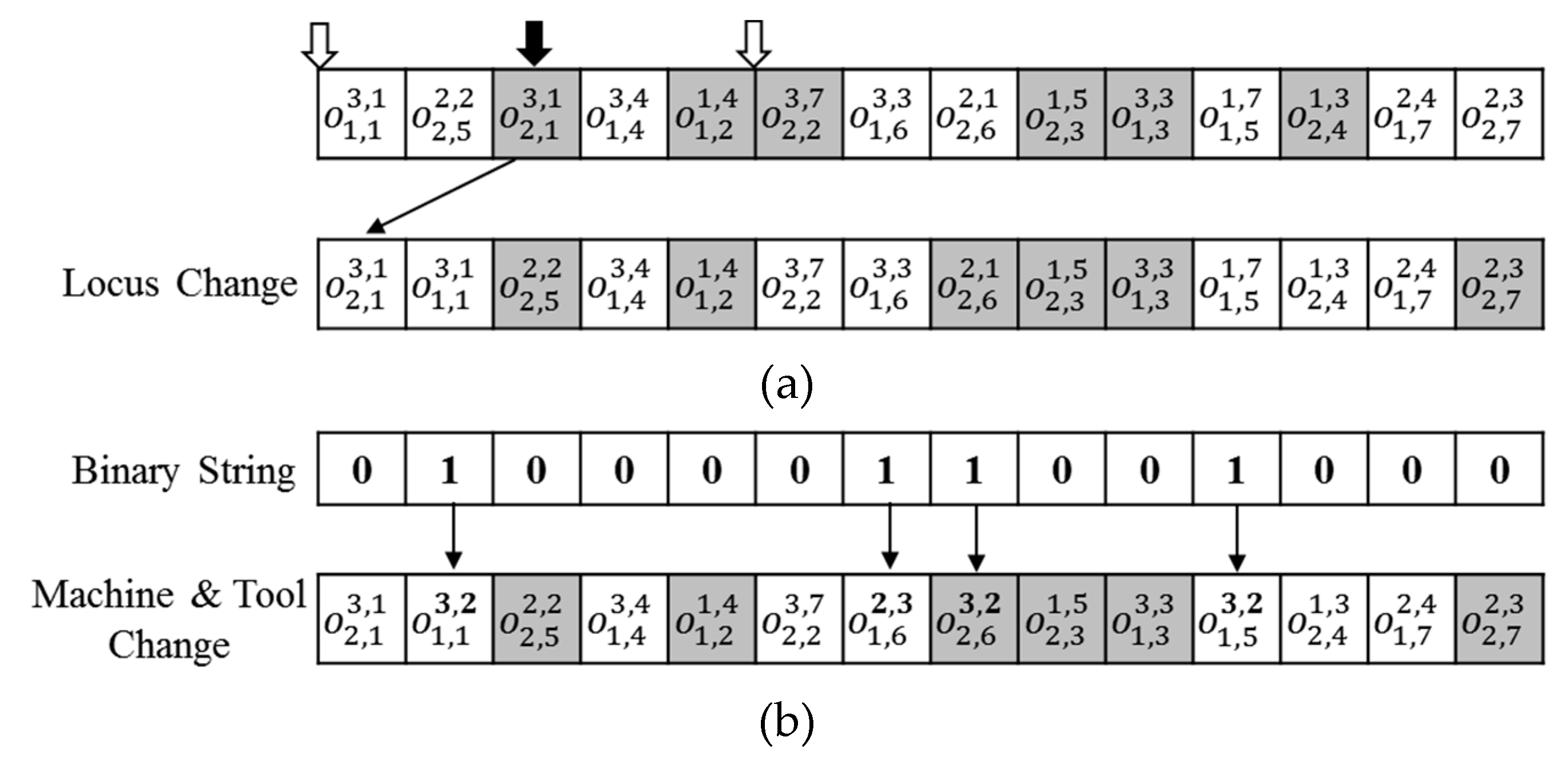
Mutation is an important genetic operator to enhance diversification of GA. The typical mutation operation is to change the locus of a selected gene. Thus, we employed an LCM (location change mutation), as shown in Figure 9a. First, an operation ($o_{2,1}^{3,1}$, black-arrowed gene) is randomly selected, and the loci are changed arbitrarily to the first locus. At this time, to retain the precedence relationship, the permissible range of loci (within white arrows) is restricted between the predecessor ($o_{2,0}$ or nothing) and successors ($o_{2,2}^{3,7}$ and $o_{2,3}^{1,5}$) of the operation $o_{2,1}^{3,1}$. If the ICR is adopted, LCM can change the selected process route as well as the sequence of operations. Note that the dummy operations are also changed in Figure 9a.

Though LCM increases intensification of GA well, our preliminary experiments revealed that the improvement of solution quality was unsatisfiable due to the large solution space of IPPST. Therefore, we adopted another mutation operator, namely, MTCM (machine–tool change mutation). It increases the intensification capability of GA and therefore helps to improve solution quality even with a reasonable size of population. The fundamental concept of MTCM is to change the machine and tool of an operation into the combination that induces the minimal processing time. The detailed procedure is illustrated in the example of Figure 9b. First, a random binary string of the length of the chromosome is generated, in which the number of ones is the largest integer less than or equal to $p_{MTL}$ times the chromosome length. Then, at each gene, if the value is one, the machine and the tool are reassigned as the machine and tool set of the minimal processing time: Otherwise, the existing assignments are retained. For instance, the minimal processing time 9 of $o_{2,6}$ is derived from machine 3 and tool 2, as shown in Figure 1b. Thus, $o_{2,6}^{2,1}$ is changed into $o_{2,6}^{3,2}$ in Figure 9b.

The factors that significantly influence the schedule in IPPST are the sequence of operations, the selected process route in OR relations, and the machine and tool to be processed. LCM changes the sequence of operations and the selected process route. On the other hand, MTCM changes the machine and tool. Machine change can be effective in reducing the idling time between operations because it changes the starting time of the operation and distributes the resources. Particularly, a change in the early period affects all the subsequent schedules. Tool change only changes the processing time of the operation. However, changes in machine and tool influence the feasibility of the solution due to the constraints.

5. Benchmark Problems and Experimental Environment

For the performance evaluation of the proposed GA, the set of problems of Kim et al. [3] was selected as a benchmark. The problems are well defined and also have the advantage of being convenient to compare to available results. In fact, most IPPS studies that do not consider tool flexibility and tool-related constraints use Kim et al.’s [3] problem set as a benchmark. As shown in

Table 1. Benchmark problems for IPPST.

Problem	#ops	Job Number	Problem	#ops	Job Number
P1	89	1, 2, 3, 10, 11, 12	P16	160	2, 3, 6, 9, 11, 12, 15, 17, 18
P2	100	4, 5, 6, 13, 14, 15	P17	155	1, 2, 4, 7, 8, 12, 15, 17, 18
P3	121	7, 8, 9, 16, 17, 18	P18	155	3, 5, 6, 9, 10, 11, 13, 14, 16
P4	99	1, 4, 7, 10, 13, 16	P19	159	4, 5, 6, 7, 8, 9, 10, 11, 12
P5	102	2, 5, 8, 11, 14, 17	P20	151	1, 2, 3, 13, 14, 15, 16, 17, 18
P6	109	3, 6, 9, 12, 15, 18	P21	189	1, 2, 3, 4, 5, 6, 10, 11, 12, 13, 14, 15
P7	103	1, 4, 8, 12, 15, 17	P22	221	4, 5, 6, 7, 8, 9, 13, 14, 15, 16, 17, 18
P8	96	2, 6, 7, 10, 14, 18	P23	201	1, 2, 4, 5, 7, 8, 10, 11, 13, 14, 16, 17
P9	111	3, 5, 9, 11, 13, 16	P24	211	2, 3, 5, 6, 8, 9, 11, 12, 14, 15, 17, 18
P10	105	4, 5, 6, 10, 11, 12	P25	199	1, 2, 4, 6, 7, 8, 10, 12, 14, 15, 17, 18
P11	76	7, 8, 9, 13, 14, 15	P26	207	2, 3, 5, 6, 7, 9, 10, 11, 13, 14, 16, 18
P12	105	1, 2, 3, 16, 17, 18	P27	205	4, 5, 6, 7, 8, 9, 10, 11, 12, 13, 14, 15
P13	142	1, 2, 3, 5, 6, 10, 11, 12, 15	P28	212	1, 2, 3, 7, 8, 9, 13, 14, 15, 16, 17, 18
P14	168	4, 7, 8, 9, 13, 14, 16, 17, 18	P29	262	2, 3, 4, 5, 6, 8, 9, 10, 11, 12, 13, 14, 16, 17, 18
P15	150	1, 4, 5, 7, 8, 10, 13, 14, 16	P30	266	1, 4, 5, 6, 7, 8, 9, 11, 12, 13, 14, 15, 16, 17, 18
P31	310	1, 2, 3, 4, 5, 6, 7, 8, 9, 10, 11, 12, 13, 14, 15, 16, 17, 18

, the total number of benchmark problems is 31, and each problem consists of a subset of 18 jobs (parts), as shown in

Table 2. Job description of the benchmark problem for IPPST.

Job id	#ops	#ORs	Job id	#ops	#ORs	Job id	#ops	#ORs
1	12	2	7	21	4	13	18	3
2	14	1	8	20	4	14	13	2
3	19	2	9	20	3	15	15	2
4	16	2	10	11	1	16	21	3
5	18	2	11	15	2	17	22	4
6	20	2	12	18	2	18	17	3

. Each job consists of 12–22 operations (#ops) with precedence relations, and the number of OR nodes (#ORs) is 1–4. The number of operations (#ops) for each problem varies from 76 to 310.

The facility has machine magazine capacity and tool capacity, as mentioned in Section 2. There are in total 10 machining centers, and each machine operates a magazine with 26–38 tool slots, as shown in

Table 3. Magazine capacity and tool capacity of the benchmark problems.

Magazine Capacity		Tool Capacity
Machine id	#Slots	Tool id	#Copies	#Required Slots	Tool id	#Copies	#Required Slots
1	28	1	6	1	11	7	1
2	31	2	7	2	12	10	2
3	38	3	6	2	13	9	3
4	28	4	6	2	14	8	2
5	36	5	10	1	15	6	2
6	37	6	6	2	16	10	2
7	29	7	10	3	17	9	1
8	28	8	9	2	18	6	2
9	29	9	7	1	19	8	2
10	26	10	5	2	20	7	3

. There are 20 types of tools, each of which exhibits a certain quantity: The number of slots required in the magazine varies according to each tool.

The proposed GA was implemented using Julia language version 1.0, which is a recently introduced programming language based on a low-level virtual machine (LLVM) just-in-time (JIT) complier. The experiment was performed on an Intel^® Core™ i7-6700U [email protected] GHz with 16 GB memory. The computation time was measured by CPU time in seconds.

6. Experimental Results

6.1. Determination of Operating Parameters

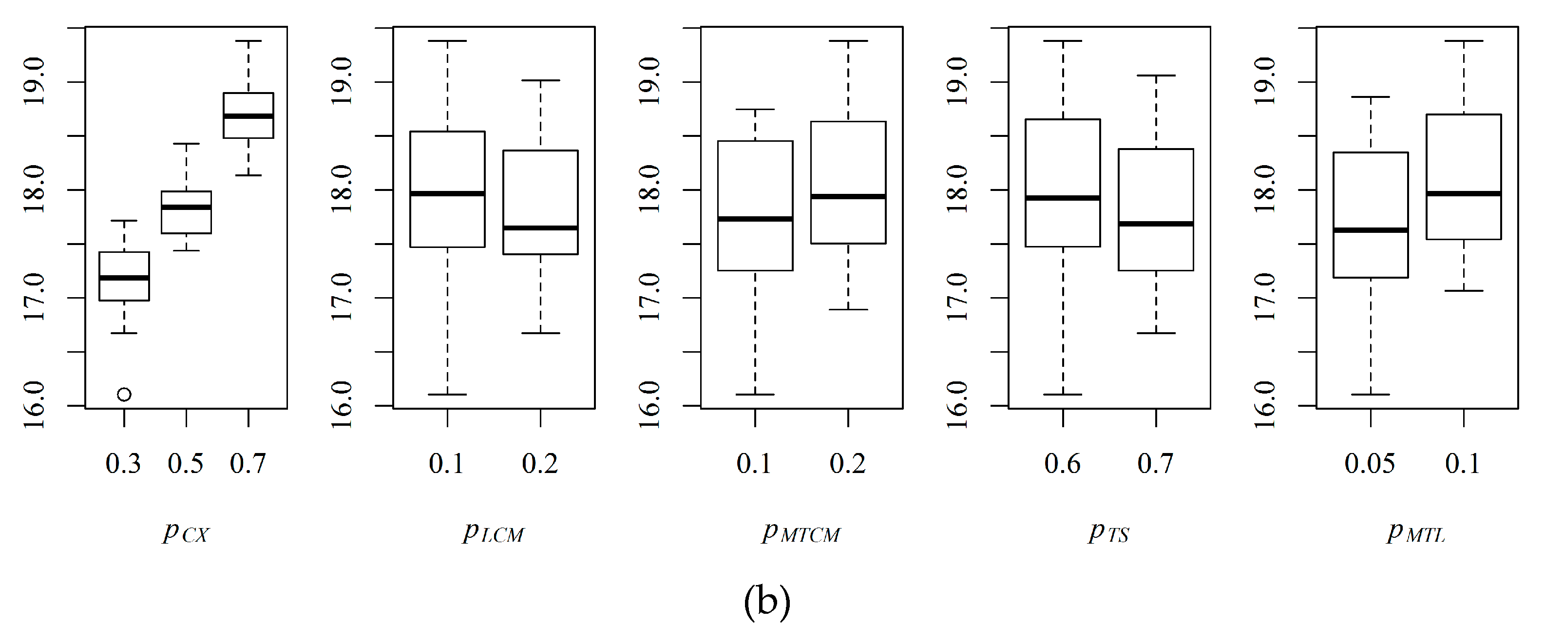
A preliminary test was performed to determine the parameters $p_{CX}$, $p_{LCM}$, $p_{MTCM}$, $p_{TS}$, and $p_{MTL}$. Two or three levels were assigned to each parameter. The experimental conditions were as follows: The selected problems were P1, P13, P21, P29, and P31; the number of repetitions was 10 for each treatment; the population size was 50; and the number of generations was 1000.

Table 4. Average makespan according to operating parameters for the five selected problems.

${\mathit{p}}_{\mathit{C}\mathit{X}}$	${\mathit{p}}_{\mathit{L}\mathit{C}\mathit{M}}$	${\mathit{p}}_{\mathit{M}\mathit{T}\mathit{C}\mathit{M}}$	${\mathit{p}}_{\mathit{T}\mathit{S}}$	${\mathit{p}}_{\mathit{M}\mathit{T}\mathit{L}}$	$\overline{{\mathit{C}}_{\mathit{m}\mathit{a}\mathit{x}}}$							$\mathsf{\Sigma }\overline{{\mathit{t}}_{\mathit{comp}}}$
					P1	P13	P21	P29	P31	$\mathsf{\Sigma }\overline{{\mathit{C}}_{\mathit{m}\mathit{a}\mathit{x}}}$	Rank
0.3	0.1	0.1	0.6	0.05	177.9	214.5	290.1	389.7	449.0	1521.2	41	16.1
				0.10	168.2	209.2	274.5	365.3	482.2	1499.4	34	17.38
			0.7	0.05	188.1	211.1	284.8	369.9	463.1	1517.0	40	16.98
				0.10	171.7	210.8	279.7	355.1	455.4	1472.7	23	17.12
		0.2	0.6	0.05	169.4	210.8	282.0	359.2	453.0	1474.4	26	17.39
				0.10	170.3	199.5	270.4	358.3	454.3	1452.8	16	17.72
			0.7	0.05	172.9	208.9	278.9	370.6	421.1	1452.4	15	17.13
				0.10	176.2	204.4	274.9	366.0	442.3	1463.8	21	17.72
	0.2	0.1	0.6	0.05	172.2	209.7	274.7	379.0	473.0	1508.6	36	16.97
				0.10	170.2	197.2	280.8	358.0	426.3	1432.5	6	17.49
			0.7	0.05	177.4	209.3	285.0	379.7	461.9	1513.3	39	16.68
				0.10	167.4	203.1	266.5	357.3	463.5	1457.8	19	17.06
		0.2	0.6	0.05	172.2	212.0	269.8	347.7	426.9	1428.6	5	17.24
				0.10	170.1	200.9	263.3	366.2	465.3	1465.8	22	17.46
			0.7	0.05	169.3	205.2	280.7	358.7	424.1	1438.0	9	16.89
				0.10	171.1	199.3	275.3	352.1	445.6	1443.4	13	17.37
0.5	0.1	0.1	0.6	0.05	177.5	227.3	297.2	367.9	461.3	1531.2	45	17.81
				0.10	169.6	208.8	279.1	371.8	482.4	1511.7	37	17.99
			0.7	0.05	177.4	209.1	292.4	372.9	473.9	1525.7	42	17.66
				0.10	169.6	206.7	290.3	357.1	449.8	1473.5	24	17.95
		0.2	0.6	0.05	177.0	210.6	286.4	350.3	472.3	1496.6	33	17.99
				0.10	171.5	206.3	271.0	363.9	428.1	1440.8	11	18.43
			0.7	0.05	175.2	202.7	289.8	385.3	458.9	1511.9	38	17.55
				0.10	173.7	206.7	278.3	351.3	428.8	1438.8	10	18.31
	0.2	0.1	0.6	0.05	175.8	219.7	282.5	368.4	455.2	1501.6	35	17.58
				0.10	170.1	210.3	275.0	353.0	428.3	1436.7	7	17.87
			0.7	0.05	172.7	216.0	284.6	369.3	451.4	1494.0	32	17.44
				0.10	172.2	213.7	271.6	351.8	436.0	1445.3	14	17.60
		0.2	0.6	0.05	174.3	213.1	278.0	345.2	426.8	1437.4	8	17.70
				0.10	169.3	205.1	261.4	358.4	410.7	1404.9	3	18.28
			0.7	0.05	169.6	201.2	280.5	347.4	443.1	1441.8	12	17.60
				0.10	169.1	202.1	268.8	347.0	418.1	1405.1	4	17.89
0.7	0.1	0.1	0.6	0.05	172.4	215.8	296.8	391.4	496.3	1572.7	48	18.50
				0.10	171.5	212.4	281.3	346.1	475.4	1486.7	31	18.75
			0.7	0.05	186.5	223.9	300.2	373.5	450.9	1535.0	46	18.46
				0.10	171.0	212.3	278.4	363.8	501.8	1527.3	43	18.71
		0.2	0.6	0.05	180.3	219.7	290.2	361.0	428.4	1479.6	29	18.86
				0.10	174.4	203.7	270.8	378.0	447.0	1473.9	25	19.38
			0.7	0.05	173.6	211.8	282.6	365.7	448.8	1482.5	30	18.59
				0.10	172.3	202.2	274.8	357.5	448.4	1455.2	18	19.06
	0.2	0.1	0.6	0.05	178.5	226.1	287.5	370.1	467.3	1529.5	44	18.63
				0.10	174.5	211.4	274.2	361.6	457.3	1479.0	28	18.69
			0.7	0.05	177.4	223	292.5	390.5	470.6	1554.0	47	18.14
				0.10	170.2	206.4	270.4	355.6	461.0	1463.6	20	18.45
		0.2	0.6	0.05	174.5	212.2	275.4	368.1	445.5	1475.7	27	18.68
				0.10	168.9	196.7	264.2	341.5	424.0	1395.3	1	19.02
			0.7	0.05	170.1	205.4	267.2	360.7	450.8	1454.2	17	18.24
				0.10	170.9	208.9	262.3	347.4	409.1	1398.6	2	18.94
average					173.3	209.5	278.9	363.0	450.3	1475.0		17.90
standard deviation					4.3	7.0	9.4	12.2	21.1	41.0		0.70

shows the experimental results of the average makespan ($\overline{C_{max}}$) and the sum of the average computation time ($\mathsf{\Sigma }\overline{t_{comp}}$) according to the level of parameters for the five selected problems, where the last column of $\overline{C_{max}}$ is the rank of the sum of $\overline{C_{max}}$ ($\mathsf{\Sigma }\overline{C_{max}}$) in ascending order. Figure 10ab shows the boxplots of $\mathsf{\Sigma }\overline{C_{max}}$ and $\mathsf{\Sigma }\overline{t_{comp}}$ depending on the level of the five parameters.

In Figure 10, $p_{CX}$ only affected computation time critically, while the remaining parameters affected both makespan and computation time. To confirm the effects of each parameter, a Kruskal–Wallis test was performed on $\mathsf{\Sigma }\overline{C_{max}}$ and $\mathsf{\Sigma }\overline{t_{comp}}$, and the results are summarized in

Table 5. Kruskal–Wallis test results for $\Sigma \overline{{\mathit{C}}_{\mathit{max}}}$ and $\Sigma \overline{{\mathit{t}}_{\mathit{comp}}}$.

Parameters	$\mathsf{\Sigma }\overline{{\mathit{C}}_{\mathit{m}\mathit{a}\mathit{x}}}$	$\mathsf{\Sigma }\overline{{\mathit{t}}_{\mathit{c}\mathit{o}\mathit{m}\mathit{p}}}$
	p-Value	p-Value
$p_{CX}$	0.372	0.000 **
$p_{LCM}$	0.004 **	0.332
$p_{MTCM}$	0.000 **	0.208
$p_{TS}$	0.837	0.322
$p_{MTL}$	0.001 **	0.061

Note: ** means p-value < 0.05.

. All interaction effects were pooled because they were not statistically significant at a significance level of 0.05. In the table, parameters affecting makespan were $p_{LCM}$, $p_{MTCM}$, and $p_{MTL}$, and only $p_{CX}$ was statistically significant at computation time. Preferentially, $p_{LCM}$, $p_{MTCM}$, and $p_{MTL}$ were selected as 0.2, 0.2, and 0.1, respectively, and were statistically significant and yielded less makespan. Although $p_{CX}$ was statistically significant at computation time, the temporal differences between parameter values were negligible. Therefore, $p_{CX}$ and $p_{TS}$ were determined to be 0.7 and 0.6, respectively, which showed the best rank. The final determined values of the parameters are shown in bold in Table 4.

6.2 Performance Comparison to Previous Metaheuristics

The performance of the proposed GA was compared to that of four other metaheuristics: asymmetric multileveled symbiotic evolutionary algorithm (AMSEA) proposed by Kim et al. [3], modified PSO (mPSO) by Miljković and Petrović [23], feasible sequence discrete PSO (FSDPSO) by Dou et al. [24], and enhanced ACO (E-ACO) by Zhang and Wong [25]. Besides AMSEA, all other metaheuristics were proposed in the last two years. AMSEA is a multilevel evolutionary algorithm. It divides an IPPS into four layered hierarchical subproblems: An integrated layer, a process planning layer, a part layer, and a resource layer. Each subproblem is optimized through its own evolutionary process. The metaheuristic mPSO has a conventional PSO procedure but adopts GA operators such as crossover and mutation to increase diversification. FSDPSO follows conventional continuous PSO conceptually, but it adopts genetic operations in all updating procedures of particles to address the discrete IPPS. E-ACO applies pheromone trails to both nodes and edges to overcome the various flexibilities of IPPS. In addition, various methods such as elitist strategy and MAX-MIN strategy are applied to improve solution quality.

Since AMSEA applied the same benchmark problems as ours, we reused the experimental results presented in the paper [3]. On the other hand, the results of the other metaheuristics were not available because the benchmark problems, objective function, consideration of the tool flexibility, and tool-related capacity constraints were different from ours. Therefore, other metaheuristics were newly coded and evaluated in the same computing environment as the proposed GA. At that time, we slightly modified them to solve our benchmark problems. The operating parameters of the methods were applied as the values suggested in the papers.

Table 6. Assigned parameter values for other metaheuristics. Here, mPSO: Modified particle swarm optimization; FSDPSO: feasible sequence discrete PSO; E-ACO: Enhanced ant colony optimization.

Method	Parameter
mPSO	$W_{min}=0.4$, $W_{max}=1.2$, $C_1=2.0$, $C_2=2.0$, $p_c=0.6$, $p_m=0.1$, $p_s$= 0.1
FSDPSO	$\omega =1.0$, $C_1=2.0$, $C_2=2.0$, $k_1=0.5$, $k_2=0.005$, $p_m=0.1$
E-ACO	$Q=300$, $C=150$, $D=15$, ${\tau }_{min}=1.0$, ${\tau }_{max}=20$.0, ${\tau }_0=10$, $\alpha =1$, $\beta =2$, $\rho =0.15$

shows the parameter values, where the names of the parameters are the same as those given in the papers.

Table 7. Comparison of performance for benchmark problems.

Method	AMSEA [3]		mPSO [23]				FSDPSO [24]				E-ACO [25]				Proposed GA				Improved Rate [%]
Problem	$C_{max}^{*}$	$\overline{C_{max}}$	$C_{max}^{*}$	$\overline{C_{max}}$	$\overline{t_{comp}}$	$n_{inf}$	$C_{max}^{*}$	$\overline{C_{max}}$	$\overline{t_{comp}}$	$n_{inf}$	$C_{max}^{*}$	$\overline{C_{max}}$	$\overline{t_{comp}}$	$n_{inf}$	$C_{max}^{*}$	$\overline{C_{max}}$	$\overline{t_{comp}}$	$n_{inf}$	$C_{max}^{*}$	$\overline{C_{max}}$	$\overline{t_{comp}}$
P1	280	292.2	355	382.9	21.66	0	164	181.3	4.9	0	328	345.0	30.3	0	164	168.5	2.4	0	0.0	7.1	50.3
P2	237	257.3	382	411.6	24.39	0	187	205.0	5.9	0	324	362.3	34.7	0	185	192.2	3.4	0	1.1	6.2	42.7
P3	234	246.6	373	420.97	29.783	0	148	175.8	7.3	0	335	365.3	46.1	0	126	143.6	4.5	0	14.9	18.3	38.6
P4	211	219.1	310	352.43	24.212	0	185	192.9	6.0	0	293	325.4	29.9	0	185	189.2	3.5	0	0.0	1.9	40.7
P5	207	214.2	351	380.7	24.797	0	144	169.5	6.0	0	309	331.6	36.3	0	128	150.5	3.5	0	11.1	11.2	41.5
P6	346	365.5	401	451.43	26.2	0	194	214.6	6.2	0	362	402.3	44.7	0	176	181.0	3.4	0	9.3	15.7	44.9
P7	235	263.4	394	425.03	24.785	0	187	207.7	5.5	0	350	372.7	37.0	0	185	203.1	3.4	0	1.1	2.2	37.6
P8	250	258.8	355	409.77	23.194	0	176	191.7	5.5	0	340	360.6	32.8	0	176	176.8	3.0	0	0.0	7.8	44.3
P9	278	291.9	353	395.17	27.237	0	163	181.6	7.1	0	317	344.8	41.0	0	118	127.0	4.0	0	27.6	30.1	43.7
P10	266	284.1	393	436.67	23.437	0	188	224.3	5.4	0	363	389.5	34.2	0	185	199.3	3.1	0	1.6	11.2	43.5
P11	230	243.3	364	405	26.005	0	147	169.5	6.4	0	312	347.0	37.8	0	128	143.0	3.7	0	12.9	15.6	41.6
P12	269	286.3	336	370.8	25.826	0	124	144.9	6.3	0	291	325.1	39.1	0	106	121.8	3.7	0	14.5	16.0	40.6
P13	365	379.6	445	492.67	34.078	0	202	245.6	8.1	0	405	433.1	66.1	0	177	198.9	4.5	0	12.4	19.0	44.6
P14	309	335.1	467	526.3	41.274	0	221	261.0	10.5	0	408	444.6	78.2	0	186	211.1	6.3	0	15.8	19.1	39.9
P15	277	283.3	412	465.8	36.864	0	203	229.4	9.3	0	368	396.9	59.0	0	185	200.3	5.6	0	8.9	12.7	40.4
P16	397	421.9	477	533.47	38.762	0	232	266.8	9.3	0	431	467.7	85.6	0	184	204.5	5.2	0	20.7	23.4	44.4
P17	385	399.9	484	531.8	37.712	0	211	256.4	8.7	0	428	452.7	70.6	0	205	234.6	5.2	0	2.8	8.5	40.4
P18	364	370.7	456	487.67	38.196	0	220	251.9	9.8	0	404	430.2	72.3	0	176	188.6	5.5	0	20.0	25.1	43.5
P19	370	383.2	496	558.63	38.586	0	259	301.7	9.3	0	447	485.8	72.3	0	218	240.0	5.2	0	15.8	20.4	44.0
P20	335	343.1	383	441.43	37.404	0	162	190.1	9.3	0	347	379.8	70.9	0	128	143.4	5.5	0	21.0	24.6	40.8
P21	448	465.1	572	631.87	45.995	0	286	327.3	11.2	0	489	523.0	103.7	0	228	258.0	6.3	0	20.3	21.2	43.7
P22	407	426.5	553	706.57	55.011	0	295	336.0	14.3	0	506	572.3	133.3	0	224	261.0	8.8	0	24.1	22.3	38.0
P23	351	362.9	536	600.7	49.833	0	263	303.4	12.7	0	480	507.2	104.1	0	212	245.9	7.8	0	19.4	19.0	38.9
P24	484	500.2	620	733.97	51.626	0	300	350.7	12.8	0	523	577.3	136.1	0	221	260.0	7.4	0	26.3	25.9	42.5
P25	422	448.7	572	727.53	48.647	0	298	328.5	11.5	0	524	593.2	112.9	0	264	296.0	6.9	0	11.4	9.9	40.3
P26	428	455.1	559	656.33	51.32	0	266	315.2	13.4	0	500	538.3	119.5	0	194	217.4	7.8	0	27.1	31.0	42.1
P27	411	435.6	616	731.9	50.248	0	309	357.8	12.5	0	530	582.7	117.2	0	256	291.1	7.2	0	17.2	18.6	41.9
P28	415	440.3	534	660.53	52.847	0	245	288.4	13.5	0	496	529.5	124.8	0	195	215.7	8.2	0	20.4	25.2	39.1
P29	554	580.2	798	996.73	65.73	0	354	418.6	17.5	0	658	772.5	191.9	8	271	330.0	10.7	0	23.4	21.2	38.9
P30	499	526.6	935	1071.4	66.621	0	387	425.3	17.7	0	750	812.8	190.5	19	296	341.9	11.2	0	23.5	19.6	36.5
P31	639	669.2	1290	1342.3	78.742	26	442	504.7	21.9	0	N/A	N/A	N/A	30	330	399.0	14.1	0	25.3	20.9	35.8
																	minimum		0.0	1.9	35.8
																	average		14.5	17.1	41.5
																	maximum		27.6	31.0	50.3

* Bold and italic text: The best performance among the existing metaheuristics. * Bold text and gray cells: The best performance among the metaheuristics under comparison.

summarizes the experimental results on the best makespan ($C_{max}^{*}$), the average makespan ($\overline{C_{max}}$), the average computation time in CPU seconds ($\overline{t_{comp}}$), and the number of infeasible solutions ($n_{inf}$) for 31 benchmark problems. The results of all metaheuristics were obtained by performing 30 repeated experiments for each problem. The experimental conditions of all methods were fixed at a population size of 50 and a number of generations of 2000. The results of the infeasible solutions were excluded from all calculations.

FSDPSO was superior to other existing metaheuristics (AMSEA, mPSO, and E-ACO) in both solution quality ($C_{max}^{*}$ and $\overline{C_{max}}$) and computation time (marked in bold italic text in Table 7). In Table 7, $\overline{t_{comp}}$ and $n_{inf}$ of AMSEA are omitted because the results are not presented in the paper. However, the computation time of AMSEA was assumed to be long due to the complicated procedure of AMSEA. Here, mPSO had the worst solution quality among them. This was because PSO is a metaheuristic suitable for solving the continuous domain problem, whereas IPPST is a highly discrete combinatorial problem. On the other hand, FSDPSO, which is an improved PSO used to solve a discrete problem, showed very good performance in IPPST. E-ACO provided better solution quality than mPSO, but the solution quality was significantly worse than AMSEA or FSDPSO, and the calculation time was even longer than the others. In E-ACO, every ant agent searched for a new path every iteration. However, due to the high complexity of IPPST, it consumed a lot of computing resources to explore the path. It is noteworthy that E-ACO frequently produced infeasible solutions in large-sized problems (P29, P30, P31). In E-ACO, an ant agent constructed a path successively. Thus, if the incumbent solution broke the tool-related constraints once while constructing a path, it could not be reentered into the feasible region. To solve this problem, colony size and number of generations must be increased, which leads to long computation times.

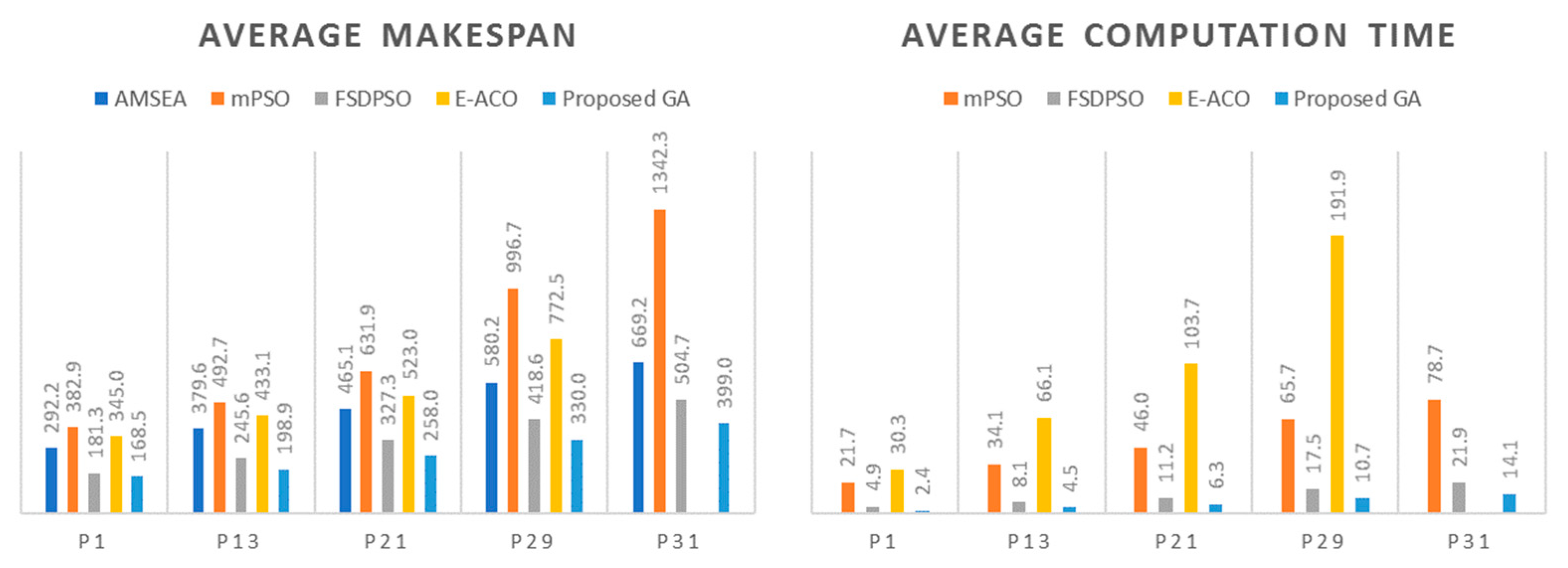
In all the problems, the proposed GA outperformed all other metaheuristics (marked in bold text and gray cells in Table 7) in terms of solution quality and computation time. In Table 7, the improved rate [%] was calculated as $100\left(\mathrm{result}\mathrm{of}\mathrm{FSDPSO}-\mathrm{result}\mathrm{of}\mathrm{Proposed}\mathrm{GA}\right)/\mathrm{result}\mathrm{of}\mathrm{FSDPSO}$. Compared to $C_{max}^{*}$ by FSDPSO, that by the proposed GA was improved by 0.0–27.6% (an average of 14.5%). The proposed GA improved $\overline{C_{max}}$ by 1.9–31.0% (an average of 17.1%) compared to that by FSDPSO. Moreover, the zero $n_{inf}$ for all the problems indicated that all the solutions obtained were feasible. Another notable point is that the computation time of the proposed GA was about 60% of that of FSDPSO. Figure 11 shows the comparison bar charts of $\overline{C_{max}}$ and $\overline{t_{comp}}$ of various methodologies for the five selected problems (P1, P11, P21, P29, and P31). In the figure, regardless of the size of the problem, the proposed GA was superior to other metaheuristics in both solution quality and computation time. FSDPSO had the second-best performance. On the other hand, mPSO had poor solution quality, and E-ACO had weakness in computation time.

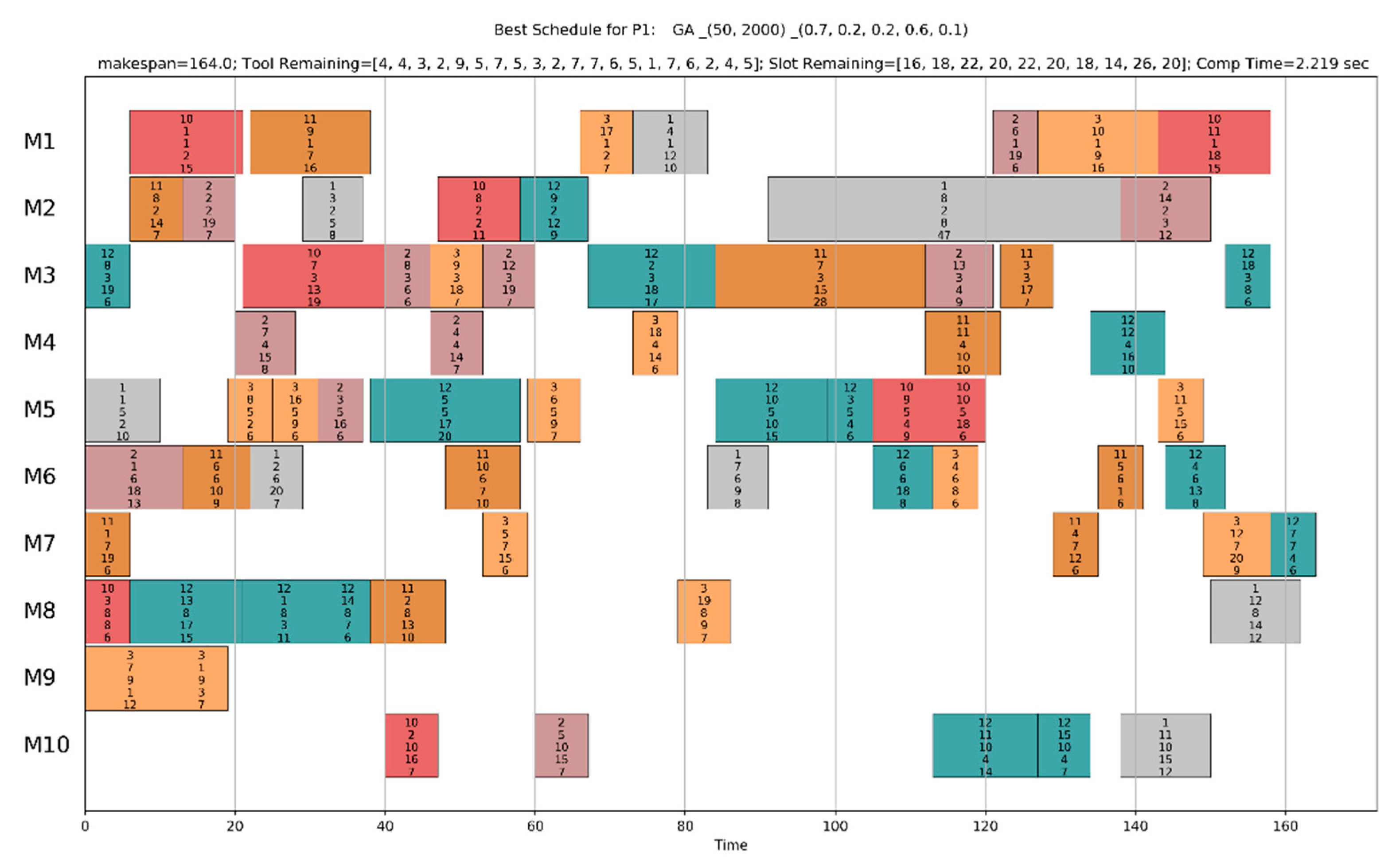
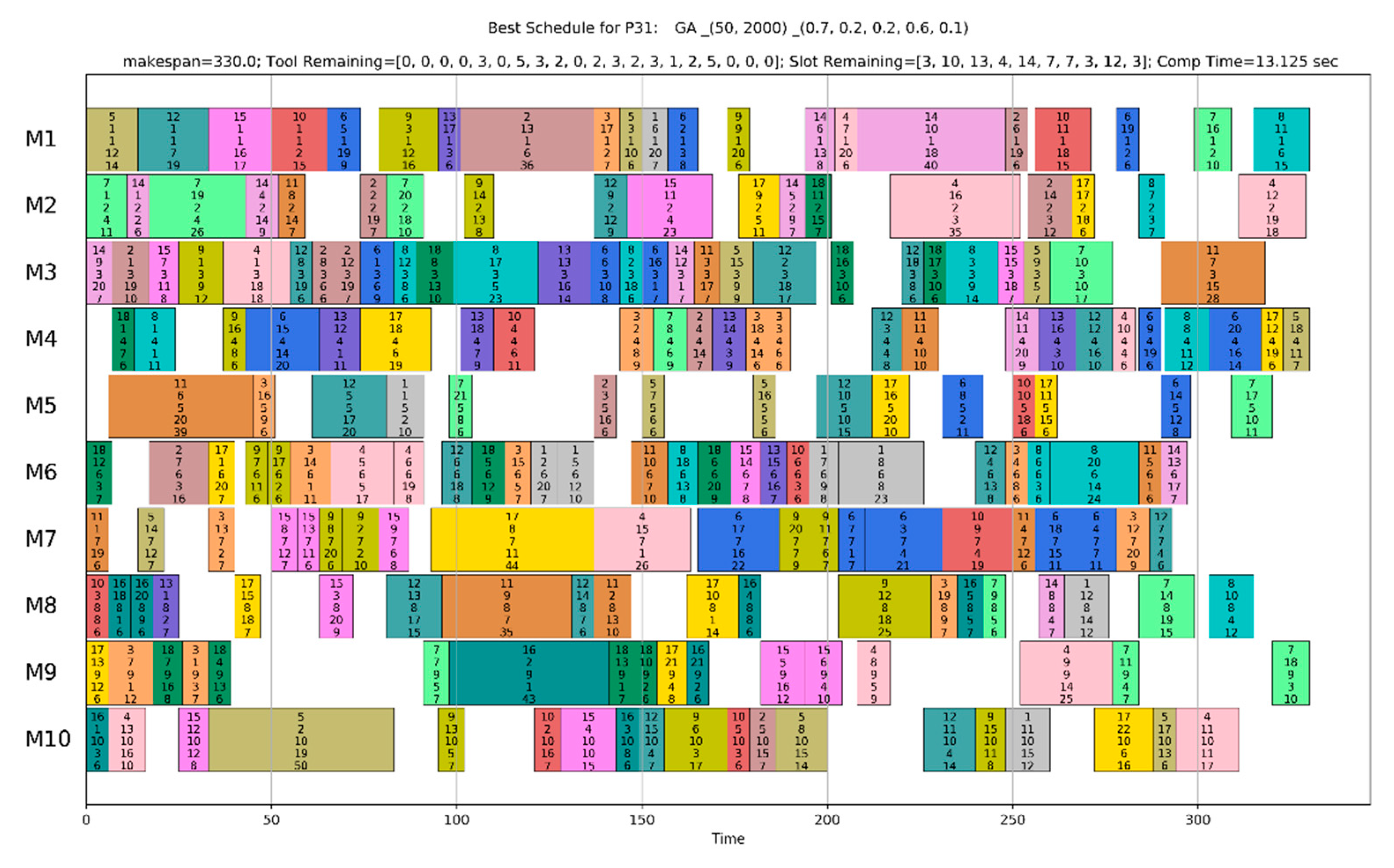
A Gantt chart is a useful tool to easily identify the process plan and the schedule of operations, the final solution of IPPST. Figure 12 and Figure 13 show the Gantt charts of the pseudo-optimal solutions by the proposed GA for P1 and P31, respectively. At the head of the figures, the problem id, the type of metaheuristic, the size of population, the number of generations, the parameter values, the makespan of the solution, the tool remaining at present for each tool type (Tool Remaining), the number of tool slots available at present for each machine (Slot Remaining), and the computation time (Comp Time) are displayed. In both figures, the solutions were feasible because all the values were higher than or equal to zero in Tool Remaining and Slot Remaining. Each colored box represents the schedule (the starting time and the completion time) of each operation, and the internal numbers of each box represent the assigned process plan, that is, the job id, operation id, machine id, tool id, and processing time.

In Figure 12, the schedule for P1, which was a small-sized problem, had many machine idling times (areas without operation boxes, for example, 0–40 sections of M10 in Figure 12). These were generated by the precedence relations between operations and machine availability. To reduce makespan and increase utilization of machines, these idling times should be reduced as much as possible. However, small-sized problems have a limited number of available operations, so reducing the idling times was limited. On the other hand, as shown in Figure 13, large-sized problems such as P31 can be more efficiently scheduled because there are a lot of available operations, so that the number and size of machine idling times are small. Nevertheless, if the makespan is the same, it is recommended that machine idling times be increased to save energy and increase machine and tool lifetime.

7. Discussion

In manufacturing, sustainability has been mainly addressed at strategic levels such as supply chain design, layout design, cleaner product and production mean design, construction, and recycling processes [26]. However, Giret et al. [26] have argued that approaches in operational levels are needed for practical sustainable manufacturing, and they have pointed out that optimization of scheduling can enhance energy efficiency and manageability of oversized capacity. IPPS, which considers process planning and scheduling at the same time, is more practical and useful than scheduling in terms of sustainability because it can eliminate schedule conflicts, reduce process flow time and work-in-process inventory, increase utilization rate, and enhance responsiveness to uncertainties. The limitation of this study was that it did not address the multi-objective problem. Even though makespan is a representative objective variable that potentially contains many factors in IPPS, multi-objective optimization enables detailed control over various sustainable factors such as energy, cost, and greenhouse gas emissions.

Tool flexibility and tool-related constraints are important considerations that determine cost, flexibility, and feasibility, as well as energy consumption. Since the energy efficiency of machine tools is very low [27], efficient operation using scheduling is essential [26]. According to Petrović et al. [8], only four studies [11,28,29,30] in IPPS-related research from 1999 to 2015 considered tool flexibility. Moreover, tool-related constraints such as tool capacity and tool magazine capacity have so far been considered only by Kim et al. [3]. These constraints affect solution quality and resource saving. As shown in the $n_{inf}$ column in Table 7, if the capacities are tight or the size of the problem is large, an infeasible solution is obtained. In addition, even if the solution is feasible, the solution quality is poor because convergence is not sufficient. To pursue sustainable manufacturing at operation levels, additional factors such as sequence-dependent setups, facility maintenance, workpiece loading and unloading, etc., must be considered [31,32]. Since these are generally regarded as constraints, the optimization algorithm must derive a feasible solution under various constraints. Existing algorithms for IPPS do not include constraints other than precedence relations between operations, so performance verification for it is insufficient. On the other hand, the proposed GA efficiently provides a feasible solution even under tool-related constraints, as shown in the experimental results in Table 7.

In the meantime, many optimization methods for IPPS have been proposed. According to Ausaf et al. [33] and Petrović et al. [8], GAs or evolutionary algorithms [3,11,19,34,35,36], ACOs [4,28,37], PSOs [8,11,23,24], and hybrid metaheuristics [8,38] have been most widely used for IPPS optimization. However, they have constructed complex procedures, combined various algorithms, or added specific subprocedures to address the various flexibilities of IPPS and to improve the solution quality of the complex problem. Nevertheless, as shown in the experimental results, the existing metaheuristics do not show remarkable performance. Rather, these approaches, which increase the complexity of the algorithms, result in an increase in computation time without improving the solution quality. On the other hand, even though the GA proposed in this paper follows the conventional simple GA framework, it showed the best performance in terms of both the solution quality and the computation time. This was possible because the proposed integrated chromosome representation could handle the various flexibilities of the IPPS despite the single string structure.

8. Conclusions

The IPPST problem, which is a highly complex combinatorial problem due to various flexibilities, requires complicated representation structures and operating procedures when applying GAs. The main contribution of this study was the implementation of a straightforward simple structured GA for IPPST. To achieve this, we proposed a new chromosome representation. Regarding performance, the proposed GA outperformed the existing metaheuristics for IPPST by over 17% on an average makespan. Decreasing makespan caused an increase in throughput (the amount of production per unit time), which meant that manufacturing capacity increased without additional production facilities. The reduction of makespan also contributes to the profit margin of the company by reducing energy use and manufacturing costs. This not only strengthens the company’s competitiveness and sustainability, but it is also desirable for environmental preservation.

Moreover, the proposed GA could solve even large-sized problems within a short computation time. This means that process planning and scheduling could be solved simultaneously in near-real time by using the proposed GA. The key to smart manufacturing, which has recently been focused on in the manufacturing field, is fast and effective decision making using real-time data. To effectively respond to changes in dynamic manufacturing environments such as emergency orders, cancellation of orders, and machine breakdown, an optimal decision algorithm based on real-time shop floor data is required. The proposed GA is fast and effective, so it can be a countermeasure.

IPPST is constructed under some static assumptions, as mentioned in Section 2. To develop an optimization method that works in a dynamic manufacturing environment, some assumptions must be relaxed. However, such relaxations further increase the complexity of the IPPS and complicate the algorithm for solving the problem. Increasing the complexity of the algorithm degrades efficiency and flexibility, so a more efficient algorithm is needed to solve the problem in real time. Our future work will focus on this topic.

References

- Guerrero, F. Machine loading and part type selection in flexible manufacturing systems. Int. J. Prod. Res. 1999, 37, 1303–1317. [Google Scholar] [CrossRef]
- Kumar, N.; Shanker, K. A genetic algorithm for FMS part type selection and machine loading. Int. J. Prod. Res. 2000, 38, 3861–3887. [Google Scholar] [CrossRef]
- Kim, Y.K.; Kim, J.Y.; Shin, K.S. An asymmetric multileveled symbiotic evolutionary algorithm for integrated FMS scheduling. J. Intell. Manuf. 2007, 18, 631–645. [Google Scholar] [CrossRef]
- Zhang, L.; Wong, T.N. Solving integrated process planning and scheduling problem with constructive meta-heuristics. Inf. Sci. 2016, 340–341, 1–16. [Google Scholar] [CrossRef]
- Nasr, N.; Elsayed, E.A. Job shop scheduling with alternative machines. Int. J. Prod. Res. 1990, 28, 1595–1609. [Google Scholar] [CrossRef]
- Thomalla, C.S. Job shop scheduling with alternative process plans. Int. J. Prod. Econ. 2001, 74, 125–134. [Google Scholar] [CrossRef]
- Stecke, K.E.; Raman, N. FMS planning decisions, operating flexibilities, and system performance. IEEE Trans. Eng. Manag. 1995, 42, 82–90. [Google Scholar] [CrossRef]
- Petrović, M.; Vuković, N.; Mitić, M.; Miljković, Z. Integration of process planning and scheduling using chaotic particle swarm optimization algorithm. Expert Syst. Appl. 2016, 64, 569–588. [Google Scholar] [CrossRef]
- Modi, B.K.; Shanker, K. A formulation and solution methodology for part movement minimization and workload balancing at loading decisions in FMS. Int. J. Prod. Econ. 1994, 34, 73–82. [Google Scholar] [CrossRef]
- Rachamadugu, R.; Stecke, K.E. Classification and review of FMS scheduling procedures. Prod. Plan. Control 1994, 5, 2–20. [Google Scholar] [CrossRef]
- Guo, Y.W.; Li, W.D.; Mileham, A.R.; Owen, G.W. Optimisation of integrated process planning and scheduling using a particle swarm optimisation approach. Int. J. Prod. Res. 2009, 4714, 3775–3796. [Google Scholar] [CrossRef]
- Ho, Y.-C.; Moodie, C.L. Solving cell formation problems in a manufacturing environment with flexible processing and routeing capabilities. Int. J. Prod. Res. 1996, 34, 2901–2923. [Google Scholar] [CrossRef]
- Cheng, R.; Gen, M.; Tsujimura, Y. A tutorial survey of job-shop scheduling problems using genetic algorithms—I. representation. Comput. Ind. Eng. 1996, 30, 983–997. [Google Scholar] [CrossRef]
- Abdelmaguid, T.F. Representations in genetic algorithm for the job shop scheduling problem: A computational study. J. Softw. Eng. Appl. 2010, 3, 1155–1162. [Google Scholar] [CrossRef]
- Giffler, B.; Thompson, G.L. Algorithms for Solving Production-Scheduling Problems. Oper. Res. 1960, 8, 487–503. [Google Scholar] [CrossRef]
- Lian, K.; Zhang, C.; Gao, L.; Li, X. Integrated process planning and scheduling using an imperialist competitive algorithm. Int. J. Prod. Res. 2012, 5015, 4326–4343. [Google Scholar] [CrossRef]
- Liu, M.; Sun, Z.J.; Yan, J.W.; Kang, J.S. An adaptive annealing genetic algorithm for the job-shop planning and scheduling problem. Expert Syst. Appl. 2011, 38, 9248–9255. [Google Scholar] [CrossRef]
- Li, X.; Shao, X.; Gao, L.; Qian, W. An effective hybrid algorithm for integrated process planning and scheduling. Int. J. Prod. Econ. 2010, 126, 289–298. [Google Scholar] [CrossRef]
- Zhang, L.; Wong, T.N. An object-coding genetic algorithm for integrated process planning and scheduling. Eur. J. Oper. Res. 2015, 244, 434–444. [Google Scholar] [CrossRef]
- Shao, X.; Li, X.; Gao, L.; Zhang, C. Integration of process planning and scheduling—A modified genetic algorithm-based approach. Comput. Oper. Res. 2009, 36, 2082–2096. [Google Scholar] [CrossRef] [Green Version]
- Bierwirth, C.; Mattfeld, D.C. Production scheduling and rescheduling with genetic algorithms. Evol. Comput. 1999, 7, 1–17. [Google Scholar] [CrossRef]
- Shi, G. A genetic algorithm applied to a classic job-shop scheduling problem. Int. J. Syst. Sci. 1997, 28, 25–32. [Google Scholar] [CrossRef]
- Miljković, Z.; Petrović, M. Application of modified multi-objective particle swarm optimisation algorithm for flexible process planning problem. Int. J. Comput. Integr. Manuf. 2017, 30, 271–291. [Google Scholar] [CrossRef]
- Dou, J.; Li, J.; Su, C. A discrete particle swarm optimisation for operation sequencing in CAPP. Int. J. Prod. Res. 2018, 56, 3795–3814. [Google Scholar] [CrossRef]
- Zhang, S.; Wong, T.N. Integrated process planning and scheduling: An enhanced ant colony optimization heuristic with parameter tuning. J. Intell. Manuf. 2014, 29, 1–17. [Google Scholar] [CrossRef]
- Giret, A.; Trentesaux, D.; Prabhu, V. Sustainability in manufacturing operations scheduling: A state of the art review. J. Manuf. Syst. 2015, 37, 126–140. [Google Scholar] [CrossRef]
- Hu, S.; Liu, F.; He, Y.; Hu, T. An on-line approach for energy efficiency monitoring of machine tools. J. Clean. Prod. 2012, 27, 133–140. [Google Scholar] [CrossRef]
- Srinivas, P.S.; Raju, V.R.; Rao, C.S.P. Optimization of Process Planning and Scheduling using ACO and PSO Algorithms. Int. J. Emerg. Technol. Adv. Eng. 2012, 2, 343–354. [Google Scholar]
- Li, W.D.; McMahon, C.A. A simulated annealing-based optimization approach for integrated process planning and scheduling. Int. J. Comput. Integr. Manuf. 2007, 20, 80–95. [Google Scholar] [CrossRef] [Green Version]
- Zhang, Y.F.; Saravanan, A.N.; Fuh, J.Y.H. Integration of process planning and scheduling by exploring the flexibility of process planning. Int. J. Prod. Res. 2003, 41, 611–628. [Google Scholar] [CrossRef]
- Zhou, X.; Liu, F.; Cai, W. An energy-consumption model for establishing energy-consumption allowance of a workpiece in a machining system. J. Clean. Prod. 2016, 135, 1580–1590. [Google Scholar] [CrossRef]
- Liao, W.; Wang, T. Promoting Green and Sustainability: A Multi-Objective Optimization Method for the Job-Shop Scheduling Problem. Sustainability 2018, 10, 4205. [Google Scholar] [CrossRef]
- Ausaf, M.F.; Li, X.; Gao, L. Optimization Algorithms for Integrated Process Planning and Scheduling Problem—A Survey. In Proceedings of the Proceeding of the 11th World Congress on Intelligent Control and Automation, Shenyang, China, 29 June–4 July 2014; pp. 5287–5292. [Google Scholar]
- Kim, Y.K.; Park, K.; Ko, J. A symbiotic evolutionary algorithm for the integration of process planning and job shop scheduling. Comput. Oper. Res. 2003, 30, 1151–1171. [Google Scholar] [CrossRef]
- Morad, N.; Zalzala, A. Genetic algorithms in integrated process planning and scheduling. J. Intell. Manuf. 1999, 10, 169–179. [Google Scholar] [CrossRef]
- Li, X.; Gao, L.; Shao, X. An active learning genetic algorithm for integrated process planning and scheduling. Expert Syst. Appl. 2012, 39, 6683–6691. [Google Scholar] [CrossRef]
- Wan, S.Y.; Wong, T.N.; Zhang, S.; Zhang, L. Integrated process planning and scheduling with setup time consideration by ant colony optimization. In Proceedings of the 41st International Conference on Computers and Industrial Engineering, Los Angeles, CA, USA, 23–26 October 2011; pp. 998–1003. [Google Scholar]
- Li, X.; Gao, L. An effective hybrid genetic algorithm and tabu search for flexible job shop scheduling problem. Int. J. Prod. Econ. 2016, 174, 93–110. [Google Scholar] [CrossRef]
Figure 1.
Network representation of an example of IPPST: (a) Network representation example for two jobs; (b) Machine and tool flexibilities of an operation.
Figure 2.
Comparison of operation-based chromosome representations: (a) Typical operation-based representation; (b) Typical permutation of operations-based representation for only active operations; (c) Typical permutation of operations-based representation with additional process route string; (d) Proposed integrated chromosome representation with activation indicator.
Figure 3.
Supporting information for the chromosome representations: (a) Attributes of an operation; (b) Decision rules for the dummy operations in OR relations.
Figure 4.
Pseudocode of the hybrid scheduling procedure for integrated process planning and scheduling (IPPS).
Figure 5.
Pseudocode of the semi-active scheduling procedure for IPPS.
Figure 6.
Overall genetic algorithm (GA) procedure for IPPST.
Figure 7.
Pseudocode of the initial population generation procedure.
Figure 8.
Precedence-preservative crossover (PPX).
Figure 9.
Procedure description of mutations: (a) Location change mutation (LCM); (b) Machine–tool change mutation (MTCM).
Figure 10.
Boxplots depending on the level of parameters: (a) ; (b) .
Figure 11.
Bar graphs of and depending on metaheuristics for the selected problems.
Figure 12.
Gantt chart of the pseudo-optimal solution for P1 by the proposed GA.
Figure 13.
Gantt chart of the pseudo-optimal solution for P31 by the proposed GA.