1. Introduction
Traffic congestion is one of the most significant problems for cities as Colin Buchanan asserted in the 1960s [
1]. Several strategies have been traditionally applied to smooth out congestion, most of them under the umbrella of transportation demand management. In recent years, experts have discussed the implementation of autonomous vehicles (AVs) and their benefits for decongesting cities. For this reason, in some countries, the planning agencies are designing long-term plans, and these agencies need modeling tools that anticipate the impact they may have on transportation networks [
2]. AVs have different levels of automation, and there are multiple definitions for them; NHTSA proposes to use the SAE International’s classification that defines five levels of automation [
3], and the cars are entirely autonomous when they reach level five (L5).
Some experts believe that these cars will widely enter the automotive market during the next decade, others are not so optimistic. Inevitably, AVs will arrive in our cities, and both types of vehicles will share the streets: autonomous and connected vehicles (CAVs) and manual vehicles (MVs) [
4,
5].
Implementation of CAVs will need new technical requirements, which Martínez-Díaz et al. [
6] explain them in detail, for example, a new on-board architecture, sensing system, new communications, cloud requirements, infrastructure needs, and others. This will allow that these new cars could generate positives changes in transportation and urban mobility. For example, the reduction of the generalized transport cost and parking cost of private vehicles, reduction of disutility on travel time, reduction of polluting emissions, improvement in road safety, induced demand, and improvement in road capacity because the distance among vehicles can be less than nowadays [
2,
7].
Several previous researchers have determined the impact of AVs on isolated sections of a highway. The main objective of this research is to analyze the effects of the implementation of CAVs on an urban network. The paper assesses how CAVs will be deployed and will share the infrastructure with MVs by considering three aspects: the potential benefits for the optimal urban structure, the assessment of the direct and indirect impacts of AVs on the efficiency of a network, and the probable effects of the progressive implementation of CAVs. As its focus, this work presents a strategic and macroscopic analysis of CAVs, using a continuous, two-dimensional, total-cost function applied to a circular city. The analysis does not consider other topics such as safety or livability.
We used the continuous approximation method (CA). According to Daganzo [
8], this method was initially proposed by Gordon Newell. Newell formulated a continuous model that obtains the optimal bus schedule of departures from a bus depot, in which the demand function is considered continuous [
9]. If the information concerning the input parameters is not perfect, then the method will be appropriate for solving a problem. The CA method assumes the following conditions: the input data varies slowly over the domain; the total cost is the aggregation of small sub-region costs, and component costs and their constraints depend on the characteristics of these sub-regions [
8]. The CA method has been applied in a wide range of transportation and logistics studies: Clarens and Hurdle [
10], Daganzo [
8], Daganzo and Pilachowski [
11], Medina et al. [
12], Pulido et al. [
13], and others.
In the next section, we explore the impacts of CAVs on mobility. After that, we present the mathematical model and apply it to a case study in a circular city.
2. Theoretical CAV Impacts on Urban Mobility
The classification of AV impacts depends on the type of connection between AVs and the transportation system. AVs should produce positive effects, but some of them will generate non-desirable impacts. These impacts have been explained in various publications [
4,
14,
15], in which [
14] is an extended article of [
4].
2.1. Direct Effects
Firstly, some consequences will directly impact the transportation system; they are positive in general terms, as the literature describes it [
16]. We classify these direct effects in five groups [
4,
14]:
Reduction of generalized travel costs: Efficient driving will create savings in fuel costs and increment the travel speed in all types of vehicles. Furthermore, in a Smart City with V2I communication (vehicle-to-infrastructure), the cars will find a vacant parking spot quickly (on-street or off-street), and the CAVs will directly travel to the parking spot without users at top speed.
Increment of efficiency and flexibility: Driverless vehicles will permit flexibility in operations for transit and taxis, but this could generate a social problem (unemployment). In private AVs, this reduction of cost is not relevant.
Road capacity increment: Previous papers show different results [
7]. Chang and Lai [
17] analyzed the mixed traffic flow in a freeway section; the results show that the increment of road capacity is close to 33%. VanderWerf et al. [
18,
19] studied the impact of autonomous adaptive cruise control (AACC) and cooperative adaptive cruise control (CACC) using traffic simulation. The results show that AACC vehicles will increase the capacity about 7% if the AACC rate is between 40% and 60%; meanwhile, CACC vehicles will increment the capacity to near 102% when all cars are communicated [
19]. Tientrakool et al. [
20] estimated that the road capacity would increase by 43% with AVs and 273% with V2V vehicles. Lioris et al. [
21] stressed that an intersection is the bottleneck of the road capacity. If vehicles with AACC crossed an intersection in a platoon, then the road capacity would be doubled or tripled. Even if cars have CACC technology, the headways will be shorter. In a smart city, CAVs will be more efficient at intersections for V2I technology. On the other hand, other authors disagree and think that AVs would not reduce the congestion because AVs will drive rather cautiously; moreover, it is likely to increase the vehicle-kilometers traveled [
5].
Pollution reduction: Some authors estimate that pollution could decrease [
5,
15] due to these cars will be electric vehicles (optimization of energy consumption) [
6]. On the contrary, other experts predict an increment of this negative externality [
16,
22].
Improvement in road safety: AVs correctly implemented will reduce human errors and negligence in comparison to manual driving [
5,
15], although some estimations have determined that the crash number at roundabouts increases when AVs increase as well [
23].
2.2. Indirect Effects
Secondly, indirect effects will change the demand behavior [
16]. Indirect effects of AVs will cause changes in the system equilibrium between transport supply and demand [
4,
14]. As a result, new requirements for infrastructure will be necessary for the long-term [
24]:
Reduction in the subjective value of travel time savings (VTTS): Ortúzar and Willumsen (2011) define VTTS as “the willingness to pay to reduce travel time by one unit” [
25]. It was first formulated by English economists: Becker (1965), Johnson (1966), Oort (1969), DeSerpa (1971), and Evans (1972) [
25]. Users of AVs will do other tasks instead of driving, reducing the disutility of the travel time [
26].
New users to the vehicle system: AVs will expand the range of users that will use these cars (e.g., minors, the elderly, and disabled people) [
24].
Induced demand: The reduction of the value of time, congestion, and travel times will cause the increment of trip demand in AVs and CAVs. The changes in travel patterns will impact the reduction of transit users [
15], and AV and CAVs could increase. Therefore, this phenomenon will encourage the vicious circle of public transportation [
25].
The increment of vehicle-kilometers traveled (VKT): The increment of the VKT has at least three reasons [
24]. First, splitting of joint trips [
16] in which two or more members of a family that are currently traveling together could travel separately with AVs. Second, AVs will move without passengers (“ghost trips”) [
15,
16]. Moreover, transportation costs will be lower due to a better amortization of a vehicle [
5].
Changes in trip distribution: The improvements due to direct effects, such as the reduction of congestion, costs, and the value of travel time, will cause longer trips. Changes in the place of residence, work, or both will imply changes in the generation and attraction of trips.
Changes in the urban structure and urban activity system: Changes in trip distribution will imply an increment in the city size in the long-term. The urban model will change to a dispersal model (urban sprawl) because new urban areas will be built in places far away from the city center [
24,
27,
28,
29].
There are other impacts that are not less important than the previous ones. First, it could be generated a social opposition to this paradigm shift in mobility due to ethics, legal, environmental, and territorial issues [
6].
3. Mathematical Modeling
Consider a circular city, which has a radius , with circular and radial primary roads in which the demand is continuous. The modeling of a circular city allows obtaining independent results and conclusions of a particular network, but its results apply to many cities that have a radio-centric structure (e.g., Paris, Milan, Moscow, Canberra, Chengdu, Santiago de Chile, and others). In addition, only relevant inputs of the problem are considered to obtain an analytical result that identifies relevant factors and obtains numerical results in reasonable computational times.
The two decision variables of the model are the distance between circulars and radials roads. We consider two types of primary roads (
), and two types of vehicles that use these roads (
), but CAVs travel on dedicated lanes that allow the formation of platoons.
Table A1 describes the continuous spatial variables of the model, and
Table A3 presents the parameters used in the modeling of scenarios with MVs and AVs (
Appendix A).
The formulated model is based on the CA method and has an objective function that represents the total system cost. Therefore, the model solves a system optimum (SO) with a static traffic assignment problem in a continuous space. The CA solves a function of costs, which each point
in polar coordinates (
is the radius and
is the angle in radians) depends on local cost attributes. Total cost function (
in [
$]) results from the integration of the local average cost function of a differential area in polar coordinates (
) over the circular city (
,
). The total cost function (
) has two elements: the total cost of users (
in [
$],
Appendix A) and the agency cost (
in [
$],
Appendix A).
3.1. Demand Modeling
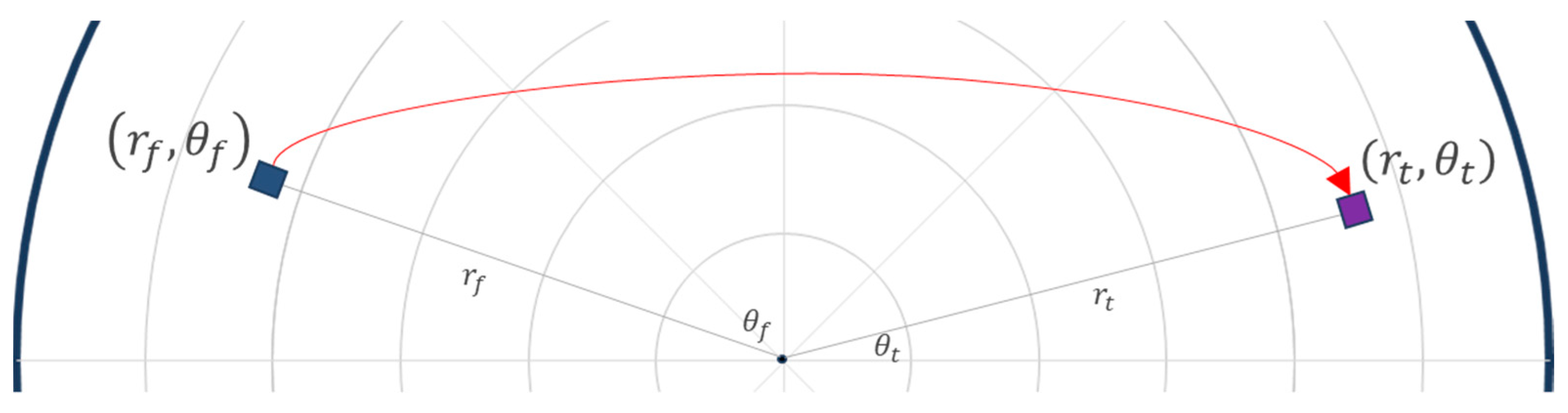
The demand density function
([veh/km
4∙h]) represents the density of car users that begin their trip on the point
and finish it on
[
30] from an infinitesimal area
to other
(
Figure 1). This function allows calculating the generation of trips that access to a primary road, the trip attraction to the destination, and the distribution of trips.
Equation (1) shows the parameter
that is the total number of trips in a circular city with a radius
km where the time of a modeled period is
hours ([h]).
3.2. Trip Assignment
The model assumes that the assignment is a static traffic assignment problem in a continuous space. The incremental assignment is the implemented method, which it is considered a valid approximation for strategic planning. This method divides the distribution matrix at factors (, where is the number of iterations). Thenceforth, the method iteratively assigns to the network each fractioned matrix. In a Smart City with only CAVs, the route assignment should be done by a central agency, which could assign a base matrix using the shortest distance path with the all-or-nothing method and remaining trips using the updated cost function as the incremental method.
Therefore, at Step 0 of this method, the all-or-nothing method is used. For this step, there are three cases [
14]. The cars can take a radial road first and then take a circular road (i.e., a radial–circular trip). In the opposite case, the users take a circular road and, after, a radial road (i.e., a circular–radial trip). Finally, the users take a radial road from the origin to the city center first and, subsequently, they take a radial road to the destination (i.e., a radial–radial trip). In the following steps, the assignment considers the travel time calculated from the accumulated flows. In order to finish the algorithm, the method must sequentially assign all fractions to the network. The results of the assignment are the density functions of demand
Table A2 (
Appendix A).
3.3. Assumptions
The following points summarize the model assumption.
The private transport demand is known, deterministic, and the function varies concerning its position. Furthermore, the car users take the shortest route (minimum distance) to the destination, and they can use circular streets, radial streets, or both of them.
The road capacity is proportional to the number of lanes.
The drivers cannot stop and wait for a vacant parking space and cannot return upstream when they are looking for a parking spot [
31]. The vehicles park on service streets; therefore, they do not cause a reduction of road capacity. The model does not consider the parking capacity.
The model does not include urban freight distribution and public transportation costs.
3.4. Impacts of CAVs on Urban Mobility
In the modeling, the user cost of private trips has three components: accessibility cost to main roads (Equation (A2)), regular trip cost (Equation (A4)), and arriving cost to trip destinations (Equation (A6)). Furthermore, the agency cost contains the infrastructure costs (Equation (A7)). CAVs will impact in different ways at each stage [
4].
Table 1 describes how CAVs will impact on each stage of a trip.
3.5. Mathematical Solution
The mathematical problem is a nonlinear system with constraints from KKT conditions (Equations (A10)). In the CA method, the minimized function is —that is the local cost at each point; the problem has decision variables () and constraints. The optimal analytical formulations are solved through the method of successive approximations.
4. Application to a Case Study
This section has five parts: a description of the case study; parameters; finally, three points with the results of the model.
4.1. Description of a Case Study
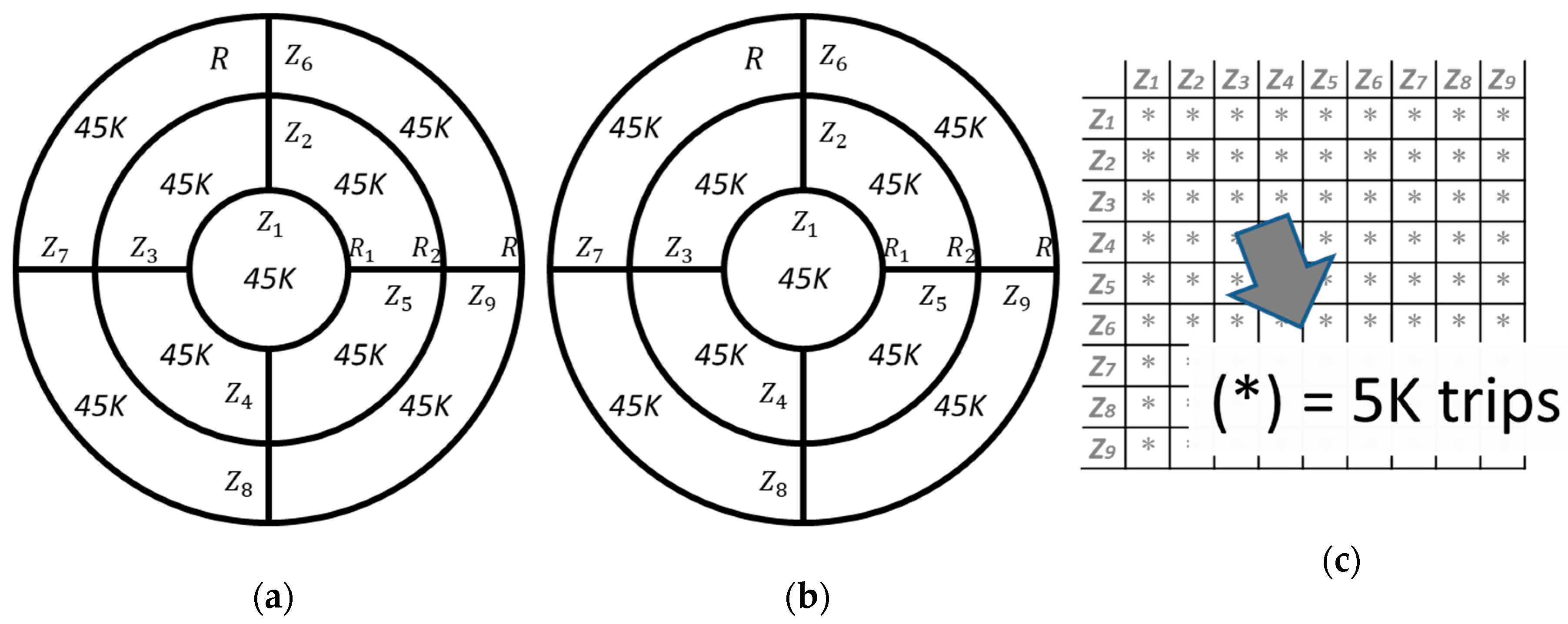
The analyzed case is a circular city with nine zones: a central business district (CBD), four internal zones, and four external zones (
Figure 2a,b). If the city radius is 15 km (
) with a homogeneous trip density, then the CBD radius will be 5 km (
), and the external radius will be about 11.2 km (
). The distribution matrix is symmetric and has 405,000 private trips per hour (
Figure 2c).
The distribution of trip demand (generation, attraction, and trip distribution) allows obtaining the demand density function using the incremental assignment method.
Figure A1 (
Appendix B) shows the density of vehicles that access to main roads, the density of vehicles that travel on main roads, and the density of vehicles that arrive at main roads. Moreover,
Table A4 (
Appendix B) shows the list of parameters for both types of vehicles used by the model.
4.2. Optimal Urban Structure
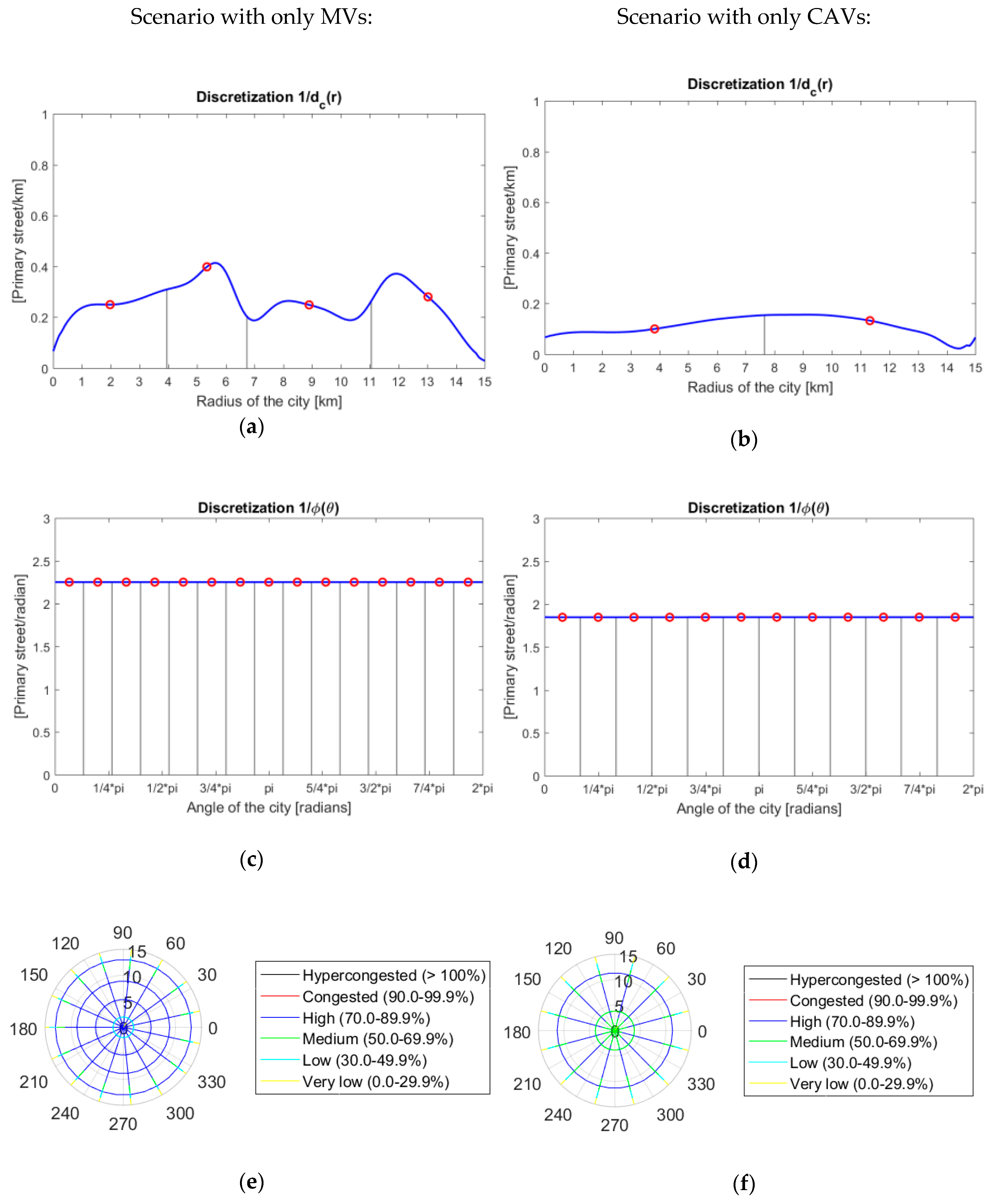
Figure 3 represents the comparison between the results of the optimization with only MVs and CAVs (Level 5 of automation and connected vehicles). The graph (
Figure 3) shows the inverse of the optimal decision variables: distance between circular ((a) and (b)) and radial roads ((c) and (d)). The average of the optimal distance between circular roads is 3.8 km in the base scenario and 7.5 km in the future scenario reducing by half the number of primary roads. In radial roads, the results are similar in both cases. The average optimal distance between radial roads is 2.1 km at a radius of 5 km, 4.1 at 10 km, and 6.2 at 15 km for the current scenario. In the scenario with CAVs, the distance for radial roads is 2.6 km at a radius of 5 km, 5.2 at 10 km, and 7.8 at 15 km. In the discretization, the gray lines represent the border between corridors and the area in this zone is approximately a unit, while the red points represent the location of optimal primary roads.
Finally, the circular graphs (e) and (f) represent the congestion levels on all optimal primary roads of both scenarios. The graphs reveal that the saturation of the future scenario drops, even if there is less road infrastructure supply than in the base scenario.
4.3. Effects on the Urban Network
4.3.1. AV Direct Effects
This section explains some results of direct effects on the urban mobility [
4,
14].
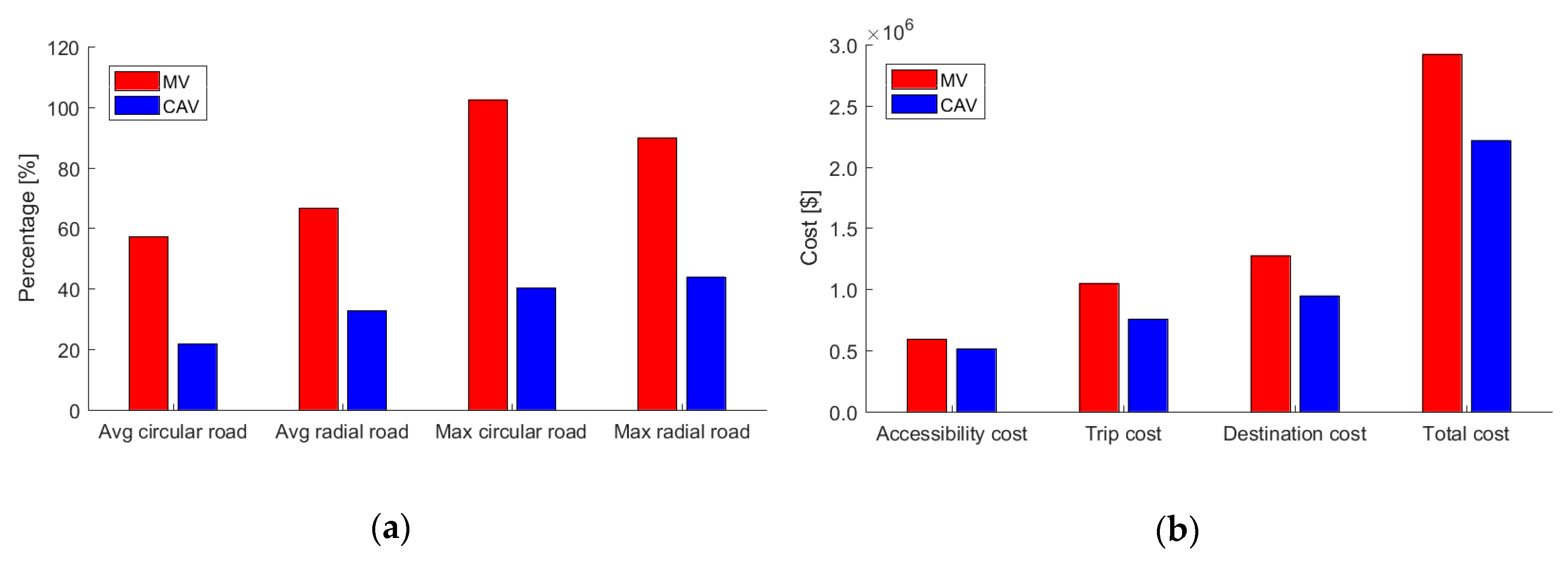
Reduction of road congestion. If the driving of AVs is more efficient than MVs, then the road capacity will rise, and the congestion will drop [
32]. The reduction of the road saturation by CAVs can reach between a third and a half of MV saturation (
Figure 4a).
Reduction of costs. As a result of the previous improvement, the operation cost will also decrease. The cost functions will decrease by about 30%, as shown in
Figure 4b.
4.3.2. AV Indirect Effects
On the other hand, the consequences of AV and CAV indirect effects will offset the savings by direct effects [
4,
14].
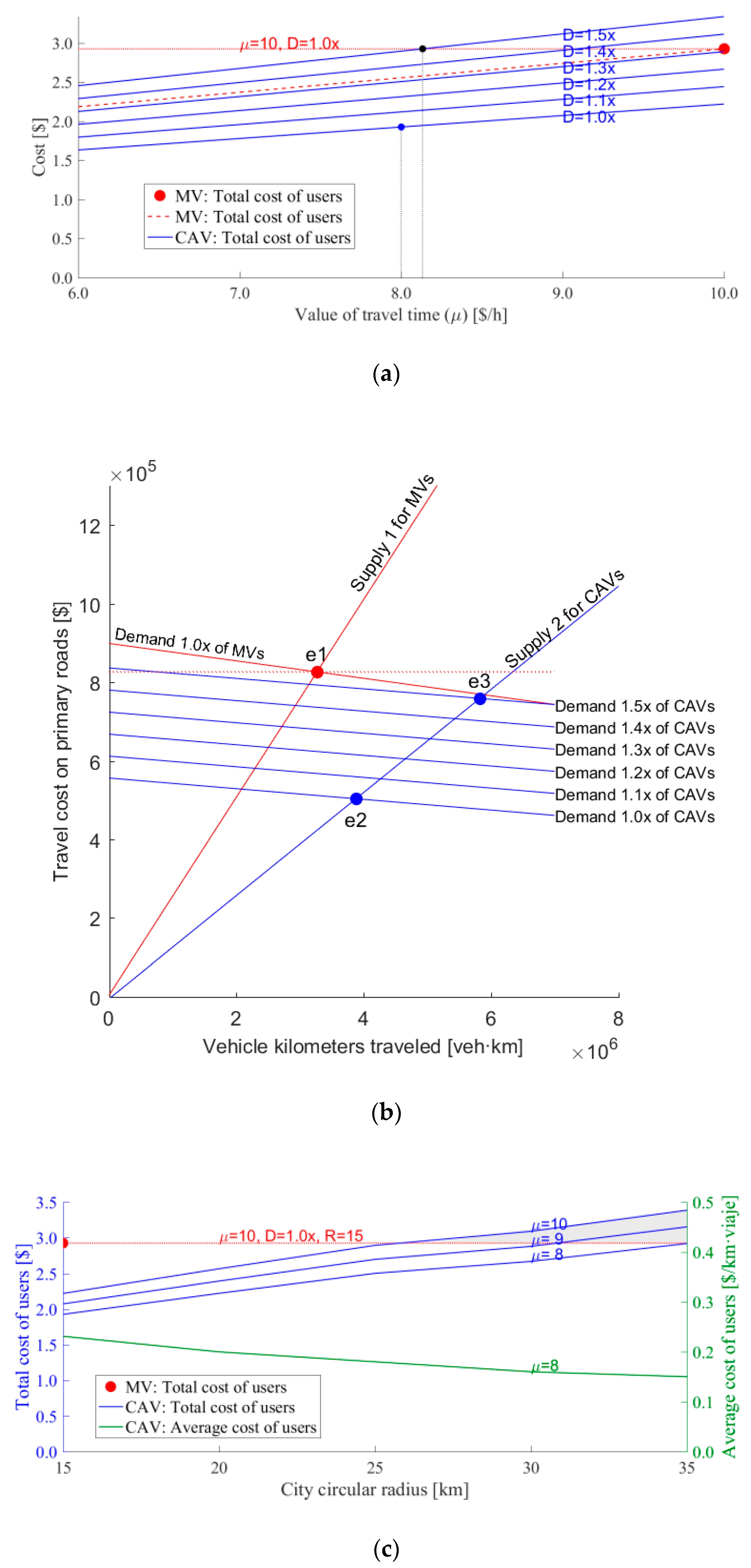
Reduction of the value of travel time.
Figure 5a shows blue lines that represent the reduction of the total cost if the value of travel time decreases and a red point that represents the total cost in the current scenario (only MVs). Kohli and Willumsen [
26] asserted that the value of travel time could decrease by 20% in the scenario with only AVs. Therefore, if
in our model (blue point), then the total cost will decrease by 35%. This is the gap of difference between the red point and the blue point.
Induced demand.
Figure 5b shows the economic model of this system: the price axis represents the travel cost, and the VKT indicator represents the quantity in the horizontal axis. Red lines represent the supply and demand curves for MVs in which the red point (e1) is the current equilibrium. With the operation of only CAVs, the transport supply should increase (blue line). Therefore, the system will have a new equilibrium point (point e2) that will have less congestion than the current scenario, but new users will enter the system. Blue demand lines represent this consequence. If the demand increases 50% (Demand 1.5x), the total cost in the new equilibrium (point e3) will be a little smaller than (or similar to) the current scenario (point e1).
Figure 5a shows that if
, the total costs of the current scenario and the scenario with 1.5x demand are equivalent.
The increment of the VKT. This indicator could increase if AVs started to look for a parking spot only once the user gets out of the car at the destination. The results show an increment of over 5∙10
4 km by CAVs compared to the current scenario [
4,
14], although this result is relative because CAVs will look for a vacant parking space using V2I technology in a Smart City.
Changes in trip distribution and urban structure. If the trips are more extended than nowadays, the city size will increase, and the vicious cycle will be encouraged. Blue lines in
Figure 5c represent the variation of the value of travel time between the city radius and the total cost with only AVs. The graph shows that the total cost will increase if the city grows; hence, this cost could be equivalent to the present scenario (MVs) around a radius of 35 km with
. Therefore, the city size is as considerable as the induced demand. The green curve in
Figure 5c shows that if the urban radius increases, the average user cost per kilometer will slightly decrease. Therefore, if the generalized cost, including the value of time, will be smaller than now, the trips will aim to be longer, and the users will modify the destination. This reduction of costs will cause dispersion along with long-term changes in the activity system and the urban structure. Fortunately, these cars are in the early implementation phases, but urban problems such as spatial segregation or urban sprawl are profound in some cities, and AVs and CAVs could deepen them even more [
4,
14].
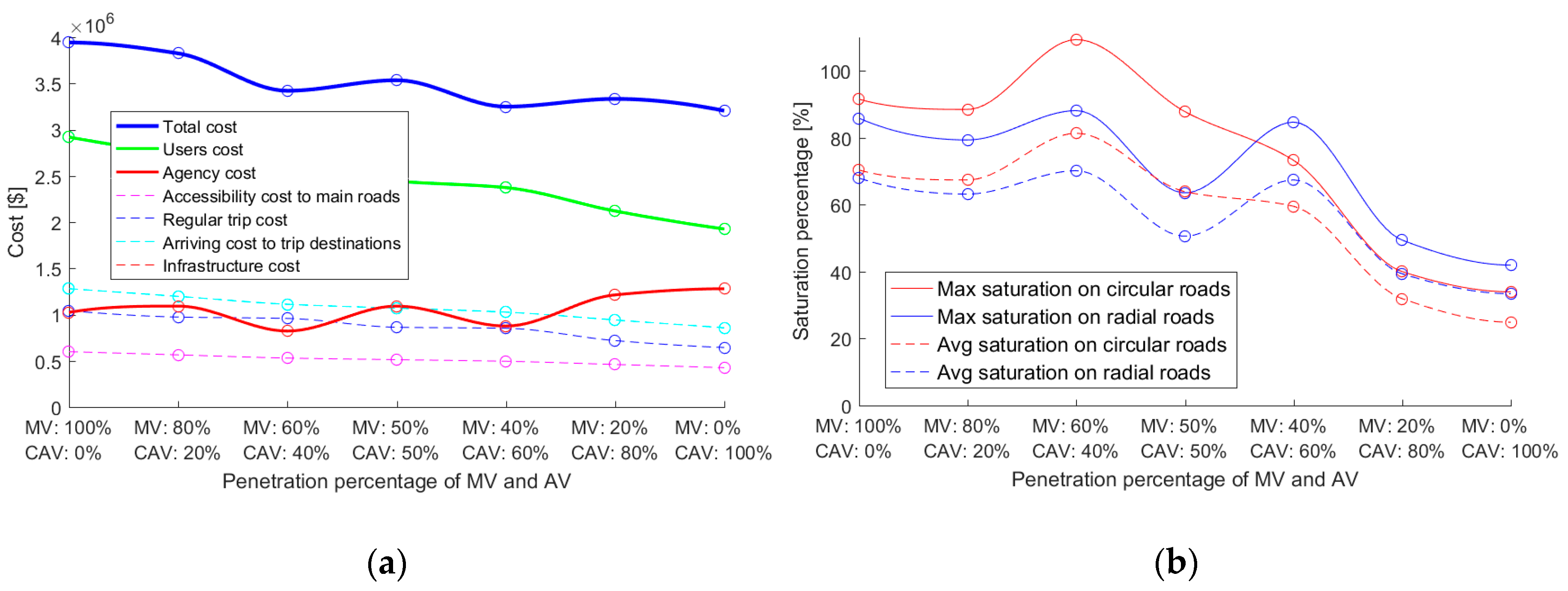
4.4. Progressive Implementation Analysis
We analyze the evolution of the CAV implementation through two factors: the total cost (
Figure 6a) and congestion level (
Figure 6b) by the penetration of CAVs from 0% to 100%. Both charts exhibit that the cost and congestion will decrease with this new technology if the demand is constant over time [
32]. The curve fluctuates when it decreases because the model assigns the infrastructure (number of lanes) progressively according to the type of car, which will generate congestion. In
Figure 6a, the user costs tend to decrease while the agency costs rise when the infrastructure dedicated to CAVs is implemented, reaching almost the convergence when all vehicles are driverless cars. Additionally, the total cost fluctuates, decreasing by the implementation of CAV-dedicated roads. Therefore, agencies have to invest in the mitigating of imbalances between supply and demand.
Figure 6b shows that the gradual implementation could generate scenarios that are worse than the initial stage. In the early years of the implementation, the users’ perception will be averse to incorporating this new automation.
5. Conclusions
Transportation policies should reduce the possible impacts and enhance the potential benefits of AVs. Agencies have to prepare and adapt cities for this change of paradigm in urban mobility. This research seeks to provide some initial ideas on the implementation of new technologies, in which planning agencies should consider them in long-term plans under sustainable development. Consequently, this paper analyzed three topics related to the implementation of CAVs.
First, the direct effects of CAVs will positively impact cities. According to our model, CAVs could influence the optimal structure of a city in two aspects. Firstly, the city will require less road supply. These savings are more significant with circular road supply than in radial roads. This reduction will allow agencies to manage this infrastructure better. Secondly, traffic congestion with CAVs decreases even with less road infrastructure. Despite this, not all of the expected effects are positive.
Second, indirect effects will mitigate the direct effects because the reduction of road capacity is not the only factor of importance. Several significant conclusions can be drawn from the results of this work. Firstly, the value of travel time is another crucial factor. On the one hand, it can reduce a third of the total cost; on the other hand, it might cause other significant externalities explained in the following points. Secondly, the induced demand is another element that might limit the benefits obtained through CAVs. Thirdly, the increment of vehicle-kilometers traveled is a difficult factor to measure, but the consequences can be substantial over the city. Finally, the dispersion of cities is a factor that has not received as much attention, and they have been less researched than others impacts of AVs. Thus, urban growth could be more significant than other factors, such as induced demand. All factors as a whole will tend to encourage the vicious cycle of public transportation and to promote unsustainable cities in the long-term.
Third, the analysis done on the progressive implementation of CAVs shows that the operation of these cars will be a complicated process, as reaching the optimal equilibrium requires additional resources for reducing possible scenarios as bad as the current scheme.
The three aspects previously analyzed expose the advantages and limitations of the implementation of CAVs from the point of view of travel costs. Therefore, a city with only CAVs will not be sustainable; urban sustainability will only be kept using complementary modes such as public and shared transportation. Moreover, these changes will boost the operation of new technologies such as shared autonomous vehicles (SAV), mobility as a service (MaaS), personal mobility devices (electric scooters, Segways, hoverboards, unicycles), and others.
In future works, the model will permit the proposal of different solutions in a city with heterogeneous demand spatially. Moreover, the influence of changes in user behavior will be analyzed in each stage of the trip, considering aspects such as modal choice, trip distribution, and assignment. Finally, in future analysis, we will also consider extending the study to the case of a real city.
Author Contributions
Conceptualization, M.M.-T. and F.R.; Formal analysis, M.M.-T. and F.R.; Methodology, M.M.-T.; Writing—original draft, M.M.-T.; Writing—review & editing, M.M.-T. and F.R.
Funding
This study had support from the Project 061312MT of the Departamento de Investigaciones Científicas y Tecnológicas (DICYT) of the Vicerrectoría de Investigación, Desarrollo e Innovación of the Universidad de Santiago de Chile (USACH). It also had support from Abertis endowed Chair at BarcelonaTech.
Acknowledgments
Marcos Medina-Tapia and Francesc Robusté are members of BIT-Barcelona Innovative Transportation research group at BarcelonaTech. Marcos Medina-Tapia was also supported by CONICYT PFCHA/BCH 72160291 scholarship.
Conflicts of Interest
The authors declare no conflict of interest. The funders had no role in the design of the study; in the collection, analyses, or interpretation of data; in the writing of the manuscript, or in the decision to publish the results. The contents of this paper reflect the views of the authors, who are responsible for the facts and accuracy of the data presented herein.
Appendix A
This section describes the mathematical formulation. The total cost function (
) has two elements: the total cost of users (
in [
$]) and the agency cost (
in [
$]). The model uses continuous spatial variables (
Table A1); secondly,
Table A2 describes the demand density functions obtained from the assignment method. Finally,
Table A3 presents the list of parameters used in the modeling of a circular city.
Table A1.
Variables used in the modeling of a circular city.
Table A1.
Variables used in the modeling of a circular city.
| Variables |
|---|
| distance function between circular roads of type at the radius km [km/road]; and |
| angle function between radial roads of type at a city point with angle [radian/road], which is the distance function between radial roads at a city point [km/road]. |
Table A2.
Demand density functions obtained from the assignment method.
Table A2.
Demand density functions obtained from the assignment method.
| Demand Functions |
|---|
| vehicles density of type that access from the origin to a circular () or radial () primary road [veh/km2∙h]; |
| vehicle flow density of type that travel on a circular () or radial () primary road considering the direction [veh/km∙h]; and |
| vehicles density of type that arrive from a circular () or radial () primary road to the destination [veh/km2∙h]. |
Table A3.
Nomenclature of parameters used in the modeling of a circular city.
Table A3.
Nomenclature of parameters used in the modeling of a circular city.
| Other Parameters |
|---|
| duration of period [h]; |
| value of travel time of users in vehicle [$/h]; |
| car speed of type to access main roads of the city [km/h]; |
| free-flow car speed of type on a primary road of type [km/h]; |
| cruising speed of a car looking for a parking spot [km/h]; |
| average walking speed for accessing to the destination point from parking site [km/h]; |
| average time for accessing the primary road of a car [h]; |
| average time for accessing the local roads from a road of a car [h]; |
| and | parameters of BPR volume-delay function [dimensionless]; |
| capacity road per lane of type [veh/lane∙h]; |
| number of lanes at a road [lane]; |
| average time spent by a vehicle of type when crosses a crossroad on a road of type [h/veh]; |
| average density of vacant parking space [parking/km]; |
| distance before arriving at the destination where the drivers begin to look for a parking spot [km]; |
| car cost of type per distance unit [$/km∙veh]; |
| parking fee [$/h∙veh]; |
| maintenance fixed cost by road infrastructure for a road and a car [$/km]; and |
| maintenance variable cost by road infrastructure for a road and a car [$/km∙h]. |
Appendix A.1. Users Costs
The total user cost function ( in []) contains three elements: accessibility cost to a primary road (), cost spent in a regular car trip (), and arriving cost at the destination ().
Appendix A.1.1. Accessibility Cost to Main Roads
The average access cost (Equation (A1) in
) for accessing to a circular (
) or a radial road (
) has two components. First, cars travel a quarter of the distance between the origin and the closest primary road. The average travel cost is the multiplication of this distance and the generalized cost
(
in
). Second, the users incur a cost for accessing the primary road (
where
in
).
The local accessibility cost function has two components: the demand density in rush hour (
) and the average access cost per vehicle (
). This cost is the integration of a local cost over the city area for all types of roads
and vehicles
(Equation (A2)).
Appendix A.1.2. Regular Trip Cost
In regular trips, the generalized travel cost function has three elements (Equation (A3) in
). The first component is a Bureau of Public Roads (BPR) function that represents the congestion effects. The free-flow travel cost per kilometer is the inverse of free-flow speed multiplied by the value of travel time (
). The congestion level depends on the traffic flow (
and
) and the capacity of the road type
(
) where the vehicles can travel in two directions:
on circular roads, and
on radial roads. Secondly, the unitary cost of a regulated crossroad by traffic lights is the ratio between the cost spent by crossing the road (
) and the distance between roads (
or
). Finally, the last component is the operational cost (
).
Similar to the previous case, the total trip cost (
in
) is the integration of the local cost function. The elements of the local cost function are the demand density in rush hour and the local generalized travel cost in each type of road
(Equation (A4)).
Appendix A.1.3. Arriving Cost to Trip Destinations
After that a user has parked his car, he has to pay for the parking fee and has to walk to the final destination. The average destination cost has five elements. Firstly, the users incur a cost for accessing local roads (
where
in
). Secondly, the driving cost on local streets before the users start to look for a vacant parking spot. This sub-cost is composed of the average distance (e.g.,
) and the generalized cost (
). Thirdly, the cost incurred by users, which are looking for a parking space, is the multiplication of the average distance between vacant spots (
) and the generalized cost (
). Fourthly, the user walking cost, which is the distance between the user parked and the destination, is the multiplication of the expected walking distance and the generalized cost (
). According to Arnott and Rowse [
31], the expected walking distance after parking the vehicle has two cases. If a driver finds a vacant space before his destination (
) then this driver will walk
km. In another case, the driver will walk
km to the destination. Finally, the cost includes the car parking fee (
). Equation (A5) shows the average local destination cost (
) for each road type.
The total arriving cost (
in
, Equation (A6)) is the integration of the local cost composed of the demand function in rush period (
), and the expected walking cost and parking fee (
).
Appendix A.2. Agency Costs
In the agency cost (
in [
], Equation (A7)), the local cost function (
) is the multiplication of the cost per linear kilometer and the road density (
or
). The unitary cost contains two parts: a fixed and a variable element.
Appendix A.3. Constraints
The model also considers that the congestion should not overtake 90 percent of capacity for both roads (Equations (A8) and (A9)).
Appendix A.4. Numerical Solution
The nonlinear system has
decision variables (
) and
constraints. The set of Equation (A10) shows the KKT conditions, in which we obtain the first condition for each one of the decision variables (A10.1) when they are not negative (A10.5). The second condition contains the constraints
(A10.2). The third condition set is the complementary slackness (A10.3); if the inequality constraint is active, its slack is zero, and its multiplier (
) takes any non-negative value (A10.4). In Equation (A10), the expression contains an equation system with inequalities. This system of equations allows obtaining the optimal solution through the method of successive approximations.
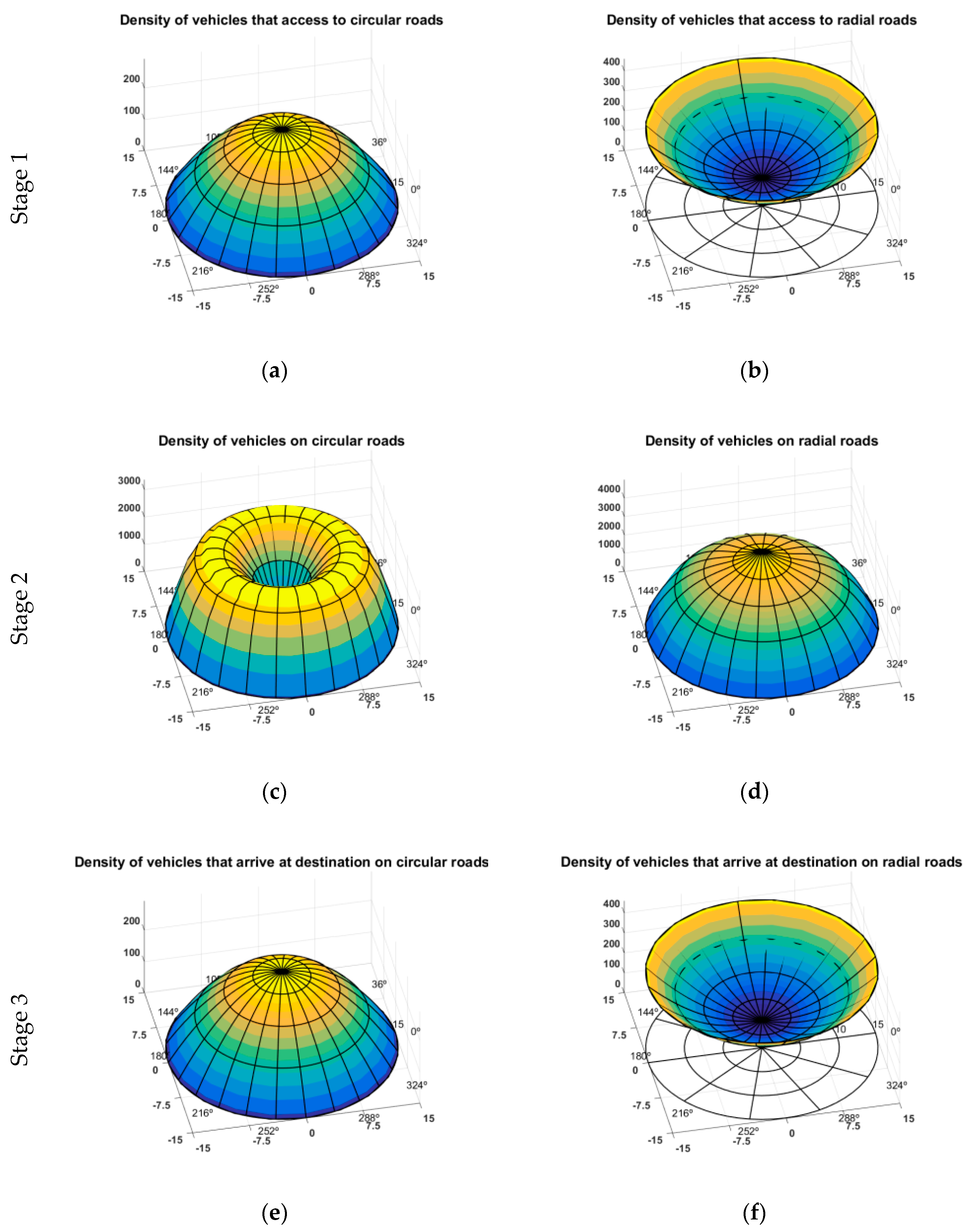
Figure A1.
Traffic density assignment in rush period (K is a thousand trips): (a) Density of vehicles that access to circular roads. (b) Density of vehicles that access to radial roads. (c) Density of vehicles on circular roads. (d) Density of vehicles on radial roads. (e) Density of vehicles that arrive at the destination on circular roads. (f) Density of vehicles that arrive at the destination on radial roads.
Appendix B
This section presents the inputs used in the modeling: demand and other parameters.
Appendix B.1. Demand
Figure A1 shows the homogeneous demand density with only MVs in each car trip stage using the incremental assignment method. In Stage 1, the density of generated and attracted trips in an infinitesimal area (
) is concentrated on the central zone for trips that access circular primary roads (
Figure A1a) and on the periphery for radial roads (
Figure A1b). In Stage 2, the regular trip density at each city point (
) is concentrated in an internal zone for circular roads (
Figure A1c). On the other hand, radial trips are concentrated around the city center (
Figure A1d). In Stage 3, the density represents attracted trips around a point (
) concerning trips that arrive from circular (
Figure A1e) and radial roads (
Figure A1f). Similar to Stage 1, the majority of attracted trips from circular roads are around the central area, whereas the most density of radial trips is in external zones [
14].
Appendix B.2. Parameters
Table A4 shows the parameter list of both types of vehicles used by the model. Our model considers that the value of travel time will be equal for each type of car users [
14]. The average value is based on Litman’s report [
33].
In arterial roads, the capacity of urban roads depends on the intersection capacity [
21]. AACC allows the formation of platoons, although the headway could improve if the cars have CACC. In the current scheme with only MVs, the capacity of streets is 1,272 per lane (
) [
21]. In a future scenario with AVs, the road capacity will be 3,960 (
); it is three times bigger than the present scenario as stated in Lioris et al. [
21]. For freeways, the investigations show that MVs can reach the capacity of 2,099 [veh/lane∙h]. On the other hand, AACC vehicles will increase the road capacity about 7% if the ratio of AACC is between 40% and 60% [
18,
19], while the CACC vehicles increase the capacity about 102% when all vehicles are communicated (4,259 [veh/lane∙h]). Therefore, in the modeling, the case of AVs includes the connected and automated vehicles (CAVs). In the modeling, arterial roads have six lanes and freeways have eight lanes. The lanes will distribute between MVs and AVs because of the number of lanes depends on the type of road and the penetration of AVs. In AV lanes, these cars will form platoons.
Table A4.
Parameters used in each scenario.
Table A4.
Parameters used in each scenario.
| Parameters | Case of MVs | Case of CAVs |
|---|
| (h) | 1.5 | 1.5 |
| ($/h) | 10 | 8 |
| (km/h) | 25 | 30 |
| (km/h) | : 45; : 95 | : 50; : 100 |
| (km/h) | 10 | 30 |
| (km/h) | 3 | 3 |
| (h) | : 45/3600; : 5/60 | : 45/3600; : 5/60 |
| | 2 | 2 |
| | 3 | 3 |
| (veh/lane∙h) | : 1,272; : 2,099 | : 3,960; : 4,259 |
| (lane) | : [0…6]; : [0…8] | : [0…6]; : [0…8] |
| (h/veh) | : 0.0125; : 0 | : 0.0125∙70%; : 0 |
| (parking/km) | 5 | 5 |
| (km) | 0.2 | 0.0 |
| ($/km∙veh) | 0.1 | 0.1∙50% |
| ($/h∙veh) | 1 | 1 |
| ($/km) | : 5.680∙106; : 10.85∙106 | |
| ($/km∙h) | | |
We assume that the mileage in MVs is 10 km/L and the fuel price is 1
$/L. Moreover, we assume AVs will save 50% in comparison to a conventional car [
34]. Moreover, we assume that the parking fee is
[
$/veh∙h]. Furthermore, the fixed unit cost value is based on the paved cost per linear meter built, and the lifetime of the road project divides it. The cost per kilometer is based on technical reports of Arkansas’s Department of Transportation [
35]. The variable unitary cost can be considered as the 1% of fixed cost (
). Finally, we assume that the infrastructure cost for AVs is 25% more expensive than the infrastructure for MVs.
References
- Buchanan, C. Traffic in Towns: A Study of the Long Term Problems of Traffic in Urban Areas, 1st ed.; Her Majesty’s Stationery Office: London, UK, 1963; ISBN 0115503161. [Google Scholar]
- Childress, S.; Nichols, B.; Charlton, B.; Coe, S. Using an Activity-Based Model to Explore the Potential Impacts of Automated Vehicles. Transp. Res. Rec. J. Transp. Res. Board 2015, 2493, 99–106. [Google Scholar] [CrossRef]
- National Highway Traffic Safety Administration (NHTSA). Federal Automated Vehicles Policy; US Department of Transportation: Washington, DC, USA, 2016.
- Medina-Tapia, M.; Robusté, F. Exploring paradigm shift impacts in urban mobility: Autonomous Vehicles and Smart Cities. Transp. Res. Procedia 2018, 33, 203–210. [Google Scholar] [CrossRef]
- Martínez-Díaz, M.; Soriguera, F.; Pérez, I. Technology: A Necessary but Not Sufficient Condition for Future Personal Mobility. Sustainability 2018, 10, 4141. [Google Scholar] [CrossRef]
- Martínez-Díaz, M.; Soriguera, F.; Pérez, I. Autonomous driving: A bird’s eye view. IET Intell. Transp. Syst. 2018, 1–17. [Google Scholar] [CrossRef]
- Kockelman, K. An Assessment of Autonomous Vehicles: Traffic Impacts and Infrastructure Needs; Center for Transportation Research, University of Texas: Austin, TA, USA, 2017. [Google Scholar]
- Daganzo, C.F. Logistics Systems Analysis, 4th ed.; Springer: Berlin, Germnay, 2005; ISBN 3540275169. [Google Scholar]
- Newell, G.F. Dispatching Policies for a Transportation Route. Transp. Sci. 1971, 5, 91–105. [Google Scholar] [CrossRef]
- Clarens, G.C.; Hurdle, V.F. An Operating Strategy for a Commuter Bus System. Transp. Sci. 1975, 9, 1–20. [Google Scholar] [CrossRef]
- Daganzo, C.F.; Pilachowski, J. Reducing bunching with bus-to-bus cooperation. Transp. Res. Part B Methodol. 2011, 45, 267–277. [Google Scholar] [CrossRef]
- Medina-Tapia, M.; Giesen, R.; Muñoz, J.C. Model for the Optimal Location of Bus Stops and its Application to a Public Transport Corridor in Santiago, Chile. Transp. Res. Rec. J. Transp. Res. Board 2013, 2352, 84–93. [Google Scholar] [CrossRef]
- Pulido, R.; Muñoz, J.C.; Gazmuri, P. A Continuous Approximation Model for Locating Warehouses and Designing Physical and Timely Distribution Strategies for Home Delivery. EURO J. Transp. Logist. 2015, 4, 399–419. [Google Scholar] [CrossRef]
- Medina-Tapia, M.; Robusté, F. Exploring paradigm shift impacts in urban mobility: Autonomous Vehicles and Smart Cities. In Proceedings of the XIII Conference on Transport Engineering (CIT 2018), Gijón, Spain, 6–8 June 2018. [Google Scholar]
- Pakusch, C.; Stevens, G.; Boden, A.; Bossauer, P. Unintended Effects of Autonomous Driving: A Study on Mobility Preferences in the Future. Sustainability 2018, 10, 2404. [Google Scholar] [CrossRef]
- Bahamonde-Birke, F.J.; Kickhöfer, B.; Heinrichs, D.; Kuhnimhof, T. A Systemic View on Autonomous Vehicles. Policy Aspects for a Sustainable Transportation Planning. disP Plan. Rev. 2018, 54, 12–25. [Google Scholar] [CrossRef]
- Chang, T.H.; Lai, I.S. Analysis of characteristics of mixed traffic flow of autopilot vehicles and manual vehicles. Transp. Res. Part C Emerg. Technol. 1997, 5, 333–348. [Google Scholar] [CrossRef]
- VanderWerf, J.; Shladover, S.; Kourjanskaia, N.; Miller, M.; Krishnan, H. Modeling Effects of Driver Control Assistance Systems on Traffic. Transp. Res. Rec. J. Transp. Res. Board 2001, 1748, 167–174. [Google Scholar] [CrossRef]
- VanderWerf, J.; Shladover, S.; Miller, M.; Kourjanskaia, N. Effects of Adaptive Cruise Control Systems on Highway Traffic Flow Capacity. Transp. Res. Rec. J. Transp. Res. Board 2002, 1800, 78–84. [Google Scholar] [CrossRef]
- Tientrakool, P.; Ho, Y.-C.; Maxemchuk, N.F. Highway Capacity Benefits from Using Vehicle-to-Vehicle Communication and Sensors for Collision Avoidance. In Proceedings of the 2011 IEEE Vehicular Technology Conference (VTC Fall), San Francisco, CA, USA, 5–8 September 2011; pp. 1–5. [Google Scholar]
- Lioris, J.; Pedarsani, R.; Tascikaraoglu, F.Y.; Varaiya, P. Platoons of connected vehicles can double throughput in urban roads. Transp. Res. Part C Emerg. Technol. 2017, 77, 292–305. [Google Scholar] [CrossRef] [Green Version]
- Wadud, Z.; MacKenzie, D.; Leiby, P. Help or hindrance? The travel, energy and carbon impacts of highly automated vehicles. Transp. Res. Part A Policy Pract. 2016, 86, 1–18. [Google Scholar] [CrossRef] [Green Version]
- Deluka Tibljaš, A.; Giuffrè, T.; Surdonja, S.; Trubia, S. Introduction of Autonomous Vehicles: Roundabouts Design and Safety Performance Evaluation. Sustainability 2018, 10, 1060. [Google Scholar] [CrossRef]
- Smith, B.W. Managing Autonomous Transportation Demand. Santa Clara Law Rev. 2012, 52, 1401–1422. [Google Scholar]
- Ortúzar, J. de D.; Willumsen, L.G. Modelling Transport, 4th ed.; John Wiley: Chichester, UK, 2011; ISBN 9780470760390. [Google Scholar]
- Kohli, S.; Willumsen, L.G. Traffic forecasting and automated vehicles. In Proceedings of the 44th European Transport Conference, Barcelona, Spain, 5–7 October 2016. [Google Scholar]
- Meyer, J.; Becker, H.; Bösch, P.M.; Axhausen, K.W. Autonomous vehicles: The next jump in accessibilities? Res. Transp. Econ. 2017, 62, 80–91. [Google Scholar] [CrossRef] [Green Version]
- Zakharenko, R. Self-driving cars will change cities. Reg. Sci. Urban Econ. 2016, 61, 26–37. [Google Scholar] [CrossRef]
- Zhang, W.; Guhathakurta, S.; Fang, J.; Zhang, G. Exploring the impact of shared autonomous vehicles on urban parking demand: An agent-based simulation approach. Sustain. Cities Soc. 2015, 19, 34–45. [Google Scholar] [CrossRef]
- Vaughan, R. Optimum Polar Networks for an Urban Bus System with a Many-to-Many Travel Demand. Transp. Res. Part B Methodol. 1986, 20, 215–224. [Google Scholar] [CrossRef]
- Arnott, R.; Rowse, J. Modeling Parking. J. Urban Econ. 1999, 45, 97–124. [Google Scholar] [CrossRef]
- Medina-Tapia, M.; Robusté, F. Impact assessment of autonomous vehicle implementation on urban road networks. In Proceedings of the Pan-American Conference of Traffic, Transportation Engineering and Logistics (PANAM), Medellin, Colombia, 26–28 September 2018. [Google Scholar]
- Litman, T. Transportation Cost and Benefit Analysis Techniques, Estimates and Implications; Victoria Transport Policy Institute: Victoria, Australia, 2016. [Google Scholar]
- Litman, T. Autonomous Vehicle Implementation Predictions: Implications for Transport Planning; Victoria Transport Policy Institute: Victoria, Australia, 2018. [Google Scholar]
- Arkansas Department of Transportation (ARDOT). Estimated Costs Per Mile. Available online: https://www.arkansashighways.com/ (accessed on 1 June 2018).
© 2019 by the authors. Licensee MDPI, Basel, Switzerland. This article is an open access article distributed under the terms and conditions of the Creative Commons Attribution (CC BY) license (http://creativecommons.org/licenses/by/4.0/).


